DDPG-Based Adaptive Sliding Mode Control with Extended State Observer for Multibody Robot Systems

Abstract

This research introduces a robust control design for multibody robot systems, incorporating sliding mode control (SMC) for robustness against uncertainties and disturbances. SMC achieves this through directing system states toward a predefined sliding surface for finite-time stability. However, the challenge arises in selecting controller parameters, specifically the switching gain, as it depends on the upper bounds of perturbations, including nonlinearities, uncertainties, and disturbances, impacting the system. Consequently, gain selection becomes challenging when system dynamics are unknown. To address this issue, an extended state observer (ESO) is integrated with SMC, resulting in SMCESO, which treats system dynamics and disturbances as perturbations and estimates them to compensate for their effects on the system response, ensuring robust performance. To further enhance system performance, deep deterministic policy gradient (DDPG) is employed to fine-tune SMCESO, utilizing both actual and estimated states as input states for the DDPG agent and reward selection. This training process enhances both tracking and estimation performance. Furthermore, the proposed method is compared with the optimal-PID, SMC, and $H_{\infty }$ in the presence of external disturbances and parameter variation. MATLAB/Simulink simulations confirm that overall, the SMCESO provides robust performance, especially with parameter variations, where other controllers struggle to converge the tracking error to zero.

1. Introduction

The expanding capabilities of multibody robot systems in autonomous operation and their versatility in performing a wide range of tasks have gathered significant attention from both researchers and industries, emphasizing the persistent need for precision and reliability in their operations. As a result, multibody robot systems require robust control algorithms. However, controlling multibody robot dynamics can be a challenging task, especially when the robot dynamics are unknown. In this effort, different robust control algorithms have been proposed in which sliding mode control (SMC) has been of great interest due to outstanding robustness against parametric uncertainties and external disturbances [1,2]. Subsequent developments resulted in different types of SMC, including integral SMC (ISMC) [3], super twisting SMC (STSMC) [4], terminal SMC (TSMC) [5], SMC with a nonlinear disturbance observer known as sliding perturbation observer (SMCSPO) [6], and SMC with extended state observer (SMCESO) [7].

This research is conducted for the robust control of multibody industrial robot systems with aims of enhancing the trajectory tracking results. Therefore, we consider the nonlinear control SMC with ESO (SMCESO) for the robot control. ESO considers the system dynamics and external disturbances as perturbations to the system. Therefore, with ESO, the system is only affected by the perturbation estimation error because of the compensation provided by the ESO. Another advantage of the ESO is that it requires no system dynamics information and only uses partial state feedback (position) for estimating the states and the perturbation. Subsequently, the robustness of SMCESO now depends on the quality of estimation of the ESO, which is dependent on the selection of control parameters. However, tuning the parameters manually becomes a challenging task. Therefore, optimal parameter selection can be achieved through adapting the parameters for different sliding conditions.

Various methods for adaptive SMC have been explored, including model-free adaptation, intelligent adaptation, and observer-based adaptation. A. J. Humaidi et al. introduced particle swarm optimization-based adaptive STSMC [8]. The adaptation is carried out based on the Lyapunov theory to guarantee global stability. Y. Wang and H. Wang introduced model-free adaptive SMC, initially estimating unknown dynamics through the time delay estimation method [9,10]. Nevertheless, this approach exhibited undesirable chattering in the control input during experiments, which is deemed unacceptable in the present research. On the other hand, R-D. Xi et al. presented adaptive SMC with a disturbance observer for robust robot manipulator control [11]. Observer-based adaptive SMC stands out for its ability to ensure robustness through minimizing the impact of lumped disturbances, a feature similarly emphasized by C. Jing et al. [12]. Conclusively, this study states that implementing a disturbance observer can lead to finite-time stability and specific tracking performance quality. Furthermore, H. Zao et al. introduced fuzzy SMC for robot manipulator trajectory tracking [13]. H. Khan et al. proposed extremum seeking (ES)-based adaptive SMCSPO for industrial robots [14]. A unique cost function is used which consists of estimation error, and error dynamics to guarantee accurate states and perturbation estimation. H. Razmi et al. proposed neural network-based adaptive SMC [15], and Z. Chen et al. presented radial basis function neural network (NN)-based adaptive SMC [16], both demonstrating commendable performance. However, it is worth noting that the systems under consideration in these studies were relatively smaller than the industrial robot in our current research. Furthermore, a model-free reinforcement learning algorithm known as deep deterministic policy gradient (DDPG) has been observed to provide optimal SMC parameters, enhancing performance through learning and adapting to different sliding patterns [17,18,19].

Considering the diverse literature, initially, the model-free extremum seeking algorithm was a consideration. However, in the current study, the need to tune multiple (four different) parameters simultaneously led to the exploration of learning-based algorithms such as NN and DDPG for adapting controller parameters. Notably, NN is well suited for simpler systems, while DDPG is preferred for complex, high-dimensional systems with unknown dynamics. DDPG is a model-free, online, and off-policy reinforcement learning algorithm. It employs an actor–critic architecture, where the actor focuses on learning the optimal policy, while the critic approximates the Q-function [20]. The Q-function is responsible for estimating the expected cumulative long-term rewards for state–action pairs. The critic achieves this by minimizing the temporal difference error, which represents the disparity between the predicted Q-value and the actual Q-value derived from environmental feedback. This process equips the critic to evaluate action quality in various states, guiding the actor in selecting actions that maximize expected rewards. Ensuring the convergence of the temporal difference error is a pivotal aspect of effective DDPG agent training.

The primary contribution of this study is the optimal tuning of SMCESO using the DDPG algorithm for a heavy-duty industrial robot manipulator with six degrees of freedom (DOF). Robust performance can be achieved through minimizing estimation errors, ensuring accurate perturbation estimation and compensation. To accomplish this, the DDPG input states incorporate tracking error, estimation error, current joint angle, and estimated joint angle. A reward has been designed, integrating an overall error tolerance of $0.01 \mathrm{r}\mathrm{a}\mathrm{d}$ for both tracking and estimation errors, yielding positive rewards if error is below the threshold. Conversely, if errors exceed this threshold, negative rewards are assigned. Through this approach, the DDPG agent learns a control pattern based on actual and estimated results, ultimately achieving optimal estimation and robust control performance. The proposed algorithm was implemented and compared with optimal proportional—integral–derivative (PID) control and SMC, and $H_{\infty }$ control in an extensive MATLAB/Simulink simulation environment. The results demonstrated that SMCESO outperforms all the three controllers, particularly in the presence of variable system parameters, as it effectively reduces the effect of the actual perturbations on system performance.

The reminder manuscript Is organized as follows: Section 2 describes the general multibody dynamics and formulates the SMC. Section 3 presents the ESO and the DDPG algorithm. Section 4 then presents the simulation environment and the results of the proposed algorithm, whereas Section 5 provides the conclusions.

2. Preliminaries

2.1. Multibody Dynamics Description

Consider the second-order multibody dynamics [14] as follows:

$${\ddot{x}}_j=f_j\left(x\right)+∆f_j\left(x\right)+{\sum }_{i=1}^n\left[{(b}_{ji}\left(x\right)+∆b_{ji}\left(x\right))u_i\right]+d_j\left(t\right)\hspace{1em}j=1,\dots ,n$$

(1)

where $x\triangleq {\left[x_1\dots x_n\right]}^T$ are the state vectors representing the position, and $f_j\left(x\right)$ and $∆f_j\left(x\right)$ are the linear dynamic and dynamics uncertainties, respectively. Similarly, the control gain matrix and their uncertainties are represented by $b_{ji}\left(x\right)$ and ${∆b}_{ji}\left(x\right)$, respectively. $u_i$ and $d_j$ are the control input and external disturbance, respectively. Combining the system nonlinearities, dynamics uncertainties, and disturbances as the perturbation ($\psi$) can be written as

$${\psi }_j\left(x,t\right)=\mathsf{\Delta }{f}_j\left(x\right)+{\sum }_{i=1}^n\left[\mathsf{\Delta }{b}_{ji}\left(x\right)u_i\right]+d_j\left(t\right)$$

(2)

whereas it is assumed that the perturbation is bounded by an unknown continuous function, i.e., $\left|{\psi }_j\left(x,t\right)\right|\le \Gamma >0$, and, in addition, that it is smooth with the bounded derivative $\left|{\dot{\psi }}_j\left(x,t\right)\right|\le \overline{\Gamma }$.

2.2. Sliding Mode Control

The main concept of SMC is to design a sliding surface $\sigma$ in the state space (position $x_1$, and velocity $x_2$) [21], which is given as

$$\sigma =\dot{e}+ce$$

(3)

where $e=x_d-x$ is the tracking error, and $c>0$ is a positive constant. Now, in order to drive the system dynamics, the state variable should converge to zero: i.e., $\underset{t\to \infty }{\lim }\dot{e},e=0$ asymptotically in the presence of perturbation. Therefore, SMC tends to bring system states on the sliding surface by means of control force $u$. Subsequently, SMC has two phases: The first is the reaching phase, during which the system states are not on the sliding surface and require a switching control $u_{sw}$ to reach the sliding surface. The second phase is the sliding phase, in which the system states have reached the sliding surface and now require continuous control, generally known as equivalent control $u_{eq}$, to remain on the sliding surface, where the overall control input becomes $u=u_{eq}+u_{sw}$. To compute the control input, the derivative of the sliding surface is defined as follows:

$$\dot{\sigma }=\ddot{e}+c\dot{e}=-K_{smc}·\mathrm{s}\mathrm{a}\mathrm{t}(\sigma )$$

(4)

where $K_{smc}$ represents the switching control gain, and ‘$\mathrm{s}\mathrm{a}\mathrm{t}$’ is the saturation function with a boundary layer thickness ${\epsilon }_c$, given as

$$\mathrm{s}\mathrm{a}\mathrm{t}\left(\sigma \right)=\left\{\begin{array}{c}\raisebox{1ex}{$\sigma $}\!\left/ \!\raisebox{-1ex}{$\left|\sigma \right|$}\right. if \left|\sigma \right|>{\epsilon }_c\\ \raisebox{1ex}{$\sigma $}\!\left/ \!\raisebox{-1ex}{${\epsilon }_c$}\right. if \left|\sigma \right|\le {\epsilon }_c\end{array}\right.$$

(5)

Assuming unknown system dynamics, $\ddot{x}=u$ is presumed. Substituting this condition with the dynamics error $\ddot{e}={\ddot{x}}_d-\ddot{x}$ in (4) results in the following control input.

$$u=-K_{smc}·\mathrm{s}\mathrm{a}\mathrm{t}\left(\sigma \right)+{\ddot{x}}_d-c\dot{e}$$

(6)

Here, $K_{smc}·\mathrm{s}\mathrm{a}\mathrm{t}\left(\sigma \right)$ is denotes the switching control ($u_{sw}$), and the negative sign embodies the error convention. The remaining terms are considered equivalent control ($u_{eq}$). Subsequently, taking the derivative of the sliding surface, with the system disturbed by perturbation (such as (10) in the subsequent section) yields (7):

$$\dot{\sigma }=\ddot{x}-{\ddot{x}}_d+c\dot{e}=u+\psi \left(x,t\right)-{\ddot{x}}_d+c\dot{e}$$

(7)

Substituting the control law from (6) and solving results in (8):

$$\dot{\sigma }=-K_{smc}·\mathrm{s}\mathrm{a}\mathrm{t}\left(\sigma \right)+\psi \left(x,t\right)$$

(8)

Equation (8) shows that in SMC, the sliding surface is affected by the perturbation. Once the system states have reached the sliding phase, the relationship between the sliding surface and the perturbation is given as the following transfer function [6].

$$\frac{\sigma }{\psi \left(x,t\right)}=\frac{1}{p+\raisebox{1ex}{$K_{smc}$}\!\left/ \!\raisebox{-1ex}{${\epsilon }_c$}\right.}$$

(9)

where $p$ is the s-domain variable. Increasing the boundary layer will decrease the breaking frequency, making the system less sensitive to the higher frequency perturbations. However, at $\sigma \approx 0,$ increasing the boundary layer thickness reduces controller performance, leading to higher tracking error. If the sliding surface is tightly bounded, with a very small boundary layer, chattering occurs.

2.3. Problem Forumlation

Calculating the dynamics of a multibody robot system is a challenging task, further compounded by the presence of inaccurate dynamics, which introduce uncertainties. Therefore, for the later study, considering the complete dynamic model as perturbation and $b=1,$ the resulting dynamics is as follows.

$$\ddot{x}=\psi \left(x,t\right)+u$$

(10)

Subsequently, to ensure the sliding condition outside the boundary later, the sliding dynamics can be written as

$$\dot{\sigma }=c\dot{e}+\psi \left(x,t\right)+u, \sigma \left(0\right)={\sigma }_o$$

(11)

For the asymptotic stability of (11) about the equilibrium point, $\dot{V}<0 \mathrm{f}\mathrm{o}\mathrm{r} \sigma \ne 0$ must be satisfied [22]. The derivative of $V$ is computed as

$$\dot{V}\le \sigma \dot{\sigma }=\sigma \left[c\dot{e}+\psi \left(x,t\right)+u\right]$$

(12)

Taking $\eta =c\dot{e}+u$ in (12) will result in

$$\dot{V}\le \sigma \dot{\sigma }=\sigma \left[\psi \left(x,t\right)+\eta \right]=\sigma ·\psi \left(x,t\right)+\sigma ·\eta$$

(13)

$$\dot{V}\le \left|\sigma \right| \Gamma +\sigma ·\eta$$

(14)

Selecting $\eta ={-K}_{smc}·\mathrm{s}\mathrm{a}\mathrm{t}\left(\sigma \right)$, and with $K_{smc}>0$, (14) becomes

$$\dot{V}\le \left|\sigma \right| \Gamma -\left|\sigma \right|·K_{smc}=-\left|\sigma \right|(K_{smc}-\Gamma )$$

(15)

Consequently, the overall control input becomes

$$u=K_{smc}·\mathrm{s}\mathrm{a}\mathrm{t}\left(\sigma \right)+c\dot{e}$$

(16)

Equation (15) further emphasizes that for stability, $K_{smc}>\Gamma$ to satisfy the Lyapunov condition. However, obtaining information about $\Gamma$ can be a complex and tedious task.

3. Proposed Algorithm

There are two concerns: First, based on (9), as the perturbation affects the sliding dynamics, the correct dynamics are unknown. Therefore, a perturbation observer has been used to estimate and compensate the actual perturbation effects. For this purpose, an extended state observer (ESO) has been implemented, which offers the advantage of not requiring the system dynamics information. Secondly, we optimally tune the control gain for SMC and ESO to stabilize the system in finite time, ensuring that both tracking and estimation error converge to zero. Subsequently, deep deterministic policy gradient (DDPG) has been employed for control gain tuning.

3.1. Extended State Observer

ESO provides real-time estimations of unmeasured system states and perturbations, which is the combination of modelled and unmodelled dynamics and external disturbances, enhancing control system performance and robustness. This means ESO considers the system’s linear and nonlinear dynamics as the perturbation and estimates them [23]. Consequently, only the control input $u$ in (1) is known. Furthermore, ESO does not require system dynamics information and uses only partial state feedback (position) for estimation. In addition to the system states (position $x_1$ and velocity $x_2$), an extended state $x_3$ is introduced, such as

$$x_3=\psi \left(x,t\right)=f\left(x\right)+\mathsf{\Delta }f\left(x\right)+{\sum }_{i=1}^n\left[\mathsf{\Delta }{b}_i\left(x\right)u\right]+d\left(t\right)\le \Gamma$$

(17)

Subsequently, the system dynamics in (1) can be simplified as

$$\begin{array}{c}{\dot{x}}_1=x_2\\ {\dot{x}}_2=x_3+u\\ x_3=\Gamma \end{array}$$

(18)

With the new system information, the mathematical model of nonlinear ESO [7] is then written as

$$\begin{array}{c}{\dot{\widehat{x}}}_1={\widehat{x}}_2+l_1·\rho \left({\tilde{x}}_1\right)\\ {\dot{\widehat{x}}}_2={\widehat{x}}_3+u+l_2·\rho \left({\tilde{x}}_1\right)\\ {\dot{\widehat{x}}}_3=l_3·\rho \left({\tilde{x}}_1\right)\end{array}$$

(19)

where the components with $“\wedge ”$, and $“~”$ represent the estimated states and the error between the actual and the estimated value, e.g., ${\tilde{x}}_1=x_1-{\widehat{x}}_1$. $\rho$ is the saturation function, which is selected as

$$\rho \left({\tilde{x}}_1\right)=\left\{\begin{array}{ccc}\raisebox{1ex}{${\tilde{x}}_1$}\!\left/ \!\raisebox{-1ex}{$\left|{\tilde{x}}_1\right|$}\right.& \mathrm{i}\mathrm{f}& \left|{\tilde{x}}_1\right|>{\epsilon }_o\\ \raisebox{1ex}{${\tilde{x}}_1$}\!\left/ \!\raisebox{-1ex}{${\epsilon }_o$}\right.& \mathrm{i}\mathrm{f}& \left|{\tilde{x}}_1\right|\le {\epsilon }_o\end{array}\right.$$

(20)

${\epsilon }_o$ is the boundary layer of the ESO such that the estimation error should be $\left|{\tilde{x}}_1\right|\le {\epsilon }_o$. The estimation errors are calculated as

$$\begin{array}{c}{\dot{\tilde{x}}}_1={\tilde{x}}_2-l_1·\rho \left({\tilde{x}}_1\right)\\ {\dot{\tilde{x}}}_2={\tilde{x}}_3-l_2·\rho \left({\tilde{x}}_1\right)\\ {\dot{\tilde{x}}}_3=\Gamma -l_3·\rho \left({\tilde{x}}_1\right)\end{array}$$

(21)

As the estimated error should be bounded by a boundary later, therefore, (21) can be rewritten as follows.

$$\begin{array}{c}{\dot{\tilde{x}}}_1={\tilde{x}}_2-l_1·\raisebox{1ex}{${\tilde{x}}_1$}\!\left/ \!\raisebox{-1ex}{${\epsilon }_o$}\right.\\ {\dot{\tilde{x}}}_2={\tilde{x}}_3-l_2·\raisebox{1ex}{${\tilde{x}}_1$}\!\left/ \!\raisebox{-1ex}{${\epsilon }_o$}\right.\\ {\dot{\tilde{x}}}_3=\Gamma -l_3·\raisebox{1ex}{${\tilde{x}}_1$}\!\left/ \!\raisebox{-1ex}{${\epsilon }_o$}\right.\end{array}$$

(22)

Subsequently, the state space of the error dynamics can be written as

$$\dot{\tilde{x}}=A\tilde{x}+B\Gamma$$

(23)

where

$$A=\left[\begin{array}{ccc}-l_1/{\epsilon }_o& 1& 0\\ -l_2/{\epsilon }_o& 0& 1\\ -l_3/{\epsilon }_o& 0& 0\end{array}\right], and E=\left[\begin{array}{c}0\\ 0\\ 1\end{array}\right]$$

(24)

The characteristic equation of $A$ can be calculated as follows:

$$\left|\lambda I-A\right|=\left|\begin{array}{ccc}\lambda +l_1/{\epsilon }_o& -1& 0\\ l_2/{\epsilon }_o& \lambda & -1\\ l_3/{\epsilon }_o& 0& \lambda \end{array}\right|={\lambda }^3+\left(l_1/{\epsilon }_o\right){\lambda }^2+\left(l_2/{\epsilon }_o\right)\lambda +l_3/{\epsilon }_o$$

(25)

The error dynamics are stable if the gains $l_1, l_2, \mathrm{a}\mathrm{n}\mathrm{d} l_3$ are positive. Therefore, these gains are selected using the pole placement method as follows:

$${\left(s+\lambda \right)}^3=s^3+3·s·{\lambda }^2+3·\lambda ·s^2+{\lambda }^3$$

(26)

Comparing the coefficients of (25) and (26) results in the following selection of gains:

$$l_1=3·\lambda ·{\epsilon }_o, l_2=3·{\lambda }^2·{\epsilon }_o, \mathrm{and} l_3={\lambda }^3·{\epsilon }_o$$

(27)

3.2. Extended State Observer-Based Sliding Mode Control (SMCESO)

For enhanced system performance, the final control input $u_o$ for the system with estimated perturbation $\widehat{\psi }\left(x,t\right)$from ESO and switching control from SMC can be written as

$$u_o=u-{\widehat{x}}_3=u-\widehat{\psi }\left(x,t\right)$$

(28)

where $u$ is from (16). Consequently, the system dynamics from (10) can be rewritten as follows.

$$\ddot{x}=u_o-\widehat{\psi }\left(x,t\right)+\psi \left(x,t\right)=u_o+\tilde{\psi }\left(x,t\right)$$

(29)

where $\tilde{\psi }\left(x,t\right)=\psi \left(x,t\right)-\widehat{\psi }\left(x,t\right)$ is the perturbation estimation error. Now, it is evident that with ESO, the system is only affected by the perturbation estimation error as compared to the actual perturbation. This follows $\left|\tilde{\psi }\left(x,t\right)\right|\ll \left|\psi \left(x,t\right)\right|$, ensuring that ESO-based SMC is more stable than the individual SMC. Subsequently, the Lyapunov function in (15) will become

$$\dot{V}\le -\left|\sigma \right|(K_{smc}^{\prime }-\tilde{\psi }\left(x,t\right))$$

(30)

The stability of SMCESO with the Lyapunov function $\sigma \dot{\sigma }\le 0$ can be calculated as

$$\sigma \dot{\sigma }\le \left|\sigma \right|\left(\ddot{e}+c\dot{e}\right)\le \left|\sigma \right|\left(\ddot{x}-{\ddot{x}}_d+c\dot{e}\right)\le 0$$

(31)

With the system dynamics and combined control input from (6) and (28), according to (7), this will result in the following condition:

$$\sigma \dot{\sigma }\le \left|\sigma \right|\left(-K_{smc}^{\prime }·\mathrm{s}\mathrm{a}\mathrm{t}\left(\sigma \right)+{\ddot{x}}_d-c\dot{e}-\widehat{\psi }\left(x,t\right)+\psi \left(x,t\right)-{\ddot{x}}_d+c\dot{e}\right)\le 0$$

(32)

Simplifying (32) yields (33):

$$\sigma \dot{\sigma }\le \left|\sigma \right|\left(-K_{smc}^{\prime }·\mathrm{s}\mathrm{a}\mathrm{t}\left(\sigma \right)+\tilde{\psi }\left(x,t\right)\right)\le 0$$

(33)

Subsequently, to keep the system stable, the control gain should follow the following condition.

$$K_{smc}^{\prime }>\left|\tilde{\psi }\left(x,t\right)\right|$$

(34)

Now, the new control gain $K_{smc}^{\prime }$ is small in comparison to conventional gain $K_{smc}$, with $K_{smc}^{\prime }<K_{smc}$. The reduced gain will result in smoother switching control, eliminating any chattering for improved performance. Furthermore, the control parameters $K_{smc}^{\prime }$, $c, {\epsilon }_c$, and $\lambda$ are then optimally tuned using DDPG to reduce manual tuning efforts.

3.3. DDPG-Based SMCESO

Deep deterministic policy gradient (DDPG) is a reinforcement learning algorithm designed for solving continuous action space problems. It combines elements of deep neural networks and the deterministic policy gradient theorem to achieve remarkable performance in control tasks. DDPG employs an actor–critic architecture, with the actor network modeling the policy and the critic network estimating the state–action value function. A key innovation in DDPG is the use of target networks to stabilize training, with periodic updates to slowly track the learned networks. This approach, coupled with experience replay, enables stable and efficient learning, making DDPG a prominent choice for complex, high-dimensional control problems.

Similar to other reinforcement learning algorithms, the DDPG algorithm operates within the framework of a Markov decision process (MDP) [24], denoted by ($\mathcal{S},\mathcal{A},\mathcal{P},\mathcal{R}$), where $\mathcal{S}$ and $\mathcal{A}$ represent the environment’s state space and the agent’s action space, respectively. $\mathcal{P}$ signifies the probability of state transitions. During agent training, the reward function $\mathcal{R}$ serves as the training target. In core, while training the agent, the system’s state $s ϵ \mathcal{S}$ is observed, and the associated reward $r ϵ\mathcal{R}$ is acquired. Subsequently, the optimal policy ${\pi }^a\left(a|s\right)$ is determined through maximizing the state–action value function.

$$Q\left(s,a\right)=E\left[R_c|S_t=s, A_t=a\right]$$

(35)

where $R_c$ represents the cumulative reward, and $R_c=\sum _{k=0}^{\infty }{\gamma }^k{r}_{k+1}$ with $0\le \gamma \le 1$ is the discount factor that reflects the importance of the reward value at future moments. To enhance the controller performance, the DDPG has to study the regulation strategy $\mu$ (actor network) and calculate the probability of each action. Consequently, the controller parameters are updated in real time to maximize the total reward [25,26].

$$\left\{\begin{array}{c}\underset{\mu }{\max }\left[\sum _{k=0}^{\infty }{\gamma }^k{r}_k\left(x_1\left(k\right),{\widehat{x}}_1\left(k\right)\right)\right]\\ st: \theta \left(k\right)=\mu (K_{smc}^{\prime }, c,{\epsilon }_c,\lambda )\\ {\theta }_{\mathrm{m}\mathrm{i}\mathrm{n}}\le \theta \left(k\right)\le {\theta }_{\mathrm{m}\mathrm{a}\mathrm{x}}\end{array}\right.$$

(36)

$\theta \left(k\right)$ is the set of action parameters, with minimum limit ${\theta }_{\mathrm{m}\mathrm{i}\mathrm{n}}$ and maximum limit ${\theta }_{\mathrm{m}\mathrm{a}\mathrm{x}}$. The structure of DDPG is presented in Figure 1. The selection of a suitable state space is crucial for ensuring the convergence of reinforcement learning. In the context of the present challenges, the chosen state space should inherently pertain to the robot’s position and its estimated dynamics. As a result, for the sake of computational efficiency and enhanced learning, the state space is straightforwardly defined as $S=\left[x\left(k\right),\widehat{x}\left(k\right)\right]$, and the state vector is defined as $s_k=\left[x_1, {\widehat{x}}_1,e,{\tilde{x}}_1\right]$.

The actor–critic value network for the robot system is established, which is a double-layer structure including the target network and main network. The replay buffer stores data in the form of $\left[s_k,a_k,r_k,s_{k+1}\right]$, which is used for network training. Both the main networks and target networks share the same structure but differ in their parameters. The actor network is denoted by $a_k=\mu \left(s_k|{\theta }^{\mu }\right)$, with ${\theta }^{\mu }$ as the network parameter. The critic network is denoted as $Q\left(s_k, a_k|{\theta }^Q\right)$, with the network parameter as ${\theta }^Q$. When training, small batches of sample information $\left[s_i,a_i,r_i,s_{i+1}\right]$ are randomly selected from the replay buffer for learning. In brief, the training process involves the four networks to ensure that actions generated by the actor network can be used as input for the critic network to maximize the state–action value function in (35). The training process is provided in Algorithm 1.

Algorithm 1: Training DDPG Agent

Initialize the networks $\mu \left(s_k|{\theta }^{\mu }\right),$and $Q\left(s_k, a_k|{\theta }^Q\right)$ randomly.            Initialize the target network ${\mu }^{\prime }\left(s_k|{\theta }^{{\mu }^{\prime }}\right)$, and $Q^{\prime }\left(s_k, a_k|{\theta }^{Q^{\prime }}\right)$ with weights.            Initialize the replay buffer.            While $ep \le {ep}_{max}$                      Randomly initialize the process$\mathcal{N}$ for action exploration.                      Receive the states $s_k$                      while $k<k_{max}$                          $a_k=\mu \left(s_k|{\theta }^{\mu }\right)+\mathcal{N}$.                          Execute the environment to update the reward $r_k$$, \mathrm{and} s_{k+1}$.                          Store $\left[s_k,a_k,r_k,s_{k+1}\right]$ in replay buffer R.                          Sample a random minibatch of $m$ transitions $\mathrm{transitions} \left[s_i,a_i,r_i,s_{i+1}\right]$ from R.                          Set target $y_i=r_i+\gamma ·Q^{\prime }\left(s_{i+1},{\mu }^{\prime }\left(s_{i+1}\right|{\theta }^{{\mu }^{\prime }}\left)\right|{\theta }^{{\mu }^{\prime }}\right).$                          Update the critic by minimizing the loss function $J=\frac{1}{m}\sum {\left(y_i-Q(s_i,a_i|{\theta }^Q)\right)}^2.$                          Update the actor using the sampled policy gradient ${\nabla }_{{\theta }^{\mu }}J\approx \frac{1}{m}\sum {\nabla }_{a}Q(s,a|{\theta }^Q\left){|}_{s=s_i, a={\mu }_s}{\nabla }_{{\theta }^{\mu }}\mu \right(s\left|{\theta }^{\mu }\right)$.                          Update the target network with soft update ${\theta }^{Q^{\prime }}\leftarrow \tau {\theta }^Q+\left(1-\tau \right){\theta }^{Q^{\prime }}, {\theta }^{{\mu }^{\prime }}\leftarrow \tau {\theta }^{\mu }+\left(1-\tau \right){\theta }^{{\mu }^{\prime }}$.                          If $\mathrm{i}\mathrm{s}\mathrm{d}\mathrm{o}\mathrm{n}\mathrm{e}==1$                               Reset.                          End if                      end while k                      if $r_{average}\ge r_{stopping}$                         Stop training.                      End            end

The DDPG-based SMCESO block diagram is presented in Figure 2. For robust performance, the tracking error should be eliminated. Subsequently, the estimation should be accurate, i.e., $\tilde{x}\to 0$. Consequently, the true perturbation will be estimated and well compensated. Therefore, the reward function for the current study is designed as follows.

$$\begin{array}{c}r=R_1+R_2+R_3\\ R_1=\left\{\begin{array}{cc}-1& e\ge e_{tol}\\ 5& e<e_{tol}\end{array}\right.\\ \begin{array}{c}{R}_2=\left\{\begin{array}{cc}-1& {\tilde{x}}_1\ge {\tilde{x}}_{1,tol}\\ 5& {\tilde{x}}_1<{\tilde{x}}_{1,tol}\end{array}\right.\\ R_3=\left\{\begin{array}{cc}-100& x_1\ge x_{1,stop}\\ 0& x_1<x_{1,stop}\end{array}\right.\end{array}\end{array}$$

(37)

where $e_{tol}$ is the error tolerance for accepting good performance of tracking control. Similarly, $R_2$ is for the good performance of ESO with estimation error tolerance as ${\tilde{x}}_{1,tol}$. $R_3$ is for the stopping condition ($\mathrm{i}\mathrm{s}\mathrm{d}\mathrm{o}\mathrm{n}\mathrm{e}$ in Algorithm 1), meaning the robot is not stable exceeding the movement limits $x_{1,stop}$.

4. Simulations and Discussion

This section provides details about the simulation system and the environment. It also includes the presentation of results and their subsequent discussion.

4.1. System and Environment Descrption

For the DDPG implementation, a simulation environment is created in MATLAB/Simulink, featuring an object pick-and-place task using the Simscape Multibody model of the KUKA KR 16 S industrial robot arm, as presented in Figure 2. The KR 16 is a six-degrees-of-freedom (DOF) high-speed, heavy-duty industrial robot arm with a substantial payload capacity. Demonstrating robust performance with such robot will validate the efficiency of the proposed method. Consequently, the robot must exhibit robust performance and a minimal tracking error in the presence of nonlinear dynamics. The sampling time for the DDPG algorithm is set to 0.5 s, while the control algorithm operates with a sampling time of 5 ms. The computations are carried out on a computer equipped with an Intel i7 processor and an RTX 3090 ti GPU.

4.2. Simulations

Simulations are conducted in two phases. First is the implementation of the proposed algorithm on a simple linear system to explain the basics or the workings of the ESO. Second is the implementation on the multibody dynamics of the robot arm, with a sine wave as the desired position. For simulation, the DDPG hyperparameters are presented in

Table 1. DDPG parameters.

Reinforcement	Parameters
	Parameter	Value
Critic	Learn rate	$1\times {10}^{-3}$
	Gradient Threshold	$1$
Actor	Learn rate	$1\times {10}^{-4}$
	Gradient threshold	$1$
Agent	Sample time	$0.5$
	Target smooth factor	$1\times {10}^{-3}$
	Discount factor	$1$
	Minibatch size	$64$
	Experience buffer length	$1\times {10}^6$
	Noise variance	$0.3$
	Noise variance decay rate	$1\times {10}^{-5}$
Training	Maximum episode	2000
	Maximum steps	20
	Average reward window length	10

4.2.1. Simple System Implementation

For a simple linear system, consider the following second-order dynamics.

$$\ddot{x}=u_o-b\dot{x}-kx+d\left(t\right), d\left(t\right)=a·\sin \left(t\right)$$

(38)

$$\psi \left(x,t\right)=-10\dot{x}-50x+d\left(t\right)$$

(39)

where $a$ is the magnitude of disturbance ($d\left(t\right)$), $b=10$ is the damping coefficient, and $k=50$ is the stiffness. The performance of DDPG-based SMCESO has been compared with SMC, proportional–integral–derivative (PID) control optimally tuned using the Control System Tuner toolbox in Simulink, and $H_{\infty }$ control [27]. The control gains are provided in

Table 2. Control gains.

Control Algorithm	Gains
PID	$K_p=200$$, K_i=1000$$, \mathrm{and} K_d=20$.
SMC	$K_{smc}=300$$, c=35$$, \mathrm{and} {ϵ}_c=0.5$.
SMCESO	$K_{smc}^{\prime }=50$$, c=30$$, {ϵ}_c=0.5$$, \lambda =137.31$$, \mathrm{and} {ϵ}_o=1$.
$H_{\infty }$	$\mathrm{Sensitivity} \mathrm{Function} W_s=\raisebox{1ex}{$s+40$}\!\left/ \!\raisebox{-1ex}{$4s+0.36$}\right.$

, and the trajectory tracking error is shown in Figure 3.

The error results of the step response in Figure 3a reveal that when a disturbance (a = 10) is present, all three controllers except for SMCESO demonstrate good performance with high control gains but fail to fully converge the error to zero. In contrast, SMCESO effectively estimates and compensates for the perturbation, as depicted in Figure 4 (on the next page), leading to error convergence toward zero. Moreover, as anticipated in Section 3.2, the new control gain $K_{smc}^{\prime }$ is notably smaller than the conventional gain $K_{smc}$ (in Table 1), which is tuned using the DDPG algorithm. Additionally, the algorithms underwent testing with parameter changes, where the stiffness was chosen as $k=50\pm 8$. These variations were introduced using the Simulink random number block with a variance of 20. The tracking errors for variable stiffness are presented in Figure 3b, illustrating that PID exhibits the maximum deviation, while $H_{\infty }$ outperforms PID. However, SMC now surpasses H_∞ due to a model mismatch between the actual system and the dynamics used for controller synthesis. Finally, SMCESO outperforms all three controllers through maintaining the error very close to zero. This validates that SMCESO effectively estimates system uncertainties and compensates for their effects on the system response, resulting in robust performance.

4.2.2. Adaptive SMCESO with Multibody Robot

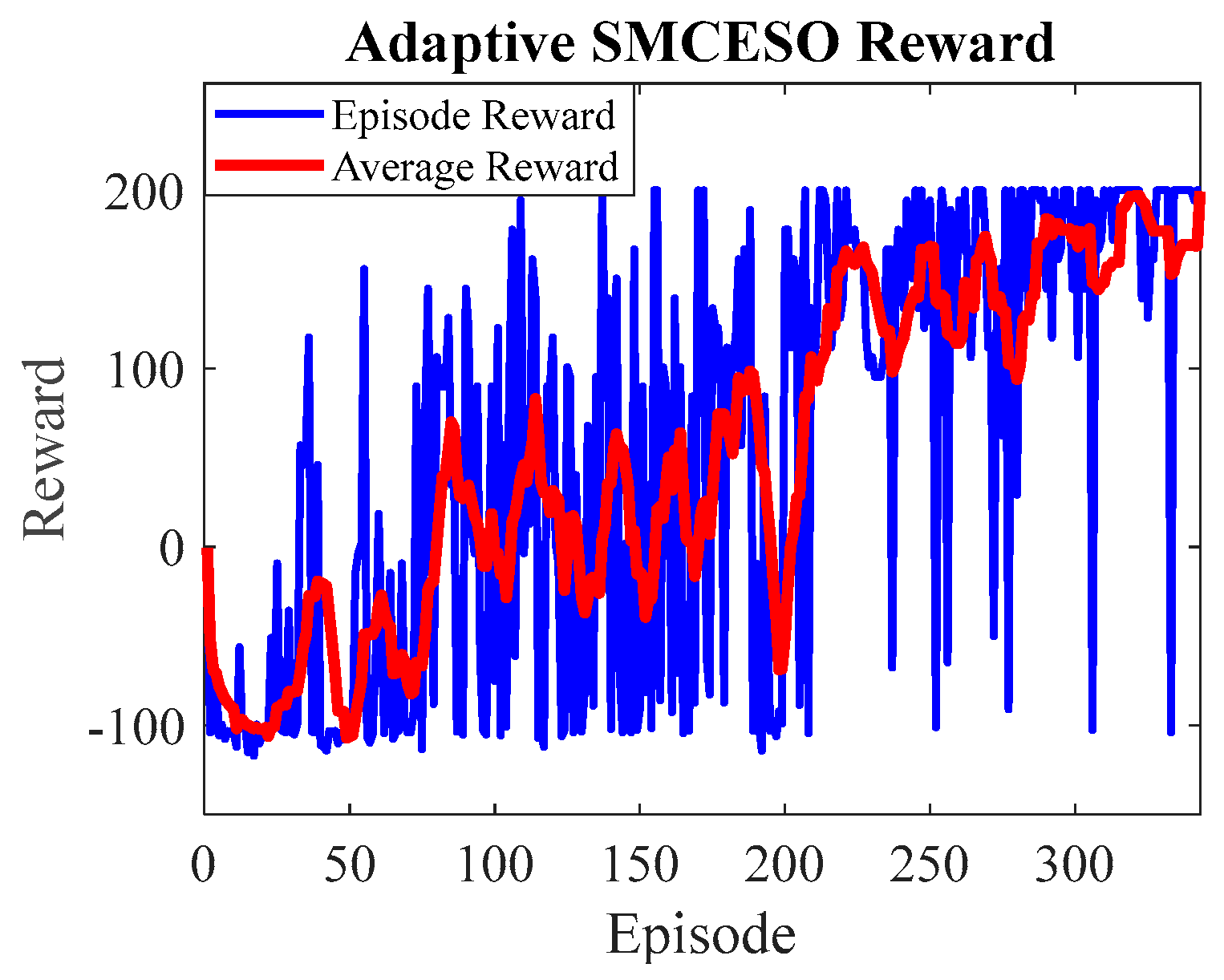
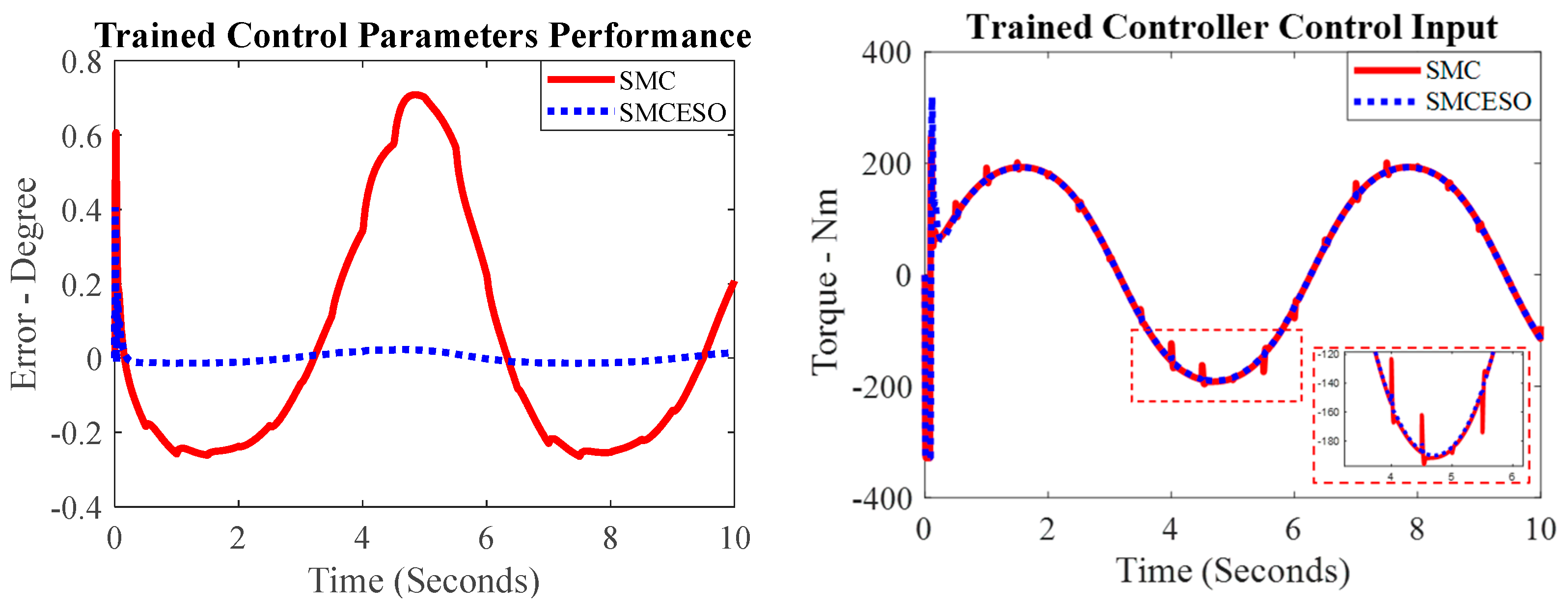
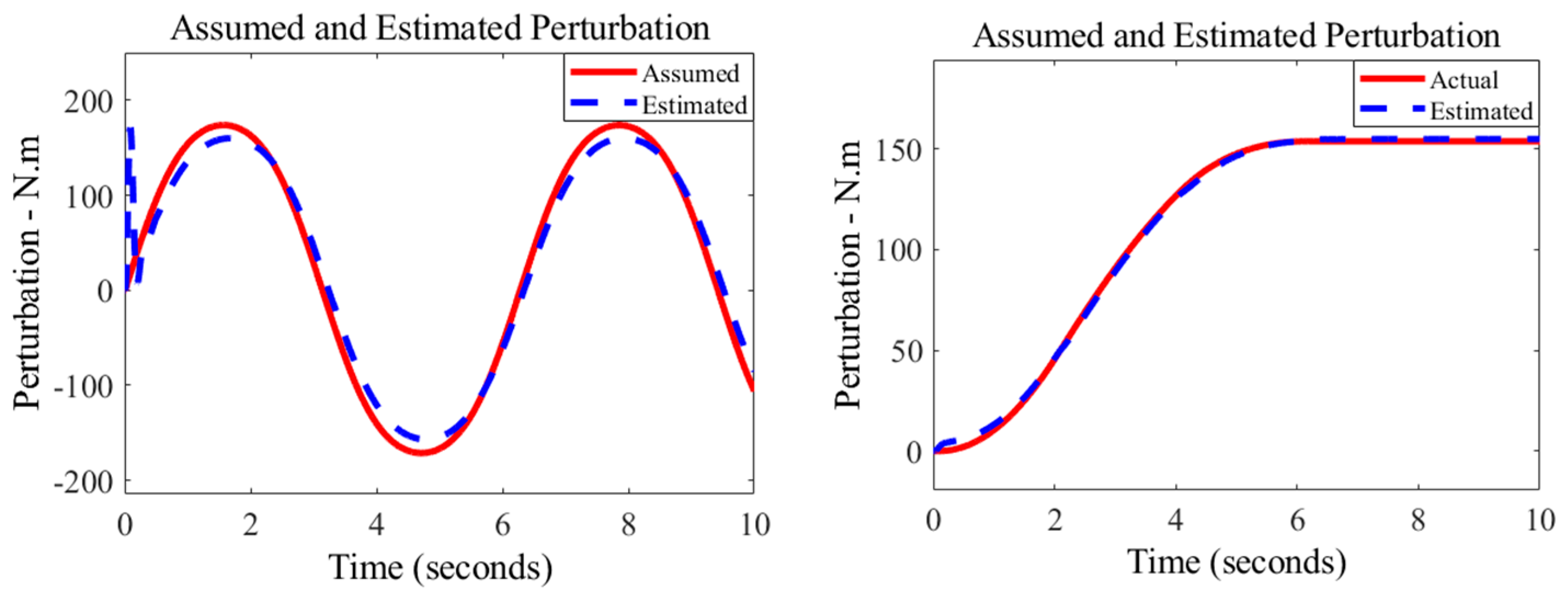
With a multibody robot system, the DDPG agent has been trained to fine-tune the controller parameters. For controller evaluation, Joint 2 ($q_2$) of the robot manipulator has been considered as it holds the maximum weight of the robot against gravity. Therefore, the robot arm is fully extended, and only $q_2$ is moving. The desired trajectory is defined as $q_{2,d}=\sin (w·t)$, with initial frequency $w_o=1$, which resets after every episode as $w=1+rand[-\mathrm{0.5,0.5}]$. Furthermore, the total simulation time is 10seconds, with an ideal reward $r_{max}=210$. The training stops when the average award reaches $r_c\ge 199$, considering the average reward window length. The DDPG agent took 343 episodes for the training. The episode reward and the cumulative reward are presented in the following Figure 5, and subsequently, the tuned parameters are shown in Figure 6 and the trajectory tracking error and joint torques are in Figure 7.

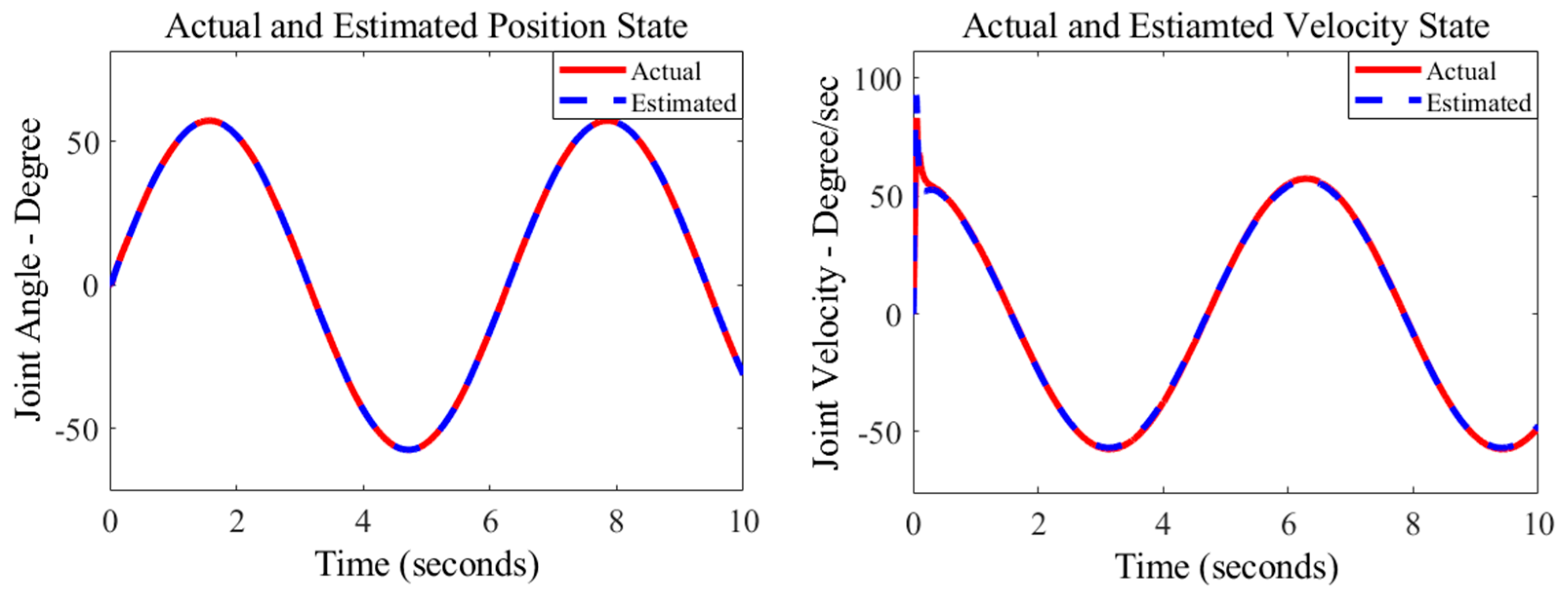
The joints were equipped with electromechanical motor dynamics with the motor parameters given in

Table 3. Motor dynamics parameters.

Parameter	Value
$\mathrm{Inductance}, L$	$0.573\times {10}^{-3} \mathrm{H}$
$\mathrm{Resistance}, R$	$0.978 \Omega$
$\mathrm{Torque} \mathrm{constant}, k_t$	$33.5\times {10}^{-3} \mathrm{N}·\mathrm{m}/\mathrm{A}$
$\mathrm{Voltage} \mathrm{constant}, k_e$	$33.5\times {10}^{-3} \mathrm{V}·\mathrm{s}/\mathrm{r}\mathrm{a}\mathrm{d}$
Gear Ratio	100

. Consequently, both control algorithms (SMC and SMCESO) can achieve joint tracking errors with the range $\pm 1 degree$. However, it is evident from the control input that SMC has sudden spikes throughout the simulation. Reducing gains can eliminate these spikes but will reduce the control performance, resulting in larger errors. Similarly, to reduce the error of SMC, higher gains (more than double those of SMCESO) are required. This, in turn, increases the spikes and occasionally introduces chattering in the response. In contrast, SMCESO shows very smooth performance and keeps the error within the range of $\pm 0.1 degree$. This validates the robustness of SMC integrated with ESO, which overcomes the perturbation effects of the system with a total mass $m>55 \mathrm{K}\mathrm{g}$ on joint 2. Overall, the initial jump in the control input is primarily attributed to motor dynamics such as friction, which stabilizes once the robot starts moving. Moreover, for a deeper understanding of achieving robust performance, observing the estimated states in Figure 8.

The position and velocity results show that the state observer is performing very well, with estimations showing nearly zero error. This suggests that the system may have highly effective perturbation estimation and compensation capabilities to enhance tracking performance. Moreover, the Simscape multibody toolbox allows obtaining the dynamics components of the robot system, including the mass matrix $M\left(q\right)$, velocity product torque $C\left(q,\dot{q}\right)·\dot{q}$ with $C\left(q,\dot{q}\right)$ Coriolis terms, and gravitational torque $G\left(q\right)$. This can be achieved through first creating the rigid body tree and then utilizing the Manipulator Algorithm library from Robotics System Toolbox. Subsequently, similar to (10), the expected perturbation is presumed as

$$\psi \left(x,t\right)=C\left(q,\dot{q}\right)·\dot{q}+G\left(q\right)$$

(40)

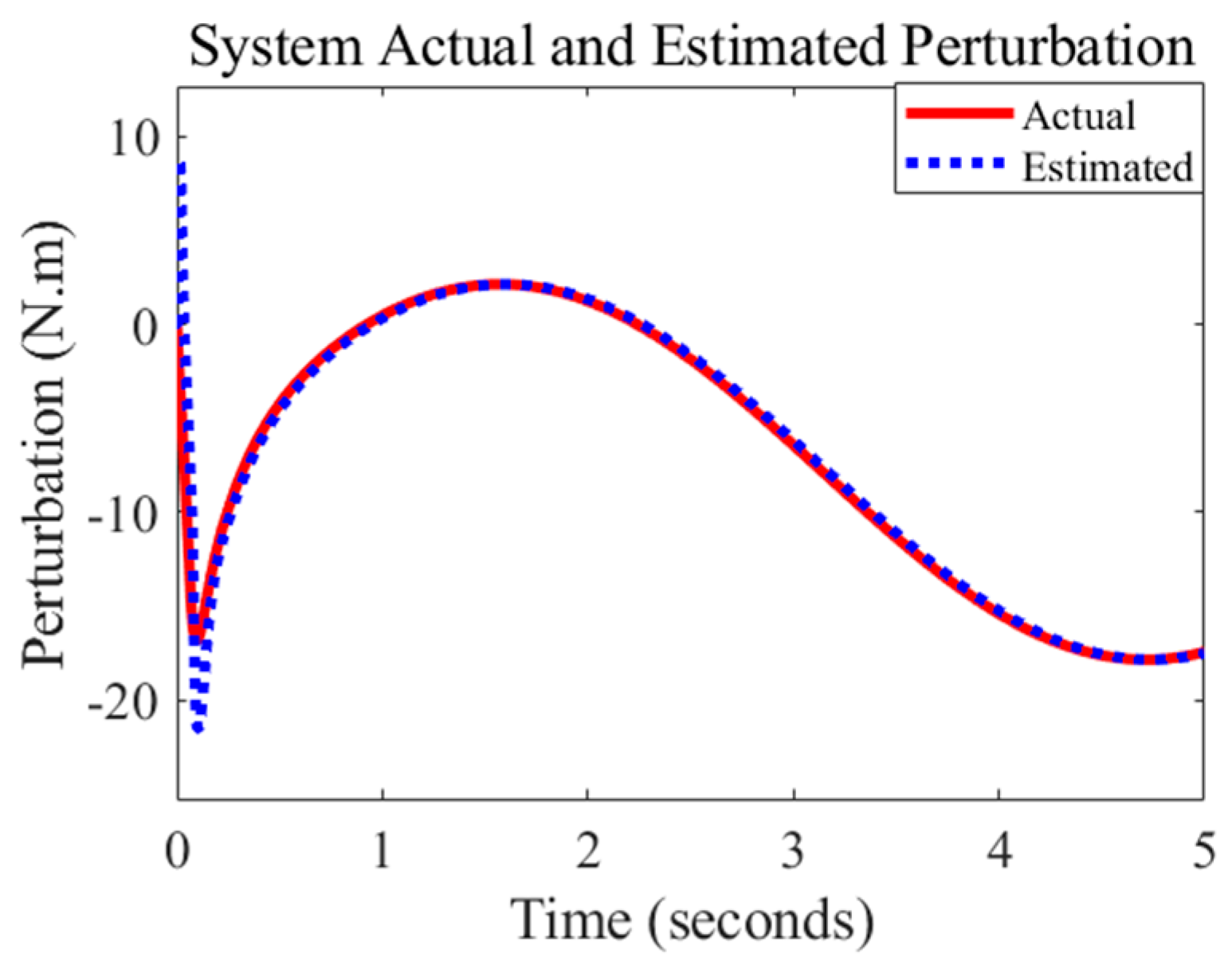
The assumed and estimated perturbations are presented in Figure 9, below.

The estimated perturbation closely aligns with the assumed perturbation. With the desired trajectory being a sine wave, the velocity is continuously changing, leading to some perturbation estimation error, as expected due to the motor dynamics, which are not factored into the perturbation calculation. However, this error can be compensated by the SMC in Equation (16), further validating the theory in Equation (29) that, with ESO, the system dynamics are primarily influenced by the perturbation estimation error. From a magnitude perspective, it is evident that the perturbation estimation error is considerably smaller than the actual perturbation, making the system achieve robust performance. Furthermore, when the robot comes to a stop, the estimated perturbation converges to match the assumed perturbation, confirming the accurate working of the ESO.

5. Conclusions

In this study, an approach to control and stabilize multibody robotic systems with inherent dynamics and uncertainties is presented. The approach leverages extended state observer (ESO) and sliding mode control (SMC) (SMCESO), combined with the optimization capabilities of deep deterministic policy gradients (DDPGs). One of the advantages of ESO is that it requires only partial state feedback (position) to estimate the perturbation, which includes the system dynamics and external disturbances. Initially, the proposed algorithm is implemented on a simple second-order system with introduced sinusoidal disturbance. Subsequently, the control parameters were fine-tuned using a DDPG agent, which was trained based on system tracking error, joint angle, estimated joint angle, and estimation error. This training allowed the DDPG-based SMCESO to outperform the optimally tuned PID control (via a control tuner toolbox), conventional SMC (tuned through DDPG), and $H_{\infty }$ control in terms of robustness, significantly enhancing system stability and performance. Even in the presence of disturbances, the SMCESO consistently converges to zero error due to its perturbation rejection capabilities. It was also demonstrated that with ESO, the system dynamics are primarily affected by the perturbation estimation error, which was validated through simulations showing close alignment between estimated and actual perturbations, leaving only minor estimation errors to be handled by the SMC control input. As a result, the multibody robot system’s overall performance is highly robust.

References

1. Shtessel, Y.; Edwards, C.; Fridman, L.; Levant, A. Introduction: Intuitive Theory of Sliding Mode Control. In Sliding Mode Control and Observation; Control Engineering; Birkhäuser: New York, NY, USA, 2014; pp. 1–42. [Google Scholar]
2. Afifa, R.; Ali, S.; Pervaiz, M.; Iqbal, J. Adaptive Backstepping Integral Sliding Mode Control of a MIMO Separately Excited Dc Motor. Robotics 2023, 12, 105. [Google Scholar] [CrossRef]
3. Khan, H.; Abbasi, S.J.; Lee, M.C. DPSO and Inverse Jacobian-based Real-time Inverse Kinematics with Trajectory Tracking using Integral SMC for Teleoperation. IEEE Access 2020, 8, 159622–159638. [Google Scholar] [CrossRef]
4. Hollweg, G.V.; de Oliveira Evald, P.J.; Milbradt, D.M.; Tambara, R.V.; Gründling, H.A. Design of continuous-time model reference adaptive and super-twisting sliding mode controller. Math. Comput. Simul. 2022, 201, 215–238. [Google Scholar] [CrossRef]
5. Mobayen, S.; Bayat, F.; ud Din, S.; Vu, M.T. Barrier function-based adaptive nonsingular terminal sliding mode control technique for a class of disturbed nonlinear systems. ISA Trans. 2023, 134, 481–496. [Google Scholar] [CrossRef] [PubMed]
6. Khan, H.; Abbasi, S.J.; Lee, M.C. Robust Position Control of Assistive Robot for Paraplegics. Int. J. Control Autom. Syst. 2021, 19, 3741–3752. [Google Scholar] [CrossRef]
7. Abbasi, S.J.; Khan, H.; Lee, J.W.; Salman, M.; Lee, M.C. Robust Control Design for Accurate Trajectory Tracking of Multi-Degree-of-Freedom Robot Manipulator in Virtual Simulator. IEEE Access 2022, 10, 17155–17168. [Google Scholar] [CrossRef]
8. Humaidi, A.J.; Hasan, A.F. Particle Swarm Optimization-Based Adaptive Super-Twisting Sliding Mode Control Design for 2-Degree-of-Freedom Helicopter. Meas. Control 2019, 52, 1403–1419. [Google Scholar] [CrossRef]
9. Wang, Y.; Zhu, K.; Yan, F.; Chen, B. Adaptive Super-Twisting Nonsingular Fast Terminal Sliding Mode Control for Cable-Driven Manipulators using Time-Delay Estimation. Adv. Eng. Softw. 2019, 128, 113–124. [Google Scholar] [CrossRef]
10. Wang, H.; Fang, L.; Song, T.; Xu, J.; Shen, H. Model-free Adaptive Sliding Mode Control with Adjustable Funnel Boundary for Robot Manipulators with Uncertainties. Rev. Sci. Instrum. 2021, 92, 065101. [Google Scholar] [CrossRef]
11. Xi, R.-D.; Xiao, X.; Ma, T.-N.; Yang, Z.-X. Adaptive Sliding Mode Disturbance Observer-Based Robust Control for Robot Manipulators Towards Assembly Assistance. IEEE Robot. Autom. Lett. 2022, 7, 6139–6146. [Google Scholar] [CrossRef]
12. Jing, C.; Xu, H.; Niu, X. Adaptive Sliding Mode Disturbance Rejection Control with Prescribed Performance for Robotic Manipulators. ISA Trans. 2019, 91, 41–51. [Google Scholar] [CrossRef]
13. Zhao, H.; Tao, B.; Ma, R.; Chen, B. Manipulator trajectory tracking based on adaptive fuzzy sliding mode control. Concurr. Comput. Pract. Exp. 2023, 35, e7620. [Google Scholar] [CrossRef]
14. Khan, H.; Lee, M.C. Extremum Seeking-Based Adaptive Sliding Mode Control with Sliding Perturbation Observer for Robot Manipulators. In Proceedings of the IEEE International Conference on Robotics and Automation (ICRA), London, UK, 29 May–2 June 2023; pp. 5284–5290. [Google Scholar]
15. Razmi, H.; Afshinfar, S. Neural Network-Based Adaptive Sliding Mode Control Design for Position and Attitude Control of a Quadrotor UAV. Aerosp. Sci. Technol. 2019, 91, 12–27. [Google Scholar] [CrossRef]
16. Chen, Z.; Huang, F.; Chen, W.; Zhang, W.; Sun, W.; Chen, J.; Zhu, S.; Gu, J. RBFNN-Based Adaptive Sliding Mode Control Design for Delayed Nonlinear Multilateral Telerobotic System with Cooperative Manipulation. IEEE Trans. Ind. Inform. 2020, 16, 1236–1247. [Google Scholar] [CrossRef]
17. Wang, D.; Shen, Y.; Sha, Q.; Li, G.; Kong, X.; Chen, G.; He, B. Adaptive DDPG Design-Based Sliding-Mode Control for Autonomous Underwater Vehicles at Different Speeds. In Proceedings of the IEEE Underwater Technology (UT), Kaohsiung, Taiwan, 16–19 April 2019; pp. 1–5. [Google Scholar]
18. Mosharafian, S.; Afzali, S.; Bao, Y.; Velni, J.M. A Deep Reinforcement Learning-Based Sliding Mode Control Design for Partially Known Nonlinear Systems. In Proceedings of the European Control Conference (ECC), London, UK, 12–15 July 2022; pp. 2241–2246. [Google Scholar]
19. Lei, C.; Zhu, Q. U-Model-Based Adaptive Sliding Mode Control using a Deep Deterministic Policy Gradient. Math. Probl. Eng. 2022, 2022, 8980664. [Google Scholar] [CrossRef]
20. Pantoja-Garcia, L.; Parra-Vega, V.; Garcia-Rodriguez, R.; Vázquez-García, C.E. A Novel Actor—Critic Motor Reinforcement Learning for Continuum Soft Robots. Robotics 2023, 12, 141. [Google Scholar] [CrossRef]
21. Abbasi, S.J.; Lee, S. Enhanced Trajectory Tracking via Disturbance-Observer-Based Modified Sliding Mode Control. Appl. Sci. 2023, 13, 8027. [Google Scholar] [CrossRef]
22. Raoufi, M.; Habibi, H.; Yazdani, A.; Wang, H. Robust Prescribed Trajectory Tracking Control of a Robot Manipulator Using Adaptive Finite-Time Sliding Mode and Extreme Learning Machine Method. Robotics 2022, 11, 111. [Google Scholar] [CrossRef]
23. Saleki, A.; Fateh, M.M. Model-free control of electrically driven robot manipulators using an extended state observer. Comput. Electr. Eng. 2020, 87, 106768. [Google Scholar] [CrossRef]
24. Zheng, Y.; Tao, J.; Sun, Q.; Zeng, X.; Sun, H.; Sun, M.; Chen, Z. DDPG-Based Active Disturbance Rejection 3D Path-Following Control for Powered Parafoil Under Wind Disturbances. Nonlinear Dyn. 2023, 111, 1–17. [Google Scholar] [CrossRef]
25. Sun, M.; Zhang, W.; Zhang, Y.; Luan, T.; Yuan, X.; Li, X. An Anti-Rolling Control Method of Rudder Fin System Based on ADRC Decoupling and DDPG Parameter Adjustment. Ocean. Eng. 2023, 278, 114306. [Google Scholar] [CrossRef]
26. Yang, J.; Peng, W.; Sun, C. A Learning Control Method of Automated Vehicle Platoon at Straight Path with DDPG-Based PID. Electronics 2021, 10, 2580. [Google Scholar] [CrossRef]
27. Dey, N.; Mondal, U.; Mondal, D. Design of a H-Infinity Robust Controller for a DC Servo Motor System. In Proceedings of the 2016 International Conference on Intelligent Control Power and Instrumentation (ICICPI), Kolkata, India, 21–23 October 2016; pp. 27–31. [Google Scholar]
Figure 1. Structure of DDPG.
Robotics 12 00161 g001
Figure 2. Block diagram of DDPG-based SMCESO.
Robotics 12 00161 g002
Figure 3. Controller performance evaluation: (a) with disturbance; (b) with parameter variation.
Robotics 12 00161 g003
Figure 4. Actual and estimated perturbation comparison.
Robotics 12 00161 g004
Figure 5. SMCESO training reward.
Robotics 12 00161 g005
Figure 6. SMCESO fine-tuned gains.
Robotics 12 00161 g006
Figure 7. Fine-tuned controller tracking performance.
Robotics 12 00161 g007
Figure 8. Actual and estimated states of the system.
Robotics 12 00161 g008
Figure 9. Perturbation results.
Robotics 12 00161 g009