Article

Dynamic and Friction Parameters of an Industrial Robot: Identification, Comparison and Repetitiveness Analysis

1
Department of Mechanical and Industrial Engineering, University of Brescia, Via Branze 38, 25123 Brescia, Italy
2
Istituto di Sistemi e Tecnologie Industriali per il Manifatturiero Avanzato, National Research Council (CNR-STIIMA), Via Corti 12, 20133 Milan, Italy
*
Authors to whom correspondence should be addressed.
Robotics 2021, 10(1), 49; https://doi.org/10.3390/robotics10010049
Submission received: 16 February 2021 / Revised: 16 March 2021 / Accepted: 17 March 2021 / Published: 19 March 2021
(This article belongs to the Section Industrial Robots and Automation)

Abstract

:
This paper describes the results of dynamic tests performed to study the robustness of a dynamics model of an industrial manipulator. The tests show that the joint friction changes during the robot operation. The variation can be identified in a double exponential law and thus the variation can be predicted. The variation is due to the heat generated by the friction. A model is used to estimate the temperature and related friction variation. Experimental data collected on two robots EFORT ER3A-C60 are presented and discussed. Repetitive tests performed on different days showed that the inertial and friction parameters can be robustly estimated and that the value of the measured joint friction can be used to estimate the unexpected conditions of the joints. Future applications may include sensorless identification of collisions, predictive maintenance programs, or human–robot interaction.

1. Introduction

The study of the dynamical performance of robotics machines is one of the most relevant problems in the design of effective robot control strategies. Parameter identification allows obtaining reliable dynamic models of industrial manipulators [1]. It is worth pointing out that a reliable dynamic model can improve position control [2]. Other applications may concern predictive maintenance, trajectory planning for energy efficiency [3], safety systems for robotic cells [4], or management of robot interaction with humans or the environment [5,6]. Many of these applications may require the knowledge of a good dynamic model of the robot. The robot’s dynamical parameters include inertial parameters (masses, centers of mass, and moments of inertia) and friction description. Joints and transmissions are considered rigid, which is acceptable for many industrial applications. The inertial parameters can be obtained by developing a model and by performing experiments on the robot. The authors of [7,8,9] showed that it is possible to define a set of parameters that describe the model (torque prediction) for any open-chain robot. The model is linear on these parameters and their regression matrix depends on the position, velocity, and acceleration of the joints. M. Gautier and W. Khalil proposed to drop the parameters that scarcely influence then fitting, obtaining a full-rank matrix. The remaining dynamical parameters involved in the identification are called the base parameters.
The identification process uses the Least Square Method, which provides reliable performance when models are linear in the parameters. During the test, the robot is moved on a properly designed excitation trajectory storing the position, velocity, acceleration, and torque of the joints. Then, the parameters that better predict the measured torques are estimated. Several criteria have been proposed to optimize the trajectory [10,11]. In this paper, the excitation trajectory is designed based on the finite Fourier series introduced by J. Swevers [12], with the benefit of data averaging in the time domain and reducing the measurement noise effect. An additional trajectory is appended to the excitation movement to guarantee the reaching of the joint-velocity bounds.
The linearity in the parameters does not hold in long time intervals, because the friction might change due to thermal effects. This model mismatch is evident comparing two experiments, one executed at the robot startup and one after the thermal transient. Friction is one of the most relevant undesired phenomena to be taken into account to realize a reliable dynamic model. It arises when there is a relative motion between two surfaces in contact or when a body moves inside a fluid. Friction depends on the geometry and the roughness of the surfaces, their materials, the type of lubricant, the velocity, the humidity, and so on [13]. Friction causes the loss of energy, heating of the surfaces in contact. This phenomenon introduces nonlinearities that might cause several problems related to motion control, such as trajectory tracking errors, limit cycles, and dynamic instabilities (stick-slip). For this reason, many friction models have been proposed in the technical literature (see [14]) to provide a suitable description of the physical phenomenon and to obtain effective mathematical formulations. These models can be classified into two main categories: static models and dynamic models.
The first category is simpler to analyze and concerns the models in which the friction force is a static function of the velocity. The most known static models are the Coulomb model, in which the friction action is considered constant and dependent only on the direction of the velocity, and the viscous friction, in which the force is proportional to velocity. Other models that belong to this category are the Stribeck model [15,16,17], in which an exponential function represents the transition between Coulomb and viscous friction, or the polynomial model, in which a polynomial expression is used to describe the relationship between friction force and velocity.
Regarding the dynamic models, on the other hand, the friction force depends on a state variable that takes into account the history of the system and not only its current situation. Relevant examples are the Dahl model [18], the Maxwell-slip model [19] and its extensions [20,21,22]. and the LuGre model [23,24,25]. In general, friction models are used in the control strategies to compensate for the friction effects (see [26,27]).
Despite the numerous efforts supported by research, this phenomenon is still a relevant issue for the control of industrial robots, and it depends on other factors than velocity. For this reason, some researchers started to focus on the role of temperature in friction [28,29,30]. Temperature is very important for those robot operations that require the manipulator to often stop for a long time, letting the joint temperature cool down and changing the friction characteristics. As explained in [31,32], friction transforms mechanical energy into heat, which causes a temperature increase [33], and therefore the behavior of the speed reducers changes too [34]. The installation of temperature sensors may be unpractical due to cost and compactness requirements. Thus, a possible solution to observe the relationship between friction and temperature could be based on the output of motor torque, which is easy to collect during the movement.
Opposite to friction parameters, inertial parameters should be independent of temperature, but a weak identification procedure and model mismatches may produce the wrong estimation of inertial parameters in function of the robot temperature. The same identification procedure can be carried out on multiple robots to verify the differences between machines and to verify the robustness of the identification. While papers generally discuss experimental data validated on one robot only, in this paper, we analyze multiple tests on two industrial robots (two replicas of the same model) to verify the repeatability of the results. This is important for establishing robust industrial applications. A comparison analysis allows understanding the differences between the dynamical and the friction behaviors changing among the robots. The results of the comparison would be useful for future improvement in manufacturing and maintaining of the machines. A further contribution of this paper is an analysis about the repetitiveness of the parameters estimation in several repetitions performed in different days and during the warming stage of the robot. The paper is organized as follows. Section 2 briefly describes the dynamics model of the manipulator. Then, the design of the excitation trajectory is presented. Section 3 deals with the analysis of the collected data and the estimated models. Discussions on results are in Section 4. Section 5 deals with the conclusion and future work.

2. Materials and Methods

The robots used during the experiments are the EFORT models ER3A-C60 located at the Robotics Laboratory of the University of Brescia. The two replicas are denoted simply as “Robot 1” and “Robot 2”. They are 6-DOF industrial manipulators with a maximum payload of 3 kg and a total weight of 27 kg. The identification of the dynamics model of the robotic arms can be divided into two sub-problems: the selection of a suitable model, the required parameters, and the mathematical method to identify them; and the design of a suitable excitation trajectory to collect meaningful data from the experimental campaign.

2.1. Dynamic Model and Parameters

As is known, the robot dynamic model can be obtained by a Lagrangian or Newton–Euler formulation [35], and it can be written as:
τ i n = M θ θ ¨ + V θ , θ ˙ + G θ
where θ , θ ˙ and θ ¨ are the joint position, velocity, and acceleration vectors, respectively. M ( θ ) is the mass matrix of robot arms, V θ , θ ˙ is the centrifugal and Coriolis force matrix and G θ is the gravity vector. τ i n is the torque components depending on masses, moments of inertia, and the centers of mass. It should be pointed out that the friction and the contribution of the external forces are not included. Thus, the full robot dynamical model is:
τ r o b o t = τ i n + τ f + τ e x t
where τ r o b o t is the torque output of each joint, τ f is the torque caused by friction, and τ e x t could be calculated knowing the Jacobian matrix and the external forces ( τ e x t = J T F e x t ), but it is assumed equal to zero in this work. To simplify the calculation, the model can be rewritten by reordering the terms of the equations; since the dynamic terms have a linear influence, the equation assumes the following matrix form:
τ r o b o t = K i n ψ i n + τ f = K i n ψ i n + K f ψ f = K i n K f ψ i n ψ f = K ψ
where K matrices, called information matrices, depend on θ , θ ˙ , and θ ¨ , and ψ vectors contain the dynamical parameters that need to be identified. More in detail, the subscript “ i n ” refers to the inertial parameters, while “f” refers to friction. In this paper, the vector ψ i n is the minimum set of dynamical parameters selected based on the linearization analysis [36], on numerical QR and singular value decomposition (SVD) factorizations [9], which benefit the computation cost. One of the mainly used friction models is based on the extended Coulomb models [37,38]. It might include the Stribeck effect [39], and it may assume the following polynomial form, which is a generalization of the Coulomb and viscous model:
τ f = k 1 s i g n θ ˙ + k 2 θ ˙ + k 3 θ ˙ 2 s i g n θ ˙ + k 4 θ ˙ 3
where τ f is the friction torque of one robot joint and the constants k 1 , k 2 , k 3 , and k 4 are parameters obtained with a identification. Their values changes with the temperature, as further explained in Section 2.3; s i g n θ ˙ is the sign function equal to 1 for positive velocity, 1 for negative velocity, and z e r o for null velocity. A three-order polynomial is generally sufficient to accurately describe the velocity-friction relation, so (4) describes the friction in function of speed and temperature.
Figure 1 shows the friction torque versus the joint velocity at different temperatures of the gearbox of one of the robots used in our tests. To find the numerical value of the constants k i , for an assigned temperature, the Least Square criterion is introduced. Least Square is the standard method to approach the solution of the linear system [40]. The main purpose of Least Square is to find the parameter values which minimize the sum of the square of the errors between the given data and estimated results. In practice, the robot can be moved on suitable joint trajectories and the motor torques can be collected at predefined sampling instants. Equation (3) can be written for each sampling time and all the equations can be combined into one. Therefore, with the given data P of n sampling points, the resulting equation is:
τ = τ p o i n t 1 τ p o i n t 2 τ p o i n t n = K 1 K 2 K n ψ = K ^ ψ
The least square estimation ψ ^ of ψ is then:
ψ ^ = K ^ T K ^ 1 K ^ T τ
To consider the joint friction changes, the estimation must be repeated at different joint temperature to identify the thermal model (see also Section 2.3).

2.2. Excitation Trajectory

A well-designed test trajectory has to excite the influence of all the model’s parameters and must include periods with large ranges of velocities from zero to high values. Since friction depends on joint temperatures, which changes during robot operation, the test trajectory must be sufficiently short to avoid altering the temperature significantly. To identify the dependency of the friction on temperature, the test is repeated during the time and it is alternated with special high-speed trajectories to warm up the joints. In this paper, to better identify friction and inertial parameters, the trajectories are divided into three stages: the first is optimized for inertial parameter estimation, the second is specially designed for friction estimation, and the third is a warming trajectory to prepare the next identification step. Figure 2 shows one of these trajectories; it should be noted that the friction identification is performed one joint at each time.
The portion of the trajectory responsible to estimate the inertial parameters has been designed to optimize the condition number of the information matrix [12] and has the following form:
θ i t = q i , 0 + l = 1 N a l , i w f l sin w f l t b l , i w f l cos w f l t
Each joint motion is defined as a constant plus a series of N sines and cosines whose amplitude and frequency are determined by an optimization algorithms. N was assumed equal to 5 because a higher number proved to be unnecessary (first part of Figure 3).
To be sure that all the joints reach the maximum velocity, an additional motion section was added. It is based on a cycloidal law, and it is reversed to assure it includes both positive and negative velocities. The initial and final points are coincident (second part of Figure 3). The trajectory equation is the following:
θ = θ 0 + Δ θ t t d 1 2 π sin 2 π t t d
θ ˙ = Δ θ t d 1 cos 2 π t t d
θ ¨ = 2 Δ θ t d 2 sin 2 π t t d
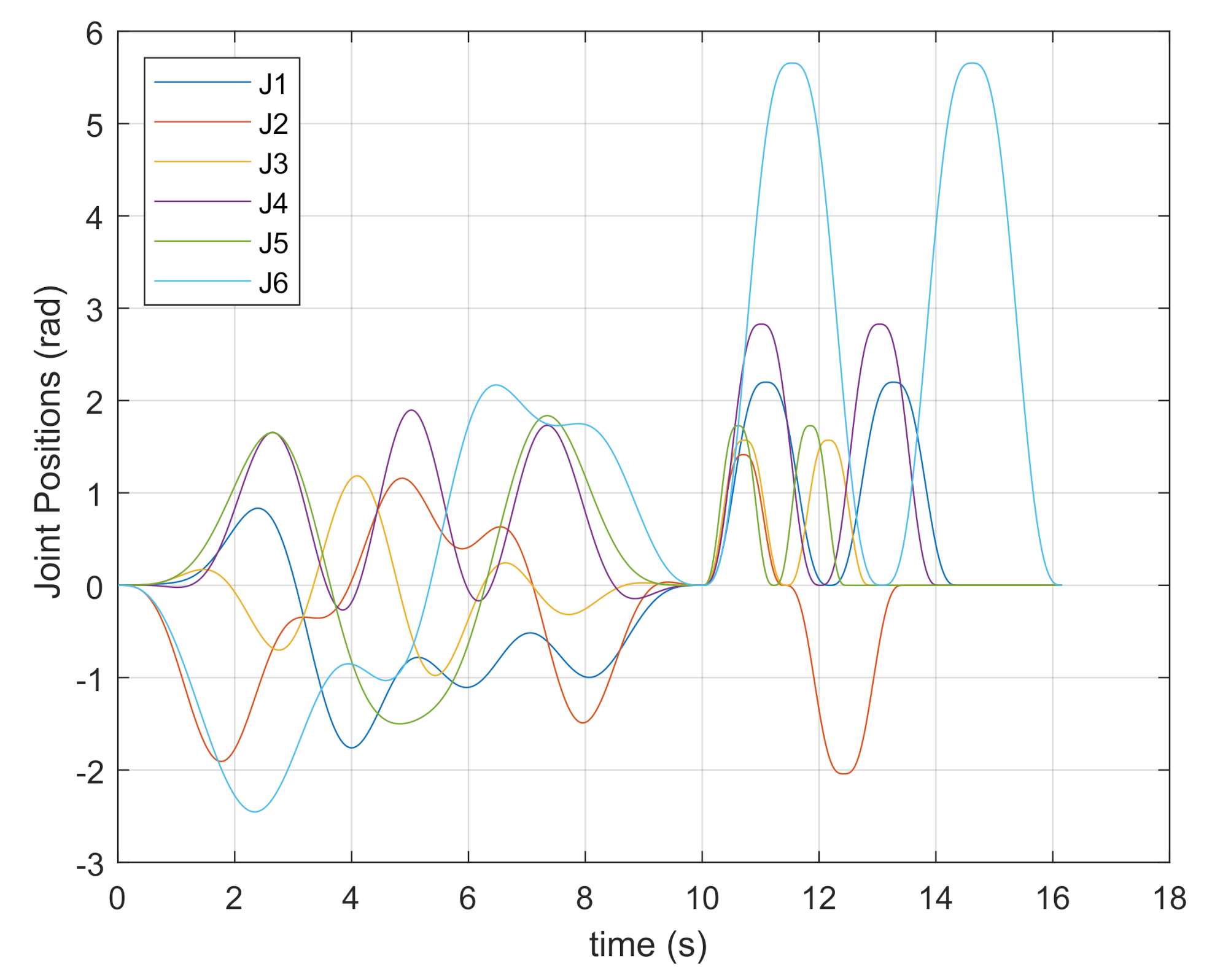
where Δ θ is the motion amplitude and t d is the time duration; these parameters were adjusted to reach the maximum velocity permitted by each joint. The final excitation trajectories are reported in Figure 3.
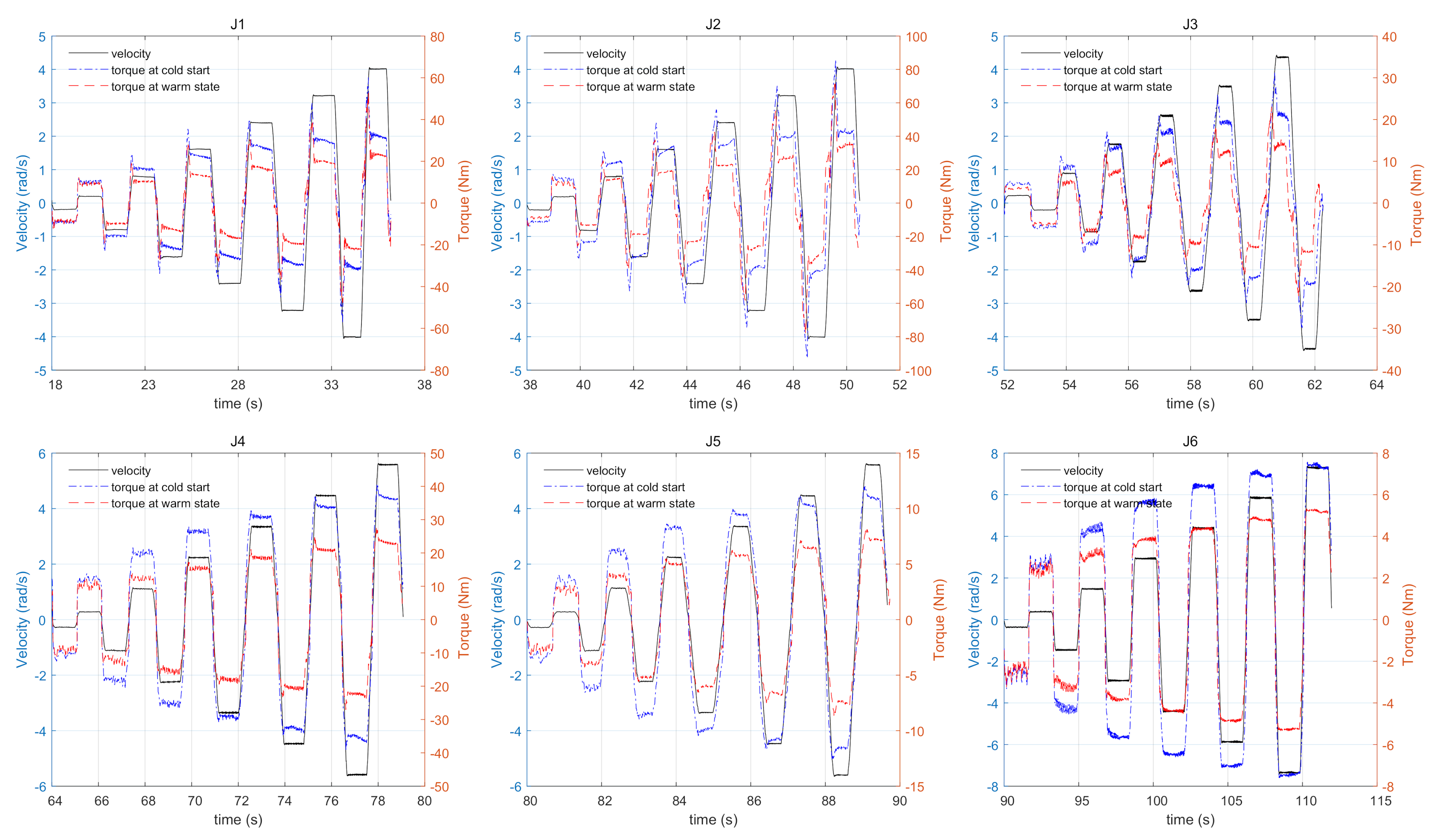
Since the duration of the trajectories is not identical for all joints, some idle periods were added. To measure the friction torque, which depends on speed, a special trajectory with six trapezoidal velocities was designed (see central section of Figure 2); each segment includes periods with a constant velocity at 5%, 20%, 40%, 60%, 80%, and 100% of the maximum joint velocity. The acceleration parts of the trajectory are ignored to avoid dynamics effects. The influence of the weight in the constant velocity periods was removed using the technique explained briefly below and in detail in [41]. To obtain the same number of data for each velocity all periods are equivalent and, consequently, the amplitude of the motion is bigger at the higher velocity. Both positive and negative velocities are included.
It should point out that the collected torque contains the gravitational component for some joints. To eliminate its effect, the robot was put into specific configurations so that the rotation axes of Joints 1, 4, 5, and 6 are vertical. For the remaining joints, Joints 2 and 3, the gravity effect was eliminated by a Least Squares procedure. During the motion at a constant velocity of an individual joint (see Figure 4), the motor torque is:
τ n o g r a v i t y = τ m o t o r P y cos θ P x sin θ
where P x and P y are the parameters to identify.
Once these parameters are determined, the gravity effects can be subtracted to obtain only the friction component. Examples of original data for Joints 2 and 3 are shown in Figure 5a). Figure 5b shows the same data after removing the gravity effect. The different curves represent the torque with different temperature of the joint. The tests were performed at 60% of the maximum velocity. The warming up of the joint is obtained by repeating movements at high speed that increases the internal temperature due to the power dissipated by the friction. This heating is achieved by running a robot working program with all joints moved simultaneously and repeatedly. Based on the experiments and the study of Pagani et al. [41], the first group of test cycles was performed at a temporal distance of about 3 min and the last group at a time interval of about 5 min. The merge of all the trajectory sections (inertial, friction, and warming) generates one cycle, which has a duration of 4.5 min roughly. To acquire enough data for the analysis, 24 cycles were performed, which correspond to about 2 h per experiment.

2.3. Temperature Effects

The friction parameters are highly dependent on temperature. The temperature of the gearbox is not available in most of the industrial robots in the market. Thus, it is necessary to estimate both the temperature and the thermal model from the experimental data. The estimation is possible by executing several warm-up tests with different root-mean-squared values of the joint torque, as proposed in [42] for a first-order thermal model and extended by Legnani et al. [43] for second-order models.
The second-order thermal model has two thermal capacities, which exchange heat linearly with the temperature differential. The exchanged heat with the environment is assumed linearly dependent on the temperature of the thermal capacities. Finally, the heat generated by friction is the product W f = τ f θ ˙ . Thus, the temperature evolves as described by the following transfer function:
T ( s ) W f ( s ) = c 1 s + τ 1 1 + c 2 s + τ 2 1
where s is the Laplace variable, T is the gearbox temperature, and τ 1 , τ 2 , c 1 , and c 2 are model parameters.
According to Pagani et al. [41], when one robot is actuated on a repetitive working cycle, sufficiently shorter than the time constants t 1 and t 2 , the joint temperatures changes as the step response of (12) where the heat is given by the root-mean-square value W f , r m s computed in the working cycle:
T = T 0 + c 1 τ 1 1 e t t 1 + c 2 τ 2 1 e t t 2 W f , r m s
where t is the time and T 0 is the initial temperature. Given an estimated temperature, the friction changes as:
τ f = τ 0 1 + α T T 0
where α is a constant dependent on the thermal model and τ 0 is friction torque at the initial temperature T 0 . By combining (4) with (14), we obtain a friction estimation formula as
τ f = 1 + α T T 0 k 1 s i g n θ ˙ + k 2 θ ˙ + k 3 θ ˙ 2 s i g n θ ˙ + k 4 θ ˙ 3
this relation is valid both for constant velocity situations as well as for transients, as described in Algorithm 1. Line 3 of the algorithm is the finite difference equation obtained by discretizing (12).
It is worth noticing that, in the special case of repetitive short cycles shown in Figure 6 and Figure 7, the friction torque changes as:
τ f = 1 + α W f , r m s c 1 τ 1 1 e t t 1 + c 2 τ 2 1 e t t 2 τ 0
Thanks to (13) and (15), it is possible to identify the parameters α , c 1 , c 2 , τ 1 , and τ 2 of the thermal model following the procedure described in [41], where a genetic algorithm tunes the model parameter to fit multiple warming cycles with different values of W f , r m s .
Algorithm 1:Evolution of the estimated temperature
Input: velocity θ ˙ ( k ) ; estimated temperature T ( k 1 ) and T ( k 2 ) at the steps k 1 and k 2 ; discretization period δ t
Output: estimated temperature T ( k ) at step k
τ f ( k ) = 1 + α T ( k 1 ) T 0 k 1 s i g n θ ˙ ( k ) + k 2 θ ( k ) ˙ + k 3 θ ˙ 2 ( k ) s i g n θ ˙ ( k ) + k 4 θ ˙ 3 ( k ) ;
W f ( k ) = τ f ( k ) θ ( k ) ˙ ;
T ( k ) = thermal model ( W f ( k ) , T ( k 1 ) , T ( k 2 ) , δ t ) ;
Figure 8 shows the complete model used in torque estimation. The dynamic model (3) uses the position, velocity, and acceleration of the joints and the measure of external force (if any) to estimated the actual torque. The friction component τ f uses the temperature prediction obtained by the thermal model thanks to Algorithm 1. A discrepancy between the estimation and the measured torque is inevitable; however, if this value is considerable, some other factor intervene: contacts with the environment or a malfunction of the mechanical transmissions. Specialized algorithms can deal with these situations (e.g., [44,45]).
The comparison between the estimated torque and the measured one can be the input of virtual force sensors, collision detectors, or maintenance supervisor.
It is worth pointing out that, once the thermal model is estimated, it is possible to use the actual friction torque to estimate the joint temperature when there are not unmeasured external forces acting on the robot employing a state observer [46].

2.4. Data Acquisition and Elaboration

Two robots of the same model EFFORT ER3A C-60 were used for the experiments, named “Robot 1” and “Robot 2”. The data acquisition was repeated four times for each robot on different days. To have comparable environmental conditions, all tests were executed in the morning after at least 8 h of robot rest and with an environmental temperature of about 20 C. For each movement, a PC-based acquisition system collected the motor’s positions and torques with a frequency of 4 ms. After the data collection, identification and analysis were developed using MATLAB programming environment. The data collected during all the repetitions of the 24 different cycles were analyzed to estimate inertial and friction parameters. Inertial parameters should be independent of the temperature and their numerical estimation would be expected to give constant results. The friction instead depends on temperature which increases with the robot activity, therefore a time-dependent trend with asymptotic behavior is expected for these parameters. The results show that the estimated dynamic parameters also had an asymptotic behavior; however, the range of the variation is generally minimal.
Examples of the results for inertial parameters are presented in Figure 9. The figure clearly shows that the estimated values of parameters change with cycles, but the variation is very little and the steady-state value is reached after about 15 cycles that correspond approximately to 1.5 h of the experiment. The coefficient k i of (4) change with behavior similar to (16). This trend is due to the model mismatches introduced by the thermal effect and the resulting identification error. In fact, the friction torque of Joint 3 at 60% of the velocity and its estimation are reported in Figure 6. It is worth pointing out that the friction torque at the cold state can be 70% higher than the final value, highlighting the relevance of the phenomenon.

3. Results

As first results, Figure 10 reports the different friction torque for different velocities in cold and hot conditions for the six joints. According to our experiments, the estimated temperature obtained by the thermal model could change from about 15 C (cold state) to about 50 or 60 C (depending on the joint) in hot state. Moreover, these values were confirmed by the data collected using temperature sensors located near the gears.
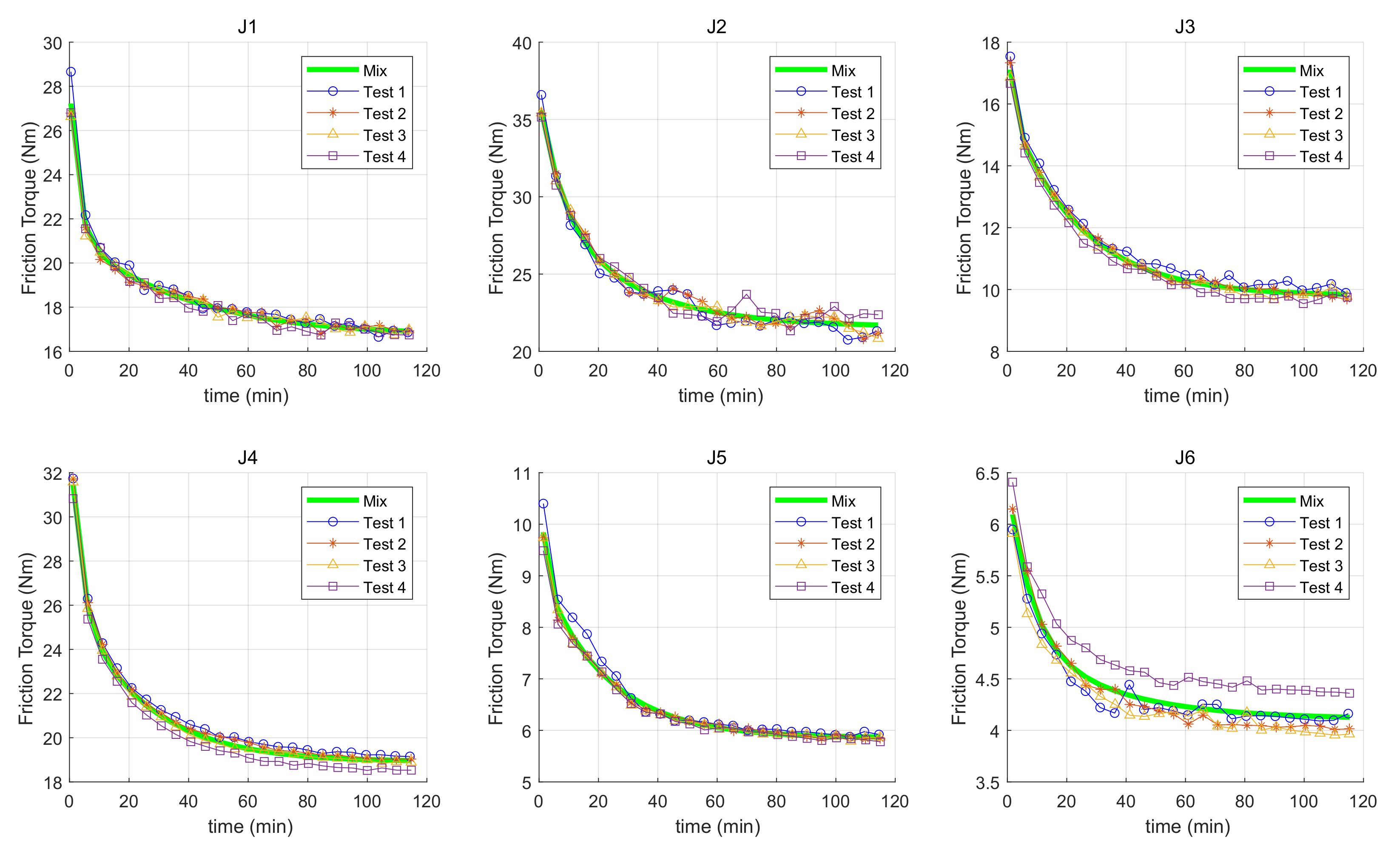
As stated in Section 2.4, the described analysis was applied to two manipulators of the same model named “Robot 1” and “Robot 2”. The two robots showed very similar behavior with the exception of the few cases mentioned in the paper and dependent on a mechanical problem in ”Robot 1”. The results of the friction estimation on ”Robot 1” for all the six joints at 60% of the maximum velocity are presented in Figure 7. The time constants of the curve fitting are reported in Table 1. The identification was performed for each test repetition as well as on the merge of the complete set of the collected data (mixed data). It is worth noting that the behavior of the robot is quite repetitive for all the joints. Each of them has regular heating which leads to a steady condition in about 1–2 h depending on the joint.
The time constant analysis of the six joints shows that one of them is shorter than the other one. While t 1 is in the range of 2–3 min, t 2 is in the range of 20–30 min, depending on the joint number. Moreover, Table 1 highlights that the different time constants estimation is mainly located at a narrow range for each joint. The Mix data are the results of curve fitting by merging the data of all tests. Based on the results of Figure 7, it is proved that the accuracy of the friction estimation is improved by the mixed data results. The estimation of the temperature during the working cycle permits predicting the correct friction contribution (see Figure 11 as an example).
The same procedure was implemented on ”Robot 2”. The results of the estimation on the friction-temperature characteristic are completely comparable to those obtained for ”Robot 1”. The curves exhibit similar trends and the ranges of the torque value are also equivalent. A further comparison between the two robots was performed on the estimation analysis of the inertial parameters. Results for some dynamic parameters are reported in Figure 12. The estimated values of these parameters for the two robots are reported for each of the 24 cycles. It is worth noting that they reach a stable value after a few cycles. The four repetitions of the test provide quite similar data. Thence, it is confirmed that the identification procedure is reasonably robust and suggests that the inertia parameters estimation can be performed after a short warming-up period of about 30–50 min (depending on the robot model).
The results obtained from these analyses show the repetitiveness of the experimental procedure used in this work. The parameters identified by the model are comparable between the tests carried out on different days and also comparable with those obtained on different robots but of the same model. It is of utmost importance to obtain a mathematical model describing the joints torques variations taking into account the temperature alterations that may occur during the working operation. This could be useful for multiple applications, such as predictive maintenance, advanced control strategies, the realization of virtual force sensors, and human–robot interaction. Figure 13 shows a clear example of the model implementation for predictive maintenance. During one of the tests carried out on “Robot 2”, a mechanical problem was found in the first joint. After about 60 min on the second day of the tests, the friction torque had an unexpected increase and then it settled at a higher value compared with the previous tests. The measurement carried out the day after shows that the same movement required more energy from the very start. A possible explanation for this phenomenon may be a mechanical problem inside the transmission. In this specific case, to restore the correct operation of the machine, it was sufficient to execute the inspection of the joint following the mechanical maintenance manual provided by the manufacturer. Further analysis of this issue is shown at the bottom of Figure 12. It is possible to note how the unexpected increase in friction torque results in a sudden change in the friction parameters of the dynamic model. The phenomenon just described suggests how the model provided in this work may be used for the preventive maintenance of industrial manipulators. By carrying out the identification procedure on a new robot, it is possible to obtain an initial condition state of the machine. Repeating this procedure over time, it is possible to compare the new results with the initial ones to check if the components have been damaged, helping the user to perform the necessary maintenance. It is worth pointing out that the unexpected increase is about the 32% of the expected value, while the change due to thermal effect is 60%/70%, thus the damage cannot be detected by using a model that neglects the thermal effect.

4. Discussion

The experimental campaign lasted several days using two robots of the same kind. The experimental data show the repeatability of the thermal phenomenon and the robust identification of the parameters of the dynamics and thermal models.
This repeatability allows detecting unforeseen changes of the friction torque due to minor mechanical damages, as shown in Figure 13. It is worth stressing that the friction changes from cold to warm conditions are more significant than the changes due to the damages. Thus, one of the main advantages of integrating a thermal model is to provide a higher discrimination level than models that neglect temperature effects, allowing early detections of torque changes due to aging and damages.
Another advantage of the algorithm is the ability to predict the required torque, improving the performance of control algorithms based on precomputed torque.
The main drawback is the requirement of an extended test campaign on a representative batch of each robot type.

5. Conclusions

The study of the robot dynamics and, in particular, the friction torques is crucial to understand the robot behavior, as mentioned in the Introduction. This information is helpful to analyze the aging and appearance of possible defects during the robot activities. As is well known, the design of a suitable exciting trajectory is essential to estimate the robot parameters correctly.
The paper shows the effectiveness of the dynamics model, coupled with the temperature-based friction model, to match experimental data in multiple robots. The experimental campaign, performed on several days, showed consistent results. The paper shows that the estimated parameters are biased during the first part of the thermal transient due to friction changes. Thus, a model that neglects temperature effects can work properly if and only if the model is identified and used at the same thermal steady-state. Otherwise, a temperature estimator is required to compensate for its effect.
Therefore, this paper could help people understand the robot behavior changes during working cycles and develop a dynamic model of the robot, including the thermal effect.
The model can effectively estimate the friction variation due to temperature. Since this variation is up to 70%, it is crucial to consider it in the torque estimation to discriminate it from other changes due to possible damages or aging. It is worth pointing out that this discrimination ability could be relevant in advanced maintenance and performance monitor.
Future works will deal with the study and the identification procedure of the thermal effects on the friction at lower velocities, the possible usage of the proposed model in maintenance and performance monitoring scenarios.

Author Contributions

Conceptualization, G.L., M.B. and R.P.; methodology, R.P. and L.H.; software, L.H.; validation, L.H., and R.P.; formal analysis, R.P.; writing—original draft preparation, L.H.; writing—review and editing, R.P.; visualization, G.L. and M.B.; supervision, G.L.; and project administration, G.L. All authors have read and agreed to the published version of the manuscript.

Funding

This research received no external funding.

Acknowledgments

The authors thank Evolut Spa, Brescia (IT), Robox Spa, Novara (IT) and Efort Intelligent Equipment Co. Ldt, Wuhu, China (CN) for the support during the research activity.

Conflicts of Interest

The authors declare no conflict of interest.

References

  1. Beschi, M.; Villagrossi, E.; Pedrocchi, N.; Tosatti, L.M. A general analytical procedure for robot dynamic model reduction. In Proceedings of the 2015 IEEE/RSJ International Conference on Intelligent Robots and Systems (IROS), Hamburg, Germany, 28 September–2 October 2015; IEEE: New York, NY, USA, 2015; pp. 4127–4132. [Google Scholar]
  2. Khosla, P.K.; Kanade, T. Real-time implementation and evaluation of the computed-torque scheme. IEEE Trans. Robot. Autom. 1989, 5, 245–253. [Google Scholar] [CrossRef] [Green Version]
  3. Carabin, G.; Scalera, L. On the Trajectory Planning for Energy Efficiency in Industrial Robotic Systems. Robotics 2020, 9, 89. [Google Scholar] [CrossRef]
  4. Pasinetti, S.; Nuzzi, C.; Lancini, M.; Sansoni, G.; Docchio, F.; Fornaser, A. Development and characterization of a safety system for robotic cells based on multiple Time of Flight (TOF) cameras and point cloud analysis. In Proceedings of the 2018 Workshop on Metrology for Industry 4.0 and IoT, Brescia, Italy, 16–18 April 2018; IEEE: New York, NY, USA, 2018; pp. 1–6. [Google Scholar]
  5. Matheson, E.; Minto, R.; Zampieri, E.G.; Faccio, M.; Rosati, G. Human–Robot Collaboration in Manufacturing Applications: A Review. Robotics 2019, 8, 100. [Google Scholar] [CrossRef] [Green Version]
  6. Cannan, J.; Hu, H. Human-Machine Interaction (HMI): A Survey; University of Essex: Colchester, UK, 2011. [Google Scholar]
  7. Gautier, M.; Khalil, W. Direct calculation of minimum set of inertial parameters of serial robots. IEEE Trans. Robot. Autom. 1990, 6, 368–373. [Google Scholar] [CrossRef] [Green Version]
  8. Gautier, M.; Khalil, W. Identification of the minimum inertial parameters of robots. In Proceedings of the 1989 IEEE International Conference on Robotics and Automation, Scottsdale, AZ, USA, 14–19 May 1989; IEEE: New York, NY, USA, 1989; pp. 1529–1530. [Google Scholar]
  9. Gautier, M. Numerical calculation of the base inertial parameters of robots. J. Robot. Syst. 1991, 8, 485–506. [Google Scholar] [CrossRef]
  10. Swevers, J.; Ganseman, C.; Tukel, D.B.; De Schutter, J.; Van Brussel, H. Optimal robot excitation and identification. IEEE Trans. Robot. Autom. 1997, 13, 730–740. [Google Scholar] [CrossRef] [Green Version]
  11. Villagrossi, E.; Legnani, G.; Pedrocchi, N.; Vicentini, F.; Tosatti, L.M.; Abbà, F.; Bottero, A. Robot dynamic model identification through excitation trajectories minimizing the correlation influence among essential parameters. In Proceedings of the 2014 11th International Conference on Informatics in Control, Automation and Robotics (ICINCO), Vienna, Austria, 1–3 September 2014; IEEE: New York, NY, USA, 2014; Volume 2, pp. 475–482. [Google Scholar]
  12. Swevers, J.; Ganseman, C.; De Schutter, J.; Van Brussel, H. Generation of periodic trajectories for optimal robot excitation. J. Manuf. Sci. Eng. 1997, 119, 611–615. [Google Scholar] [CrossRef]
  13. Márton, L.; van der Linden, F. Temperature dependent friction estimation: Application to lubricant health monitoring. Mechatronics 2012, 22, 1078–1084. [Google Scholar] [CrossRef]
  14. Andersson, S.; Söderberg, A.; Björklund, S. Friction models for sliding dry, boundary and mixed lubricated contacts. Tribol. Int. 2007, 40, 580–587. [Google Scholar] [CrossRef]
  15. Stribeck, R. Kugellager für beliebige belastungen (ball bearings for arbitrary loads). In Mitteilungen aus der Centralstelle für wissenschaftlichtechnische Untersuchungen; HS Hermann: Berlin, Germany, 1900. [Google Scholar]
  16. Stribeck, R. Die wesentlichen eigenschaften der gleit-und rollenlager. Z. Des Vereines Dtsch. Ingenieure 1902, 46, 1341–1348. [Google Scholar]
  17. Simoni, L.; Beschi, M.; Legnani, G.; Visioli, A. On the inclusion of temperature in the friction model of industrial robots. IFAC-PapersOnLine 2017, 50, 3482–3487. [Google Scholar] [CrossRef]
  18. Dahl, P.R. A Solid Friction Model; Technical Report; Aerospace Corp El Segundo Ca: El Segundo, CA, USA, 1968. [Google Scholar]
  19. Lampaert, V.; Al-Bender, F.; Swevers, J. A generalized Maxwell-slip friction model appropriate for control purposes. In Proceedings of the 2003 IEEE International Workshop on Workload Characterization (IEEE Cat. No. 03EX775), St. Petersburg, Russia, 20–22 August 2003; IEEE: New York, NY, USA, 2003; Volume 4, pp. 1170–1177. [Google Scholar]
  20. Ruderman, M. Presliding hysteresis damping of LuGre and Maxwell-slip friction models. Mechatronics 2015, 30, 225–230. [Google Scholar] [CrossRef]
  21. Ferretti, G.; Magnani, G.; Rocco, P. Single and multistate integral friction models. IEEE Trans. Autom. Control 2004, 49, 2292–2297. [Google Scholar] [CrossRef]
  22. Piatkowski, T. GMS friction model approximation. Mech. Mach. Theory 2014, 75, 1–11. [Google Scholar] [CrossRef]
  23. Freidovich, L.; Robertsson, A.; Shiriaev, A.; Johansson, R. LuGre-model-based friction compensation. IEEE Trans. Control Syst. Technol. 2009, 18, 194–200. [Google Scholar] [CrossRef]
  24. De Wit, C.C.; Olsson, H.; Astrom, K.J.; Lischinsky, P. A new model for control of systems with friction. IEEE Trans. Autom. Control 1995, 40, 419–425. [Google Scholar] [CrossRef] [Green Version]
  25. Johanastrom, K.; Canudas-De-Wit, C. Revisiting the LuGre friction model. IEEE Control Syst. Mag. 2008, 28, 101–114. [Google Scholar] [CrossRef] [Green Version]
  26. Mallon, N.; van de Wouw, N.; Putra, D.; Nijmeijer, H. Friction compensation in a controlled one-link robot using a reduced-order observer. IEEE Trans. Control Syst. Technol. 2006, 14, 374–383. [Google Scholar] [CrossRef] [Green Version]
  27. Yoon, J.Y.; Trumper, D.L. Friction modeling, identification, and compensation based on friction hysteresis and Dahl resonance. Mechatronics 2014, 24, 734–741. [Google Scholar] [CrossRef]
  28. Bittencourt, A.C.; Wernholt, E.; Sander-Tavallaey, S.; Brogårdh, T. An extended friction model to capture load and temperature effects in robot joints. In Proceedings of the 2010 IEEE/RSJ International Conference on Intelligent Robots and Systems, Taipei, Taiwan, 18–22 October 2010; IEEE: New York, NY, USA, 2010; pp. 6161–6167. [Google Scholar]
  29. Bittencourt, A.C.; Axelsson, P. Modeling and experiment design for identification of wear in a robot joint under load and temperature uncertainties based on friction data. IEEE/ASME Trans. Mechatronics 2013, 19, 1694–1706. [Google Scholar] [CrossRef]
  30. Bittencourt, A.C.; Gunnarsson, S. Static friction in a robot joint—modeling and identification of load and temperature effects. J. Dyn. Syst. Meas. Control 2012, 134, 051013. [Google Scholar] [CrossRef]
  31. Pirro, D.M.; Webster, M.; Daschner, E. Lubrication Fundamentals, Revised and Expanded; CRC Press: Boca Raton, FL, USA, 2016. [Google Scholar]
  32. Neubauer, M.; Gattringer, H.; Bremer, H. A persistent method for parameter identification of a seven-axes manipulator. Robotica 2015, 33, 1099. [Google Scholar] [CrossRef]
  33. Bhushan, B. Frictional heating and contact temperatures. In Modern Tribology Handbook, Two Volume Set; CRC Press: Boca Raton, FL, USA, 2000; pp. 257–294. [Google Scholar]
  34. Zhao, Z. The Study of Friction Variation with Temperature in a Harmonic Drive System: Modeling and Control. Ph.D. Thesis, Concordia University, Concordia, KS, USA, 2006. [Google Scholar]
  35. Craig, J.J. Introduction to Robotics: Mechanics and Control, 3rd ed. Available online: https://www.pearson.com/us/higher-education/product/Craig-Introduction-to-Robotics-Mechanics-and-Control-3rd-Edition/9780201543612.html (accessed on 18 March 2021).
  36. Khalil, W.; Dombre, E. Modeling, Identification and Control of Robots; Butterworth-Heinemann: Oxford, UK, 2004. [Google Scholar]
  37. Liu, Y.; Li, J.; Zhang, Z.; Hu, X.; Zhang, W. Experimental comparison of five friction models on the same test-bed of the micro stick-slip motion system. Mech. Sci. 2015, 6, 15. [Google Scholar] [CrossRef] [Green Version]
  38. Simoni, L.; Beschi, M.; Legnani, G.; Visioli, A. Modelling the temperature in joint friction of industrial manipulators. Robotica 2019, 37, 906–927. [Google Scholar] [CrossRef] [Green Version]
  39. Armstrong-Helouvry, B. Stick slip and control in low-speed motion. IEEE Trans. Autom. Control 1993, 38, 1483–1496. [Google Scholar] [CrossRef]
  40. Grisetti, G.; Guadagnino, T.; Aloise, I.; Colosi, M.; Della Corte, B.; Schlegel, D. Least Squares Optimization: From Theory to Practice. arXiv 2020, arXiv:2002.11051. [Google Scholar] [CrossRef]
  41. Pagani, R.; Legnani, G.; Incerti, G.; Gheza, M. Evaluation and Modeling of the Friction in Robotic Joints Considering Thermal Effects. J. Mech. Robot. 2020, 12, 021108. [Google Scholar] [CrossRef]
  42. Legnani, G.; Simoni, L.; Beschi, M.; Visioli, A. A new friction model for mechanical transmissions considering joint temperature. In International Design Engineering Technical Conferences and Computers and Information in Engineering Conference; American Society of Mechanical Engineers: New York, NY, USA, 2016; Volume 50183, p. V006T09A020. [Google Scholar]
  43. Legnani, G.; Incerti, G.; Pagani, R.; Gheza, M. Modelling and Evaluation of the Friction in Robotic Joints Considering Thermal Effects. In International Design Engineering Technical Conferences and Computers and Information in Engineering Conference; American Society of Mechanical Engineers: New York, NY, USA, 2019; Volume 59230, p. V05AT07A062. [Google Scholar]
  44. Flores, P.; Ambrósio, J. On the contact detection for contact-impact analysis in multibody systems. Multibody Syst. Dyn. 2010, 24, 103–122. [Google Scholar] [CrossRef] [Green Version]
  45. Slamani, M.; Bonev, I.A. Characterization and experimental evaluation of gear transmission errors in an industrial robot. Ind. Robot Int. J. 2013, 40, 441–449. [Google Scholar] [CrossRef]
  46. Villagrossi, E.; Simoni, L.; Beschi, M.; Pedrocchi, N.; Marini, A.; Tosatti, L.M.; Visioli, A. A virtual force sensor for interaction tasks with conventional industrial robots. Mechatronics 2018, 50, 78–86. [Google Scholar] [CrossRef]
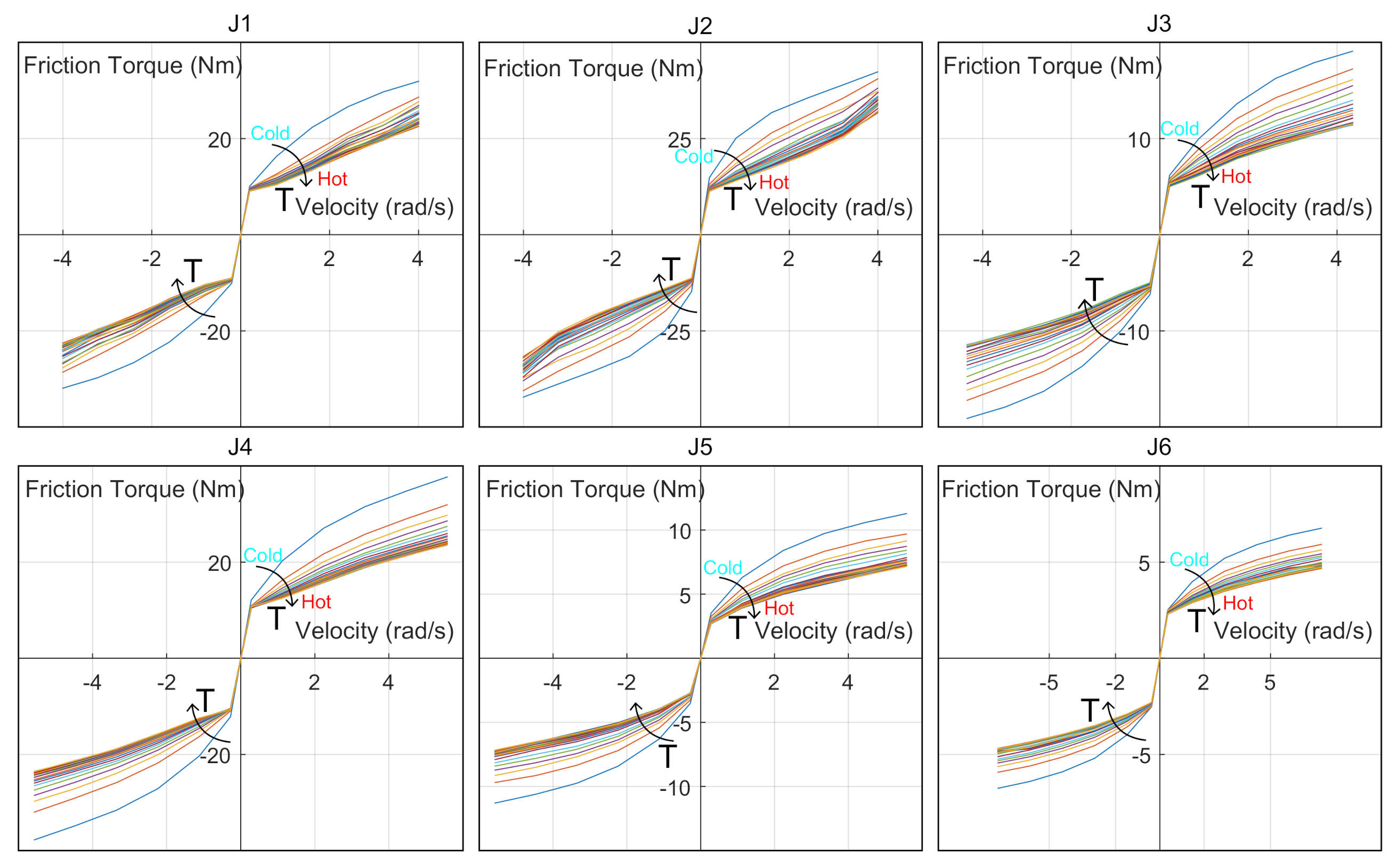
Figure 1. Friction versus speed changes as the robot warms up for each joint.
Robotics 10 00049 g001
Figure 2. One cycle of the test trajectory on all joints. The first section is reserved for the estimation of the inertial parameters. The second one is specially designed for friction estimation; the joints are moved individually one after the other to highlight the contribution of the friction component in the motor output. The last section takes care of heating the joints by performing a high-speed point-to-point movement for a few minutes.
Robotics 10 00049 g002
Figure 3. Position performed by each joint during the execution of the final excitation trajectory.
Robotics 10 00049 g003
Figure 4. Principle used for the simplified model of (11) when just one joint is moved at each time and the others assume a predefined value (example of Joint 2) The robot in the figure is the 3D model of the manipulator used in this work.
Robotics 10 00049 g004
Figure 5. Experimental data. (a) The torque motor output of Joints 2 and 3 during the friction measure cycle. Data collected from one test on “Robot 1” (60% of the velocity). (b) The same data without the gravity effect.
Robotics 10 00049 g005
Figure 6. (a) Mean value of friction torque versus time for each test on “Robot 1”. Experimental data, Joint 3, and velocity at 60%. (b) Fitting of the data using (16).
Robotics 10 00049 g006
Figure 7. Friction torque versus time for all joints in Tests 1–4 performed on “Robot 1”, with the velocity at 60%. The Mix curve is the results of the curve fitting by merging the data of each test. Joint 6 had a variation on Day 4, probably due to a measurement error, but the reason is under analysis.
Robotics 10 00049 g007
Figure 8. Scheme of the interconnections between the dynamic, the friction, and the thermal model and the possible use for advanced applications (predictive maintenance, virtual force sensor [46], and human–robot interaction). Symbols with the “hat” marks the estimated values, symbols without the “hat” are real values.
Robotics 10 00049 g008
Figure 9. Experimental data. (a) Evolution of the identified values P y of Joint 3 for all the tests on “Robot 2”. (b) The evolution of the same parameter, but slightly widening the scale of the value. It is worth noting that the difference between the initial and final estimations is less than 5%.
Robotics 10 00049 g009
Figure 10. Velocity and torque versus time during a working cycle in cold and hot conditions: experimental data for all 6 Joints.
Robotics 10 00049 g010
Figure 11. Example of measured and predicted torque (dynamics plus friction) in cold and hot conditions on the same trajectory with variable velocity (Joint 5, Test 1).
Robotics 10 00049 g011
Figure 12. Evolution of the identified values I x x , I x y , I x z , I y z , and I z z of Joint 2 for all the tests on “Robot 1” and “Robot 2”. The values of the parameters are repeatable and quite similar between the two robots.
Robotics 10 00049 g012
Figure 13. (Top) The friction torque versus time for “Robot 1” and “Robot 2”. During one of the tests on “Robot 2”, a mechanical problem occurred. It is possible to see the unexpected increase in torque on the left-side graph. The graph on the opposite side shows the ordinary behavior of “Robot 1” performing the same tests. (Bottom) The evolution of the friction parameters (Equation (4)) during the tests performed on “Robot 2”. It is evident how the mechanical problem results in a change in the model values.
Robotics 10 00049 g013
Table 1. Time constants (experimental estimation) of “Robot 1”.
Time Constants
[minutes]
Joint 1Joint 2Joint 3Joint 4Joint 5Joint 6
t 1 Test 12.72250.86600.57443.76500.25170.3447
Test 22.55670.37590.38433.70300.25178.1392
Test 31.69650.27641.72282.99692.03693.4120
Test 42.63490.24111.69352.79380.35012.9116
Mix2.44650.29490.91723.31090.32547.9114
t 2 Test 135.240216.667422.742925.891520.285212.4031
Test 238.972418.278524.598225.789120.285227.4701
Test 335.108817.082224.106322.433721.196725.4714
Test 433.073018.198023.365222.825321.911319.5745
Mix35.442417.010723.718724.056620.652932.5835
Publisher’s Note: MDPI stays neutral with regard to jurisdictional claims in published maps and institutional affiliations.