1. Introduction
With the advancement of technology and the invention of new wheels with special structures, omnidirectional mobile robots (OMRs) have been presented and widely used recently in industrial applications, space exploration, medical fields etc. [
1,
2,
3]. In spite of conventional mobile robots that use two driver wheels to control the robot motion on restricted directions, OMRs are not limited by nonholonomic constraints and can move in any direction from every configuration [
4]. This characteristic increases the maneuverability, swiftness and accuracy of the mobile robot, which makes the robot capable of working in small workspaces and dynamic environments with high precision [
5].
The dynamics and control of OMRs with different types and numbers of omni wheels have attracted several researchers recently due to their mobility and special maneuverability. Therefore, the kinematics, dynamics and motion optimization of OMRs have been studied extensively in the previous studies. The kinematic and dynamic modeling of a four wheels OMR have been investigated using Lagrange formulation in [
4,
5,
6]. Kim et al. [
7] have investigated minimum energy trajectory generation for a three wheels OMR based on the simplified dynamic model of the robot, and designed an optimal controller to control the motion of the robot on a minimum energy trajectory with a fixed heading. Considering the effects of disturbances and friction forces on the wheels, the adaptive sliding mode controller has been designed to control a mobile robot with four poly wheels robustly on desired trajectories [
8]. A model predictive control and filtered smith predictor have been designed based on the kinematic model of a three wheels mobile robot to control its motion on specific trajectories [
9]. Huang et al. has investigated the challenges of path tracking of an OMR in [
10]. The robot’s dynamic model and computed-torque-like-controller approach have been used to address these challenges. The slippage of the wheels and the friction forces have also been considered in the robot’s model.
Although several types of omni-wheels such as Mecanum wheels [
11] and orthogonal wheels have been presented in the previous studies, the Mecanum wheels showed better performance by maximum omnidirectional efficiency and robust omnidirectional maneuverability [
4]. A Mecanum wheel is composed of small rollers installed in a certain angle around a circular hub. Using this construction provides two degrees of freedom for the wheel to move in two perpendicular directions and increases the maneuverability of the OMRs. Therefore, the modeling and control problems of OMRs with Mecanum wheels have been the subject of many studies in recent years.
Zimmermann et al. have derived the dynamic equation of an OMR with four Mecanum wheels based on the nonholonomic model of the wheel and shown that the nonholonomic constraint is integrable merely in pure translational and pure rotational motion [
12]. Xie et al. used a dynamic window approach to minimize the consumed energy and consumed power of an OMR with four wheels based on its kinematic model and dynamic model of its motors [
13]. Huang et al. proposed a robust second order sliding mode controller designed based on the dynamic model of Mecanum-wheeled mobile robot and adaptive laws have been defined to estimate the switching gains adaptively [
10]. An extended state observer has been developed to estimate the bounds of uncertainties and unmeasured states, and sliding mode controller has been designed using the estimated parameters to improve the tracking performance of a four Mecanum-wheeled mobile robot [
14]. The sliding mode control has also been utilized by other researchers to develop robust control systems for OMRs with Mecanum wheels in the presence of unmodeled dynamics and external disturbances [
15,
16,
17]. Conceica et al. proposed a nonlinear model predictive control (NMPC) which was designed for trajectory tracking control of a Mecanum wheeled OMR based on simplified dynamic model of the robot [
18]. Han et al. have developed a dynamic model of an OMR with Mecanum wheels and designed a robust linear model predictive control (MPC) based on the robot’s linearized dynamic model [
19]. Using the kinematic model of an OMR with Mecanum wheel and considering the robot’s inputs limitations, an MPC system has been also developed in [
20] for trajectory tracking and a delayed neural network has been proposed to solve the resultant optimization problem of MPC.
In addition to trajectory tracking and control of mobile robots, obstacle avoidance and motion planning in dynamic environments are two major problems with the mobile robot applications which is widely investigated in previous studies [
21,
22,
23]. Whilst one of the main advantages of OMRs is their capability to work in collaboration with humans and other robots in dynamic environments, the problem of online motion planning and control of OMRs in such situations has been addressed by only a few researchers [
24,
25,
26]. Zavlangas et al. [
24] has used a fuzzy logic controller to plan the robot’s motion in the presence of obstacles. However, the output of the controller is the acceleration of the robot and its dynamic behavior as well as its physical characteristics, and these limitations have not been considered in the proposed method. In addition, stabilization of the robot in the desired position and orientation has not been studied as a part of the proposed control system. Leng et al. developed a motion planning strategy for a four wheels OMR based on the artificial potential field (APF) method and developed a strategy to reduce the robot’s speed on its trajectory to avoid collision with moving obstacles [
25]. In this study, the robot has been restricted to move on a predefined trajectory determined to minimize the consumed energy of the robot. In addition, collision avoidance has been achieved by reducing the speed of the robot in the vicinity of moving obstacles. Consequently, the robot maneuverability and the performance of the proposed algorithm decreases in crowded areas and especially in local minima points of APF. Jianhua et al. developed a collision avoidance strategy for a three wheels OMR by changing the speed of the robot in the perpendicular direction to the desired path line [
26]. In this method the robot moves on the linear trajectory between the start and the target points and collision avoidance has been performed by changing the robots speed in the perpendicular direction to this line. However, this strategy has some restriction and may be failed in complicated environments and in the presence of multiple moving obstacles.
The motivation of this work is to develop an online motion planning and obstacle avoidance strategy for OMR as a part of its feedback control system to stabilize the robot in desired position and orientation in the presence of static and moving obstacles. This approach makes it possible to control the state variables and to plan the robot’s trajectory between obstacles simultaneously based on the robot’s dynamic model and its physical constraints and limitation. It has been extensively investigated in several recent studies and shown that the MPC approach has this capability to take the complicated geometrical and dynamical constraints of the system under control [
27,
28,
29,
30]. Owing to special properties of MPC technique, obstacle avoidance strategies such as the velocity obstacles (VO) method [
31] can be combined with the MPC system and it can be implemented to plan the robots motion online. As the control inputs are calculated based on the future predicted behavior of the system in the MPC technique, such a combination could also lead to a more efficient motion planning algorithm in complicated obstacle arrangements and crowded workspaces.
Therefore, in this paper, a robust control system is designed using the NMPC technique; the proposed control system is designed based on the dynamic model of an OMR with four Mecanum wheels to stabilize the robot in the desired position and orientation in dynamic environments. After kinematic analysis, the dynamic model of the robot is extracted using Kane’s method, considering the Mecanum wheels and rollers dynamics. As a main contribution of this study, a velocity obstacles (VO) strategy is formulated as some optimization constraints to combine with the NMPC control system and used to move the robot towards the target point among obstacles. To investigate the effectiveness of the control system and collision avoidance strategy, some design parameters are defined, and their values are specified through stability and performance analysis. Finally, the control system and the proposed obstacle avoidance strategy are assessed through simulation experiments that the results verify their effectiveness.
The rest of the paper is organized as follows: In
Section 2, the kinematic and dynamic models of the robot are extracted. The control system design and development of obstacle avoidance strategy are presented in
Section 3 based on the NMPC approach. In
Section 4, some simulation experiments are presented to verify the effectiveness of the proposed controller. Finally, the paper is finished with conclusion in
Section 5.
3. Motion Control in Dynamic Environment
To use the OMR in collaboration with human or other mobile robots, its motion control in dynamic environments should be considered. Therefore, an obstacle avoidance strategy is developed for the robot to prevent its collision with static and moving obstacles. The obstacles are assumed to be cylindrical objects that move with known constant velocity on linear trajectories. Consequently, an obstacle with different shape could be considered as a cylindrical object with a radius equal to its largest dimension. It is also assumed that the radius, position and velocity of each obstacle could be evaluated once it is located in the robot’s sensors’ ranges.
3.1. Formulation of the VO Algorithm
In VO method firstly proposed by Fiorini et al. [
31], a set of velocities called VO is determined for each obstacle and the velocity of the robot is calculated in which it is not a member of VO sets of all obstacles. This approach has been used in some previous studies [
33,
34,
35,
36] for the motion planning of mobile robots and vehicles in the presence of moving obstacles. Using the VO strategy, the problem of collision avoidance could be formulated as some velocity constraints that should be satisfied to guarantee the safe motion of the vehicle among obstacles. This method is formulated in this section in which it could be combined with the NMPC designed for stabilization of OMR in the next section.
To simplify the subsequent calculations, the robot is considered as a point and the largest dimension of the robot is added to the radius of all obstacles.
where
denotes the enlarged radius of
ith obstacle,
is the nominal radius of
ith obstacle,
is equal to the largest dimension of the robot and
is the radius of small safe region around the robot. Suppose that the robot is in position
in frame {1} at time
, the set of active obstacles
is defined as the number of all obstacles located in the robot’s sensors ranges. More precisely:
where
is the number of obstacles,
is the position vector of
ith obstacle in frame {1} at time
,
is the robot’s sensors ranges and
denotes 2-norm operator. Suppose that the robot and an active enlarged obstacle move with velocities
and
in frame {1} respectively. The relative velocity of robot with respect to the obstacle is determined as follows.
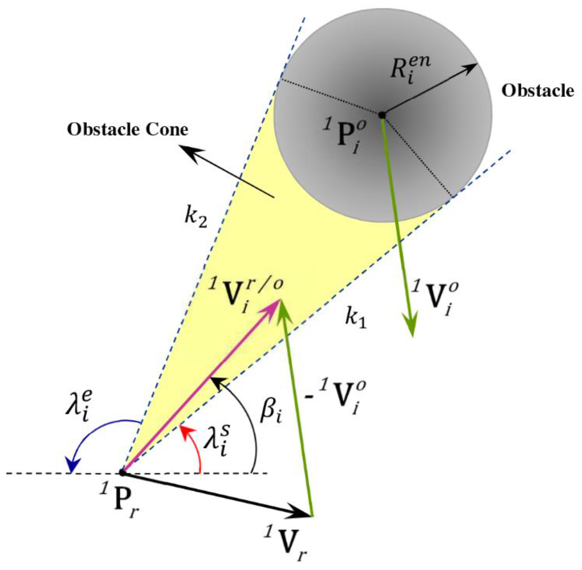
The collision cone is also defined as the planar conical region encircled by two tangent lines
and
as depicted in
Figure 2. These tangent lines are specified by their angles
and
with respect to the
x axis of frame {1}. These angles could be determined in each time
based on the enlarged obstacle radius and the position vectors of the robot and obstacle in frame {1}.
The angle of the relative velocity vector
with respect to
x axis of frame {1} is also determined as follows.
where
and
are unit vectors along x and y axes of frame {1} respectively. By defining the collision cone and relative velocity for each obstacle in time
, the collision avoidance criterion in each time instant is simply to prevent the robot from moving with the relative velocity vector inside the obstacle cone (
Figure 2). The VO set associated with
ith obstacle at time
is defined as follows.
It is obvious that the signs and values of angles
,
and
should be properly specified in different quadrants such that the comparison in Equation (36) is meaningful. Using Equation (36), the total VO set in each time instant could be defined as follows.
where
is the operator of union of sets. In addition, the total set of robot’s relative velocity vectors with respect to active obstacles in each time instant is also defined as follows.
Therefore, the collision avoidance criterion in each time
could be written in the following form.
where
is the operator of subscribe of sets and
denotes an empty set. The criterion in Equation (39) is indeed a set of constraints on the robot’s velocity vector that should be satisfied in each time step to prevent the robot from collision with obstacles. These constraints are used to specify the collision free trajectory online as a part of control system.
3.2. Model Predictive Controller
MPC is a control technique in which the control input signals are calculated based on the anticipated states of the system on a specified prediction horizon and solving online the resulting open loop optimal control problem (OCP). This construction provides a context to consider complicated constraints of the system online during the control process. Therefore, considering the collision avoidance criterion formulated in the previous section, a NMPC system is designed to move the robot towards the target position and orientation among obstacles.
To design a NMPC for discretized mathematical model of the OMR in Equation (30), the following cost function is defined.
where
is a positive definite stage cost,
is a positive definite terminal cost,
is the prediction horizon,
is the desired state,
is a sequence of
input vectors
and
. Therefore, the position and orientation of the OMR could be controlled by solving the following optimal control problem (
).
where
and
are state constraints set at time
and terminal state constraints set respectively. These sets could be determined based on the available physical constraints and collision avoidance criterion from Equation (39).
The constraints in Equation (41) are related to the robot’s mathematical model and state constraints imposed to guarantee the stability and collision avoidance in the workspace. Constraint 1 guarantees that the predicted states satisfy the robot state space model. Constraint 2 is a set of state constraints imposed to avoid collision with obstacles and defined workspace borders. Constraints 3 and 5 are associated with the initial values of states and inputs, and Constraint 4 is a terminal constraint determined in detail through stability analysis in the next section.
By solving
in each time instant
, a set of
optimal control inputs sequence is obtained as follows:
The feedback control law is defined as the first element of this optimal inputs sequence as follows, and the remaining optimal input vectors are used to form an initial guess to solve
at the next step.
Therefore, the closed loop system could be written using the feedback law in the following form:
The state constraints set
at each time
are composed of some constraints on the robot’s position and velocity and should be determined based on the physical restrictions of environment, obstacle’s positions and obstacle’s velocities. The constraints on position are indeed associated with the boundaries of the robot workspace which in turn are functions of the robot’s position at each time
. Mathematically:
where
is a closed region in frame {1} defined as:
where
,
,
and
are differentiable functions of the robot’s position vector. It is obvious that for a rectangular workspace with boundaries parallel to the axes of frame {1}, these functions are simplified to constant values. To specify the state constraints associated with the collision avoidance criterion, suppose that system’s state at time
is
and the locations and velocities of the active obstacles are calculated using robot’s sensors. The locations of the active obstacles during the prediction horizon are calculated as follows.
Using Equation (47), angles
,
and
are calculated at time
(Equations (34) and (35)) and the total velocity obstacles set could also be determined at each time using Equation (37). Therefore, the state constraints originated from collision avoidance criterion in Equation (39) is as follows.
Finally, the state constraints set could be defined in the following form.
This constraints set is indeed a set of nonlinear constraints on robot’s position and velocity vector during the prediction horizon, where is the number of active obstacles at time . These constraints guarantee that the robot remain inside the defined workspace during its motion and avoid collision with obstacles.
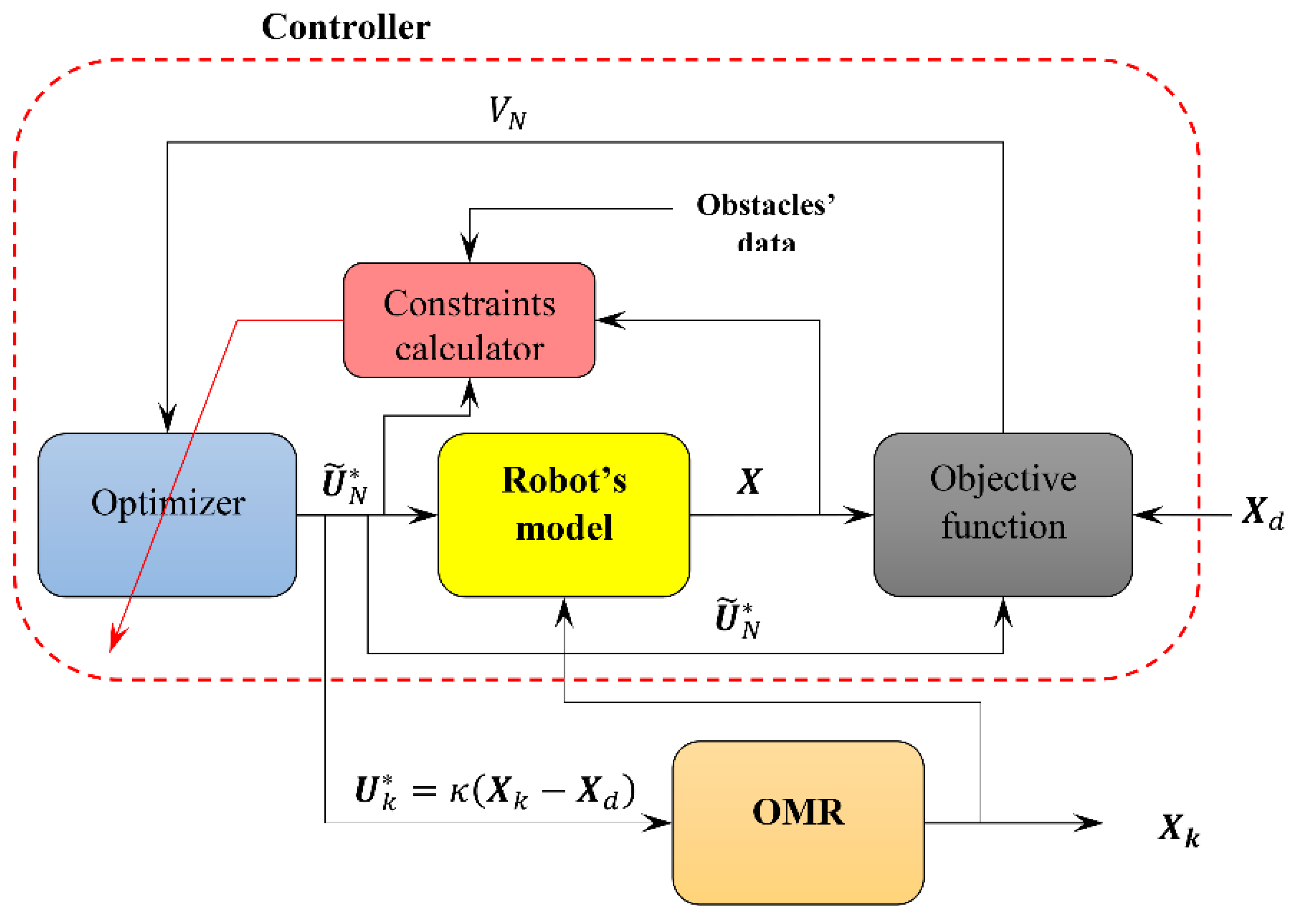
The structure of the designed control system and obstacle avoidance strategy is demonstrated in the following diagram.
Figure 3 illustrates how the optimization problem and constraints are defined in each time step and the first element of the optimal control sequence is exerted to the real robot.
3.3. Stability and Performance Analysis
The parameters and functions used to design the feedback control system in Equation (43) should be specified in which the convergence of the state variables to desired values and the acceptable performance of the obstacle avoidance strategy are guaranteed. Since the feedback control input is calculated based on the position and velocity of active obstacles, it is also assumed that the position and velocity of obstacles at time
are such that it is possible for the robot to remain inside the workspace boundaries (constraints in Equation (45)) and move towards the target position in
without collision. The first part of this assumption could be written mathematically as follows:
The second part of the assumption is associated with the possibility of moving towards the desired position without collision with obstacle and could be written mathematically as follows.
Condition in Equation (51) means that at each time
, the robot may stop at its position or move in opposite direction of desired position to avoid collision with obstacles, but it can eventually moves towards the goal at time
that the position of obstacles change. Owing to the robot capability for omnidirectional locomotion, satisfaction of (51) is guaranteed for bounded speed of obstacles, existence of a route toward the target after the time
and proper choice of control system parameters. Considering (50) and (51), the stage and terminal cost functions
and
are selected as functions of
in the following forms:
where
,
and
are diagonal matrixes defined as follows:
where
is an identity matrix and
,
and
are non-negative values. These values should be determined such that the closed loop system in Equation (44) is stable. It is clear that terminal cost
is defined as a function of state errors such that assumption in Equation (51) could be satisfied by moving the robot toward the goal. Now, suppose that
and
, omnidirectional capability of the robot implies that condition in Equations (50) and (51) are satisfied for
. Therefore,
is a control invariant set and:
where
. Considering that
(assumption (51)),
if the following is held.
Since
as robot moves towards the desired state
, for a large value of
,
is a control Lyapunov function (CLF) on
where
is a small neighborhood of the desired state. Using a sufficiently large value for
,
is sufficiently small and cost function
monotonically decreases during the robot’s motion [
37]. Therefore, the robot’s state variables converge to small vicinity of the desired state (
) as
.
If , the state constraints (49) guarantees that the robot moves without collision with obstacles. Therefore, if assumption in Equation (51) is held, the robot either moves among the obstacles toward the goal or the cost function in Equation (40) may have a local optima in opposite direction of the goal, but after some time () that obstacles move and the related velocity constraints removed, the robot can continue its motion towards the target position according to the above analysis.
Therefore, the above analysis shows that if the layout and velocity of obstacles satisfy the conditions in Equations (50) and (51) by proper choice of control system parameters, the designed control system moves the robot on collision free trajectory and stabilizes it in the desired configuration.
3.4. Control System Parameters Setup
The parameters of the control system should be specified in such a way that satisfaction of Equations (50) and (51) convergence of the state errors to zero and the acceptable performance of the collision avoidance strategy are guaranteed. As analyzed mathematically in Equations (52)–(55), parameters and affect the stability of the control system and convergence of errors to zero in the vicinity of the target position. Parameter is added in the cost function in Equation (40) to guarantee that the control inputs tend to zero and the robot completely stops in the desired configuration. Indeed, its value is important merely when the robot is in the neighborhood of the desired state and the state errors are very small. Therefore, the value of could be simply selected as . In addition, based on Equation (55), should be a large positive number to guarantee stability and convergence of the state errors to a small vicinity of the desired state.
Parameter
should be determined such that if the robot and an obstacle move toward each other at their maximum speeds, the robot is far enough away from the obstacle to avoid collision when the obstacle is detected by the robot’s sensors for the first time. The maneuver that the robot could perform in such situation is to reduce its speed to zero with maximum acceleration and then move in opposite direction with maximum acceleration to reach the maximum allowable speed of the obstacles. Therefore, parameter
should be greater than the distance that the robot and the obstacle move toward each other during this maneuver’s time (
). More precisely:
where
is the maximum allowable speed of obstacles and
denotes the distance that the robot travels before stop. Integer
in Equation (56) is indeed a safety factor and its value could be specified considering the maximum real sensors rang. While the smaller values of
and
leads to ignore the effects of far obstacles and may increase the maneuverability of the robot, the larger value of
may increase the safety of the robot maneuvers. However, using the larger value of
imposes more restrictions on the robot motion and could reduce the maneuverability of the robot in some circumstances.
Parameter is the radius of a safe region around the robot introduced to guarantee the safety of the robot motion. While state constraints in Equation (49) guarantee that the robot doesn’t collide with any obstacles at each discrete time and state ( and ), the robot’s motion is not restricted by these constraints during each sampling interval (between the times and ) and the robot may collide with close obstacles during these times. Since due to the impact of constraints in Equation (49) the distance of the robot from all active obstacles is greater than at each , the value of should be selected as the maximum distance that the robot could travel during each sampling period which is equal to . In this equation, denotes the maximum robot’s speed achieved after some time that the robot moves on straight line with maximum equal motor torques ().
Parameters
to
also affect the performance of the control system and collision avoidance algorithm. These parameters are weights coefficients for state variable errors that define the priority of each state to be converged to its desired value. Consequently, since the value of the orientation angle
and the linear and angular velocity of the robot should be controlled merely at the desired position and are not important during the robot’s motion, their associated weights are defined as follows:
where
is a constant final weights value,
and
are radius of two small circular region around the desired position,
denotes target position and
is a scalar function that should be continuous and two time differentiable at
and
. The geometrical interpretation of Equation (57) is illustrated in
Figure 4 in which the weight of position error is constant value
and the weights of other state variables increase from their initial value 0 to their final value
when the robot enters into a small neighborhood of the desired position.
It is obvious that the length of prediction horizon () could also have influence on the performance of the designed controller and collision avoidance algorithm. Since increasing the length of prediction horizon increases the computational time and cost significantly, the prediction horizon should be selected as the smallest value that leads to acceptable performance of the control system. Therefore, this value could be specified through trial and error and by evaluating the performance of the control system for different small values of .
4. Simulation Results and Discussion
To evaluate the effectiveness of the designed controller and collision avoidance algorithm two simulation experiments are conducted using MATLAB software. In these simulations, the robot moves from its initial position and orientation among the obstacles and stops at the desired state using the designed control system. The simulation is performed using the values
,
,
,
,
,
and
for the robot geometrical and physical parameters and following values for masses and moment of inertia matrixes of the robot parts.
The control input vector could be calculated by solving optimal control problem in Equation (41) in each time step. To simplify the optimization problem and to relax the constraints related to the mathematical model of the robot, recursive discretization method [
38] is used to introduce the state space model in the cost function and to reduce the numbers of nonlinear constraints. In recursive discretization method, each future state vector is calculated recursively using the previous state vector and the associated control input, and the value of the cost function is determined using the calculated states and the inputs. To solve the resulting constrained optimization problem, sequential quadratic programming (SQP) method is used here. This method is provided by MATLAB optimization toolbox (fmincon function) and it is used to solve the optimization problem in Equation (41) in each step. The control system parameters are also selected based on (55) to (57) and other criteria discussed in the previous section as
,
,
,
,
,
,
and
. Furthermore, function
could be determined as a fifth-order polynomial based on six constraints
and
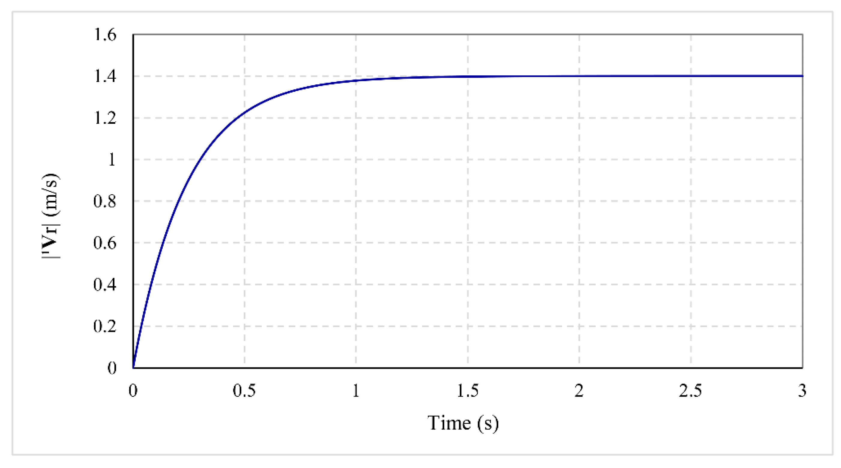
. To calculate the maximum achievable speed of the robot
, differential equations of motion of the robot in Equation (29) are solved for maximum allowable motors’ torque (
) and
. As demonstrated in
Figure 5, the robot’s speed has an upper bound at (
), due to the effects of viscous friction between the wheels and shafts. Therefore, the radius of the safe region is determined as
.
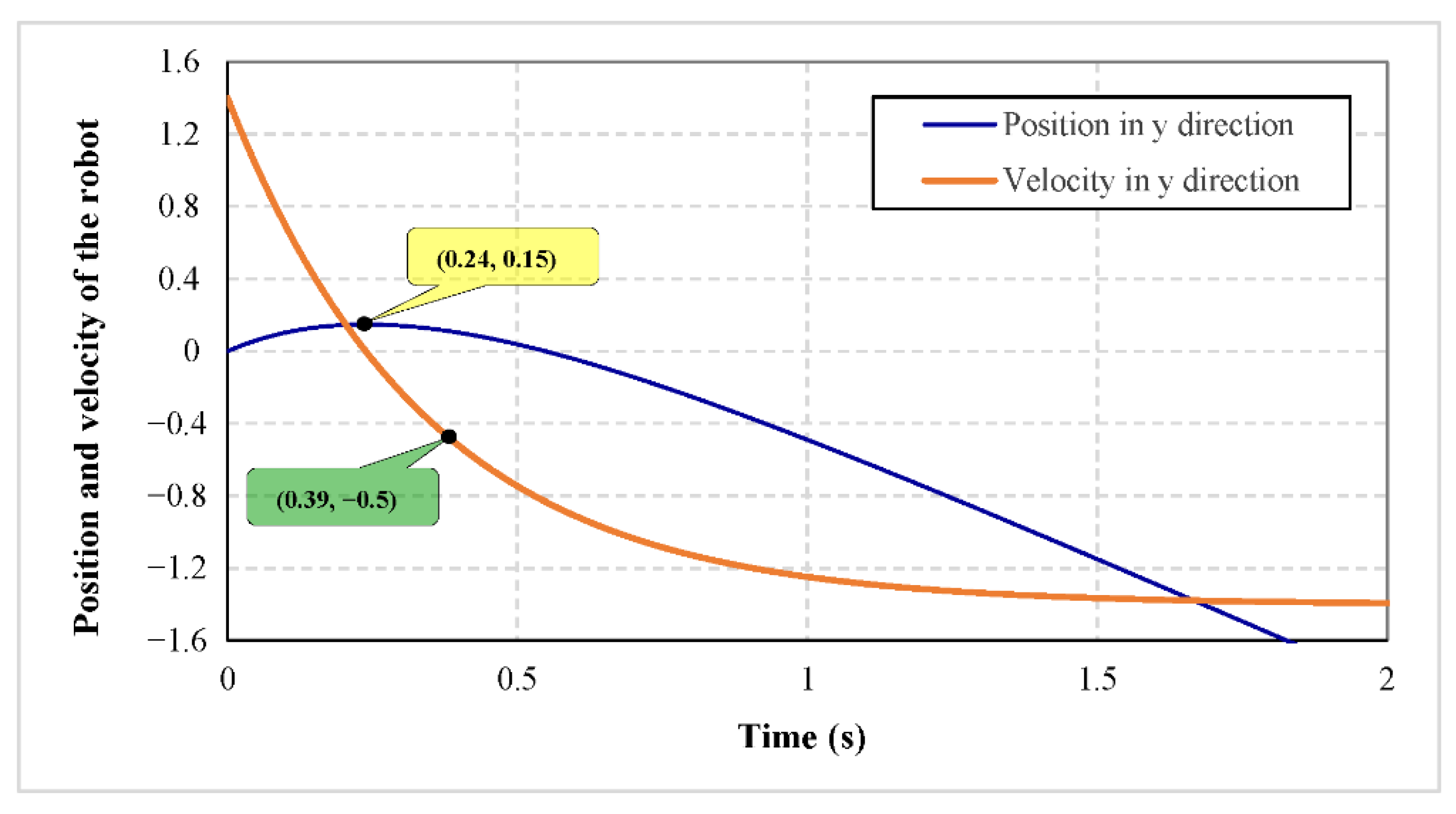
To calculate the values of parameters
and
, the robot motion is simulated in a decelerating maneuver described in
Section 3.4. Since
is defined as the maximum distance that the robot travels to reduce its speed from
to zero, the decelerating maneuver in lateral motion is considered in which the robot moves with minimum acceleration. Therefore, the differential equations of motion are solved for
and initial state
which is related to decelerating lateral motion of the robot. The variations of the position and velocity of the robot are shown in
Figure 6. Suppose that the maximum allowable speed of obstacles is
, the value of
is the robot’s position when its velocity reduces to zero, and the value of
is the time needed for the robot to reach to the maximum velocity of the obstacles in opposite direction (
).
The parameters
and
could be calculated from
Figure 6 and according to their definition in
Section 3.4 as
and
. Therefore, using Equation (56),
, and considering
and
, the performance of the control system is assessed in two following examples.
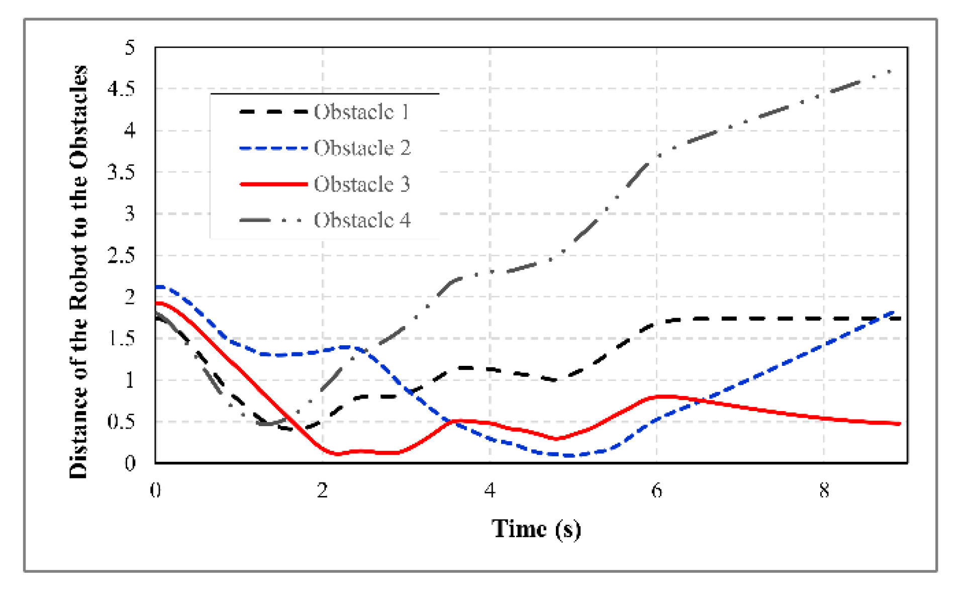
Example 1. The robot starts its motion from initial configurationto the desired stateinside a rectangular region. The robot’s workspace is defined as follows and the initial positions, velocities and radiuses of obstacles are also specified as shown in Table 1. The position and orientation errors of the robot are demonstrated in
Figure 7. It is clear that the position and orientation errors converge to zero and the robot is well stabilized in the desired position and orientation using feedback control law in Equation (43). To evaluate the performance of the designed control system in planning the robot’s trajectory and avoiding collision with obstacles the distances between the robot and obstacles (
) during the robot’s motion are illustrated in
Figure 8. The figure shows that the robot preserves the safe distance with all the obstacles in the period of its motion. It is also to be noted that since the proposed collision avoidance strategy is formulated to be combined with discrete NMPC, the distances of the robot from the obstacles are not necessarily larger than
during the robot’s motion. Indeed, using velocity constraints in Equation (48), the robot does not collide with any obstacle, if the velocity vector of the robot remains outside of the velocity obstacle set for all
. Since the robot velocity is not constant, radius
is added to the radius of obstacles to ensure collision with any obstacles not occurs during each sampling interval. This is why the value of
is determined as the maximum distance that the robot could travel during each sampling interval (
).
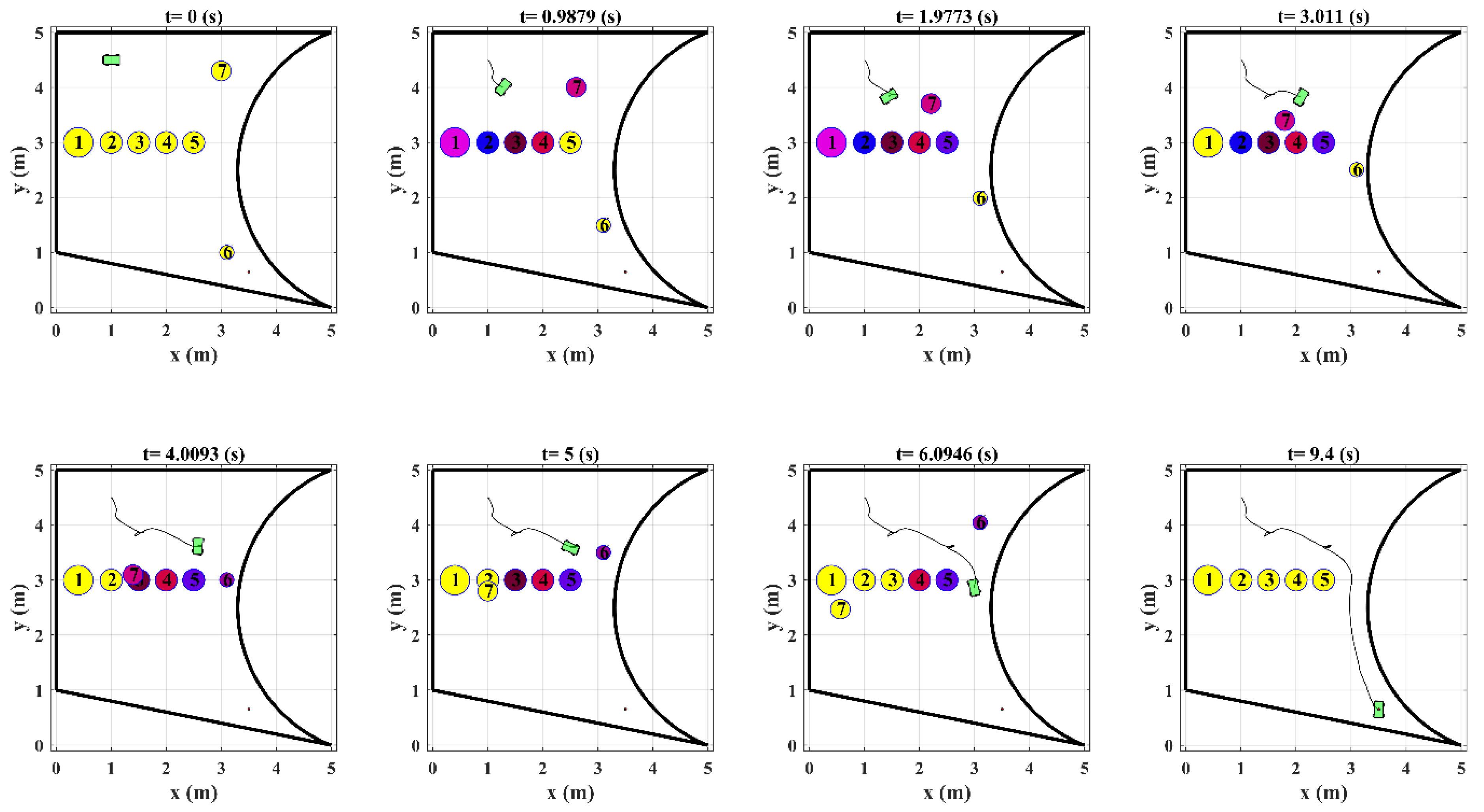
Figure 9 shows the snapshot of the robot trajectory in the presence of obstacles in which the inactive obstacles are shown by yellow color and the workspace boundaries are demonstrated by black lines. The figure shows that the arrangement and motion of the obstacles are such that the conditions in Equations (50) and (51) are satisfied and there exist a trajectory in each time step that the robot could become much closer to the target position.
Example 2. The robot’s initial configuration and the desired state are selected asandrespectively. The robot’s workspace is a region encircled by four following differentiable functions and could be defined mathematically using (46).
The initial position, velocity and radius of obstacles are selected according to
Table 2.
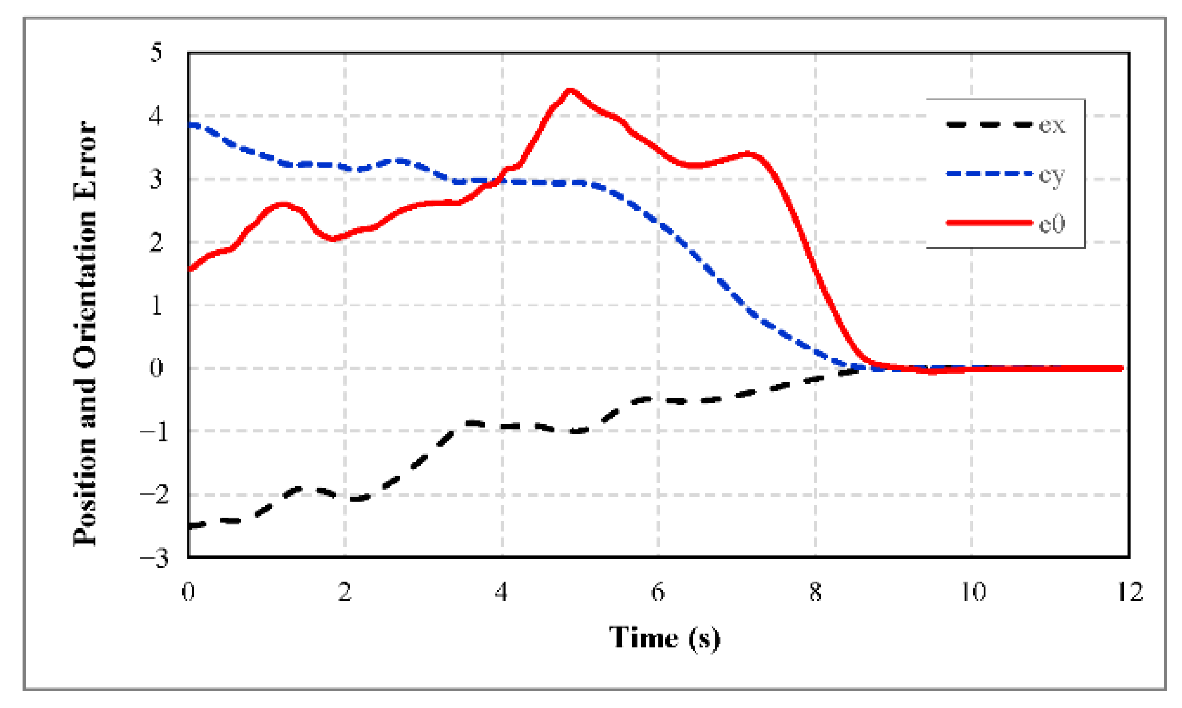
Figure 10,
Figure 11 and
Figure 12 show the simulation results of this example using the above values for the robot and control system parameters. It is clear from
Figure 10 that the position and orientation errors of the robot converge to a sufficiently small vicinity of zero as it is explained in
Section 3.3.
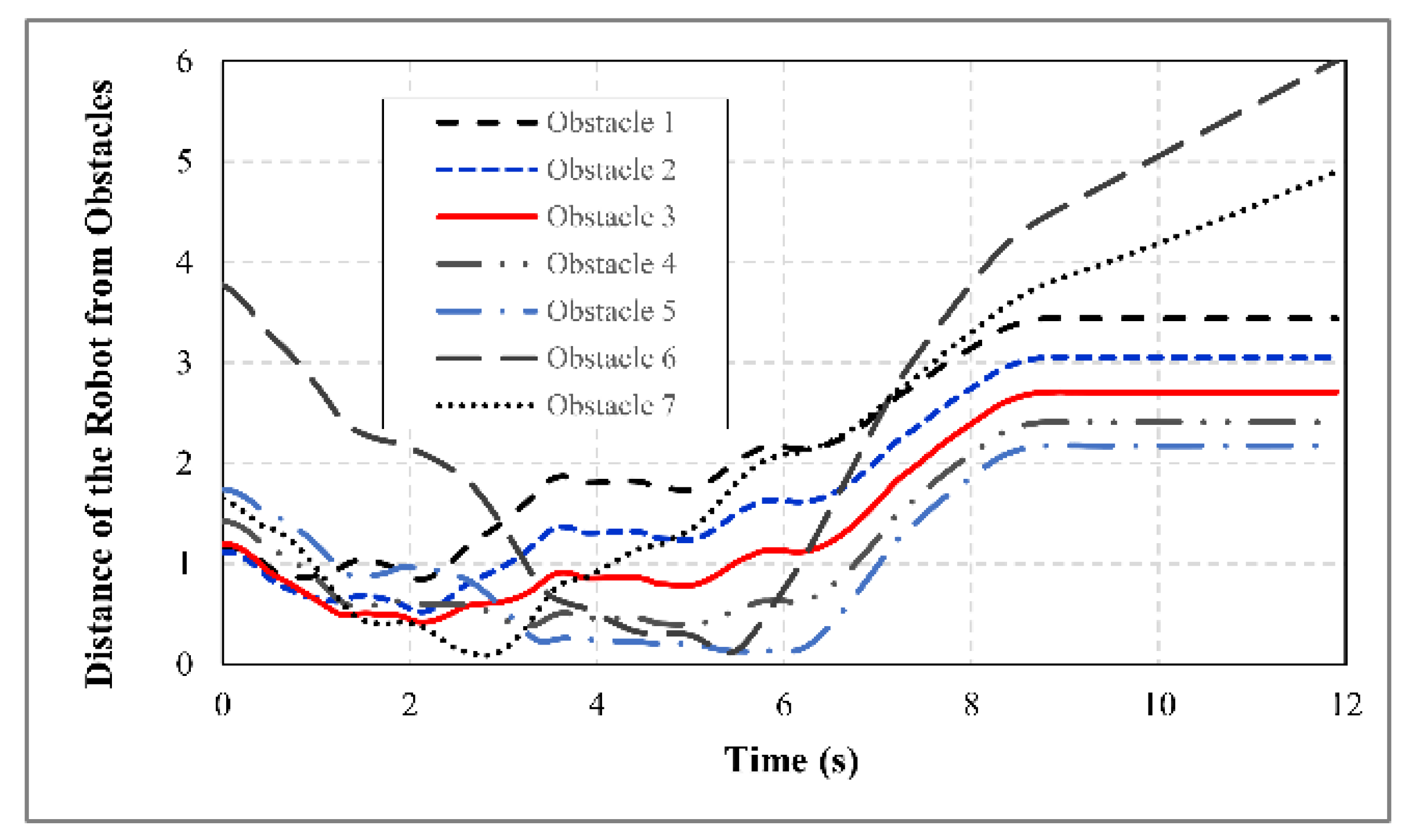
The distance of the robot from each obstacle during the robot motion is demonstrated in
Figure 11, which shows the effectiveness of the developed control strategy in protecting the robot from collision with obstacles.
As illustrated in
Figure 12, the snapshot of the robot trajectory shows that the robot remains inside the defined workspace during its motion and does not violate the related position constraints.
Figure 12 demonstrates that the region between obstacle 5 and righter border of the workspace is the only safe region which the robot can move towards the target without collision with any obstacles. However, since this region is blocked by obstacle 6, the control system stops the robot in a fragment of its motion and waits for the path to be opened for the next robot movements. This maneuver is an example of situations describe by assumption in Equation (51) and shows the effectiveness of the motion planning algorithm in such complicated arrangement of obstacles.
In addition, the arrangement and velocity of obstacles in some step times may be such that the cost function has a local minima point different with the desired state. In these situations, the velocity constraints in Equation (48) push the robot to reach the local minima point. However, since terminal cost function is selected to be a CLF, the robot continues its motion towards the goal after that the obstacles move away and the minimum point of is changed.
Figure 13 and
Figure 14 demonstrate the variation of the optimal value of the cost function
(Equation (40)) in Examples 1 and 2 obtained by solving the nonlinear constrained optimization problem in Equation (41) in each time step. It is obvious that the cost functions decrease in both cases to reach their global minima at zero, which is associated with the stabilization of the robot in desired position and orientation. However, the optimal value functions have some optimums and there are some points that the optimal value of the cost functions increases temporarily. These optimums are in fact the local minimums of the cost function in Equation (40) considering the position and velocity constraints in Equation (49) defined based on the workspace borders and collision avoidance criterion at the corresponding times. As explained mathematically in
Section 3.3 by conditions in Equations (50) and (51), these local minima points are associated with the instants that the control system has to move the robot in opposite direction of the target position to ensure that the position and velocity constraints are not violated by the robot motion.
It follows from the analyses presented in
Section 3.4 that two parameters
and
can have major effects on the shape of the robot’s trajectory before it reaches the vicinity of the target position. Parameter
affects the maximum distance that the robot could travel in each sampling period and has a direct relationship with the safe region
. On the other hand, parameter
affects the value of
which in turn has a main effect on the number of detected and active obstacles in each time instant. Therefore, increasing or decreasing the values of these parameters could change the route that the control system selects in each sampling time to move the robot toward the goal and prevent collision with obstacles.
To evaluate the effects of these parameters on the performance of the design control system, solving Examples 1 and 2 are repeated using different values of
and
.
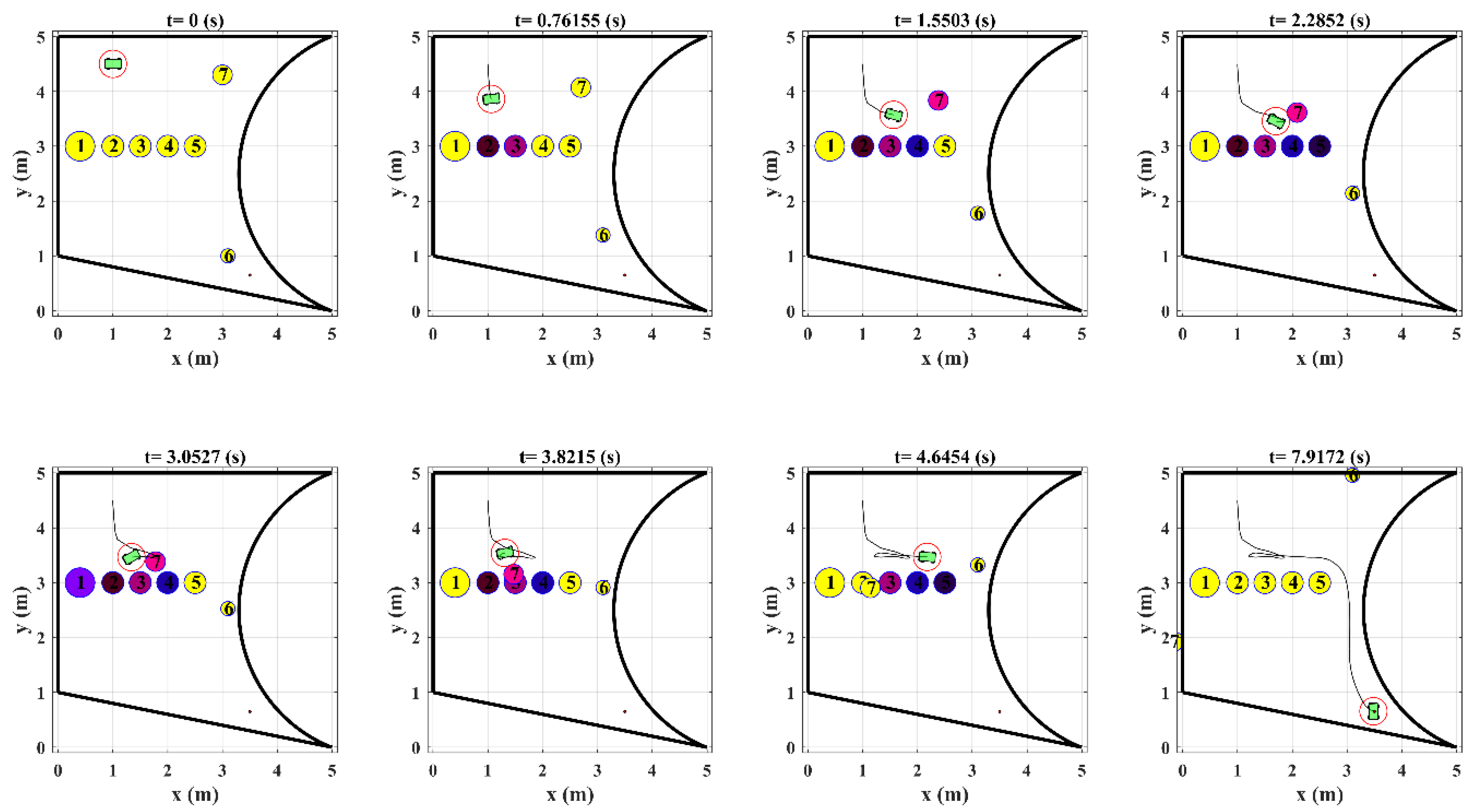
Figure 15 illustrates the snapshot of the robot’s motion in Example 1 for
and
.
By increasing the value of , the far obstacles are also detected, which has significant influences on the geometry of robot path toward the target position. Although increasing the value of in Example 1 helps the control system to consider the effects of far obstacles and find a safer path toward the goal, this may impose more restriction on the robot motion and reduce the robot maneuverability in more crowded environments.
The simulation results of Example 2 for
and
is shown in
Figure 16. By reducing the value of
, the radius of the safe region decreases to
and the robot could move closer to obstacles. Furthermore, using the smaller value for
leads to neglect the effects of far obstacles and reduce the number of velocity constraints on the robot motion. Compared to the simulation results illustrated in
Figure 12,
Figure 16 shows that the only effects of closer obstacles are considered. Therefore, the robot gets closer to obstacles before it changes its direction to avoid collision.
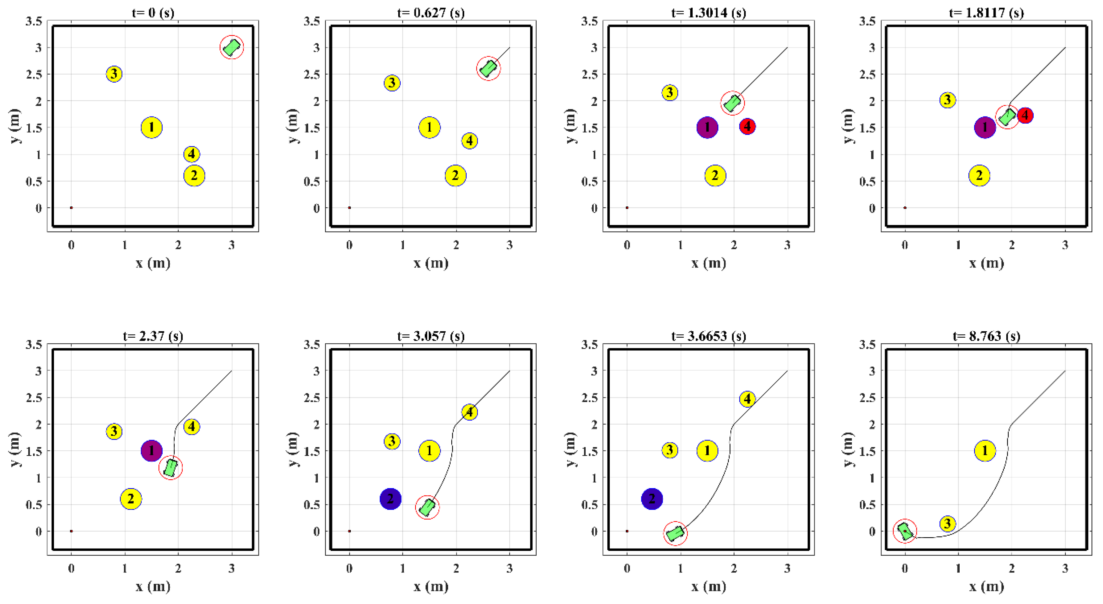
Figure 17 shows the simulation results of Example 1 for
and
. Using this value for
, the radius of the safe region is
and therefore the robot could move in narrow passages and much closer to workspace borders. In addition, using the minimum allowable value for
, the robot travels longer distance on straight line trajectory than shown in
Figure 9, until it detects the obstacle 1 for the first time. In comparison to
Figure 9 and
Figure 15,
Figure 17 shows that by using the smaller value for
and
, the control system chooses the narrow space between the obstacles 1 and 4 for the robot’s motion and the robot travel on a shorter path to reach the goal.
The effects of the parameters
and
on the shape of the robot trajectory in the above simulations results are summarized in
Table 3. These effects are evaluated and compared based on two quantitative and two qualitative metrics. The quantitative metrics are the length of trajectory and the total time required for the robot to reach to the target position. On the other hand, the qualitative metrics are using safer spaces for the robot’s motion and the ability of moving in narrow spaces between obstacles. While the safer spaces are defined as part of workspace with low density of obstacles, the ability of moving in narrow spaces could be regarded as the capability of selecting narrower spaces between the obstacles to move the robot on faster trajectory or on closer to straight line trajectory.
It is clear from
Table 3 that by increasing the value of
the number of detected obstacles increases and by considering the effects of far obstacles, the control system could detect empty spaces in the workspace for the robot’s motion. On the other hand, by decreasing the value of
, the control system neglects the effects of far obstacles and consequently tries to move the robot faster toward the target. Furthermore, by decreasing the value of
, the value of
also decreases and the control system could select narrow spaces between obstacles to move the robot toward the goal. As demonstrated by the data presented in
Table 3, the fastest trajectory is obtained using the minimum value of
and
. These values are related to simulation results presented in
Figure 17 in which the control system not only neglect the effects of far obstacles in each sampling interval, but also use the narrow space between obstacles 1 and 4 for the robot motion. It is also clear from
Table 3 that the safer trajectories in Examples 1 and 2 are obtained using the larger value of
. Nevertheless, increasing the value of
leads to increase the number of imposed velocity constraints on the robot’s motion and may have negative effects in crowded environments. Therefore, the appropriate values of
and
could be selected based on the general layout of obstacles and other important factors in each circumstances.
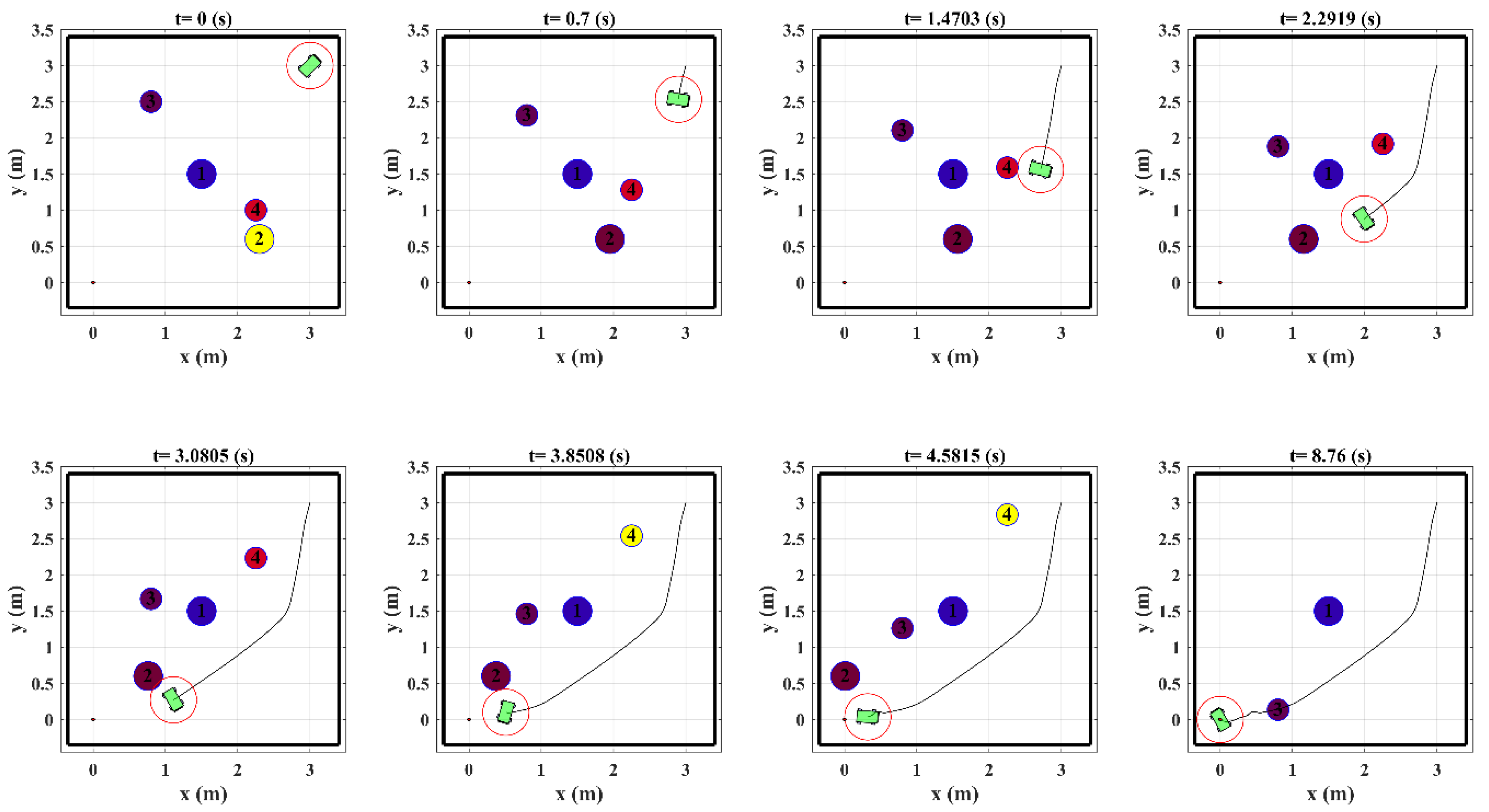
To assess the performance of the proposed control system and obstacle avoidance strategy in comparison with other methods, the robot‘s motion between fixed and moving obstacles is simulated for the Example 3 presented in [
26]. The velocity and initial position of the obstacles are specified based on the data provided in [
26]. In addition, the maximum allowable motors’ torque and the value of the viscous friction coefficient are specified as
and
in such a way that the maximum acceleration and velocity of the robot are equal to the values reported in [
26] (
and
). In addition, considering
, the value of parameters
,
and
are calculated as 0.062 m, 1.57 s and 0.1374 m, respectively. Since the maximum obstacle‘s speed in this example was
, the minimum value of
is calculated from Equation (56) as
. Using the initial and desired configuration of the robot, similar to [
26], as
and
, the snapshot of the robot’s motion among the obstacles is obtained by the proposed method in this paper and depicted in
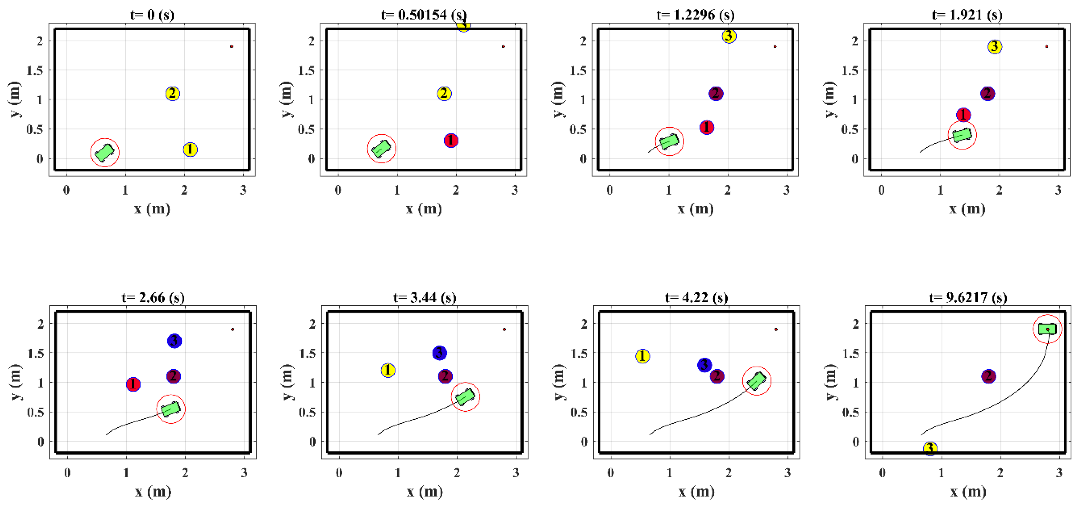
Figure 18.
Figure 18 shows that the robot successfully reaches the target configuration without collision with obstacles. Compared to the results of simulation provided in [
26], the robot selects a safer trajectory toward the goal without facing the obstacle 3. This is because the NMPC system that choses the fastest route toward the target after the robot turns right to escape from the obstacle 1. The simulation results presented in [
26] demonstrate that the robot restricted to move on straight line trajectory between the start and the target position, and changed its direction once the obstacle detected. However, such a trajectory is not necessarily the best and the safest one. In addition, it may be even impossible for the robot to move on the trajectory calculated by this algorithm in complicated situations such as Example 2 that the robot should stop in some positions and wait for the route to be opened.


