1. Introduction
Robots have been widely utilized for industrial tasks including assembly, welding, painting, packaging, and labeling. In many cases they are controlled to track a given trajectory by external motion command interfaces, which are available for many industrial robot controllers, including the MotoPlus of Yaskawa Motoman, low-level interface (LLI) for Stäubli, robot sensor interface (RSI) of Kuka, and externally guided motion (EGM) of ABB. Although high-precision industrial robots have been well established for decades in manufacturing and fabrication applications that require precise motion control, such as aerospace assembly, laser scanning, and operation in crowded and unstructured environments, it still remains a challenge to track a given trajectory accurately. In general, a trade-off exists between reduction of cycle time and improvement of tracking accuracy for industrial robots.
Trajectory tracking control of robot manipulators is a well-studied problem [
1]. The typical control architecture is based on joint torque control, which is challenging to implement on industrial robots. The controller structure usually consists of a linear stabilizing feedback controller and a feedforward compensation for trajectory tracking. Asymptotically perfect tracking is achieved by adaptive control [
2], given that the robot dynamics are expressed in the linear-in-parameter form. However, accurate dynamics information for a robot is rarely available in practice. In this case, either simplified reduced-order models are identified [
3], or machine learning techniques including wavelet networks, Gaussian Processes, and fuzzy logic systems [
4] are utilized to approximate a sophisticated model for controller design. Iterative learning control (ILC) [
5,
6] relaxes the requirement of model information, but the learned representation is not transferable between different trajectories. Recently, neural network (NN)-based [
7] controller design has attracted a great deal of attention with its potential ability to generalize beyond the training set. A detailed review of neural-learning control is presented in
Section 2.
The goal of this work was to design an outer-loop feedforward controller to compensate for the inner-loop dynamics for the trajectory tracking control of an articulated industrial robot. Our approach, as illustrated in
Figure 1, combines iterative learning control with a multi-layer neural network (MNN). ILC finds the commanded robot motion corresponding to a collection of desired robot joint trajectories. These input/output trajectory pairs are then used to train the inverse dynamics of the inner control loop (with desired robot joint trajectory as the input and commanded robot motion as the output) represented as an MNN (Neural Network I, NN-I, in
Figure 1). As the inner loop may be non-minimum-phase (from time delay or non-collocated input/output map due to joint or structural flexibility), the MNN needs to be able to approximate a non-causal system to avoid instability. We used a robot dynamics simulator from a robot vendor (RobotStudio from ABB) to rapidly generate a large set of training trajectories. The simulator was also used to guide the training process and evaluate the performance of the trained MNN. When the NN feedforward control is applied to a physical robot, the tracking performance invariably degrades due to the discrepancy between simulation and reality. To narrow this reality gap, the output layer of NN-I was adjusted using a moderate amount of additional data obtained from the physical robot. This process is similar to transfer learning [
8]. Using the proposed approach, we have demonstrated significantly improved tracking performance on a physical robot ABB IRB 6640-180 using NN compensation. We have also applied the trained NNs (NN-I) to two other robot models in simulation and both show improved tracking.
Compared to state-of-the-art neural-learning controller design, the contributions of this paper are as follows.
Non-causal MNN for stable nonlinear inversion: We showed the feasibility of using an MNN to approximate the non-causal stable inverse for nonlinear non-minimum-phase robot inner-loop dynamics.
Model-free iterative learning: We demonstrated a model-free gradient-based ILC law for nearly diagonal robot inner-loop dynamics. This ILC was used to generate the training set for the MNN.
Transfer learning: We narrowed the reality gap by updating the output layer of the simulation-trained MNN using the data from the physical robot.
Demonstration: The improved performance using our approach was shown through simulation and experimental trials with a 6-degree-of-freedom (dof) nonlinear industrial robot.
Generalizability: Different robots from the same vendor exhibit similar inner-loop dynamics. We showed that the MNN trained for one robot improves the performance on other robot models from the same vendor as well.
The rest of the paper is organized as follows.
Section 2 summarizes related work on neural learning for robot trajectory tracking control and highlights our contributions.
Section 3 states the problem, followed by the methodology in
Section 4. The simulation and experimental results are presented in
Section 5. Finally,
Section 6 concludes the paper and adds some new insight.
2. Related Work
Numerous techniques have been proposed to control uncertain nonlinear dynamical systems using universal approximators such as Gaussian processes [
9] and neural networks [
10,
11,
12]. In a general framework of neural-learning control, NNs are used to either approximate the robot forward dynamics or inverse dynamics for controller design [
13], and the control problem falls within the context of either reinforcement learning [
14,
15], adaptive control [
16], or optimal control [
17]. Radial basis function (RBF) NNs, multi-layer feedforward NNs, and recurrent neural networks (RNNs) have been explored for trajectory tracking control [
18,
19,
20,
21,
22]. The concept of incorporating fuzzy logic into NN control has also grown into a popular research topic [
23,
24,
25,
26].
Radial basis function NNs are a popular choice in neural adaptive controller design since they naturally express the dynamics approximation into a linear-in-parameter form [
27]. In [
28], an adaptive control strategy in joint torque level using RBF NNs for dynamics approximation was proposed to compensate for the unknown robot dynamics and an unknown payload. However, typically, a large amount of parameters are required to approximate robot dynamics accurately by using the RBF NNs, and it is a non-trivial task to select the centers and shapes of radial basis function kernels. In addition, users usually only have access to the joint position or velocity setpoint control for many industrial robots. In [
29], a neural adaptive control technique was introduced for a trilateral teleoperation system with dual-master/single-slave manipulators. In [
30], a NN-based sliding mode adaptive controller achieved robust trajectory tracking control for robot manipulators subject to uncertainties. However, torque control was required and only simulation results were presented. An adaptive controller based on a two-layer feedforward perceptron NN was proposed in [
31,
32] for robot manipulator control. The adaptation of the unknown parameters was derived by the Lyapunov stability analysis and Taylor series expansion. However, the extension to more layers becomes more complex. Adaptive neural control methods have also been investigated for humanoid robots [
33,
34]. Other proposed control frameworks that use general function approximators for linearizing controller design can be found in [
35,
36,
37].
There have been several approaches that use NNs to approximate a system inverse for dynamical compensation [
38,
39,
40]. None of these approaches consider the possible non-causality in stable dynamical inversion. In [
41], a double-NN architecture was introduced, with one NN for the nonlinear system identification and another one learning the system inverse. However, the structure was complex and led to more parameters. It has also been shown that RNN outperforms Gaussian processes [
9] in the performance of learning robot inverse dynamics with linear time complexity, given sufficient training data [
42].
Our focus is on inner-loop dynamics compensation rather than torque-level control, which is more readily applicable to current industrial robots. The inner-loop dynamics are stable and nearly diagonal, but may be non-minimum-phase due to time delay or unstable zero dynamics. The use of an MNN for robot control in this setting is new and unique.
3. Problem Statement and Approach
Consider an
n-dof robot arm under closed-loop joint servo control with input
, typically either the joint velocity command
or the joint position command
, and the output
, the measured joint position. The inner-loop dynamics,
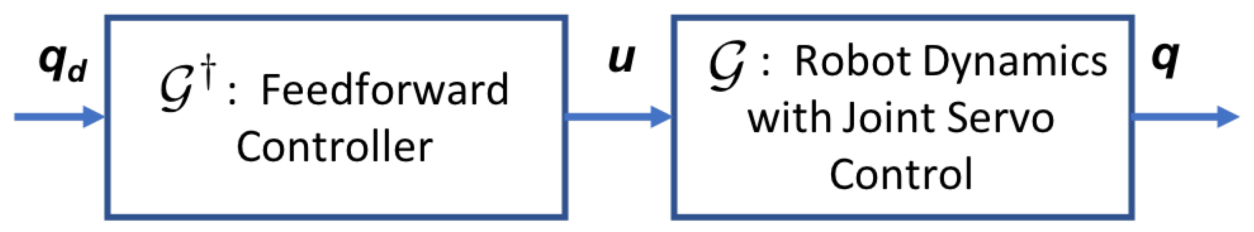
, is a sampled-data nonlinear dynamical system possibly with communication transport delay and quantization effects. Our goal is to find a feedforward compensator
(as shown in
Figure 2) such that, for a given desired joint trajectory
, the feedforward control
would result in asymptotic tracking:
, as
.
As is assumed unknown, we will use a multi-layer neural network to approximate . The plant may be non-minimum-phase (e.g., due to time delay or unstable zero dynamics from joint flexibility), so the causal inverse would be unstable. In this case, a stable inverse exists but is non-causal. Therefore, the neural network approximation of must be able to represent the possible non-causal property.
Locally, near a given configuration, is a linear system that may be represented by an auto-regressive/moving-average (ARMA) model in the sampled-data implementation. As the coefficients in the ARMA model may depend on the robot pose, a global representation of is a nonlinear ARMA (NARMA) model. Similarly, may also be represented by a stable but possibly non-causal NARMA model. In this case, a multi-layer feedforward network with a window of past and future inputs is a natural candidate to approximate . Note that since the desired trajectory is assumed to be known, future may be used in the non-causal implementation. It is also possible to directly use a recurrent neural network (RNN) to directly capture the dynamics in . A bidirectional recurrent neural network (BRNN) may be needed to capture the non-causal behavior.
We used an ABB IRB6640-180 robot as a test platform. IRB6640-180 is a robot manipulator with six revolute joints, a 180 kg load capacity and a maximum reach of 2.55 m. It has high static repeatability (0.07 mm) and path repeatability (1.06 mm) [
43]. In this paper, we assume the robot internal dynamics and delays are deterministic and repeatable, which is reasonable considering the high accuracy and repeatability of the robot. The ABB controller has an optional externally guided motion (EGM) module [
44], which provides an external interface of commanded joint angles,
, and joint angle measurements at a 4 ms rate. ABB also offers a high-fidelity dynamical simulator, RobotStudio [
45], with the same EGM feature included. We used this simulator to implement ILC and in turn generate a large amount of training data for
implemented as a multi-layer NN.
EGM sends the commanded joint angle to the low-level servo controller as a setpoint, and reads the actual joint angle vector, , measured by the encoders. Ideally, should be the identity matrix. However, because of the robot dynamics and the inner control loop, is a nonlinear dynamical system.
4. Methodology
Though may be implemented in simulation and physical experiments, finding is challenging because is difficult to characterize analytically. Our approach to the approximation of does not require the explicit knowledge of and only uses for a specific input u. The key steps include the following.
Model-free gradient descent-based iterative refinement: For a specific desired trajectory
, we approximate
by a linear time-invariant system
. The gradient descent direction
(
is the adjoint of
), may be approximated by
. As shown in [
46], this can be obtained using
for a suitably chosen
u.
Approximation of dynamical system using a feedforward neural network: The first step generates multiple trajectory pairs corresponding to . We would like to approximate by a feedfoward neural network and train the weights using from iterative refinement. To enable a feedforward net to approximate a dynamical system, we use a batch of to generate a batch of u. Furthermore, the batch is shifted with respect to u to remove the effect of transient responses.
Improvement of neural network based on physical experiments: We perform the first two steps using a dynamical simulator of (in our case, RobotStudio). When the trained NN approximation of is applied to the physical system, tracking errors may increase due to the discrepancy between the simulator and the physical robot. Instead of repeating the process all over again using the actual robot, we just retrain the output layer weights of the NN.
The rest of this section describes these steps in greater details.
4.1. Iterative Refinement
Consider a single-input/single-output (SISO) linear time-invariant system with transfer function
, input
u, and output
y. We use the underline of a signal to denote the trajectory of the signal over
for a given
T. Given a desired trajectory
, the goal is to find an optimal input trajectory
so that the
-norm of the output error,
, is minimized. Given an initial guess of the input trajectory
, we may use gradient descent to update
:
where
is the adjoint of
,
, and
. The step size
may be selected using a line search to ensure the maximum rate of descent. Let the state space parameters of a strictly proper
be
, i.e.,
. Then
. Since
A is stable,
would be unstable and
cannot be directly computed. For a stable computation of the gradient descent direction, we use the technique described in [
46,
47]. We propagate backward in time with time-reversed
to stably compute the time-reversed gradient direction. The result is then reversed in time to obtain the gradient descent direction forward in time. The key insight here is to perform the gradient generation using
instead of an analytical model of
. As a result, no explicit model information is needed in the iterative input update. The process of one iteration of gradient descent based on
is shown in Figure 2 of [
47] and described below.
- (a)
Apply to the system at a specific configuration and obtain the output and corresponding tracking error .
- (b)
Time-reverse to .
- (c)
Define the augmented input . Let with the system at the same initial configuration as in step (a).
- (d)
Compute , and reverse it in time again to obtain the gradient direction .
The above iterative refinement algorithm is easily applied to a single robot joint with
given by RobotStudio. The first guess of
is simply chosen to be the desired output trajectory
. The convergence and robustness analysis of the gradient-based ILC can be referred to in [
47]. We may also fit the response of RobotStudio using a third-order system (an underdamped second-order system cascaded with a low-pass filter) within the linear regime of the response:
Within the linear regime, may be used instead of to speed up the iteration (as RobotStudio is more time-consuming than computing a linear response).
Table 1 compares the tracking errors
in RobotStudio, with using RobotStudio or the fitted linear model to generate the gradient descent direction. As the amplitude and frequency of the desired output is still in the linear regime, both approaches work well.
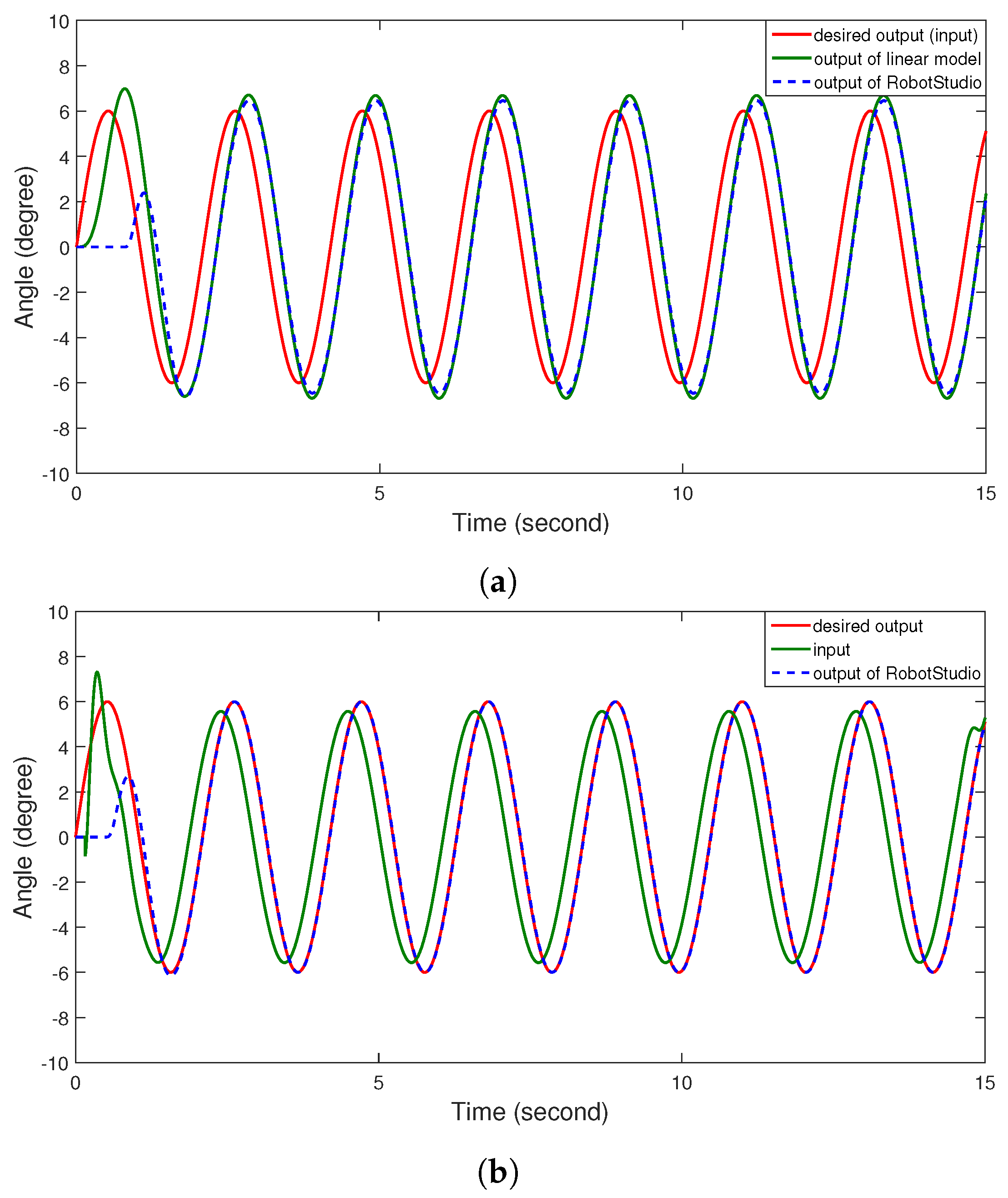
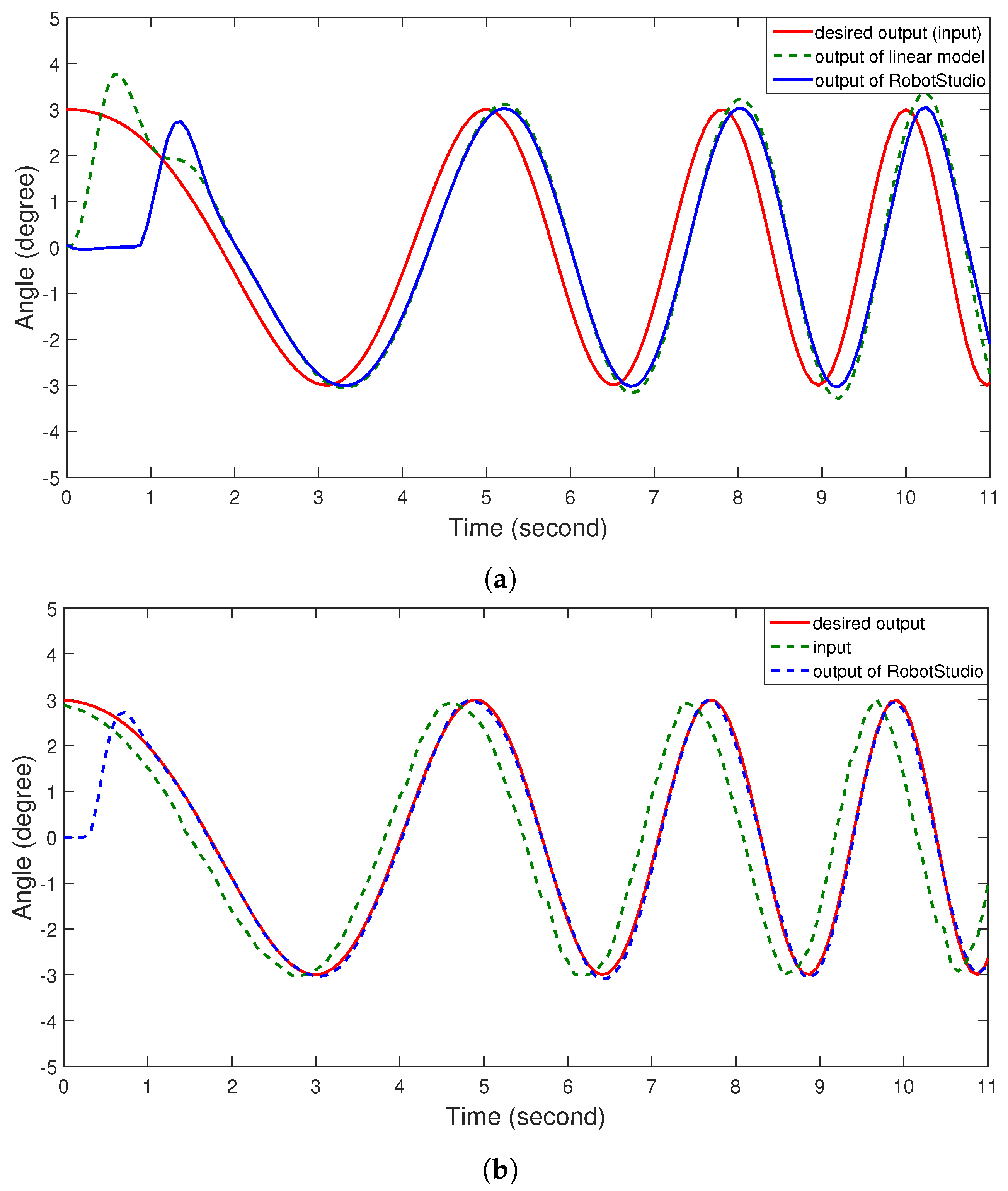
Figure 3 shows the trajectory tracking improvement of a sinusoidal trajectory.
Figure 3a reports the uncompensated case (i.e.,
). RobotStudio output indicates an initial dead time and transient, but matches well with the linear response afterwards. Because of the RobotStudio dynamics, there is a significant tracking error in both amplitude and phase.
Figure 3b shows the input
and output
after 8 iterations. After the initial transient,
and
are almost indistinguishable. The input
has amplitude reduction and phase lead compared to
(also
) to compensate for the amplitude gain and phase lag of RobotStudio for the input
.
The inner-loop control for industrial robots typically tightly regulates each joint, and the system is almost diagonal as seen from the outer loop. Therefore, the single-axis algorithm may be directly extended to the multi-axis case by using the same iterative refinement procedure applied to each axis separately.
4.2. Feedforward Neural Network
Despite the significantly improved tracking performance, iterative refinement finds
only for a local specific
. Our aim is to obtain a global approximation of
directly by learning from a set of
obtained from iterative refinement. To this end, we use multi-layer NNs to represent
. Due to the decoupled nature of
(command of joint
i only affects the motion of joint
i), we have
n separate NNs, one for each joint. We train these NNs from scratch using a large number of sample trajectories covering the robot workspace, and the corresponding required inputs are obtained by iterative refinement as described in
Section 4.1.
We hypothesize that
may be represented as a nonlinear ARMA model. We use a feedforward net to approximate this system, similar to [
48]. At a given time
t, the input of the NN is a segment of the desired joint trajectory
. The output is also chosen as a segment of
u:
. Updating a segment of the outer loop control instead of a single time sample reduces computation by avoiding frequent invocation of the NN. The choice of the future segment of
is to allow approximation of non-causal behavior needed in inverting the non-minimum phase or strictly proper
.
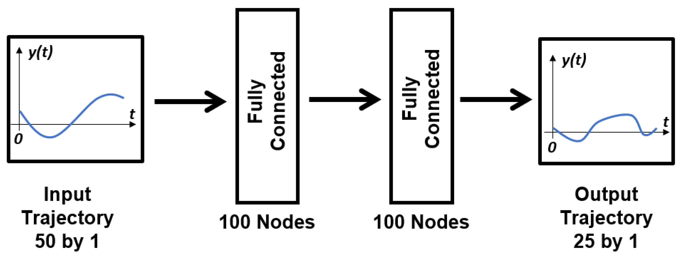
We explored the NN architectures, particularly the number of hidden layers and the number of nodes in each layer, by experiment. The selection of
T (identically, the input dimension of NNs) should guarantee that the input of NNs contains enough information for the NNs to model the dynamics, and at the same time should not be too large or it requires a lot more training data. By testing, we chose
T to correspond to 25 samples (in the case of EGM with a 4 ms sampling rate,
s). The input and output layers therefore have 50 and 25 nodes, respectively.
Table 2 lists the results of mean-squared testing error on unseen testing data with different architectures.
After testing, we selected a fully-connected network including two hidden layers, and each hidden layer contained 100 nodes, as illustrated in
Figure 4. To cover the workspace of the robot as much as possible, the robot started at a random configuration and each trajectory was composed of 3000 samples, or 12 s. A large amount of trajectories, including sinusoids, sigmoids, and trapezoids, were collected to train the NNs in
TensorFlow on a NVIDIA GeForce GTX 1050 Ti GPU card, completing in around 45 min. The main Python file ran on a desktop with an Intel Core i7-7700 CPU with 4 cores and 8 logical processors. We used a per-GPU batch size of 256, and used
norm regularization to avoid overfitting, and the rectified linear unit (ReLU) function to introduce nonlinearity for the NNs. A fixed learning rate of
was employed for the training using
AdamOptimizer. Using trajectories with different velocity and acceleration profiles, we were able to activate and collect data from both linear and nonlinear regions of EGM.
4.3. Transfer Learning
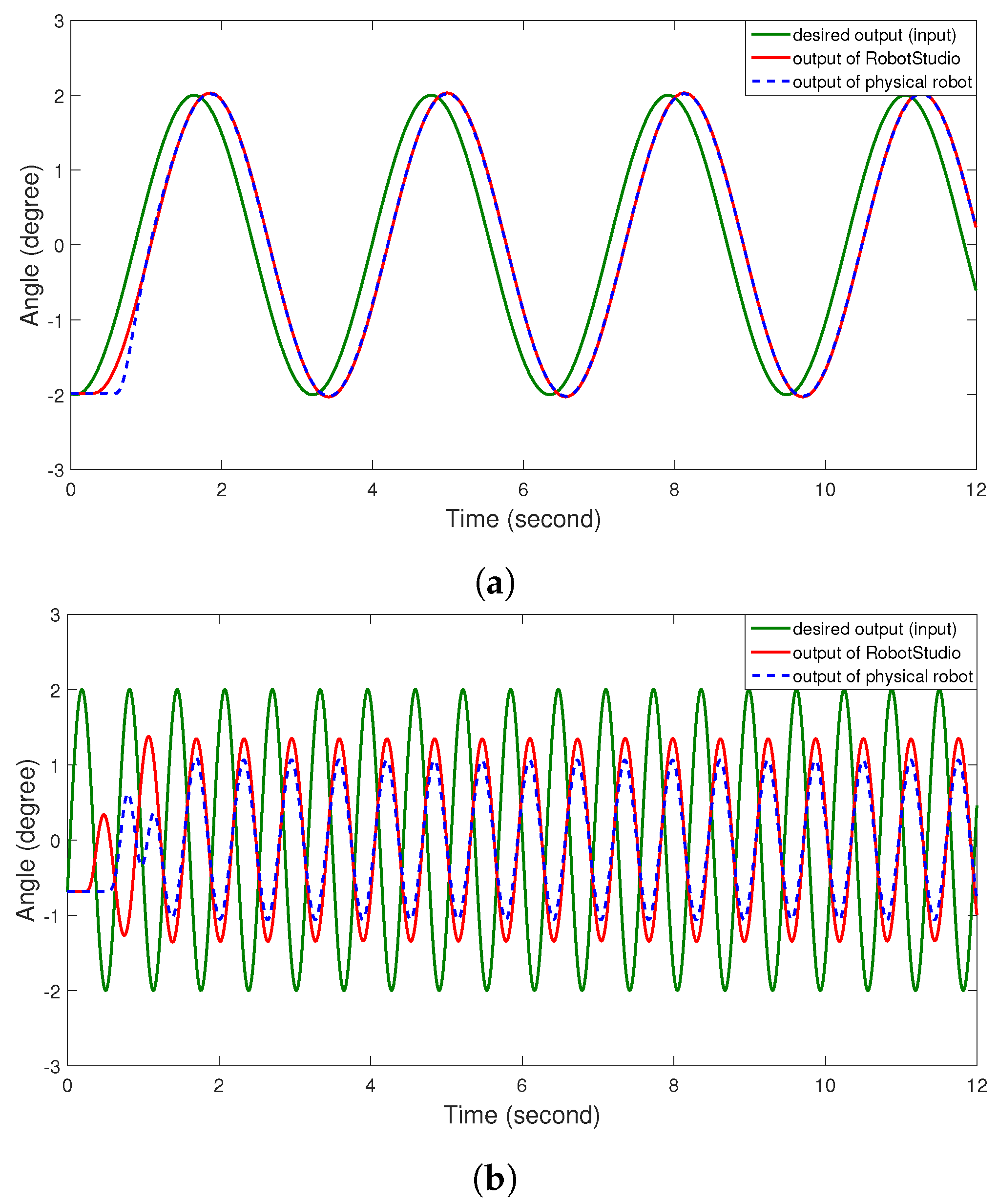
A reality gap exists between RobotStudio and the physical robot due to model inaccuracies and external physical load (such as grippers and cameras) on the physical robot. RobotStudio captures the dynamics of the physical robot very well for a trajectory with low velocity, as in
Figure 5a. However, for trajectories with large velocity and acceleration, discrepancies between RobotStudio and physical robot responses become obvious (mainly in the output magnitude) as shown in
Figure 5b.
To narrow down the reality gap between the simulator and the physical plant, we applied the iterative refinement procedure on the physical robot for 20 different trajectories and used the results to fine-tune the output layer weights of the trained NNs. The trained NNs are essentially regarded as a feature extractor. As only the amplitudes of the response showed discrepancies (as shown in
Figure 5), it was reasonable to only fine-tune the output layer weights using data from the physical robot, with the parameters of the first two layers of NNs fixed.
5. Results
5.1. RobotStudio Simulation Results on IRB6640-180
5.1.1. Single-Joint Motion Tracking
As multiple sinusoids were used in the training of the NN (with discrete angular frequencies ranging from 0.5 to 15 rad/s), we tested its generalization ability on a chirp (multi-sinusoids) that was not part of the training set (with continuous angular frequencies ranging from 0.628 to 1.884 rad/s).
Figure 6 illustrates the result for joint 1 of the simulated robot with NN compensation.
Figure 6a shows the uncompensated output with the robot output lagging behind the desired output. The nonlinear effects are denoted by the deviation of the linear model output from the RobotStudio output.
Figure 6b shows that, by compensating for the lag effect and amplitude discrepancies, the command input generated by the NN drives the output to the desired output closely after a brief initial transient.
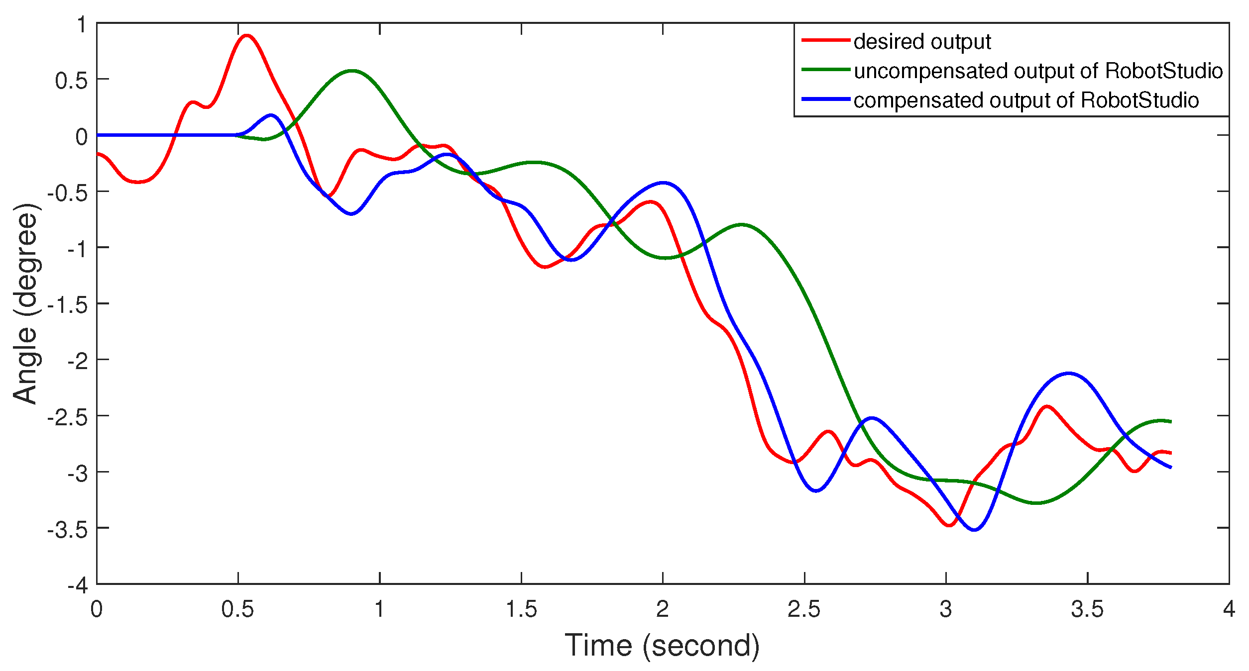
To test the generalization capability of the trained network beyond the sinusoidal trajectory,
Figure 7 shows the tracking result of a random trajectory generated from a uniform distribution for joint 1 of the simulated robot. The trained NN works for compensating for the lag effect and amplitude degradation, though not as well as for the chirp signal.
5.1.2. Multi-Joint Motion Tracking
Figure 8 compares the tracking of a 6-dimensional sinusoidal joint trajectory (
= 5 rad/s, and with different amplitudes and phases from the training data) without and with NN compensation.
Table 3 lists the corresponding tracking errors in terms of
and
norms (using error vectors at each sampling instant). The
error was calculated by ignoring the initial transient.
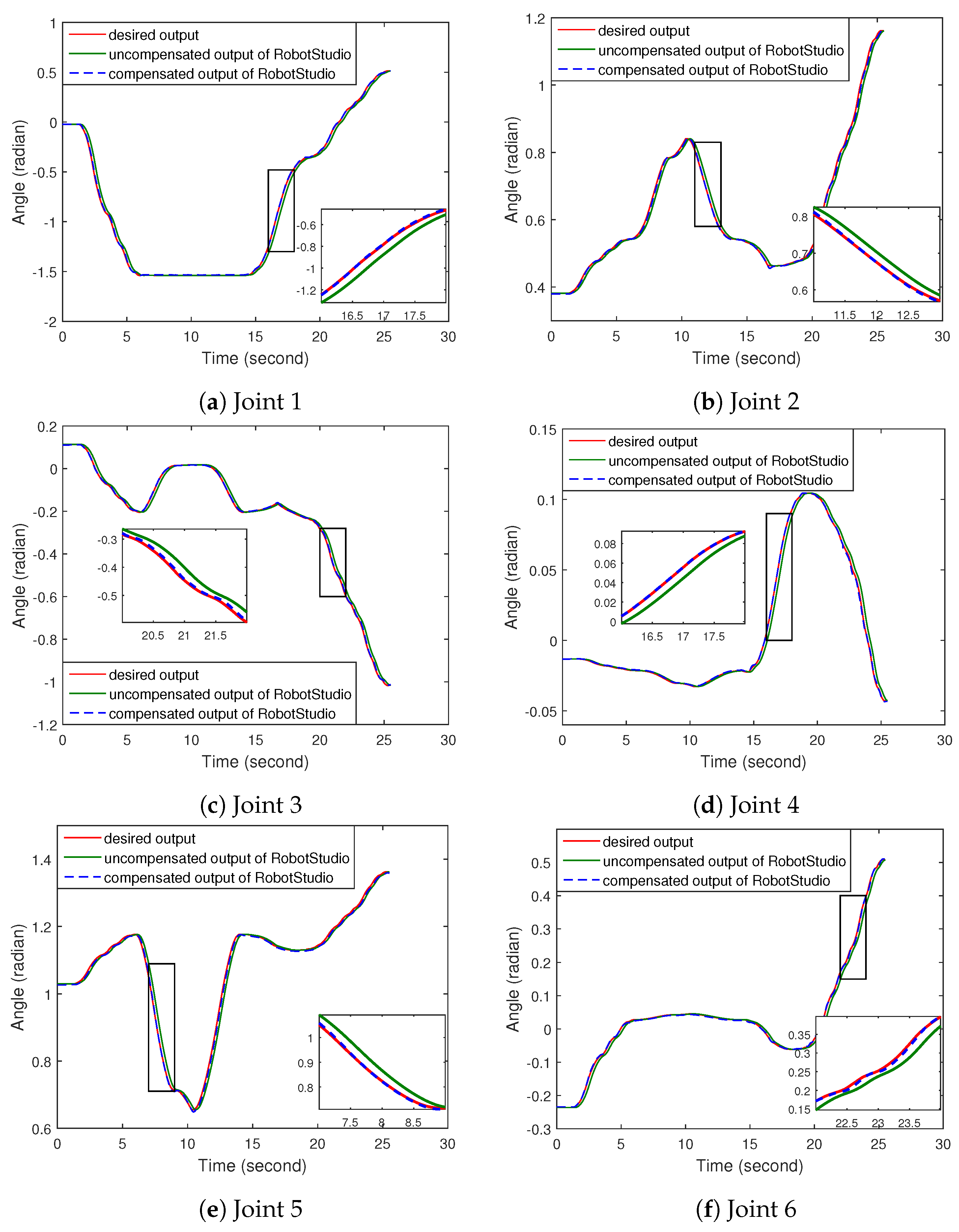
To further test the generalization capability of the trained NNs, we conducted another test of tracking 6-dimensional joint trajectories planned by MoveIt! for a large-structure assembly task [
49] in RobotStudio. The comparison of tracking performance without and with NN compensation is shown in
Figure 9.
Table 4 reports the corresponding tracking errors.
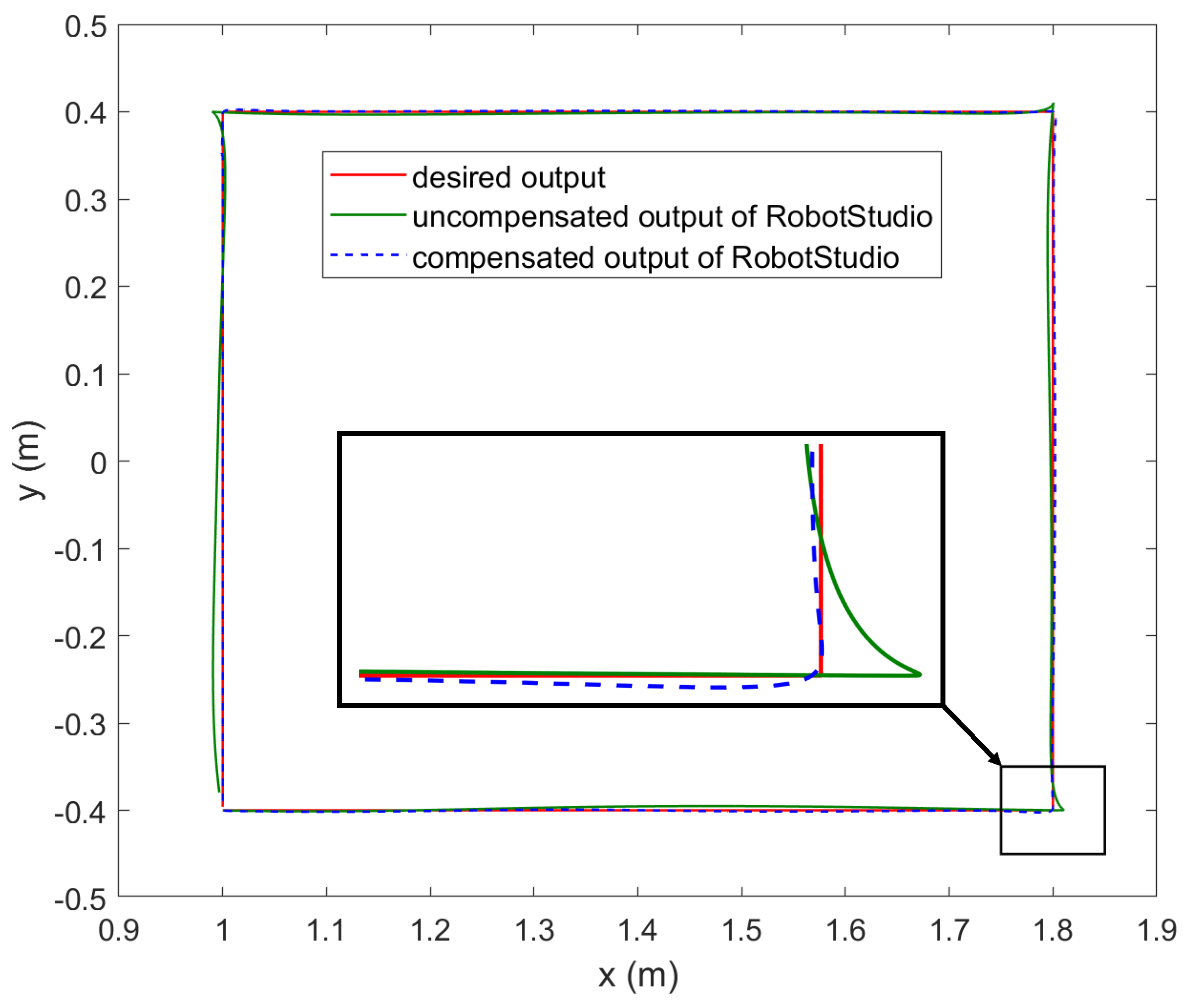
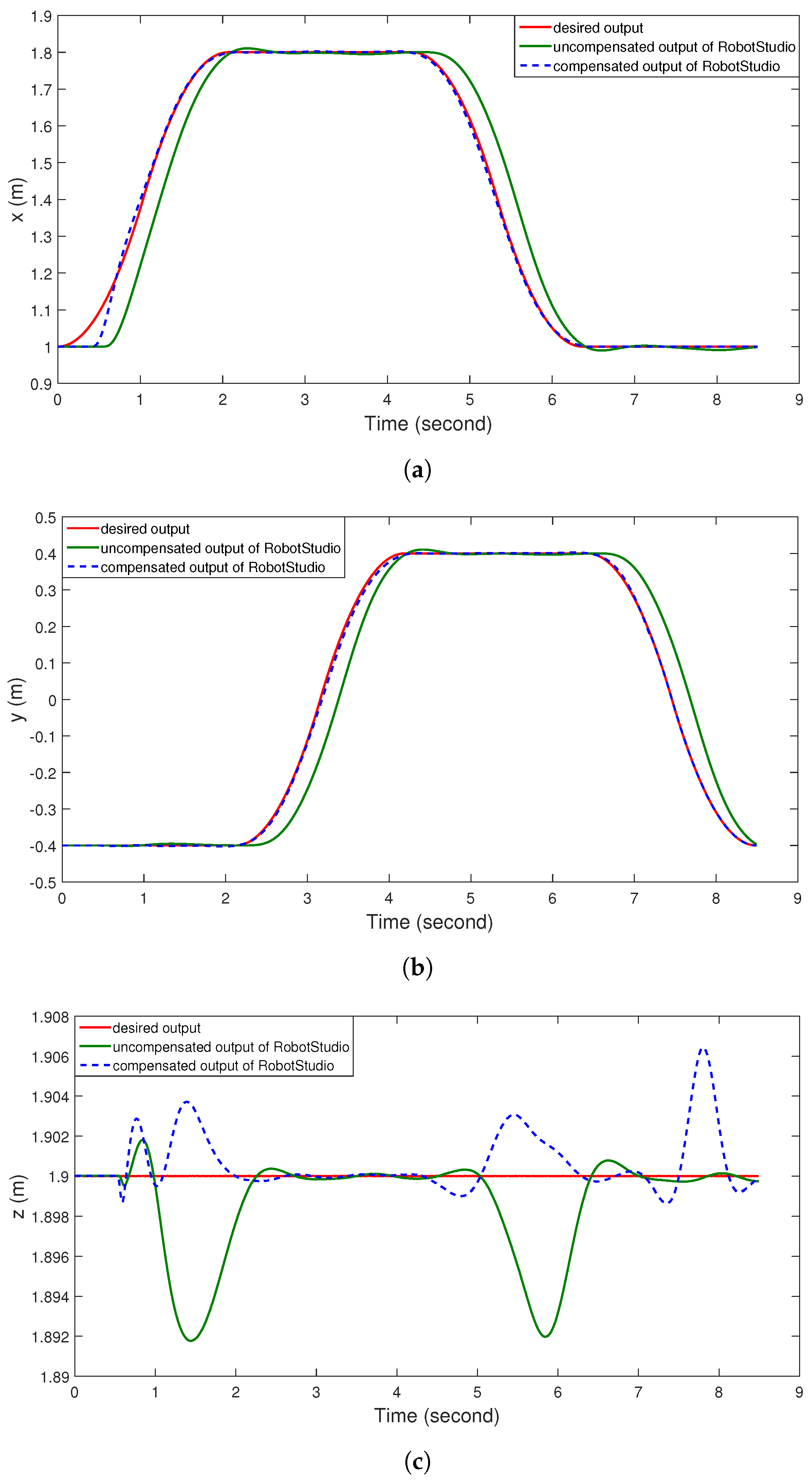
5.1.3. Cartesian Motion Tracking
We also evaluated the performance of the trained NNs on a Cartesian square trajectory (in the
x-
y plane, with a
z constant of 1.9 m) with bounded velocity and acceleration (maximum velocity of 1 m/s and a maximum acceleration of 0.75 m/s
2). During the motion, the orientation of the robot end-effector remained fixed.
Figure 10 shows that the trained NNs effectively corrected the tracking errors and
Figure 11 highlights the tracking performance in three Cartesian directions. The corresponding
norms of tracking errors in three Cartesian directions are summarized in
Table 5.
5.1.4. Comparison with MoveL Command
We also compared the NN-based compensation with built-in ABB motion command MoveL, which is used to move the tool center point linearly to a given destination. Considering the 0.6∼0.7 s initial dead time of EGM, we compared the tracking of a straight line with a total movement time of 5 s, using MoveL, EGM without NN compensation, and EGM with NN compensation, as well as running an extra 3 ILC iterations using the input generated by the NN as the initial guess
. The corresponding RMSE tracking errors are summarized in
Table 6.
The built-in motion command MoveL achieves accurate tracking, but it is for a fixed path and cannot be modified on the fly. So it is not applicable to real-time collision avoidance or sensor-based motion control. EGM, on the other hand, allows for sensor-guided motion with a high sampling rate, but the tracking performance is compromised by the delay and internal dynamics.
Table 6 indicates that the NN compensation produces a similar level of tracking performance compared with MoveL, and at the same time it retains the advantages of the sensor-guided motion of EGM.
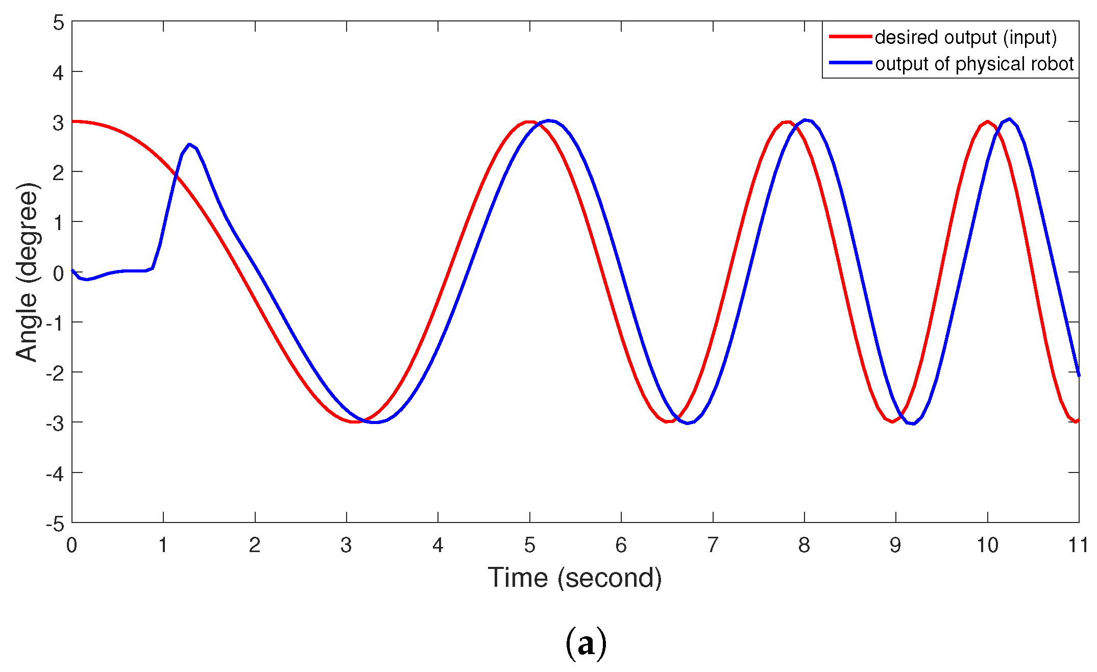
5.2. Physical Experiment Results on IRB6640-180
We evaluated the tracking performance of the same chirp signal (in
Figure 6) for joint 1 of the physical robot, as demonstrated in
Figure 12. The command input was filtered by the NNs through transfer learning.
Figure 12a shows the uncompensated output with the robot output lagging behind the desired output.
Figure 12b shows that, by compensating for the lag effect, the command input generated by the NNs drives the output to the desired output closely after a brief initial transient. We found that for trajectories with low velocity profiles (like this chirp signal and the sinusoid in
Figure 5a), there exists a negligible difference between the filtered inputs of NNs trained by simulation data and NNs obtained by transfer learning.
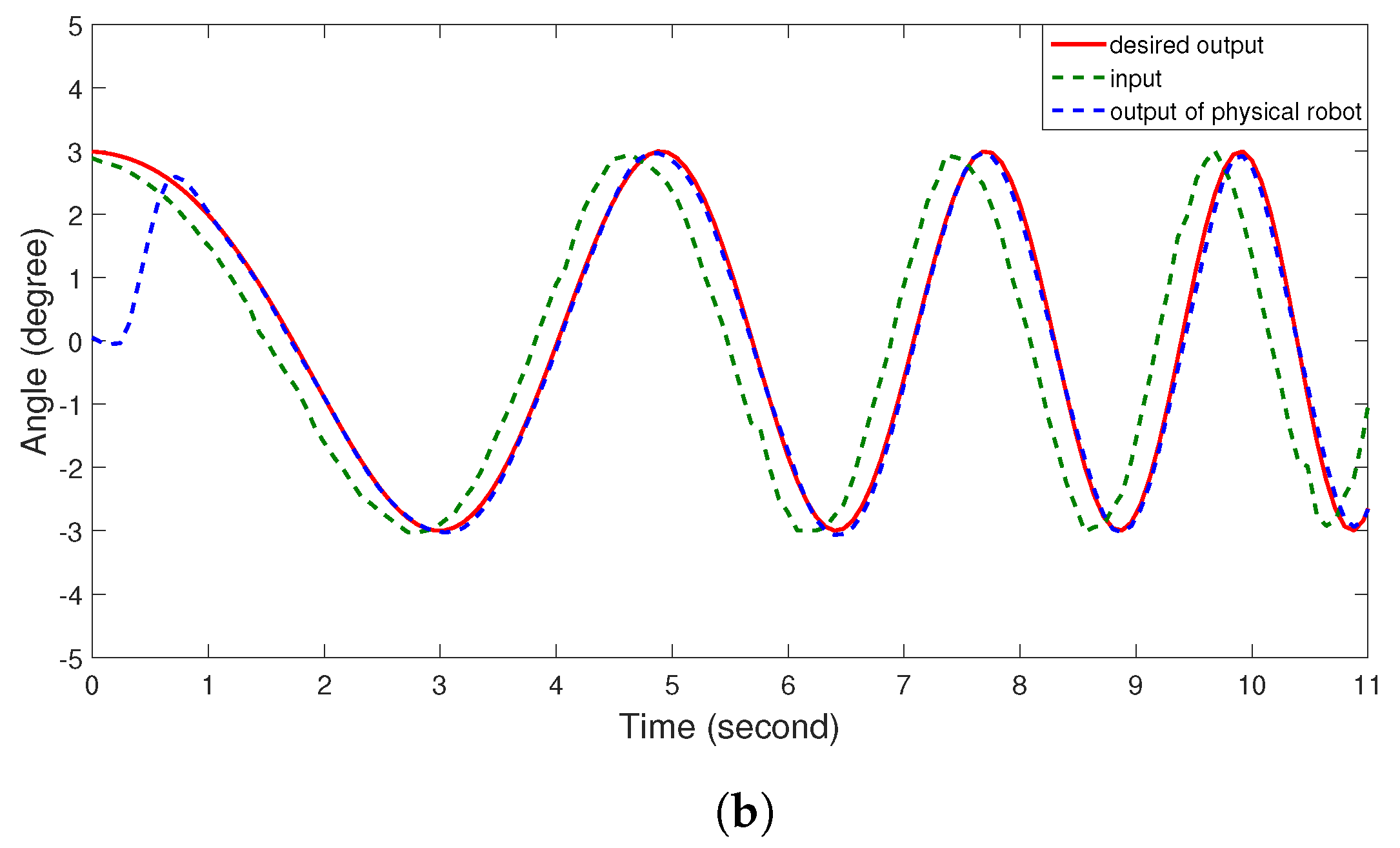
However, for trajectories with large velocity and acceleration profiles, transfer learning plays a key role in generating an optimal input to reduce trajectory tracking errors for the physical robot.
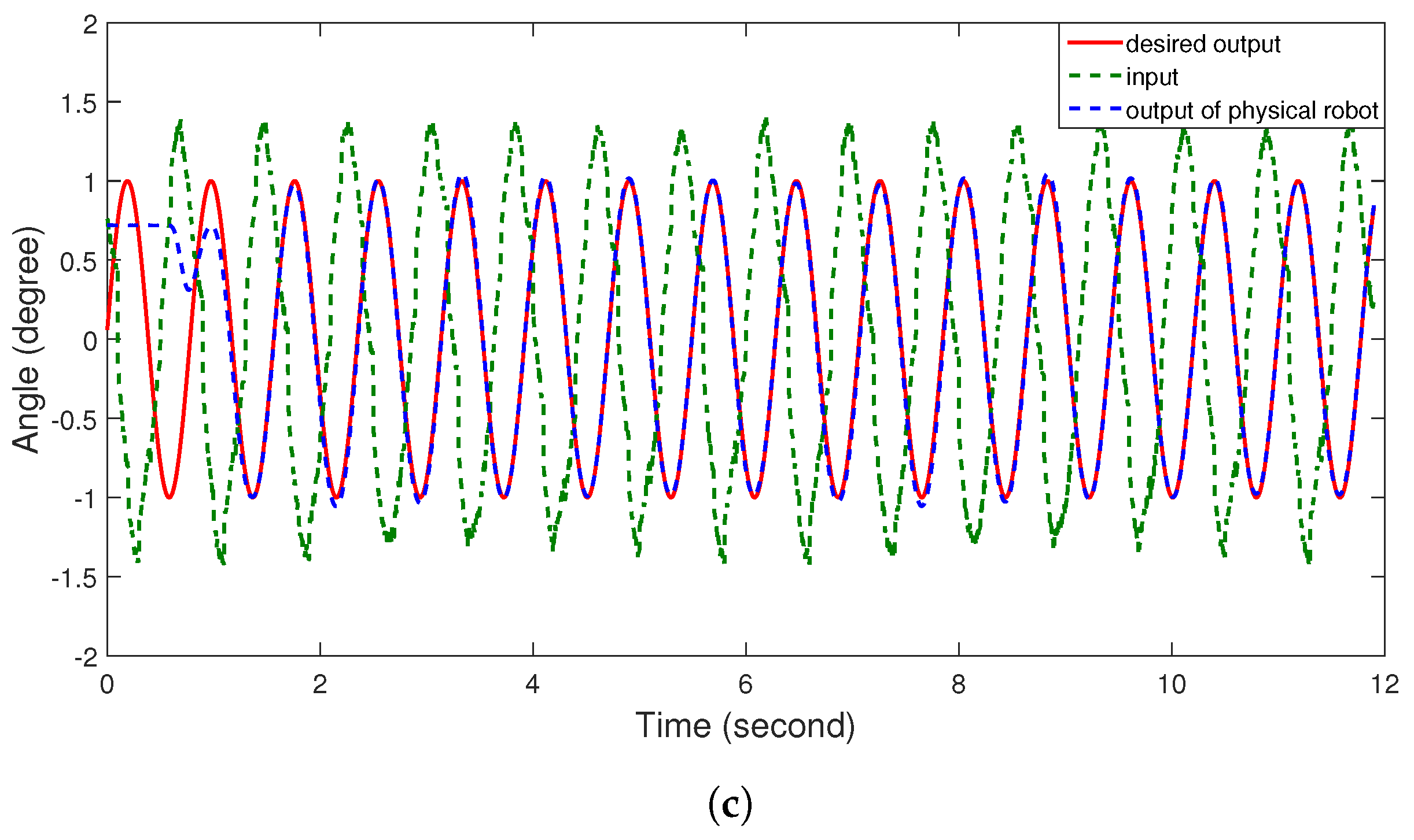
Figure 13 illustrates the tracking of a sinusoidal signal with an angular frequency of 8 rad/s (with different amplitude and phase from the training data). The comparison between
Figure 13b,c demonstrates that transfer learning is necessary to correctly compensate for the phase lagging and magnitude degradation for the physical robot given an aggressive motion profile.
Table 7 summarizes the corresponding
norms of tracking errors.
5.3. RobotStudio Simulation Results for Other Robots
One natural question that arises is whether the trained NNs also work on different robot models. We applied the trained NNs by simulation data to two robot models IRB120 and IRB6640-130 in RobotStudio, and tested their tracking on a chirp trajectory (the same one as we used in
Section 5.1.1) and a sinusoidal signal with an angular frequency of 8 rad/s and a magnitude of 5 degrees, as shown in
Figure 14.
The figure demonstrates that the trained NNs effectively compensate for the lag effect and amplitude discrepancies for these two robot models. For tracking of the chirp signal, NNs compensate for the delay well for these robots and a possible explanation for this could be that EGM has the same time delay for all robot models. For tracking of the sinusoid signal with obvious nonlinear effects, NNs compensate for both the delay and the magnitude degradation well, since their inner-loop dynamics have similar behavior to the IRB6640-180 robot.
6. Conclusions and Future Work
In this paper, the possibility of combining multi-layer NNs and ILC to achieve high-performance tracking of a 6-dof industrial robot was explored. Large amounts of data for NN training were collected by ILC in a high-fidelity physical simulator. The trained NNs generalized well to unseen trajectories and tracking performance was improved significantly. Transfer learning was adopted to narrow down the reality gap, and the generality of the NNs was further explored on two different robot models.
Future work will include the development of predictive motion and force controllers based on the trained NNs. Moreover, the tracking accuracy could be further improved by introducing feedback corrections. Finally, it will be worthwhile to compare the NNs with other neural-learning controllers, and verify the possibility of the trained NNs serving as a general dynamics compensator.
Author Contributions
Conceptualization, S.C. and J.T.W.; methodology, S.C. and J.T.W.; software, S.C.; validation, S.C.; formal analysis, S.C. and J.T.W.; investigation, S.C. and J.T.W.; resources, J.T.W.; data curation, S.C.; writing—original draft preparation, S.C.; writing—review and editing, S.C. and J.T.W.; supervision, J.T.W.; project administration, J.T.W.; funding acquisition, J.T.W. All authors have read and agreed to the published version of the manuscript.
Funding
This research was funded in part by the Office of the Secretary of Defense under Agreement Number W911NF-17-3-0004 and in part by the New York State Matching Grant program and by the Manufacturing Innovation Center (MIC) at Rensselaer Polytechnic Institute under a block grant from the New York State Empire State Development Division of Science, Technology and Innovation (NYSTAR).
Institutional Review Board Statement
Not applicable.
Informed Consent Statement
Not applicable.
Data Availability Statement
Acknowledgments
The authors would like to thank Glenn Saunders for help setting up the ABB robot testbed.
Conflicts of Interest
The authors declare no conflict of interest.
References
- Man, Z.; Palaniswami, M. Robust tracking control for rigid robotic manipulators. IEEE Trans. Autom. Control 1994, 39, 154–159. [Google Scholar] [CrossRef]
- Slotine, J.J.E.; Li, W. On the Adaptive Control of Robot Manipulators. Int. J. Robot. Res. 1987, 6, 49–59. [Google Scholar] [CrossRef]
- Spong, M.; Khorasani, K.; Kokotovic, P. An integral manifold approach to the feedback control of flexible joint robots. IEEE J. Robot. Autom. 1987, 3, 291–300. [Google Scholar] [CrossRef]
- Abiyev, R.H.; Kaynak, O. Fuzzy Wavelet Neural Networks for Identification and Control of Dynamic Plants—A Novel Structure and a Comparative Study. IEEE Trans. Ind. Electron. 2008, 55, 3133–3140. [Google Scholar] [CrossRef]
- Arimoto, S. Learning control theory for robotic motion. Int. J. Adapt. Control Signal Process. 1990, 4, 543–564. [Google Scholar] [CrossRef]
- Norrlöf, M. An adaptive iterative learning control algorithm with experiments on an industrial robot. IEEE Trans. Robot. Autom. 2002, 18, 245–251. [Google Scholar] [CrossRef]
- Visioli, A.; Legnani, G. On the trajectory tracking control of industrial SCARA robot manipulators. IEEE Trans. Ind. Electron. 2002, 49, 224–232. [Google Scholar] [CrossRef]
- Pan, S.J.; Yang, Q. A Survey on Transfer Learning. IEEE Trans. Knowl. Data Eng. 2010, 22, 1345–1359. [Google Scholar] [CrossRef]
- Williams, C.; Klanke, S.; Vijayakumar, S.; Chai, K.M. Multi-task Gaussian Process Learning of Robot Inverse Dynamics. In Advances in Neural Information Processing Systems 21; Koller, D., Schuurmans, D., Bengio, Y., Bottou, L., Eds.; Curran Associates, Inc.: Red Hook, NY, USA, 2009; pp. 265–272. [Google Scholar]
- Narendra, K.S.; Parthasarathy, K. Identification and control of dynamical systems using neural networks. IEEE Trans. Neural Netw. 1990, 1, 4–27. [Google Scholar] [CrossRef]
- Levin, A.U.; Narendra, K.S. Control of nonlinear dynamical systems using neural networks: Controllability and stabilization. IEEE Trans. Neural Netw. 1993, 4, 192–206. [Google Scholar] [CrossRef]
- Jiang, Y.; Yang, C.; Na, J.; Li, G.; Li, Y.; Zhong, J. A Brief Review of Neural Networks Based Learning and Control and Their Applications for Robots. Complexity 2017, 2017, 1895897. [Google Scholar] [CrossRef]
- Jin, L.; Li, S.; Yu, J.; He, J. Robot manipulator control using neural networks: A survey. Neurocomputing 2018, 285, 23–34. [Google Scholar] [CrossRef]
- Ouyang, Y.; Dong, L.; Wei, Y.; Sun, C. Neural network based tracking control for an elastic joint robot with input constraint via actor-critic design. Neurocomputing 2020, 409, 286–295. [Google Scholar] [CrossRef]
- Lou, W.; Guo, X. Adaptive Trajectory Tracking Control using Reinforcement Learning for Quadrotor. Int. J. Adv. Robot. Syst. 2016, 13, 38. [Google Scholar] [CrossRef]
- Jiang, Y.; Wang, Y.; Miao, Z.; Na, J.; Zhao, Z.; Yang, C. Composite-Learning-Based Adaptive Neural Control for Dual-Arm Robots With Relative Motion. IEEE Trans. Neural Netw. Learn. Syst. 2020, 1–12. [Google Scholar] [CrossRef]
- Kong, L.; He, W.; Yang, C.; Sun, C. Robust Neurooptimal Control for a Robot via Adaptive Dynamic Programming. IEEE Trans. Neural Netw. Learn. Syst. 2020, 1–11. [Google Scholar] [CrossRef] [PubMed]
- Fei, J.; Lu, C. Adaptive Sliding Mode Control of Dynamic Systems Using Double Loop Recurrent Neural Network Structure. IEEE Trans. Neural Netw. Learn. Syst. 2018, 29, 1275–1286. [Google Scholar] [CrossRef]
- Liu, Y.; Lu, S.; Tong, S. Neural Network Controller Design for an Uncertain Robot With Time-Varying Output Constraint. IEEE Trans. Syst. Man Cybern. Syst. 2017, 47, 2060–2068. [Google Scholar] [CrossRef]
- Wang, M.; Ye, H.; Chen, Z. Neural Learning Control of Flexible Joint Manipulator with Predefined Tracking Performance and Application to Baxter Robot. Complexity 2017, 2017, 7683785:1–7683785:14. [Google Scholar] [CrossRef]
- He, W.; Yan, Z.; Sun, Y.; Ou, Y.; Sun, C. Neural-Learning-Based Control for a Constrained Robotic Manipulator With Flexible Joints. IEEE Trans. Neural Netw. Learn. Syst. 2018, 29, 5993–6003. [Google Scholar] [CrossRef]
- Chen, S.; Wen, J.T. Adaptive Neural Trajectory Tracking Control for Flexible-Joint Robots with Online Learning. In Proceedings of the 2020 IEEE International Conference on Robotics and Automation (ICRA), Paris, France, 31 May–31 August 2020. [Google Scholar]
- Peng, L.; Woo, P.-Y. Neural-fuzzy control system for robotic manipulators. IEEE Control Syst. Mag. 2002, 22, 53–63. [Google Scholar] [CrossRef]
- Chen, C. Dynamic Structure Neural-Fuzzy Networks for Robust Adaptive Control of Robot Manipulators. IEEE Trans. Ind. Electron. 2008, 55, 3402–3414. [Google Scholar] [CrossRef]
- Wai, R.; Muthusamy, R. Fuzzy-Neural-Network Inherited Sliding-Mode Control for Robot Manipulator Including Actuator Dynamics. IEEE Trans. Neural Netw. Learn. Syst. 2013, 24, 274–287. [Google Scholar] [CrossRef] [PubMed]
- Lu, C. Wavelet Fuzzy Neural Networks for Identification and Predictive Control of Dynamic Systems. IEEE Trans. Ind. Electron. 2011, 58, 3046–3058. [Google Scholar] [CrossRef]
- He, W.; Dong, Y.; Sun, C. Adaptive Neural Impedance Control of a Robotic Manipulator With Input Saturation. IEEE Trans. Syst. Man Cybern. Syst. 2016, 46, 334–344. [Google Scholar] [CrossRef]
- Yang, C.; Wang, X.; Cheng, L.; Ma, H. Neural-Learning-Based Telerobot Control With Guaranteed Performance. IEEE Trans. Cybern. 2017, 47, 3148–3159. [Google Scholar] [CrossRef] [PubMed]
- Ji, Y.; Liu, D.; Guo, Y. Adaptive neural network based position tracking control for Dual-master/Single-slave teleoperation system under communication constant time delays. ISA Trans. 2019, 93, 80–92. [Google Scholar] [CrossRef] [PubMed]
- Sun, T.; Pei, H.; Pan, Y.; Zhou, H.; Zhang, C. Neural network-based sliding mode adaptive control for robot manipulators. Neurocomputing 2011, 74, 2377–2384. [Google Scholar] [CrossRef]
- Lewis, F.L.; Yesildirek, A.; Liu, K. Multilayer neural-net robot controller with guaranteed tracking performance. IEEE Trans. Neural Netw. 1996, 7, 388–399. [Google Scholar] [CrossRef] [PubMed]
- Ranatunga, I.; Cremer, S.; Lewis, F.L.; Popa, D.O. Neuroadaptive control for safe robots in human environments: A case study. In Proceedings of the 2015 IEEE International Conference on Automation Science and Engineering (CASE), Gothenburg, Sweden, 4–28 August 2015; pp. 322–327. [Google Scholar] [CrossRef]
- Liu, Z.; Chen, C.; Zhang, Y.; Chen, C.L.P. Adaptive Neural Control for Dual-Arm Coordination of Humanoid Robot With Unknown Nonlinearities in Output Mechanism. IEEE Trans. Cybern. 2015, 45, 507–518. [Google Scholar] [CrossRef]
- Wang, L.; Liu, Z.; Chen, C.L.P.; Zhang, Y.; Lee, S.; Chen, X. Energy-Efficient SVM Learning Control System for Biped Walking Robots. IEEE Trans. Neural Netw. Learn. Syst. 2013, 24, 831–837. [Google Scholar] [CrossRef] [PubMed]
- Shi, G.; Shi, X.; O’Connell, M.; Yu, R.; Azizzadenesheli, K.; Anandkumar, A.; Yue, Y.; Chung, S.J. Neural Lander: Stable Drone Landing Control using Learned Dynamics. arXiv 2018, arXiv:1811.08027. [Google Scholar]
- Noormohammadi-Asl, A.; Saffari, M.; Teshnehlab, M. Neural Control of Mobile Robot Motion Based on Feedback Error Learning and Mimetic Structure. In Proceedings of the Electrical Engineering (ICEE), Iranian Conference on, Mashhad, Iran, 8–10 May 2018; pp. 778–783. [Google Scholar] [CrossRef]
- Umlauft, J.; Hirche, S. Feedback Linearization based on Gaussian Processes with event-triggered Online Learning. IEEE Trans. Autom. Control 2019, 65, 4154–4169. [Google Scholar] [CrossRef]
- Polydoros, A.S.; Nalpantidis, L.; Krüger, V. Real-time deep learning of robotic manipulator inverse dynamics. In Proceedings of the 2015 IEEE/RSJ International Conference on Intelligent Robots and Systems (IROS), Hamburg, Germany, 8 September–2 October 2015; pp. 3442–3448. [Google Scholar] [CrossRef]
- Chaoui, H.; Sicard, P.; Gueaieb, W. ANN-Based Adaptive Control of Robotic Manipulators With Friction and Joint Elasticity. IEEE Trans. Ind. Electron. 2009, 56, 3174–3187. [Google Scholar] [CrossRef]
- Patino, H.D.; Carelli, R.; Kuchen, B.R. Neural networks for advanced control of robot manipulators. IEEE Trans. Neural Netw. 2002, 13, 343–354. [Google Scholar] [CrossRef] [PubMed]
- Selmic, R.R.; Lewis, F.L. Deadzone compensation in motion control systems using neural networks. IEEE Trans. Autom. Control 2000, 45, 602–613. [Google Scholar] [CrossRef]
- Rueckert, E.; Nakatenus, M.; Tosatto, S.; Peters, J. Learning inverse dynamics models in O(n) time with LSTM networks. In Proceedings of the 2017 IEEE-RAS 17th International Conference on Humanoid Robotics (Humanoids), Birmingham, UK, 15–17 November 2017; pp. 811–816. [Google Scholar] [CrossRef]
- ABB Robotics. Product Manual-IRB6640; ABB Robotics: Västerås, Sweden, 2010. [Google Scholar]
- ABB Robotics. Application Manual: Controller Software IRC5: RobotWare 6.04; ABB Robotics: Västerås, Sweden, 2016. [Google Scholar]
- Connolly, C. Technology and applications of ABB RobotStudio. Ind. Robot. Int. J. 2009, 36, 540–545. [Google Scholar] [CrossRef]
- Potsaid, B.; Wen, J.T.; Unrath, M.; Watt, D.; Alpay, M. High Performance Motion Tracking Control for Electronic Manufacturing. J. Dyn. Syst. Meas. Control 2007, 129, 767–776. [Google Scholar] [CrossRef][Green Version]
- Chen, S.; Wang, Z.; Chakraborty, A.; Klecka, M.; Saunders, G.; Wen, J.T. Robotic Deep Rolling With Iterative Learning Motion and Force Control. IEEE Robot. Autom. Lett. 2020, 5, 5581–5588. [Google Scholar] [CrossRef]
- Noriega, J.R.; Wang, H. A direct adaptive neural-network control for unknown nonlinear systems and its application. IEEE Trans. Neural Netw. 1998, 9, 27–34. [Google Scholar] [CrossRef]
- Chen, S.; Peng, Y.C.; Wason, J.; Cui, J.; Saunders, G.; Nath, S.; Wen, J.T. Software Framework for Robot-Assisted Large Structure Assembly. In Proceedings of the ASME 2018 13th International Manufacturing Science and Engineering Conference, College Station, TX, USA, 18 June 2018. [Google Scholar]
Figure 1.
Overview of the neural-learning trajectory tracking control approach.
Figure 1.
Overview of the neural-learning trajectory tracking control approach.
Figure 2.
Robot dynamics with closed loop joint servo control. The goal of the neural-learning control approach is to find a possibly non-causal feedforward compensator using MNNs.
Figure 2.
Robot dynamics with closed loop joint servo control. The goal of the neural-learning control approach is to find a possibly non-causal feedforward compensator using MNNs.
Figure 3.
Trajectory tracking improvement with iterative refinement after 8 iterations. The desired trajectory is a sinusoid with ω = 3 rad/s. (a) Desired output (also the input to externally guided motion (EGM)), RobotStudio output, and linear model output. (b) Desired output, RobotStudio output, and modified input based on iterative refinement.
Figure 4.
The architecture of the employed neural network that has two fully-connected hidden layers and 100 nodes in each hidden layer. The input and output layer contains 50 and 25 nodes, respectively.
Figure 4.
The architecture of the employed neural network that has two fully-connected hidden layers and 100 nodes in each hidden layer. The input and output layer contains 50 and 25 nodes, respectively.
Figure 5.
Comparison of responses between RobotStudio (red curve) and the physical robot (blue curve). Desired inputs are sinusoids with amplitude of 2° and angular frequency ω of 2 rad/s (a) and 10 rad/s (b). (a) RobotStudio captures the dynamics of the physical robot well when commanded a slow trajectory. (b) Discrepancy exists between RobotStudio dynamics and the physical robot when commanded a fast trajectory.
Figure 6.
Comparison of tracking performance without and with the NN compensation for a chirp signal in RobotStudio. TheNNfeedforward controller addresses the issues of lag effect and amplitude discrepancies induced by robot inner loop dynamics. (a) Uncompensated case: desired output (also the input into EGM), RobotStudio output, and linear model output. (b) Compensation with NN: desired output, RobotStudio output, and the input generated by the NN.
Figure 7.
Comparison of tracking performance with and without the NN compensation of a random joint trajectory for joint 1 in RobotStudio. The generalization capability of the NN feedforward controller is demonstrated through the improved tracking accuracy.
Figure 7.
Comparison of tracking performance with and without the NN compensation of a random joint trajectory for joint 1 in RobotStudio. The generalization capability of the NN feedforward controller is demonstrated through the improved tracking accuracy.
Figure 8.
Comparison of tracking performance with and without the NN compensation of a multi-joint sinusoidal trajectory in RobotStudio. The NN feedforward controller improves the trajectory tracking accuracy for all 6 joints.
Figure 8.
Comparison of tracking performance with and without the NN compensation of a multi-joint sinusoidal trajectory in RobotStudio. The NN feedforward controller improves the trajectory tracking accuracy for all 6 joints.
Figure 9.
Comparison of tracking performance with and without the NN compensation of the MoveIt! planned joint trajectories in RobotStudio. The inset figures clearly demonstrate the improvement of tracking.
Figure 9.
Comparison of tracking performance with and without the NN compensation of the MoveIt! planned joint trajectories in RobotStudio. The inset figures clearly demonstrate the improvement of tracking.
Figure 10.
Comparison of tracking performance without and with the NN compensation of a Cartesian square trajectory in the
x-
y plane with
z constant in RobotStudio. The improved tracking performance of each Cartesian axis is reported in
Table 5.
Figure 10.
Comparison of tracking performance without and with the NN compensation of a Cartesian square trajectory in the
x-
y plane with
z constant in RobotStudio. The improved tracking performance of each Cartesian axis is reported in
Table 5.
Figure 11.
Improved tracking performance of
Figure 10 in individual Cartesian axis. With the NN compensation, the tracking errors are significantly reduced for all axes, as reported in
Table 5. (
a) Tracking performance in
x. (
b) Tracking performance in
y. (
c) Tracking performance in
z.
Figure 11.
Improved tracking performance of
Figure 10 in individual Cartesian axis. With the NN compensation, the tracking errors are significantly reduced for all axes, as reported in
Table 5. (
a) Tracking performance in
x. (
b) Tracking performance in
y. (
c) Tracking performance in
z.
Figure 12.
Comparison of the tracking performance of the same chirp signal as the one in the simulation (
Figure 6) without and with the NN compensation for joint 1 of the physical robot. (
a) Uncompensated case: desired output (also the input into EGM) and the physical robot output. (
b) Compensation with NN: desired output, physical robot output, and the input generated by the NN.
Figure 13.
Comparison of tracking performance of a sinusoidal trajectory without and with transfer learning for joint 1 of the physical robot. The
norm of the tracking error of each case is shown in
Table 7. Transfer learning plays a key role for tracking a fast trajectory. (
a) No NN compensation. (
b) Compensation using the NN trained by the simulation data. (
c) Compensation using the NN tuned by transfer learning.
Figure 14.
The trained NNs using IRB6640-180 also improve the tracking accuracy of a chirp and a sinusoidal joint trajectories for IRB120 and IRB6640-130 robots in RobotStudio, possibly because these robots have similar inner loop dynamics.
Figure 14.
The trained NNs using IRB6640-180 also improve the tracking accuracy of a chirp and a sinusoidal joint trajectories for IRB120 and IRB6640-130 robots in RobotStudio, possibly because these robots have similar inner loop dynamics.
Table 1.
Comparison of the norm of tracking errors for a single-joint trajectory, by using iterative refinement implemented with RobotStudio and with the fitted linear model . The initial tracking error was 31.6230. The linear model offers a reliable approximation of the EGM linear region.
Table 1.
Comparison of the norm of tracking errors for a single-joint trajectory, by using iterative refinement implemented with RobotStudio and with the fitted linear model . The initial tracking error was 31.6230. The linear model offers a reliable approximation of the EGM linear region.
| Iteration # | Tracking Error | Tracking Error |
|---|
| | Using RobotStudio (°) | Using Linear Model (°) |
|---|
| 1 | 26.0699 | 25.0585 |
| 2 | 21.0735 | 20.0049 |
| 3 | 17.1372 | 15.9724 |
| 4 | 13.6738 | 12.7540 |
| 5 | 11.2821 | 10.1849 |
Table 2.
Mean squared testing error of different NN architectures. The architecture with two hidden layers and 100 nodes in each hidden layer produces the best accuracy.
Table 2.
Mean squared testing error of different NN architectures. The architecture with two hidden layers and 100 nodes in each hidden layer produces the best accuracy.
Number of
Hidden Layers | Number of Nodes
in Each Layer | Final Testing Error (°)
(Mean of Three Tests) |
|---|
| 2 | 50/100 100/100 | 2.623 2.145 |
| 2 | 100/150 100/200 | 2.474 2.545 |
| 3 | 100/100/100 100/150/100 | 2.390 2.486 |
| 4 | 100/100/100/50 | 2.450 |
Table 3.
and norm of tracking errors of the 6-dimensional sinusoidal joint trajectory without and with NN compensation in RobotStudio. The tracking performance is improved for all 6 joints with NN compensation.
Table 3.
and norm of tracking errors of the 6-dimensional sinusoidal joint trajectory without and with NN compensation in RobotStudio. The tracking performance is improved for all 6 joints with NN compensation.
| Joint | Original Tracking Error (rad) | Final Tracking Error (rad) |
|---|
| | | | | |
|---|
| 1 | 1.4944 | 0.0391 | 0.2056 | 0.0035 |
| 2 | 2.9935 | 0.0780 | 0.4993 | 0.0065 |
| 3 | 6.1128 | 0.1563 | 0.8384 | 0.0101 |
| 4 | 1.5143 | 0.0390 | 0.1421 | 0.0038 |
| 5 | 3.0542 | 0.0781 | 0.4555 | 0.0065 |
| 6 | 5.9629 | 0.1561 | 0.8245 | 0.0102 |
Table 4.
and norm of tracking errors of MoveIt! planned joint trajectories without and with NN compensation in RobotStudio. The NN feedforward controller improves the trajectory tracking accuracy for all joints.
Table 4.
and norm of tracking errors of MoveIt! planned joint trajectories without and with NN compensation in RobotStudio. The NN feedforward controller improves the trajectory tracking accuracy for all joints.
| Joint | Original Tracking Error (rad) | Final Tracking Error (rad) |
|---|
| | | | | |
|---|
| 1 | 3.5937 | 0.1497 | 0.5959 | 0.0278 |
| 2 | 1.3251 | 0.0443 | 0.3992 | 0.0180 |
| 3 | 1.4463 | 0.0493 | 0.2846 | 0.0112 |
| 4 | 0.3303 | 0.0127 | 0.0542 | 0.0033 |
| 5 | 1.4650 | 0.0511 | 0.4773 | 0.0154 |
| 6 | 0.9629 | 0.0392 | 0.1894 | 0.0078 |
Table 5.
norm of tracking errors in three Cartesian axes. The NN feedforward controller improves the trajectory tracking accuracy in all Cartesian directions.
Table 5.
norm of tracking errors in three Cartesian axes. The NN feedforward controller improves the trajectory tracking accuracy in all Cartesian directions.
| Cartesian Axes | Original Tracking Error (m) | Final Tracking Error (m) |
|---|
| x | 3.2794 | 0.7938 |
| y | 3.1475 | 0.2490 |
| z | 0.1338 | 0.0737 |
Table 6.
RMSE tracking errors of a straight line using 4 different approaches in RobotStudio. A similar tracking accuracy to MoveL is achieved by running 3 extra ILC iterations using the commanded trajectory produced by the NNs as an initial guess for the iterative refinement in (
1).
Table 6.
RMSE tracking errors of a straight line using 4 different approaches in RobotStudio. A similar tracking accuracy to MoveL is achieved by running 3 extra ILC iterations using the commanded trajectory produced by the NNs as an initial guess for the iterative refinement in (
1).
| RMSE (m) | MoveL | EGM without NN | EGM with NN | Extra ILCs |
|---|
| x | 0.0027 | 0.0200 | 0.0110 | 0.0083 |
| y | 0.0027 | 0.0200 | 0.0104 | 0.0081 |
| z | 0.0027 | 0.0200 | 0.0105 | 0.0081 |
Table 7.
norm of tracking errors in radian for each subplot in
Figure 13. The table demonstrates the improved tracking performance using transfer learning for tracking a fast trajectory.
Table 7.
norm of tracking errors in radian for each subplot in
Figure 13. The table demonstrates the improved tracking performance using transfer learning for tracking a fast trajectory.
| Uncompensated Case | Without Transfer Learning | With Transfer Learning |
|---|
| 1.0242 | 0.2445 | 0.2388 |
| Publisher’s Note: MDPI stays neutral with regard to jurisdictional claims in published maps and institutional affiliations. |
© 2021 by the authors. Licensee MDPI, Basel, Switzerland. This article is an open access article distributed under the terms and conditions of the Creative Commons Attribution (CC BY) license (http://creativecommons.org/licenses/by/4.0/).


