A Program Library for Computing Pure Spin-Angular Coefficients for One- and Two-Particle Operators in Non-Relativistic Atomic Theory

Abstract

A program library, libang77, for computing pure spin-angular coefficients for any one- and scalar two-particle operator is presented. The method is based on the combination of the second quantization and quasi-spin techniques with angular momentum theory and the method of irreducible tensorial sets. A non-relativistic approach is used, in which relativistic corrections may be included in the Breit–Pauli approximation. This program library, libang77, is integrated into the Atomic Structure Package ATSP2K [ATSP2K, C. Froese Fischer, G. Tachiev, G. Gaigalas, and M.R. Godefroid, Comput. Phys. Commun. (2007). DOI: 10.1016/j.cpc.2007.01.006], but it can be implemented in other program packages too.

1. Introduction

Models of many-electron atoms and ions require both relativistic and correlation effects to be taken into account to obtain very precise characteristics of atoms and ions. This can be done, for example, by using the multiconfiguration Hartree–Fock (MCHF) method, the configuration interaction (CI) method, various versions of perturbation theory, or the semi-empirical method [1,2,3]. All of them require the calculation of matrix elements of physical operators or effective operators from perturbation theory. The symmetry properties of atomic states allow the calculation of matrix elements to be divided into the calculation of spin-angular terms and the accompanying radial integrals. The latter are more straightforward and can be handled by methods such as those used in the ATomic Structure Package (Atsp) [1,4,5,6]. Such packages have a modular structure, and the modules for calculating the spin-angular part for matrix elements of any operator can easily be replaced with a new package, which can be more efficient for large-scale computation of open shell atoms.

Many existing codes for integrating the spin-angular part for matrix elements of any operator are based on the Fano scheme [7]. The integrations over spin-angular variables in this case constitute a considerable part of the problem, especially when atoms with many open shells are treated, and the operators are non-trivial. The efficient approach for finding reduced matrix elements of any one- and two-particle atomic operator between complex configurations were developed between 1994 and 2004 (over decades) (see papers: Gaigalas and Rudzikas [8] (hereafter referred to as P1), Gaigalas et al.  [9] (hereafter referred to as P2), Gaigalas et al. [10] (hereafter referred to as P3), Gaigalas et al. [11] (hereafter referred to as P4), Gaigalas [12] (hereafter referred to as P5), Gaigalas [13] (hereafter referred to as P6), Gaigalas et al. [14] (hereafter referred to as P7), and Gaigalas [15] (hereafter referred to as P8).

P1 presents all the necessary prerequisites for the creation of a new effective method for integrating the spin-angular part of reduced matrix elements of one- and two-particle operators.

This new efficient method for spin-angular integration is developed and described in detail in P2. It is based on the combination of the angular momentum theory as described in Jucys and Bandzaitis [16], on the concept of irreducible tensorial sets (Judd [17], and Rudzikas and Kaniauskas [18]), on a generalized graphical approach (Gaigalas et al. [19]), on the second quantization in coupling tensorial form (Rudzikas and Kaniauskas [18]), on the quasi-spin approach (Rudzikas [2]), and on the use of reduced coefficients of fractional parentage (Rudzikas [2] and Judd [17]). All reduced matrix elements (diagonal and off-diagonal with respect to configurations) differ only by the values of the projections of the quasi-spin momenta of separate shells and are expressed in terms of completely reduced matrix elements (in all three spaces) of the second quantization operators. As a result, it allows us to use standard quantities uniformly for both diagonal and off-diagonal completely reduced matrix elements. All this, in its entity, introduces a number of new features, in comparison with traditional spin-angular integration approaches.

The tensorial form of the spin–other orbit interaction operator in the formalism of second quantization is presented in P3. Such an expression is needed to calculate both diagonal and off-diagonal completely reduced matrix elements according to the approach introduced in P2. Some special cases are shown for which the tensorial structure of the spin–other orbit interaction operator reduces to an unusually simple form.

In P4, tables are presented for the reduced (in quasi-spin space) coefficients of fractional parentage (also termed as subcoefficients) for the $p^w$, $d^w$, and $f^w$ shells of equivalent electrons (electronic shells). Starting with these tables, one can utilize the quasi-spin formalism efficiently for the calculation of the energy spectra and other properties of any atom or ion of the periodic table, including any open $f^w$ shell atom. Properties of reduced coefficients of fractional parentage as well as summation rules are also discussed.

A review of methods for finding general expressions of reduced matrix elements (off-diagonal with respect to configurations included) of any one- and two-particle operator for an arbitrary number of shells in an atomic configuration is given in P5. These methods are compared in various aspects, and the advantages or shortcomings of each particular method are discussed. The efficient method published in P2 is compared with traditional methods for calculations of the spin-angular part of reduced matrix elements as well.

The general tensorial form of the orbit–orbit interaction operator in the formalism of second quantization is presented in P6. Such an expression is needed to calculate both diagonal and off-diagonal reduced matrix elements with respect to configuration in a uniform way according to the approach introduced in P2. Some special cases are shown for which the orbit–orbit interaction operator reduces to a simple form.

The general tensorial form of the hyperfine interaction operator in the formalism of second quantization is presented in P7. The methodology published in P2 and P7 allows us to account for correlation effects efficiently and, therefore, to study the hyperfine interactions in complex many-electron atoms, those with open f-shells included, in a practical manner. All this will lead us to design an efficient program for large-scale calculations of hyperfine structures.

An extension of P2 and P3 is presented in P8 for finding algebraic expressions for the spin-angular part of reduced matrix elements of any one- and two-particle operator for an arbitrary number of shells in an atomic configuration. This extension is related, at first, to a change in the definition of tensorial structure, where a non-scalar with respect to l and s space of any two-particle operator acts on four different shells. This leads to more efficient expressions for the recoupling matrices and amplitudes, which are presented in P8. In addition, P8 presents new expressions for some of the recoupling matrices, in which 6j- and 9j-coefficients are summed up algebraically. All this leads to a significantly simpler and faster calculation of the spin-angular parts for any non-scalar two-particle operator particular for such operators as spin–other orbit and spin–spin.

P1–P8 form the core of papers that describe the entire methodology for calculating reduced matrix elements (with particular attention paid to spin-angular integration in atomic theory), which is fully implemented in the software library libang77 presented in this paper. This library can treat configurations with open $f^w$ shells, is free of the shortcomings of previous approaches, extends the program’s capabilities, and has led to faster execution of spin-angular integrations. In writing this software library libang77, the aim was to preserve the external appearance of the Atsp [1,4,5,6] program as closely as possible and to maintain the input and output data formats similar to those of the previous versions, for user convenience. It is installed in the new version of the Atsp software program named the Atsp2K computer package [20], and the library itself, like the entire Atsp2K, is written in the Fortran 77 programming language. Since the libang77 library is integrated into the Atsp2K software package [20], the library and the programs that use it, along with their descriptions, are available in the Atsp repositories on GitHub of the Computational Atomic Structure group. The libang77 library has a relativistic counterpart, librang90 [21], which is based on the same spin-angular integration methodology developed in P1, P2, P5, P7, P8, and Gaigalas et al. [22] and is installed in the Grasp-2018 software package [23].

The development of the methodology and software library presented in the current paper took place from 1982 to 2010. The initial aspects of the methodology were tackled in the author’s graduation paper (under the supervision of Prof. Antanas Rimvidas Bandzaitis and Habil. Dr. Julius Kaniauskas), which was successfully defended at Vilnius University in 1982. Thereafter, when developing Rayleigh–Schrödinger Many-Body Perturbation Theory (RSMBPT) in an irreducible tensorial form during a PhD research study (under the supervision of Prof. Zenonas Rokus Rudzikas), the problem of integration of spin-angular variables into atomic theory arose, and it was successfully solved for RSMBPT in the case of atoms and ions with two open shells, which was presented in the author’s PhD thesis [24]. The methodology was extended in the general case to any atom and ion with any number of open shells (including the f-shell) for any one- and two-particle operators in non-relativistic (including the Breit–Pauli approximation) and relativistic cases, during long-term visits, in cooperation with Prof. Charlotte Froese Fischer (1929–2024) (Vanderbilt University and NIST), Prof. Ian Philip Grant (1930–2025) (University of Oxford), Prof. Michel R. Godefroid (Universite Libre De Bruxelles), Stephan Fritzsche (Kassel University), and Prof. Chenzhong Dong (Lanzhou Northwest Normal University), as well as in cooperation with Prof. Per Jönson (Malmö University), Prof. Jacek Bieroń (Uniwersytet Jagielloński), and Prof. Zenonas Rokus Rudzikas (1940−2011) (Vilnius University). This cooperation led to the successful development of the method for spin-angular integration in atomic physics, P1–P8, and its implementation in several computer software packages. A brief description of the software packages in which the methodology from P1–P8 is implemented can be found in Subsection 2.4.3 of [21].

The theoretical background from P1–P8 used in the program library libang77 is presented in Section 2. The structure of the software library libang77, its documentation with a description of main subroutines, and the library itself are presented in Section 3. The library is integrated in the Atsp2K package [20] to calculate energy structure and such atomic properties as hyperfine structures, transition parameters, and isotope shift [1,2,25] (described in Section 4), but it can be implemented in other program packages too (see Section 5). Limitations of the program library libang77 and conclusions are presented in Section 6 and Section 7, respectively.

2. Theoretical Background

2.1. Various Conventions in Atomic Theory

2.1.1. The Phase System

In this paper, as well as in P1–P8 and [20,21,23], we use the definition of tensorial product of two tensor operators as defined in (B.3.140) of [26] or (5.12) of [2] with the following definition

$$\begin{array}{c}\hfill T_q^{\left(k\right)†}={\left(-1\right)}^{k-q}{T}_{-q}^{\left(k\right)}\end{array}$$

(1)

of the tensorial operator $T^{\left(k\right)†}$ adjoint to $T^{\left(k\right)}$ (see (B.3.142) of [26] or (4) of [2]). This is the so-called standard or Fano–Racah [27] phase system. The diversity of the phase systems in atomic theory is discussed in Section 13.6 of [2]. A brief overview of the phase system definitions used in different books can be found in Section 2-5 (note 7) of [28] and in Section 1.3 of [29]. Relationships between the standard and pseudo-standard phase systems for some quantities can be found in Section 11-4 (note 7), in Section 13-9 (note 11), and in Section 16-7 of [28], as well as on page 447 of [30].

It should be noted that no matter what phase system is used in the theoretical analysis, if it is used consistently throughout the entire theory, the results will always be correct. The important thing is to keep to the same phase system in the theoretical examination.

The current paper, as well as P1–P8 [20,21,23], follow the notation used by Jucys and Savukynas [30], and Rudzikas  [2] (see Section 13.6 of [2]) that in the standard phase system, the tensor rank is written in parentheses, whereas in the pseudo-standard or Condon–Shortley [31] phase system, the parentheses are omitted. Such notations make it easy to identify at a glance which phase system is used by the authors.

2.1.2. Phase Convention for Coefficients of Fractional Parentage

In modern physics, the atomic state function of an atom is built from the configuration state functions, where the latter are antisymmetrized wave functions of separate shells, and this antisymmetrization is done via coefficients of fractional parentage (CFP). The shells are coupled to one another via their angular momenta. This allows us to use Racah algebra [32,33,34,35,36] on the level of CFP or unit tensors. In the general case, to find the values of the reduced matrix elements of any physical operator, one needs to know the values of the CFP. The latter values are tabulated and can be found in various sources (see Racah [34], Nielson and Koster [37], Slater [38], and Cowan [28]). There are also algebraic expressions (see Kaniauskas et al. [39]) for the CFPs in $LS$-coupling when the seniority quantum number $\nu$ is sufficient for the one-to-one classification of the terms, i.e., for $p^w$, $d^w$ (all w values), and $f^w$ ($0<w\le 4$, $10\le w\le 14$). But, these expressions are rather complicated and, therefore, of little use.

Typically, the CFP tabulations are only provided for shells that are partially filled. For shells that are almost filled, the CFP is found using formulas that include the configuration state function (CSF) for shells that are partially fulled. However, these formulas allow for freedom of choice in terms of phase as for definition (1). Therefore, extremely important, in addition to the definition of the phase system (see Section 2.1.1) in atomic theory, is the definition of the relation between CFP of partially $l^w$ and almost filled $l^{4l+2-w}$ shells of equivalent electrons (here, $w\le 2l+1$):

$$\begin{array}{c}\hfill \left(\left.\left.l^{4l+1-w}{\alpha }^{\prime }{Q}^{\prime }{L}^{\prime }{S}^{\prime }\right|\right\}{l}^{4l+2-w}\alpha QLS\right)\\ \hfill ={\left(-1\right)}^{\gamma }\sqrt{{\displaystyle \frac{\left(w+1\right)\left(2L^{\prime }+1\right)\left(2S^{\prime }+1\right)}{\left(4l+2-w\right)\left(2L+1\right)\left(2S+1\right)}}}\left(\left.\left.l^w\alpha QLS\right|\right\}{l}^{w+1}{\alpha }^{\prime }{Q}^{\prime }{L}^{\prime }{S}^{\prime }\right),\end{array}$$

(2)

where the phase $\gamma$ may be defined in different ways. For example, Racah [34], Wybourne [40], Cowan [28], and Sobel’man [41] used $\gamma =S+S^{\prime }+L+L^{\prime }-l-{\displaystyle \frac{1}{2}}$; Judd [17] defined it as $\gamma =S+S^{\prime }+L+L^{\prime }-l-{\displaystyle \frac{1}{2}}+{\displaystyle \frac{1}{2}}({\nu }^{\prime }+\nu +1)$; and Jucys and Savukynas [30] presented it as $\gamma =S+S^{\prime }+L+L^{\prime }-l-{\displaystyle \frac{1}{2}}+{\displaystyle \frac{1}{2}}({\nu }^{\prime }+\nu +1)+w$.

The use of different phases in Formula (2) may cause some inconsistencies and contradictions in the theoretical atomic spectroscopy. Fortunately, starting with the quasi-spin methodology (see Section 2.2), one finds this phase simply equal (see Kaniauskas et al. [42])

$$\begin{array}{c}\hfill \gamma =S+S^{\prime }+L+L^{\prime }-l-{\displaystyle \frac{1}{2}}+{\displaystyle \frac{1}{2}}\left({\nu }^{\prime }+\nu -1\right)\equiv S^{\prime }-S+L^{\prime }-L+l+{\displaystyle \frac{1}{2}}\left(\nu -{\nu }^{\prime }\right).\end{array}$$

(3)

The latter definition of $\gamma$ is the only one that is compatible with the inclusion of most symmetry in atomic theory (i.e., using tensorial algebra in the l, s, and q spaces). For more details, see P4. This (3) definition is used in the current paper, as well as in P1–P8 and [20]. I would also like to emphasize that in the previous versions of the Atsp software package [1,4,5,6], the Racah $\gamma$ definition [34] was used.

2.1.3. The Definitions of Reduced Matrix Element

The Wigner–Eckart equation plays a fundamental role in atomic theory:

$$\begin{array}{c}\hfill \left(\alpha jm\left|T_q^{\left(k\right)}\right|{\alpha }^{\prime }{j}^{\prime }{m}^{\prime }\right)\\ \hfill ={\displaystyle \frac{{(-1)}^{2k}}{\sqrt{2j+1}}}\left[\begin{array}{ccc}{j}^{\prime }& k& j\\ m^{\prime }& q& m\end{array}\right]\left(\alpha j∥T^{\left(k\right)}∥{\alpha }^{\prime }{j}^{\prime }\right)={\displaystyle \frac{{(-1)}^{2k}}{\sqrt{2j+1}}}〈j^{\prime }k{m}^{\prime }q\left|j^{\prime }kjm\right.〉\left(\alpha j∥T^{\left(k\right)}∥{\alpha }^{\prime }{j}^{\prime }\right)\\ \hfill ={(-1)}^{j-m}\left(\begin{array}{ccc}j& k& j^{\prime }\\ -m& q& m^{\prime }\end{array}\right)\left(\alpha j∥T^{\left(k\right)}∥{\alpha }^{\prime }{j}^{\prime }\right),\end{array}$$

(4)

where $\left[\begin{array}{ccc}{j}^{\prime }& k& j\\ m^{\prime }& q& m\end{array}\right]$ and $〈j^{\prime }k{m}^{\prime }q\left|j^{\prime }kjm\right.〉$ is the Clebsch–Gordan coefficient in different notations [1,2,29,31] and $\left(\begin{array}{ccc}j& k& j^{\prime }\\ -m& q& m^{\prime }\end{array}\right)$ is the $3j$-symbol (Wigner coefficient) [1,2,28].

As we can see from expression (4), we use Racah’s definition [33] of reduced matrix element $\left(\alpha j∥T^{\left(k\right)}∥{\alpha }^{\prime }{j}^{\prime }\right)$ in the current paper, as well as in P1–P8 and [20,21,23]. P1–P8 [20,21,23], and the current paper follow Jucys and Bandzaitis’s [16] (see Section 37) as well as Jucys and Savykynas’s [30] notation (see Section 2), where the reduced matrix element in the Racah’s definition [33] is written in parentheses and the reduced matrix element in the Rose’s [43] definition is written in square brackets as $\left[\alpha j∥T^{\left(k\right)}∥{\alpha }^{\prime }{j}^{\prime }\right]$. Such notations make it easy to identify at a glance which notation of reduced matrix element is used by the authors. There is the following relation between these two definitions:

$$\begin{array}{c}\hfill \left(\alpha j∥T^{\left(k\right)}∥{\alpha }^{\prime }{j}^{\prime }\right)=\sqrt{2j+1}\left[\alpha j∥T^{\left(k\right)}∥{\alpha }^{\prime }{j}^{\prime }\right].\end{array}$$

(5)

If operator $T^{\left(k\right)}$ is unit $T^{\left(0\right)}\equiv 1$, then the expression of the reduced matrix element in these definitions is as follows:

$$\begin{array}{c}\hfill \left(\alpha j∥1∥{\alpha }^{\prime }{j}^{\prime }\right)=\sqrt{2j+1}\delta \left(\alpha j,{\alpha }^{\prime }{j}^{\prime }\right)\end{array}$$

(6)

and

$$\begin{array}{c}\hfill \left[\alpha j∥1∥{\alpha }^{\prime }{j}^{\prime }\right]=\delta \left(\alpha j,{\alpha }^{\prime }{j}^{\prime }\right).\end{array}$$

(7)

Rose’s definition may be more convenient than Racah’s if (i) Jucys and Bandzaitis’s [16] methods are used for the analysis or for finding the expressions for the matrix elements of physical operators and (ii) the tensorial expression of physical operators reduces to unit tensors, thereby making the values of their reduced matrix elements the same for any combination of $LS$ terms (see expression (7)).

Most authors use Racah’s definition for reduced matrix elements [1,2,18,25,26,28,44,45]. But, Rose’s definition is also found in the literature [30,46,47]. It should be noted that no matter what definition is used in the theoretical analysis, if it is used consistently (throughout the entire theory), the results will always be correct. The important thing is to keep to the same definition for reduced matrix elements in the theoretical examination.

The Wigner–Eckart theorem (4) allows us to find the dependence of any matrix element of an arbitrary irreducible tensorial operator on the projection of angular momentum. This allows a significant reduction in the number of matrix elements required and thus simplifies calculations in atomic theory. This is particularly relevant in the search for spin-angular coefficients.

2.2. Second Quantization and Quasi-Spin Formalism

The one-particle $F={\displaystyle \sum _i^N}f\left(i\right)$ and the two-particle $G={\displaystyle \frac{1}{2}}{\displaystyle \sum _{i\ne j}^N}g\left(ij\right)$ physical operators in second quantization are expressed, respectively, in terms of a sum of products of electron creation/annihilation operators, with corresponding amplitudes, over all the possible single-electron states [17]:

$$\begin{array}{c}\hfill F=\sum _{\mu \eta }{a}_{\mu }\left(\mu \left|f\right|\eta \right)a_{\eta }^{†},\end{array}$$

(8)

$$\begin{array}{c}\hfill G={\displaystyle \frac{1}{2}}\sum _{\mu \eta \sigma ϵ}{a}_{\mu }{a}_{\eta }\left(\mu \eta \left|g_{12}\right|\sigma ϵ\right)a_{ϵ}^{†}{a}_{\sigma }^{†},\end{array}$$

(9)

where $a_{\mu }$ is the electron creation and $a_{\sigma }^{†}$ is the electron annihilation operators, $\mu \equiv n_i{l}_{i}s{m}_{l_i}{m}_{s_i}$, $\eta \equiv n_j{l}_{j}s{m}_{l_j}{m}_{s_j}$, $\sigma \equiv n_{i^{\prime }}{l}_{i^{\prime }}s{m}_{l_{i^{\prime }}}{m}_{s_{i^{\prime }}}$, $ϵ\equiv n_{j^{\prime }}{l}_{j^{\prime }}s{m}_{l_{j^{\prime }}}{m}_{s_{j^{\prime }}}$, $\left(\mu \left|f\right|\eta \right)$ is the one-electron matrix element of operator F, and $\left(\mu \eta \left|g_{12}\right|\sigma ϵ\right)$ is the two-electron matrix element of operator G.

This second quantization formalism [17] was adapted to deal with symmetry-adapted configuration state functions instead of Slater determinants, leading to a more efficient approach for the spin-angular integrations presented in P2, P5 and P8. This method from P2 and P8 uses the coupled tensorial form of various operators, allowing use of a generalized graphical method [19], and is based on quasi-spin and the reduced coefficients of fractional parentage (for more details, see P4 and [22]). It is implemented in the non-relativistic Atsp2K program package [20] and relativistic codes [23,48]. This approach in the non-relativistic case is realized in the program library presented in the paper and is described in more detail below. Meanwhile, a relativistic implementation of this methodology in the Grasp program package is described in [21].

In the quasi-spin formalism, the operators of second quantization are the components of an irreducible tensor of rank $q=1/2$ in a quasi-spin space:

$$\begin{array}{c}\hfill a_{m_q{m}_l{m}_s}^{\left(qls\right)}=\left\{\begin{array}{cc}{a}_{m_l{m}_s}^{\left(ls\right)}\hfill & \mathrm{for} m_q=+{\displaystyle \frac{1}{2}},\hfill \\ \\ {\tilde{a}}_{m_l{m}_s}^{\left(ls\right)}\hfill & \mathrm{for} m_q=-{\displaystyle \frac{1}{2}},\hfill \end{array}\right.\end{array}$$

(10)

where the tensor ${\tilde{a}}_{m_j}^{\left(ls\right)}$ is defined as

$${\tilde{a}}_{m_l{m}_s}^{\left(ls\right)}={\left(-1\right)}^{l+s-m_l-m_s}{a}_{-m_l-m_s}^{†\left(ls\right)}.$$

(11)

The notations of second quantization operators $a_{\mu }$ and $a_{\eta }^{†}$ and their tensors $a^{\left(ls\right)}$ and ${\tilde{a}}^{\left(ls\right)}$ in the current paper and P1–P8 are used as they are defined by Dirac [49] (definition of creation and annihilation operators), Jucys and Savukynas [30], and Rudzikas [2] (see (13.2), (13.6), and (14.14)), and therefore differ from Judd’s [17,50] and Grant’s [26] books, as well as the review paper [51]. So, we would like to point out that atomic theory uses different notations for the second quantization operators. Here, we follow the notation [2,18,30,49], where the symbol of the complex conjugate is used to denote the electron annihilation operator rather than the creation operator. Although the latter notations are widely used [17,26,50], they are awkward in atomic theory because they are not compatible with the notations adopted in tensorial algebra for tensor quantities. Therefore, the present notations are more appropriate when the Racah algebra is used in three angular momentum spaces l, s, and quasi-spin q in $LS$-coupling.

In the quasi-spin formalism, the atomic state wave function is composed, as usual, of electron shells, which are coupled separately into a common angular momentum in the l and s spaces. The only difference from the usual notation is that the quasi-spin symmetry Q is used in addition for each separate shell. A shell state of w equivalent electrons in quasi-spin notation is written as [2]

$$\begin{array}{ccc}\hfill \left|n{l}^w\alpha \nu LS\right)& =& \left|n{l}^w\alpha QLS\right)=\left|nl\alpha QLS;M_Q\right)\left\{\begin{array}{c}Q=\left(2l+1-\nu \right)/2,\hfill \\ M_Q=\left(w-2l-1\right)/2,\hfill \end{array}\right.\hfill \end{array}$$

where $\alpha$ refers to all additional quantum numbers that are needed for a unique classification of all shell states. For any shell $n{l}^w$, therefore, the quasi-spin momentum Q helps to encode the seniority quantum number $\nu$ by $Q=\left(2l+1-\nu \right)/2$, while its z-component characterizes the electron occupation w of the shell state by $M_Q=\left(w-2l-1\right)/2$. The set of three quantum numbers L, S, and Q of a shell with $l\le 2$ and additional $\alpha \equiv Nr$ for $l\ge 3$ defines the shell term $\alpha QLS$, which identifies the state $\left|n{l}^w\alpha QLS\right.〉$ constructed with one shell P4 [11].

2.3. Tensors in l, s, and Quasi-Spin Spaces

The major advantage of the quasi-spin formalism is, however, that the Wigner–Eckart theorem (4) can be applied also with regard to the quasi-spin of the shell states $\left|n{l}^w\alpha QLS\right.〉$, in quite the same way as for angular momenta L and S and in order to separate the occupation of the equivalent electrons from their coupling of angular momenta as in P1:

$$\begin{array}{c}\hfill \left(l^w\alpha QLS∥T_{m_q}^{\left(qls\right)}∥l^w{\alpha }^{\prime }{Q}^{\prime }{L}^{\prime }{S}^{\prime }\right)\equiv \left(l\alpha QLS;M_Q∥T_{m_q}^{\left(qls\right)}∥l{\alpha }^{\prime }{Q}^{\prime }{L}^{\prime }{S}^{\prime };M_Q^{\prime }\right)\\ \hfill =-{\left[Q\right]}^{-1/2}〈Q^{\prime }q{M}_Q^{\prime }{m}_q\left|Q^{\prime }qQ{M}_Q\right.〉\left(l\alpha QLS\left|\left|\left|T^{\left(qls\right)}\right|\right|\right|l{\alpha }^{\prime }{Q}^{\prime }{L}^{\prime }{S}^{\prime }\right)\\ \hfill ={(-1)}^{Q-M_Q}\left(\begin{array}{ccc}Q& q& Q^{\prime }\\ -M_Q& m_q& M_Q^{\prime }\end{array}\right)\left(l\alpha QLS\left|\left|\left|T^{\left(qls\right)}\right|\right|\right|l{\alpha }^{\prime }{Q}^{\prime }{L}^{\prime }{S}^{\prime }\right).\end{array}$$

(12)

Here, $T_{m_q}^{\left(qls\right)}$ refers to any spherical tensor (operator) with quasi-spin q and projection $m_q$. This equation also displays the relation between the (usual) reduced matrix element of the antisymmetric shell states on the left-hand side and the completely reduced matrix elements $\left(l\alpha QLS\left|\left|\left|T^{\left(qls\right)}\right|\right|\right|l{\alpha }^{\prime }{Q}^{\prime }{L}^{\prime }{S}^{\prime }\right)$ of the operator $T^{\left(qls\right)}$ on the right-hand side. Since the Wigner–Eckart theorem (4) helps to separate the occupation w of the shell state from the reduced matrix element of any physical operator, the completely reduced matrix element is independent of w and this occupation occurs just in either the Clebsch–Gordan coefficient $〈Q^{\prime }q{M}_Q^{\prime }{m}_q\left|Q^{\prime }qQ{M}_Q\right.〉$ or, equally, the Wigner 3j-symbol $\left(\begin{array}{ccc}Q& q& Q^{\prime }\\ -M_Q& m_q& M_Q^{\prime }\end{array}\right)$.

A triple tensors $a_{m_q{m}_l{m}_s}^{\left(qls\right)}$ (10) are basic elements in modern atomic spectroscopy [2,9,11]. Relation (12) can be used to write the submatrix elements of a triple tensor $a_{m_q{m}_l{m}_s}^{\left(qls\right)}$ via the reduced CFPs (RCFPs) in quasi-spin space as in P2:

$$\begin{array}{c}\hfill \left(l^w\alpha QLS∥a_{m_q}^{\left(qls\right)}∥l^{w^{\prime }}{\alpha }^{\prime }{Q}^{\prime }{L}^{\prime }{S}^{\prime }\right)=\left(l^w\alpha QLS;M_Q∥a_{m_q}^{\left(qls\right)}∥l^{w^{\prime }}{\alpha }^{\prime }{Q}^{\prime }{L}^{\prime }{S}^{\prime };M_Q^{\prime }\right)\\ \hfill =-{\left[Q\right]}^{-1/2}〈Q^{\prime }{\displaystyle \frac{1}{2}}{M}_Q^{\prime }{m}_q\left|Q^{\prime }{\displaystyle \frac{1}{2}}Q{M}_Q\right.〉\left(l\alpha QLS\left|\left|\left|a^{\left(qls\right)}\right|\right|\right|l{\alpha }^{\prime }{Q}^{\prime }{L}^{\prime }{S}^{\prime }\right),\end{array}$$

(13)

where $\left[Q\right]$ means $\left(2Q+1\right)$.

The relation between CFPs and the reduced CFPs is as in P1:

$$\begin{array}{c}\hfill \left(l\alpha QLS\left|\left|\left|a^{\left(qls\right)}\right|\right|\right|l{\alpha }^{\prime }{Q}^{\prime }{L}^{\prime }{S}^{\prime }\right)\\ \hfill ={\left(-1\right)}^{w+1}\sqrt{w\left[L,S,Q\right]}{〈Q^{\prime }{\displaystyle \frac{1}{2}}{M}_Q^{\prime }{\displaystyle \frac{1}{2}}\left|Q^{\prime }{\displaystyle \frac{1}{2}}Q{M}_Q\right.〉}^{-1}\left(\left.\left.l^{w-1}{\alpha }^{\prime }{Q}^{\prime }{L}^{\prime }{S}^{\prime }\right|\right\}{l}^w\alpha QLS\right).\end{array}$$

(14)

So applying the quasi-spin method, we can use the completely reduced matrix elements $\left(l\alpha QLS\left|\left|\left|a^{\left(qls\right)}\right|\right|\right|l{\alpha }^{\prime }{Q}^{\prime }{L}^{\prime }{S}^{\prime }\right)$ of $a^{\left(qls\right)}$ tensorial operator, which are independent of the occupation number of the shell instead of the usual fractional parentage coefficients $\left(\left.\left.l^{w-1}{\alpha }^{\prime }{Q}^{\prime }{L}^{\prime }{S}^{\prime }\right|\right\}{l}^w\alpha QLS\right)$. Thus, an amount of their numerical values is much smaller in comparison with that of the CFP [30,37,38] (see P4). Both the complete set of properties of the completely reduced matrix element of the $a^{\left(qls\right)}$ operator, which are also named as RCFP, and their values are given in P4.

Similarly, using (12) and [2] (Equation (5.12)), the submatrix elements of the simplest compound tensorial operators

$$\begin{array}{c}\hfill {\left[a_{m_{q2}}^{\left(qls\right)}\times a_{m_{q2}}^{\left(qls\right)}\right]}^{\left(k_l{k}_s\right)},\end{array}$$

(15)

can be readily traced back to the completely reduced matrix elements of the triple tensor $W^{\left(k_q{k}_l{k}_s\right)}$ from P1:

$$\begin{array}{c}\hfill \left(n{l}^w\alpha QLS∥{\left[a_{m_{q1}}^{\left(qls\right)}\times a_{m_{q2}}^{\left(qls\right)}\right]}^{\left(k_l{k}_s\right)}∥n{l}^{w^{\prime }}{\alpha }^{\prime }{Q}^{\prime }{L}^{\prime }{S}^{\prime }\right)\\ \hfill =\left(nl\alpha QLS;M_Q∥{\left[a_{m_{q1}}^{\left(qls\right)}\times a_{m_{q2}}^{\left(qls\right)}\right]}^{\left(k_l{k}_s\right)}∥nl{\alpha }^{\prime }{Q}^{\prime }{L}^{\prime }{S}^{\prime };M_Q^{\prime }\right)\\ \hfill =\sum _{k_q,m_q}{\left[Q\right]}^{-1/2}〈qq{m}_{q1}{m}_{q2}\left|qq{k}_q{m}_q\right.〉〈Q^{\prime }{k}_q{M}_Q^{\prime }{m}_q\left|Q^{\prime }{k}_{q}Q{M}_Q\right.〉\left(nl\alpha QLS\left|\left|\left|W^{\left(k_q{k}_l{k}_s\right)}\right|\right|\right|nl{\alpha }^{\prime }{Q}^{\prime }{L}^{\prime }{S}^{\prime }\right),\end{array}$$

(16)

where $\left(nl\alpha QLS\left|\left|\left|W^{\left(k_q{k}_l{k}_s\right)}\right|\right|\right|nl{\alpha }^{\prime }{Q}^{\prime }{L}^{\prime }{S}^{\prime }\right)$ denotes the completely reduced matrix element of the tensorial operator $W^{\left(k_q{k}_l{k}_s\right)}\left(nl,nl\right)={\left[a^{\left(qls\right)}\times a^{\left(qls\right)}\right]}^{\left(k_q{k}_l{k}_s\right)}$ in quasi-spin space. In terms of the fully reduced coefficients of fractional parentage $\left(l\alpha QLS\left|\left|\left|a^{\left(qls\right)}\right|\right|\right|l{\alpha }^{\prime }{Q}^{\prime }{L}^{\prime }{S}^{\prime }\right)$, we find, similarly to in P1,

$$\begin{array}{c}\hfill \left(nl\alpha QLS\left|\left|\left|W^{\left(k_q{k}_l{k}_s\right)}\right|\right|\right|nl{\alpha }^{\prime }{Q}^{\prime }{L}^{\prime }{S}^{\prime }\right)\\ \hfill ={(-1)}^{Q+L+S+Q^{\prime }+L^{\prime }+S^{\prime }+k_q+k_l+k_s}\sqrt{\left[k_q,k_l,k_s\right]}\sum _{{\alpha }^{″}{Q}^{″}{L}^{″}{S}^{″}}\left\{\begin{array}{ccc}q& q& k_q\\ Q^{\prime }& Q& Q^{″}\end{array}\right\}\left\{\begin{array}{ccc}l& l& k_l\\ L^{\prime }& L& L^{″}\end{array}\right\}\left\{\begin{array}{ccc}s& s& k_s\\ S^{\prime }& S& S^{″}\end{array}\right\}\\ \hfill \times \left(l\alpha QLS\left|\left|\left|a^{\left(qls\right)}\right|\right|\right|l{\alpha }^{″}{Q}^{″}{L}^{″}{S}^{″}\right)\left(l{\alpha }^{″}{Q}^{″}{L}^{″}{S}^{″}\left|\left|\left|a^{\left(qls\right)}\right|\right|\right|l{\alpha }^{\prime }{Q}^{\prime }{L}^{\prime }{S}^{\prime }\right).\end{array}$$

(17)

This construction has the advantage that the completely reduced matrix elements on the right-hand side of (16), as in the right-hand side of (14), are independent of the occupation number of the shell.

We can also simplify the operator structure even in the case of a more compound tensorial operator by using (2.28) of Jucys and Savukynas [30], when the operator acted on the same shell as in P1:

$$\begin{array}{c}\hfill \left(n{l}^w\alpha QLS∥{\left[F^{\left({\kappa }_1{\sigma }_1\right)}\left(nl\right)\times G^{\left({\kappa }_2{\sigma }_2\right)}\left(nl\right)\right]}^{\left(k_l{k}_s\right)}∥n{l}^{w^{\prime }}{\alpha }^{\prime }{Q}^{\prime }{L}^{\prime }{S}^{\prime }\right)\\ \hfill {\displaystyle ={\left(-1\right)}^{L+S+L^{\prime }+S^{\prime }+k_l+k_s}\sqrt{\left[k_l,k_s\right]}\sum _{{\alpha }^{″}{Q}^{″}{L}^{″}{S}^{″}}\left\{\begin{array}{ccc}{\kappa }_1& {\kappa }_2& k_l\\ L^{\prime }& L& L^{″}\end{array}\right\}\left\{\begin{array}{ccc}{\sigma }_1& {\sigma }_2& k_s\\ S^{\prime }& S& S^{″}\end{array}\right\}}\\ \hfill \times \left(n{l}^w\alpha QLS∥F^{\left({\kappa }_1{\sigma }_1\right)}\left(nl\right)∥n{l}^{w^{″}}{\alpha }^{″}{Q}^{″}{L}^{″}{S}^{″}\right)\left(n{l}^{w^{″}}{\alpha }^{″}{Q}^{″}{L}^{″}{S}^{″}∥G^{\left({\kappa }_2{\sigma }_2\right)}\left(nl\right)∥n{l}^{w^{\prime }}{\alpha }^{\prime }{Q}^{\prime }{L}^{\prime }{S}^{\prime }\right),\end{array}$$

(18)

where the operators $F^{\left({\kappa }_1{\sigma }_1\right)}\left(nl\right)$ and $G^{\left({\kappa }_2{\sigma }_2\right)}\left(nl\right)$ are coupled into common ranks $k_l$ and $k_s$ only in the l and s spaces, respectively. $w^{″}$ in (18) is defined by second quantization operators occurring in $F^{\left({\kappa }_1{\sigma }_1\right)}\left(nl\right)$ and $G^{\left({\kappa }_2{\sigma }_2\right)}\left(nl\right)$.

The operators $F^{\left({\kappa }_1{\sigma }_1\right)}\left(nl\right)$ and $G^{\left({\kappa }_2{\sigma }_2\right)}\left(nl\right)$ may also have a more complex combination of second quantization operators than operators $a^{\left(ls\right)}$ or (15). In that case, the expression (18) can be applied several times until the expression for both operators is either $a^{\left(ls\right)}$ and/or (15). Then, when $F^{\left({\kappa }_1{\sigma }_1\right)}\left(nl\right)$ and/or $G^{\left({\kappa }_2{\sigma }_2\right)}\left(nl\right)\equiv a^{\left(qls\right)}$, we can easily express their reduced matrix element in terms of a completely reduced matrix element using (13). Meanwhile, when $F^{\left({\kappa }_1{\sigma }_1\right)}\left(nl\right)$ and/or $G^{\left({\kappa }_2{\sigma }_2\right)}\left(nl\right)$ is of the form (15), we can express their reduced matrix element in terms of a completely reduced matrix element using (16).

2.4. Non-Relativistic Hamiltonian of the Atom and Relativistic Corrections

For light atoms, there are two types of corrections to the non-relativistic energies and wave functions that are frequently omitted but may need to be included to improve accuracy: the effect of the finite mass of the nucleus and relativistic effects [1,2]. The lowest order corrections for the former, which is particularly important for the very light atoms, can be included through a redefinition of the Rydberg constant, $R_M={\displaystyle \frac{M}{M+m}}{R}_{\infty }$, for converting from atomic units to ${\mathrm{cm}}^{-1}$, and a mass-polarization correction given by the Hamiltonian

$$\begin{array}{c}\hfill {\mathcal{H}}_{mp}=-{\displaystyle \frac{1}{M}}\sum _{i<J}\left({\mathbf{p}}_i·{\mathbf{p}}_j\right),\end{array}$$

(19)

where M and m are the mass of the nucleus and the mass of the electron, respectively. Corrections for the relativistic effects can be obtained by replacing the non-relativistic Hamiltonian by the Breit–Pauli Hamiltonian, ${\mathcal{H}}_{BP}$, which includes the low-order terms of the Dirac–Coulomb–Breit operator, namely terms of the order ${\alpha }^2$ ($\alpha$ is the fine structure constant). This approach is called the Hartree–Fock–Pauli approximation.

The Breit–Pauli Hamiltonian is often expressed in terms of operators $H_i$, $i=0,\dots ,5$ introduced by Bethe and Salpeter [52], but it is also constructed to separate the components according to their effect on the spectrum as suggested by Glass and Hibbert [53], namely

$$\begin{array}{c}\hfill {\mathcal{H}}_{BP}={\mathcal{H}}_{NR}+{\mathcal{H}}_{RS}+{\mathcal{H}}_{FS},\end{array}$$

(20)

where ${\mathcal{H}}_{NR}$ is the non-relativistic many-electron Hamiltonian [1,2].

$$\begin{array}{c}\hfill {\mathcal{H}}_{NR}=\mathcal{T}+\mathcal{U}+\mathcal{V},\end{array}$$

(21)

where the first term describes the kinetic energy of electrons

$$\begin{array}{c}\hfill \mathcal{T}=\sum _i^N{\displaystyle \frac{p_i^2}{2}}.\end{array}$$

(22)

The second term describes the potential energy of the electrons moving in the electric field ${\displaystyle \frac{Z}{r}}$ created by the nucleus

$$\begin{array}{c}\hfill \mathcal{U}=-\sum _i^N{\displaystyle \frac{Z}{r_i}}.\end{array}$$

(23)

The last term in expression (21) represents the electrostatic interaction between the electrons in the atom, known as Coulomb interaction.

$$\begin{array}{c}\hfill \mathcal{V}=\sum _{i>j}^N{\displaystyle \frac{1}{r_{ij}}}.\end{array}$$

(24)

The relativistic shift operator ${\mathcal{H}}_{RS}$ from (20) commutes with $\mathbf{L}$ and $\mathbf{S}$ and can be written as

$$\begin{array}{c}\hfill {\mathcal{H}}_{RS}={\mathcal{H}}_{MC}+{\mathcal{H}}_{D1}+{\mathcal{H}}_{D2}+{\mathcal{H}}_{OO}+{\mathcal{H}}_{SSC},\end{array}$$

(25)

where ${\mathcal{H}}_{MC}$ is the mass correction term

$$\begin{array}{c}\hfill {\mathcal{H}}_{MC}=-{\displaystyle \frac{{\alpha }^2}{8}}\sum _{i=1}^N{\mathbf{p}}_i^4.\end{array}$$

(26)

The contact interactions describe the one- and two-body Darwin terms ${\mathcal{H}}_{D1}$ and ${\mathcal{H}}_{D2}$. They are

$$\begin{array}{c}\hfill {\mathcal{H}}_{D1}={\displaystyle \frac{Z{\alpha }^2\pi }{2}}\sum _{i=1}^N\delta \left({\mathbf{r}}_i\right)\mathrm{and}{\mathcal{H}}_{D2}=-\pi {\alpha }^2\sum _{i<j}^N\delta \left({\mathbf{r}}_{ij}\right).\end{array}$$

(27)

${\mathcal{H}}_{SSC}$ is the spin–spin contact term

$$\begin{array}{c}\hfill {\mathcal{H}}_{SSC}=-{\displaystyle \frac{8\pi {\alpha }^2}{3}}\sum _{i<j}^N\left({\mathbf{s}}_i·{\mathbf{s}}_j\right)\delta \left({\mathbf{r}}_{ij}\right)\end{array}$$

(28)

and finally ${\mathcal{H}}_{OO}$ is the orbit–orbit term

$$\begin{array}{c}\hfill {\mathcal{H}}_{OO}=-{\displaystyle \frac{{\alpha }^2}{2}}\sum _{i<j}^N\left[{\displaystyle \frac{\left({\mathbf{p}}_i·{\mathbf{p}}_j\right)}{r_{ij}}}+{\displaystyle \frac{\left({\mathbf{r}}_{ij}\left({\mathbf{r}}_{ij}·{\mathbf{p}}_i\right){\mathbf{p}}_j\right)}{r_{ij}^3}}\right].\end{array}$$

(29)

Both terms in (29) are two-particle operators.

One-particle operators ${\mathcal{H}}_{MC}$ and ${\mathcal{H}}_{D1}$ cause relativistic corrections to the total energy. Two-particle operators ${\mathcal{H}}_{D2}$, ${\mathcal{H}}_{OO}$, and ${\mathcal{H}}_{SSC}$ define the energy of each term more precisely. The ${\mathcal{H}}_{MC}$, ${\mathcal{H}}_{D1}$, ${\mathcal{H}}_{D2}$, ${\mathcal{H}}_{SSC}$ operators and partly the ${\mathcal{H}}_{OO}$ operator are included in the calculation by adding some terms to the radial integrals from the non-relativistic Hamiltonian. The rest of the orbit–orbit ${\mathcal{H}}_{OO}$ operator needs separate calculations.

The fine-structure operator ${\mathcal{H}}_{FS}$ from (20) describes interactions between the spin and orbital angular momenta of the electrons and does not commute with $\mathbf{L}$ and $\mathbf{S}$ but only with the total angular momentum $\mathbf{J}=\mathbf{L}+\mathbf{S}$. So, they describe the term splitting (fine structure). The fine-structure operator consists of three terms

$$\begin{array}{c}\hfill {\mathcal{H}}_{FS}={\mathcal{H}}_{SO}+{\mathcal{H}}_{SOO}+{\mathcal{H}}_{SS}.\end{array}$$

(30)

The most important of these is the spin–own orbit interaction ${\mathcal{H}}_{SO}$, representing the interaction of the spin and angular magnetic momenta of an electron in the field of the nucleus. The spin–other orbit ${\mathcal{H}}_{SOO}$ and spin–spin ${\mathcal{H}}_{SS}$ contributions may be viewed as corrections to the nuclear spin–orbit interaction due to the presence of other electrons in the system. Here, ${\mathcal{H}}_{SO}$ is the spin–own orbit

$$\begin{array}{c}\hfill {\mathcal{H}}_{SO}={\displaystyle \frac{{\alpha }^{2}Z}{2}}\sum _{i=1}^N{\displaystyle \frac{1}{r_i^3}}{\mathbf{l}}_i·{\mathbf{s}}_i\end{array}$$

(31)

${\mathcal{H}}_{SOO}$ is the spin–other orbit

$$\begin{array}{c}\hfill {\mathcal{H}}_{SOO}=-{\displaystyle \frac{{\alpha }^2}{2}}\sum _{i<j}^N{\displaystyle \frac{{\mathbf{r}}_{ij}\times {\mathbf{p}}_i}{r_{ij}^3}}\left({\mathbf{s}}_i+2{\mathbf{s}}_j\right)\end{array}$$

(32)

and ${\mathcal{H}}_{SS}$ is the spin–spin terms.

$$\begin{array}{c}\hfill {\mathcal{H}}_{SS}={\alpha }^2\sum _{i<j}^N{\displaystyle \frac{1}{r_{ij}}}\left[{\mathbf{s}}_i·{\mathbf{s}}_j-3{\displaystyle \frac{\left({\mathbf{s}}_i·{\mathbf{r}}_{ij}\right)\left({\mathbf{s}}_j·{\mathbf{r}}_{ij}\right)}{r_{ij}^3}}\right].\end{array}$$

(33)

The tensorial form of the Breit–Pauli operators was investigated by Glass and Hibbert [53]. Hereafter, we follow the methodology described in P2, P5, and P8, considering the spin-angular parts.

The two-body terms of ${\mathcal{H}}_{FS}$, namely ${\mathcal{H}}_{SS}$ and ${\mathcal{H}}_{SOO}$, are leading to many radial integrals. The complexity of the two-body ${\mathcal{H}}_{OO}$ operator, however, exceeds that of ${\mathcal{H}}_{FS}$, increasing the computer time required to evaluate an interaction matrix. Thus, it has been customary to omit the orbit–orbit effect from energy spectrum calculations.

Investigation of the orbit–orbit interaction operator is made much easier after rewriting it in terms of the products of tensorial operators and then applying the method of Racah algebra. P6 presents the orbit–orbit operator in the same way as in P2, P5, and P8 and, using the integral properties, finds some new simplifications for the operator as well. It enables us to evaluate reduced matrix elements of the orbit–orbit interaction operator (i) by using the Racah algebra fully, which allows us to calculate both diagonal and off-diagonal reduced matrix elements with respect to configurations, in a uniform way and using the unit tensors in three spaces (orbit, spin, and quasi-spin) and (ii) by taking into account new simplifications in a general way.

2.5. The Hyperfine Structure Interaction in Non-Relativistic Atomic Theory

Hyperfine structure interactions split the usual atomic level with a given total electronic angular momentum J into multiple components. Each component corresponds to a certain value of the vector sum J + I (where I is the nuclear angular momentum), which describes the atom’s total momentum, F,

$$\begin{array}{c}\hfill \mathbf{F}=\mathbf{J}+\mathbf{I}.\end{array}$$

(34)

As a result of this interaction, J and I are no longer exact quantum numbers; only their vector sum (total momentum F) is. However, this interaction is minor; therefore, the hyperfine splitting can be treated separately for each level by calculating the relevant matrix elements. This contribution to the Hamiltonian can be expressed as an expansion in multipoles of order k,

$$\begin{array}{c}\hfill {\mathcal{H}}_{HFS}=\sum _{k>0}\left({}_{e}T^{\left(k\right)}·{}_{n}M^{\left(k\right)}\right).\end{array}$$

(35)

The ${}_{e}T^{\left(k\right)}$ and ${}_{n}M^{\left(k\right)}$ terms from (35) are tensorial operators with rank k in the electronic and nuclear spaces, respectively. The electric multipole interaction involves only even values of k, while the magnetic interaction involves only odd values of k. Therefore, based on the parity of rank k, the terms of the operator (35) can be divided into two groups representing magnetic and electric multipole interactions. Due to the presence of electrons in the nuclear core, an additional, so-called Fermi-contact term must also be considered.

In this program library, we analyse only the part of the interaction occurring within the space of the atomic electrons, namely ${}_{e}T^{\left(k\right)}$. The relevant part acting within the space of the atomic nucleus is considered, for example, in [2]. Let us begin by analysing the values of the ranks of the operator ${}_{e}T^{\left(k\right)}$ in the space of the atomic electrons. The irreducible form of the electromagnetic multipole interaction operator in the standard (Fano–Racah) phase system is as follows (in atomic units) [2]:

$$\begin{array}{c}\hfill T_m^{\left(k\right)}=\sum _j{\displaystyle \frac{{\alpha }^2}{2}}{r}_j^{-k-2}\left\{i^{k}2\sqrt{{\displaystyle \frac{2k-1}{k}}}{\left[C_j^{(k-1)}\times L_j^{\left(1\right)}\right]}^{\left(k\right)}+i^{k+2}{g}_s\sqrt{\left(2k+3\right)\left(k+1\right)}{\left[C_j^{(k+1)}\times S_j^{\left(1\right)}\right]}^{\left(k\right)}\right\}\end{array}$$

(36)

with gyromagnetic ratio $g_s$ = 2.00232. The operator $C_j^{\left(k\right)}$ is connected with the usual spherical function $Y_m^{\left(l\right)}$ by

$$\begin{array}{c}\hfill C_j^{\left(k\right)}=\sqrt{{\displaystyle \frac{4\pi }{2k+1}}}{Y}_j^{\left(k\right)},\end{array}$$

(37)

and $L_j^{\left(1\right)}$ and $S_j^{\left(1\right)}$ are the total angular and spin operators, respectively. The electric multipole interaction operator can be presented in the form

$$\begin{array}{c}\hfill T_e^{\left(k\right)}=-i^k\sum _j{r}_j^{-k-1}{C}_j^{\left(k\right)}.\end{array}$$

(38)

The electronic part of the Fermi-contact term is

$$\begin{array}{c}\hfill T_c^{\left(1\right)}={\displaystyle \frac{{\alpha }^2}{2}}{g}_s{\displaystyle \frac{8\pi }{3}}i\sum _j{S}_j^{\left(1\right)}\delta \left({\mathbf{r}}_{\mathbf{j}}\right)\end{array}$$

(39)

with $\delta \left({\mathbf{r}}_{\mathbf{j}}\right)$ the three-dimensional delta function.

For each angular momentum of the electrons L, S, and J, we can ascribe the relevant space. Each hyperfine structure operator has appropriate tensorial ranks in these spaces depending on their nature. The tensorial form of the hyperfine structure operators was investigated, e.g., in P7.

2.6. Reduced Matrix Element for One-Particle Operator Between Complex Configurations

The reduced matrix elements for the one-particle non-scalar operator $F^{\left(k_l{k}_{s}k\right)}$ between configuration state functions with u open shells can be written as follows [16,29,44]:

$$\begin{array}{c}\hfill 〈{\gamma }_{\alpha }\left(LS\right)J∥F^{\left(k_l{k}_{s}k\right)}∥{\gamma }_{\beta }\left(L^{\prime }{S}^{\prime }\right)J^{\prime }〉=\sqrt{\left[J,J^{\prime },k\right]}〈{\gamma }_{\alpha }LS∥F^{\left(k_l{k}_s\right)}∥{\gamma }_{\beta }{L}^{\prime }{S}^{\prime }〉\left\{\begin{array}{ccc}{L}^{\prime }& S^{\prime }& J^{\prime }\\ k_l& k_s& k\\ L& S& J\end{array}\right\}.\end{array}$$

(40)

Summarizing all the tensorial structures of the main one-particle operators from atomic theory (see Section 2.4), the following features of the tensorial structure of these operators can be observed:

$$\begin{array}{ccc}\hfill k& =& \left\{\begin{array}{cc}0\hfill & \mathrm{contains} \mathrm{kinetic} \mathcal{T}\left(22\right) \mathrm{and} \mathrm{potential} \mathcal{U} \left(23\right) \mathrm{energies} \mathrm{of} \mathrm{the} \mathrm{electrons} \mathrm{with} \mathrm{respect} \mathrm{to} \hfill \\ & \mathrm{the} \mathrm{nucleus}, \mathrm{mass} \mathrm{correction} \mathrm{term} {\mathcal{H}}_{MC} \left(26\right), \mathrm{one}-\mathrm{body} \mathrm{Darwin} \mathrm{terms} {\mathcal{H}}_{D1} \left(27\right), \mathrm{and} \mathrm{spin-own}\hfill \\ & \mathrm{orbit} \mathrm{interaction} {\mathcal{H}}_{SO} \left(31\right),\hfill \\ 1\hfill & \mathrm{contains} \mathrm{Fermi-contact} \mathrm{term} H_c^{\left(011\right)} \left(50\right), \mathrm{orbital} \mathrm{term} H_m^{\left(101\right)} (\mathrm{the} \mathrm{first} \mathrm{part} \mathrm{of} (57) \mathrm{in} \mathrm{the} \mathrm{case} k=1), \mathrm{and}\hfill \\ & \mathrm{spin-dipole} \mathrm{term} H_m^{\left(211\right)} (\mathrm{the} \mathrm{second} \mathrm{part} \mathrm{of} (57) \mathrm{in} \mathrm{the} \mathrm{case} k=1) \mathrm{of} \mathrm{hyperfine} \mathrm{structure} \mathrm{interactions},\hfill \\ 2\hfill & \mathrm{contains} \mathrm{electric} \mathrm{quadrupole} \mathrm{interaction} H_e^{\left(202\right)} \left(\right(52) \mathrm{in} \mathrm{case}k=2) \mathrm{from} \mathrm{hypherfine} \mathrm{structure} \mathrm{interactions}.\hfill \end{array}\right.\hfill \end{array}$$

(41)

We will discuss the tensorial structure of one-particle operators in more detail later in this subsection.

The last member from (40) can be expressed as a sum over one-particle contributions as in P7:

$$\begin{array}{c}\hfill 〈{\gamma }_{\alpha }LS∥F^{\left(k_l{k}_s\right)}∥{\gamma }_{\beta }{L}^{\prime }{S}^{\prime }〉\\ \hfill {\displaystyle =\sum _{n_i{l}_i}\sum _{n_j{l}_j}〈{\gamma }_{\alpha }LS∥{\widehat{F}}^{\left(k_l{k}_s\right)}\left(n_i{l}_i,n_j{l}_j\right)∥{\gamma }_{\beta }{L}^{\prime }{S}^{\prime }〉}\\ \hfill ={\displaystyle \frac{M\left(L,S,k_l,k_s\right)}{\sqrt{\left[k_l,k_s\right]}}}\sum _{n_i{l}_i}\sum _{n_j{l}_j}{(-1)}^{\mathsf{\Delta }+1}R\left({\lambda }_i,{\lambda }_j,{\mathsf{\Lambda }}^{bra},{\mathsf{\Lambda }}^{ket},k_l,k_s\right)\left(n_i{\lambda }_i∥f^{\left(k_l{k}_s\right)}∥n_j{\lambda }_j\right)\\ \hfill \times \{\delta \left(n_i{l}_i,n_j{l}_j\right)\left(l_i^{w_i}{\alpha }_i{Q}_i{L}_i{S}_i∥{\left[a_{1/2}^{\left(q{l}_{i}s\right)}\times a_{-1/2}^{\left(q{l}_{i}s\right)}\right]}^{\left(k_l{k}_s\right)}∥l_i^{w_i^{\prime }}{\alpha }_i^{\prime }{Q}_i^{\prime }{L}_i^{\prime }{S}_i^{\prime }\right)\\ \hfill +\left(1-\delta \left(n_i{l}_i,n_j{l}_j\right)\right)\left(l_i^{w_i}{\alpha }_i{Q}_i{L}_i{S}_i∥a_{1/2}^{\left(q{l}_{i}s\right)}∥l_i^{w_i^{\prime }}{\alpha }_i^{\prime }{Q}_i^{\prime }{L}_i^{\prime }{S}_i^{\prime }\right)\left(l_j^{w_j}{\alpha }_j{Q}_j{L}_j{S}_j∥a_{-1/2}^{\left(q{l}_{j}s\right)}∥l_j^{w_j^{\prime }}{\alpha }_j^{\prime }{Q}_j^{\prime }{L}_j^{\prime }{S}_j^{\prime }\right)\},\end{array}$$

(42)

where $\left(n_i{\lambda }_i∥f^{\left(k_l{k}_s\right)}∥n_j{\lambda }_j\right)$ is the one-electron interaction reduced matrix element (the effective interaction strength) of the operator ${\widehat{F}}^{\left(k_l{k}_s\right)}$; $\lambda \equiv l,s$, $\mathsf{\Lambda }\equiv {\mathsf{\Lambda }}_l{\mathsf{\Lambda }}_s$, and ${\mathsf{\Lambda }}_l^{bra}\equiv {\left(L_i,L_j,L_{i^{\prime }},L_{j^{\prime }}\right)}^{bra}$, ${\mathsf{\Lambda }}_s^{bra}\equiv {\left(S_i,S_j,S_{i^{\prime }},S_{j^{\prime }}\right)}^{bra}$ denote the respective sets of active shell angular momenta; and $\mathsf{\Gamma }$ refers to the array of all shell terms and intermediate quantum numbers of the bra and ket functions. Expression (42) is modified compared to (21) from [21] and (28) from [14], extracting the following multiplier from the expression:

$$\begin{array}{c}\hfill M\left(L,S,k_l,k_s\right)=\sqrt{\left(\left[L\right]+\left(1-\left[L\right]\right)\delta \left(k_l,0\right)\right)\left(\left[S\right]+\left(1-\left[S\right]\right)\delta \left(k_s,0\right)\right)},\end{array}$$

(43)

where the same multiplier $\sqrt{2L+1}$ appears in expressions (41) and (42), and the multiplier $\sqrt{2S+1}$ appears in expressions (43) and (44) from [54]. It is important to do so when describing the library libang77 in terms of the inclusion of physical operators in it.

Some selection rules for the reduced matrix element of one-particle operators in $LS$-coupling come from (42). They are presented in

Table 1. Selection rules for one-particle scalar operator in $LS$-coupling.

The Reduced Matrix Element
Diagonal	Off-Diagonal
The first group of selection rules (coming from (42))
$\delta (i,j)\delta (w_i,w_i^{\prime })$	$\delta (w_i,w_i^{\prime }-1)\delta (w_j,w_j^{\prime }+1){\prod }_{r=1(r\ne i,j)}^u\delta \left(w_r,w_r^{\prime }\right)$
The second group of selection rules (coming from $R\left({\lambda }_i,{\lambda }_j,{\mathsf{\Lambda }}^{bra},{\mathsf{\Lambda }}^{ket}\right)$)
The first part:
$\delta \left(L,L^{\prime }\right)\delta \left(S,S^{\prime }\right)\delta \left(J,J^{\prime }\right)$
${\prod }_{r=1}^u\delta \left(L_r,L_r^{\prime }\right)\delta \left(S_r,S_r^{\prime }\right)\delta \left({\alpha }_r,{\alpha }_r^{\prime }\right)\delta \left(Q_r,Q_r^{\prime }\right)$	${\prod }_{r=1(r\ne i,j)}^u\delta \left(L_r,L_r^{\prime }\right)\delta \left(S_r,S_r^{\prime }\right)\delta \left({\alpha }_r,{\alpha }_r^{\prime }\right)\delta \left(Q_r,Q_r^{\prime }\right)$
$\delta \left(L_{12},L_{12}^{\prime }\right)\dots \delta \left(L_{12\dots u-1},L_{12\dots u-1}^{\prime }\right)$	$\delta \left(L_{12},L_{12}^{\prime }\right)\dots \delta \left(L_{12\dots a-1},L_{12\dots a-1}^{\prime }\right)$
$\delta \left(S_{12},S_{12}^{\prime }\right)\dots \delta \left(S_{12\dots u-1},S_{12\dots u-1}^{\prime }\right)$	$\delta \left(S_{12},S_{12}^{\prime }\right)\dots \delta \left(S_{12\dots a-1},S_{12\dots a-1}^{\prime }\right)$
The second part:
	$\delta \left(L_{12\dots a},l_a,L_{12\dots a}^{\prime }\right)\dots \delta \left(L_{12\dots b-1},l_a,L_{12\dots b-1}^{\prime }\right)$
	$\delta \left(S_{12\dots a},{\displaystyle \frac{1}{2}},S_{12\dots a}^{\prime }\right)\dots \delta \left(S_{12\dots b-1},{\displaystyle \frac{1}{2}},S_{12\dots b-1}^{\prime }\right)$
	$\delta \left(L_{12\dots b},L_{12\dots b}^{\prime }\right)\dots \delta \left(L_{12\dots u-1},L_{12\dots u-1}^{\prime }\right)$
	$\delta \left(S_{12\dots b},S_{12\dots b}^{\prime }\right)\dots \delta \left(S_{12\dots u-1},S_{12\dots u-1}^{\prime }\right)$
	(where a = min($i,j$) and b = max($i,j$))
The third group of selection rules (coming from (13), (14) or (16))
$\delta (Q_i,1,Q_i^{\prime })$	$\delta (Q_i,{\displaystyle \frac{1}{2}},Q_i^{\prime })\delta (Q_j,{\displaystyle \frac{1}{2}},Q_j^{\prime })$
	$\delta (L_i,l_i,L_i^{\prime })\delta (L_j,l_j,L_j^{\prime })\delta (S_i,{\displaystyle \frac{1}{2}},S_i^{\prime })\delta (S_j,{\displaystyle \frac{1}{2}},S_j^{\prime })$
The fourth group of selection rules (coming from tensorial part of reduced matrix element)
$\delta (l_i,l_j)$

in the case of $k_l=k_s=0$ and in

Table 2. Selection rules for one-particle non-scalar operator with rank $k_l$ in l space and $k_s$ in s space in $LS$-coupling.

The Reduced Matrix Element
Diagonal	Off-Diagonal
The first group of selection rules (coming from (42))
$\delta (i,j)\delta (w_i,w_i^{\prime })$	$\delta (w_i,w_i^{\prime }-1)\delta (w_j,w_j^{\prime }+1){\prod }_{r=1(r\ne i,j)}^u\delta \left(w_r,w_r^{\prime }\right)$
The second group of selection rules (coming from $R\left({\lambda }_i,{\lambda }_j,{\mathsf{\Lambda }}^{bra},{\mathsf{\Lambda }}^{ket},\mathsf{\Gamma },k\right)$)
The first part:
$\delta \left(L,k_l,L^{\prime }\right)\delta \left(S,k_s,S^{\prime }\right)\delta \left(J,k,J^{\prime }\right)$
${\prod }_{r=1(r\ne i)}^u\delta \left(L_r,L_r^{\prime }\right)\delta \left(S_r,S_r^{\prime }\right)\delta \left({\alpha }_r,{\alpha }_r^{\prime }\right)\delta \left(Q_r,Q_r^{\prime }\right)$	${\prod }_{r=1(r\ne i,j)}^u\delta \left(L_r,L_r^{\prime }\right)\delta \left(S_r,S_r^{\prime }\right)\delta \left({\alpha }_r,{\alpha }_r^{\prime }\right)\delta \left(Q_r,Q_r^{\prime }\right)$
$\delta \left(L_{12},L_{12}^{\prime }\right)\dots \delta \left(L_{12\dots i-1},L_{12\dots i-1}^{\prime }\right)$	$\delta \left(L_{12},L_{12}^{\prime }\right)\dots \delta \left(L_{12\dots a-1},L_{12\dots a-1}^{\prime }\right)$
$\delta \left(S_{12},S_{12}^{\prime }\right)\dots \delta \left(S_{12\dots i-1},S_{12\dots i-1}^{\prime }\right)$	$\delta \left(S_{12},S_{12}^{\prime }\right)\dots \delta \left(S_{12\dots a-1},S_{12\dots a-1}^{\prime }\right)$
The second part:
$\delta \left(L_{12\dots i},k_l,L_{12\dots i}^{\prime }\right)\dots \delta \left(K_{12\dots u},k_l,L_{12\dots u}^{\prime }\right)$	$\delta \left(L_{12\dots a},l_a,L_{12\dots a}^{\prime }\right)\dots \delta \left(L_{12\dots b-1},l_a,L_{12\dots b-1}^{\prime }\right)$
$\delta \left(S_{12\dots i},k_s,S_{12\dots i}^{\prime }\right)\dots \delta \left(S_{12\dots u},k_s,S_{12\dots u}^{\prime }\right)$	$\delta \left(S_{12\dots a},{\displaystyle \frac{1}{2}},S_{12\dots a}^{\prime }\right)\dots \delta \left(S_{12\dots b-1},{\displaystyle \frac{1}{2}},S_{12\dots b-1}^{\prime }\right)$
	$\delta \left(L_{12\dots b},k_l,L_{12\dots b}^{\prime }\right)\dots \delta \left(L_{12\dots u-1},k_l,L_{12\dots u-1}^{\prime }\right)$
	$\delta \left(S_{12\dots b},k_s,S_{12\dots b}^{\prime }\right)\dots \delta \left(S_{12\dots u-1},k_s,S_{12\dots u-1}^{\prime }\right)$
	(where a = min($i,j$) and b = max($i,j$);
	additional triangular delta from
	$6j$-coefficients; it depends on the case P7 [14]
The third group of selection rules (coming from tensorial part of reduced matrix element)
$\mathsf{\Delta }{Q}_i=\left\{\begin{array}{cc}\pm 1\hfill & \mathrm{for} k_l+k_s=\mathrm{even},\hfill \\ 0\hfill & \mathrm{for} k_l+k_s=odd\hfill \end{array}\right.$	$\delta (Q_i,{\displaystyle \frac{1}{2}},Q_i^{\prime })\delta (Q_j,{\displaystyle \frac{1}{2}},Q_j^{\prime })$
	$\delta (L_i,l_i,L_i^{\prime })\delta (L_j,l_j,L_j^{\prime })\delta (S_i,{\displaystyle \frac{1}{2}},S_i^{\prime })\delta (S_j,{\displaystyle \frac{1}{2}},S_j^{\prime })$

in the case of $k_l,k_s\ne 0$ as the first group of selection rules.

To calculate the spin-angular part of the reduced matrix element (42), one has to compute 

1.

The recoupling matrix $R\left({\lambda }_i,{\lambda }_j,{\mathsf{\Lambda }}^{bra},{\mathsf{\Lambda }}^{ket},k_l,k_s\right)$.

2.

The reduced matrix elements of irreducible tensorial operators

$\left(l_i^{w_i}{\alpha }_i{Q}_i{L}_i{S}_i∥{\left[a_{1/2}^{\left(q{l}_{i}s\right)}\times a_{-1/2}^{\left(q{l}_{i}s\right)}\right]}^{\left(k_l{k}_s\right)}∥l_i^{w_i^{\prime }}{\alpha }_i^{\prime }{Q}_i^{\prime }{L}_i^{\prime }{S}_i^{\prime }\right)$,

$\left(l_i^{w_i}{\alpha }_i{Q}_i{L}_i{S}_i∥a_{1/2}^{\left(q{l}_{i}s\right)}∥l_i^{w_i^{\prime }}{\alpha }_i^{\prime }{Q}_i^{\prime }{L}_i^{\prime }{S}_i^{\prime }\right)$, and $\left(l_j^{w_j}{\alpha }_j{Q}_j{L}_j{S}_j∥a_{-1/2}^{\left(q{l}_{j}s\right)}∥l_j^{w_j^{\prime }}{\alpha }_j^{\prime }{Q}_j^{\prime }{L}_j^{\prime }{S}_j^{\prime }\right)$,

3.

The phase factor $\mathsf{\Delta }$.

4.

The one-electron reduced matrix element $\left(n_i{\lambda }_i∥f^{\left(k_l{k}_s\right)}∥n_j{\lambda }_j\right)$.

Let us consider these quantities in detail.

1. The recoupling matrices $R\left({\lambda }_i,{\lambda }_j,{\mathsf{\Lambda }}^{bra},{\mathsf{\Lambda }}^{ket},k_l,k_s\right)$ in our approach are much simpler as compared to those in other known approaches [3,7,55]. We have obtained their analytical expressions in terms of just $6j$- and $9j$-coefficients. That is why we choose a special form of operator in second quantization, where second quantization operators acting upon the same shell are tensorially coupled together. All the necessary algebraic expressions for the recoupling matrices $R\left({\lambda }_i,{\lambda }_j,{\mathsf{\Lambda }}^{bra},{\mathsf{\Lambda }}^{ket},k_l,k_s\right)$ are given in P7. Some other selection rules come from this recoupling matrix. They are presented in Table 1 in the case of $k_l=k_s=0$ and in Table 2 in the case of $k_l,k_s\ne 0$ as the second group of selection rules.

2. Expression (13) is used to calculate the reduced matrix elements

$$\left(n_i{l}_i^{w_i}{\alpha }_i{Q}_i{L}_i{S}_i∥a_{1/2}^{\left(q{l}_{i}s\right)}∥n_i{l}_i^{w_i^{\prime }}{\alpha }_i^{\prime }{Q}_i^{\prime }{L}_i^{\prime }{S}_i^{\prime }\right)\mathrm{and}\left(n_j{l}_j^{w_j}{\alpha }_j{Q}_j{L}_j{S}_j∥a_{-1/2}^{\left(q{l}_{j}s\right)}∥n_j{l}_j^{w_j^{\prime }}{\alpha }_j^{\prime }{Q}_j^{\prime }{L}_j^{\prime }{S}_j^{\prime }\right)$$

Meanwhile, the expressions (16) and (17) are used to calculate the reduced matrix element

$$\left(l_i^{w_i}{\alpha }_i{Q}_i{L}_i{S}_i∥{\left[a_{1/2}^{\left(q{l}_{i}s\right)}\times a_{-1/2}^{\left(q{l}_{i}s\right)}\right]}^{\left(k_l{k}_s\right)}∥l_i^{w_i^{\prime }}{\alpha }_i^{\prime }{Q}_i^{\prime }{L}_i^{\prime }{S}_i^{\prime }\right).$$

The last selection rules come from the calculation of these reduced matrix elements of the operator of the second quantization or its combinations. They are presented in Table 1 in the case of $k_l=k_s=0$ and in Table 2 in the case of $k_l,k_s\ne 0$ as the third group of selection rules.

3. The phase factor $\mathsf{\Delta }$ arises from the reordering needed to match the recoupled creation and annihilation operators in the bra and ket vectors. We have $\mathsf{\Delta }$ as in P7

$$\begin{array}{c}\hfill \mathsf{\Delta }=0\end{array}$$

(44)

when $n_i{\lambda }_i=n_j{\lambda }_j$; otherwise,

$$\begin{array}{c}\hfill \mathsf{\Delta }=1+\sum _{r=a}^{b-1}{w}_r,\end{array}$$

(45)

where $w_r$ is the occupation number of shell r, $a=$min$\{i,j\}$, and $a=$max$\{i,j\}$.

4. The notation $\left(n_i{\lambda }_i∥f^{\left(k_l{k}_s\right)}∥n_j{\lambda }_j\right)$ is a one-electron reduced matrix element. To obtain the expression of a specific physical operator, analogous to expression (42), the tensorial structure of the operator and the one-electron reduced matrix element must be known. To calculate the reduced matrix element of such an operator, where the ranks in the l and s spaces are coupled to a common rank in the j space, expression (40) is used. The dependence on the rank in the j space is present only in the 9j-coefficient in expression (40), while the rest of the reduced matrix element is independent of the rank in the j space (it depends only on the ranks in the l and s spaces). Therefore, when considering the one-electron reduced matrix elements $\left(n_i{\lambda }_i∥f^{\left(k_l{k}_s\right)}∥n_j{\lambda }_j\right)$ of the operators below, it is important to know the ranks of these operators only in the l and s spaces.

• The Terms Describing Kinetic and Potential Energy

The terms describing kinetic $\mathcal{T}$ (22) and potential $\mathcal{U}$ (23) energies of the electrons with respect to the nucleus have the tensorial structure $k_l=0$, $k_s=0$ and therefore only contribute to the total energy of the atomic configuration. Their reduced one-electron reduced matrix element of them is as follows:

$$\begin{array}{c}\hfill \left(nls∥f_{\mathcal{T}+\mathcal{U}}^{\left(00\right)}∥n^{\prime }{l}^{\prime }s\right)=-\sqrt{4l+2}L\left(nl,n^{\prime }l\right)\delta \left(l,l^{\prime }\right),\end{array}$$

(46)

where $L\left(nl,n^{\prime }{l}^{\prime }\right)$ is the radial integral

$$\begin{array}{c}\hfill L\left(nl,n^{\prime }l\right)=\underset{0}{\overset{\infty }{\int }}{P}_i\left(nl;r\right)\left[{\displaystyle \frac{d^2}{d{r}^2}}+{\displaystyle \frac{2Z}{r}}-{\displaystyle \frac{l\left(l+1\right)}{r^2}}\right]P_j\left(n^{\prime }l;r\right)dr.\end{array}$$

(47)

Z is the nuclear charge of the atom. The function $P\left(nl;r\right)$ is the radial part of the one-electron spin orbital. It depends only on $nl$ quantum numbers.

• The Spin–Own Orbit Interaction

The spin–own orbit interaction operator (31) has the tensorial structure $k_l=1$, $k_s=1$, and the reduced one-electron reduced matrix element is as in P1:

$$\begin{array}{c}\hfill \left(nls∥f_{s-o}^{\left(11\right)}∥nls\right)\\ \hfill =-Z{\alpha }^2\sqrt{{\displaystyle \frac{3}{8}}l\left(l+1\right)\left(2l+1\right)}\left(nl∥{\displaystyle \frac{1}{r^3}}∥nl\right)=-Z{\alpha }^2\sqrt{{\displaystyle \frac{3}{8}}l\left(l+1\right)\left(2l+1\right)}\underset{0}{\overset{\infty }{\int }}P\left(nl;r\right){\displaystyle \frac{1}{r^3}}P\left(nl;r\right)dr\end{array}$$

(48)

where $\alpha \approx 1/137$ the fine-structure constant, and

$$\begin{array}{c}\hfill Z\left(nl,nl\right)=\underset{0}{\overset{\infty }{\int }}P\left(nl;r\right){\displaystyle \frac{1}{r^3}}P\left(nl;r\right)dr\end{array}$$

(49)

is the radial integral.

• The Hyperfine Structure Interaction

The Fermi-contact term has the simplest tensorial structure. As we see from (39), there is only the spin-angular momentum $S_j^{\left(1\right)}$. It acts in the s space, and there are no operators acting in the orbital l space. Thus, the tensorial structure of the Fermi-contact interaction operator is as in P7:

$$\begin{array}{c}\hfill T_c^{\left(1\right)}\equiv H_c^{\left(011\right)},\end{array}$$

(50)

where the first rank indicates its value in orbital l space, the second rank in spin space s and the third rank in j space. So, the Fermi-contact term has the tensorial structure $k_l=0$, $k_s=1$. Using the relation $\left(nl∥4\pi r^2\delta \left({\mathbf{r}}_{\mathbf{j}}\right)∥n^{\prime }{l}^{\prime }\right)=\left(nl∥\delta \left(r\right)∥n^{\prime }{l}^{\prime }\right)$ between the three-dimensional (from (39) and (50)) and one-dimensional delta functions, the one-electron reduced matrix element can be written as in P7:

$$\begin{array}{c}\hfill \left(nls∥H_c^{\left(01\right)}∥n^{\prime }{l}^{\prime }s\right)=-{\displaystyle \frac{{\alpha }^2}{2}}{g}_s\sqrt{{\displaystyle \frac{3}{2}}}\left(nl∥{\displaystyle \frac{2}{3}}{r}^{-2}\delta \left(r\right)∥n^{\prime }{l}^{\prime }\right)\delta \left(l,0\right)\delta \left(l^{\prime },0\right).\end{array}$$

(51)

It follows from Equation (51) that this term is non-zero only for s-electrons.

The electric multipole interaction operator (38) has the tensor $C^{\left(k\right)}$ acting in l space, and there are no operators acting in s space. Thus

$$\begin{array}{c}\hfill T_e^{\left(k\right)}\equiv H_e^{\left(k0k\right)}.\end{array}$$

(52)

Therefore, the one-electron reduced matrix element of electric multipole interaction can be expressed as in P7

$$\begin{array}{c}\hfill \left(nls∥H_e^{\left(k0\right)}∥n^{\prime }{l}^{\prime }s\right)=-i^k\left(l∥C^{\left(k\right)}∥l^{\prime }\right)\left(nl∥r^{-k-1}∥n^{\prime }{l}^{\prime }\right).\end{array}$$

(53)

It is not equal to zero if $l+k+l^{\prime }$ is an even number.

The one-electron reduced matrix element of electric quadrupole interaction is easily obtained from (53) with $k=2$ in l space for the diagonal matrix element with respect to the orbital momentum quantum number l as in P7

$$\begin{array}{c}\hfill \left(nls∥H_e^{\left(20\right)}∥n^{\prime }ls\right)=\sqrt{{\displaystyle \frac{2l\left(l+1\right)\left(2l+1\right)}{\left(2l+3\right)\left(2l-1\right)}}}\left(nl∥r^{-3}∥n^{\prime }l\right)\end{array}$$

(54)

and for off-diagonal cases as is in P7:

$$\begin{array}{c}\hfill \left(nls∥H_e^{\left(20\right)}∥n^{\prime }l-2s\right)=\sqrt{{\displaystyle \frac{3l\left(l-1\right)}{2l-1}}}\left(nl∥r^{-3}∥n^{\prime }l-2\right),\end{array}$$

(55)

$$\begin{array}{c}\hfill \left(nls∥H_e^{\left(20\right)}∥n^{\prime }l+2s\right)=\sqrt{{\displaystyle \frac{3\left(l+1\right)\left(l+2\right)}{2l+3}}}\left(nl∥r^{-3}∥n^{\prime }l+2\right).\end{array}$$

(56)

The magnetic multipole interaction operator (36) has two terms with different tensorial structure, namely

$$\begin{array}{c}\hfill T_m^{\left(k\right)}\equiv H_m^{\left(k0k\right)}+H_m^{(k+11k)}.\end{array}$$

(57)

The first term acts in l and j spaces and has rank k, while the second has rank $k+1$ in l space, rank 1 in s space, and rank k in j space.

The one-electron reduced matrix element of the first term $H_m^{\left(k0\right)}$ has the same form as in P7:

$$\begin{array}{c}\hfill \left(nls∥H_m^{\left(k0\right)}∥n^{\prime }{l}^{\prime }s\right)\\ \hfill ={\displaystyle \frac{{\alpha }^2}{2}}{i}^{k+1}{\displaystyle \frac{1}{k}}\sqrt{2\left(l+l^{\prime }+k+1\right)\left(l^{\prime }+k-l\right)\left(l+k-l^{\prime }\right)\left(l+l^{\prime }-k+1\right)}\left(l∥C^{(k-1)}∥l^{\prime }\right)\left(nl∥r^{-k-2}∥n^{\prime }{l}^{\prime }\right).\end{array}$$

(58)

The one-electron reduced matrix element of the operator $H_m^{\left(10\right)}$ (orbital term) is easily obtained from (58) with k = 1 and is equal to the one in P7:

$$\begin{array}{c}\hfill \left(nls∥H_m^{\left(10\right)}∥n^{\prime }{l}^{\prime }s\right)=-{\alpha }^2\sqrt{2l(l+1)(2l+1)}\delta \left(l,l^{\prime }\right)\left(nl∥r^{-3}∥n^{\prime }{l}^{\prime }\right).\end{array}$$

(59)

The one-electron reduced matrix element of magnetic multipole interaction of the second term $H_m^{(k+11)}$ in (57) has the same expression as in P7:

$$\begin{array}{c}\hfill \left(nls∥H_m^{(k+11)}∥n^{\prime }{l}^{\prime }s\right)={\displaystyle \frac{{\alpha }^2}{2}}{i}^{k+3}{g}_s\sqrt{{\displaystyle \frac{3\left(2k+3\right)\left(k+1\right)}{2}}}\left(l∥C^{(k+1)}∥l^{\prime }\right)\left(nl∥r^{-k-2}∥n^{\prime }{l}^{\prime }\right).\end{array}$$

(60)

It follows from here that for the $H_m^{\left(21\right)}$ (spin-dipole term), the diagonal (with respect to the orbital momentum quantum number l) one-electron reduced matrix element is as in P7:

$$\begin{array}{c}\hfill \left(nls∥H_m^{\left(21\right)}∥n^{\prime }ls\right)=-{\displaystyle \frac{{\alpha }^2}{2}}{g}_s\sqrt{{\displaystyle \frac{3·5l\left(l+1\right)\left(2l+1\right)}{\left(2l+3\right)\left(2l-1\right)}}}\left(nl∥r^{-3}∥n^{\prime }l\right).\end{array}$$

(61)

The off-diagonal (with respect to l) one-electron reduced matrix element of the spin-dipole term has the same forms as in P7:

$$\begin{array}{c}\hfill \left(nls∥H_m^{\left(21\right)}∥n^{\prime }l-2s\right)=-{\displaystyle \frac{3{\alpha }^2}{2}}{g}_s\sqrt{{\displaystyle \frac{5l\left(l-1\right)}{2\left(2l-1\right)}}}\left(nl∥r^{-3}∥n^{\prime }l-2\right)\end{array}$$

(62)

and

$$\begin{array}{c}\hfill \left(nls∥H_m^{\left(21\right)}∥n^{\prime }l+2s\right)=-{\displaystyle \frac{3{\alpha }^2}{2}}{g}_s\sqrt{{\displaystyle \frac{5\left(l+1\right)\left(l+2\right)}{2\left(2l+3\right)}}}\left(nl∥r^{-3}∥n^{\prime }l+2\right).\end{array}$$

(63)

The one-electron reduced matrix elements $\left(n_i{\lambda }_i∥f^{\left(k_l{k}_s\right)}∥n_j{\lambda }_j\right)$ of all these operators are necessary for the efficient evaluation of their reduced matrix elements according to Equations (40) and (42).

2.7. Reduced Matrix Element for Two-Particle Operator Between Complex Configurations

The most complicated physical operator in atomic theory is two-particle operator in $LS$-coupling. Generally, the two-particle operator has the tensorial structure $G^{\left({\kappa }_1{\kappa }_2{k}_l,{\sigma }_1{\sigma }_2{k}_s\right)k_t}$, which has rank ${\kappa }_1$ for electron 1, rank ${\kappa }_2$ for electron 2, and a resulting rank $k_l$ in the l space, the corresponding ranks ${\sigma }_1{\sigma }_2{k}_s$ in the s space, and total rank $k_t$. The full physical interaction operator is expressed as a proper linear combination of such tensorial operators with $k_l$ = $k_s$ = k. For any full physical interaction operator (scalar two-particle operator), the total rank is $k_t=0$. So, this type of operator has tensorial structure $G^{\left({\kappa }_1{\kappa }_2{k}_l,{\sigma }_1{\sigma }_2{k}_s\right)0}\equiv G^{\left({\kappa }_1{\kappa }_{2}k,{\sigma }_1{\sigma }_{2}k\right)}$. Summarizing all the tensorial structures of two-particle operators from the Breit–Pauli approximation (see Section 2.4), the following features of the tensorial structure of these operators can be observed (see (48) from [56]):

$$\begin{array}{ccc}\hfill k& =& \left\{\begin{array}{cc}0\hfill & \mathrm{contains} \mathrm{two-particle} \mathrm{operators} \mathrm{from} {\mathcal{H}}_{NR} \left(21\right) \mathrm{and}{\mathcal{H}}_{RS} \left(25\right), \mathrm{and} \mathrm{specific} \mathrm{mass} \mathrm{shift} \mathrm{operator} \hfill \\ & \mathrm{from} \mathrm{isotope} \mathrm{shift} (\mathrm{see} [1,2,25\left]\right),\hfill \\ 1\hfill & \mathrm{contains} \mathrm{spin-other} \mathrm{orbit} {\mathcal{H}}_{SOO} \left(32\right) \mathrm{interaction},\hfill \\ 2\hfill & \mathrm{contains} \mathrm{spin-spin} {\mathcal{H}}_{SS} \left(33\right) \mathrm{interaction}.\hfill \end{array}\right.\hfill \end{array}$$

We will discuss the tensorial structure of two-particle operators in more detail later in this subsection.

According to P2 and P8, a general expression of the reduced matrix element for any scalar two-particle operator between functions with u open shells can be written as follows:

$$\begin{array}{c}\hfill 〈{\gamma }_{\alpha }LS∥{\widehat{G}}^{\left({\kappa }_1{\kappa }_{2}k,{\sigma }_1{\sigma }_{2}k\right)}∥{\gamma }_{\beta }{L}^{\prime }{S}^{\prime }〉\\ \hfill {\displaystyle =\sum _{\begin{array}{c}\hfill n_i{l}_i,n_j{l}_j\\ \hfill n_{i^{\prime }}{l}_{i^{\prime }},n_{j^{\prime }}{l}_{j^{\prime }}\end{array}}〈{\gamma }_{\alpha }LS∥{\widehat{G}}^{\left({\kappa }_1{\kappa }_{2}k,{\sigma }_1{\sigma }_{2}k\right)}\left(n_i{l}_i,n_j{l}_j,n_{i^{\prime }}{l}_{i^{\prime }},n_{j^{\prime }}{l}_{j^{\prime }}\right)∥{\gamma }_{\beta }{L}^{\prime }{S}^{\prime }〉}\\ \hfill {\displaystyle =M\left(L,S,k,k\right)\sum _{\begin{array}{c}\hfill n_i{l}_i,n_j{l}_j\\ \hfill n_{i^{\prime }}{l}_{i^{\prime }},n_{j^{\prime }}{l}_{j^{\prime }}\end{array}}\sum _{\begin{array}{c}\hfill {\kappa }_{12},{\sigma }_{12}\\ \hfill {\kappa }_{12}^{\prime },{\sigma }_{12}^{\prime }\end{array}}\sum {\left(-1\right)}^{\mathsf{\Delta }}{\mathsf{\Theta }}^{\prime }\left(n_i{\lambda }_i,n_j{\lambda }_j,n_{i^{\prime }}{\lambda }_{i^{\prime }},n_{j^{\prime }}{\lambda }_{j^{\prime }},\mathsf{\Xi }\right)}\\ \hfill \times T\left(n_i{\lambda }_i,n_j{\lambda }_j,n_{i^{\prime }}{\lambda }_{i^{\prime }},n_{j^{\prime }}{\lambda }_{j^{\prime }},{\mathsf{\Lambda }}^{bra},{\mathsf{\Lambda }}^{ket},\mathsf{\Xi },\mathsf{\Gamma }\right)R\left({\lambda }_i,{\lambda }_j,{\lambda }_{i^{\prime }},{\lambda }_{j^{\prime }},{\mathsf{\Lambda }}^{bra},{\mathsf{\Lambda }}^{ket},\mathsf{\Gamma }\right),\end{array}$$

(64)

where $\mathsf{\Gamma }$ refers to the array of coupling parameters connecting the recoupling matrix R to the reduced matrix element $T^{\prime }$, and $\mathsf{\Xi }$ refers to the whole array of parameters that connect the amplitude ${\mathsf{\Theta }}^{\prime }$ to the reduced matrix element T. Expression (64) is modified compared to (24) from [21] and (1) from [57], extracting the multiplier $M\left(L,S,k,k\right)$ (see definition in (43)) from the expression, in the same way as in (42).

Some selection rules for the reduced matrix element of a two-particle scalar operator in $LS$-coupling come from (64). They are presented in

Table 3. Selection rules for two-particle operator ${\widehat{G}}^{\left(\kappa \kappa 0,\sigma \sigma 0\right)}$ such as Coulomb and orbit–orbit operators in $LS$-coupling.

The diagonal reduced matrix element
operator acts on one shell $n_i{l}_i^{w_i}$	operator acts on two shells $n_i{l}_i^{w_i}{n}_i{l}_j^{w_j}$
for the radial integral $R^k\left(ii,ii\right)$	for the radial integral $R^k\left(ij,ij\right)$
The first group of selection rules (coming from (64))
${\prod }_{r=1}^u\delta \left(w_r,w_r^{\prime }\right)$
The second group of selection rules (coming from $R\left({\lambda }_i,{\lambda }_j,{\lambda }_i^{\prime },{\lambda }_j^{\prime },{\mathsf{\Lambda }}^{bra},{\mathsf{\Lambda }}^{ket},\mathsf{\Gamma }\right)$)
The first part:
$\delta \left(L,L^{\prime }\right)\delta \left(S,S^{\prime }\right)\delta \left(J,J^{\prime }\right)$
${\prod }_{r=1}^u\delta \left(L_r,L_r^{\prime }\right)\delta \left(S_r,S_r^{\prime }\right)\delta \left(J_r,J_r^{\prime }\right)\delta \left(Q_r,Q_r^{\prime }\right)\delta \left({\alpha }_r,{\alpha }_r^{\prime }\right)$	${\prod }_{r=1(r\ne i,j)}^u\delta \left(L_r,L_r^{\prime }\right)\delta \left(S_r,S_r^{\prime }\right)\delta \left(J_r,J_r^{\prime }\right)\delta \left(Q_r,Q_r^{\prime }\right)\delta \left({\alpha }_r,{\alpha }_r^{\prime }\right)$
$\delta \left(L_{12},L_{12}^{\prime }\right)\dots \delta \left(L_{12\dots u-1},L_{12\dots u-1}^{\prime }\right)$	$\delta \left(L_{12},L_{12}^{\prime }\right)\dots \delta \left(L_{12\dots a-1},L_{12\dots a-1}^{\prime }\right)$
$\delta \left(J_{12},J_{12}^{\prime }\right)\dots \delta \left(S_{12\dots u-1},S_{12\dots u-1}^{\prime }\right)$	$\delta \left(S_{12},S_{12}^{\prime }\right)\dots \delta \left(S_{12\dots a-1},S_{12\dots a-1}^{\prime }\right)$
	$\delta \left(L_{12\dots b},L_{12\dots b}^{\prime }\right)\dots \delta \left(L_{12\dots u-1},L_{12\dots u-1}^{\prime }\right)$
	$\delta \left(S_{12\dots b},S_{12\dots b}^{\prime }\right)\dots \delta \left(S_{12\dots u-1},S_{12\dots u-1}^{\prime }\right)$
The second part:
$\delta \left(L_{12\dots a},k_l,L_{12\dots a}^{\prime }\right)\dots \delta \left(L_{12\dots b-1},k_l,L_{12\dots b-1}^{\prime }\right)$$\delta \left(S_{12\dots a},k_s,S_{12\dots a}^{\prime }\right)\dots \delta \left(S_{12\dots b-1},k_s,S_{12\dots b-1}^{\prime }\right)$
	where a = min($i,j$) and b = max($i,j$)
additional triangular delta from $6j$-coefficients; it depends on the case [9]
The third group of selection rules (coming from $T\left({\lambda }_i,{\lambda }_j,{\lambda }_i^{\prime },{\lambda }_j^{\prime },{\mathsf{\Lambda }}^{bra},{\mathsf{\Lambda }}^{ket},\mathsf{\Xi },\mathsf{\Gamma }\right)$)
$\delta (Q_i,2,Q_i^{\prime })$	$\delta (L_i,k_l,L_i^{\prime })\delta (L_j,k_l,L_j^{\prime })\delta (S_i,k_s,S_i^{\prime })\delta (S_j,k_s,S_j^{\prime })\delta (Q_i,1,Q_i^{\prime })\delta (Q_j,1,Q_j^{\prime })$
The fourth group of selection rules (coming from ${\mathsf{\Theta }}^{\prime }\left(n_i{\lambda }_i,n_j{\lambda }_j,n_i^{\prime }{\lambda }_i^{\prime },n_j^{\prime }{\lambda }_j^{\prime },\mathsf{\Xi }\right)$)
For example, the reduced matrix element of Coulomb operator ${\mathcal{H}}_C$ has
$\delta (l_i,k,l_i)\mathrm{and}k=\mathrm{even}$	$\delta (l_i,k,l_i)\delta (l_j,k,l_j)\mathrm{and}k=\mathrm{even}$
Reduced matrix element
Diagonal	Off-diagonal
Operator acts on two shells $n_i{l}_i^{w_i}{n}_i{l}_j^{w_j}$
for the radial integral $R^k\left(ij,ji\right)$	for the radial integral $R^k\left(ii,jj\right)$
The first group of selection rules (coming from (64))
${\prod }_{r=1(r\ne i,j)}^u\delta \left(w_r,w_r^{\prime }\right)$
$\delta (w_i,w_i^{\prime })\delta (w_j,w_j^{\prime })$	$\delta (w_i,w_i^{\prime }-2)\delta (w_j,w_j^{\prime }+2)$
The second group of selection rules (coming from $R\left({\lambda }_i,{\lambda }_j,{\lambda }_i^{\prime },{\lambda }_j^{\prime },{\mathsf{\Lambda }}^{bra},{\mathsf{\Lambda }}^{ket},\mathsf{\Gamma }\right)$)
The first part:
$\delta \left(L,L^{\prime }\right)\delta \left(S,S^{\prime }\right)\delta \left(J,J^{\prime }\right){\prod }_{r=1(r\ne i,j)}^u\delta \left(L_r,L_r^{\prime }\right)\delta \left(S_r,S_r^{\prime }\right)\delta \left(Q_r,Q_r^{\prime }\right)\delta \left({\alpha }_r,{\alpha }_r^{\prime }\right)$
$\delta \left(L_{12},L_{12}^{\prime }\right)\dots \delta \left(L_{12\dots a-1},L_{12\dots a-1}^{\prime }\right)\delta \left(L_{12\dots b},L_{12\dots b}^{\prime }\right)\dots \delta \left(L_{12\dots u-1},L_{12\dots u-1}^{\prime }\right)$
$\delta \left(S_{12},S_{12}^{\prime }\right)\dots \delta \left(S_{12\dots a-1},S_{12\dots a-1}^{\prime }\right)\delta \left(S_{12\dots b},S_{12\dots b}^{\prime }\right)\dots \delta \left(S_{12\dots u-1},S_{12\dots u-1}^{\prime }\right)$
The second part:
$\delta \left(L_{12\dots a},A,L_{12\dots a}^{\prime }\right)\dots \delta \left(L_{12\dots b-1},A,L_{12\dots b-1}^{\prime }\right)$$\delta \left(S_{12\dots a},1,S_{12\dots a}^{\prime }\right)\dots \delta \left(S_{12\dots b-1},1,S_{12\dots b-1}^{\prime }\right)$
where a = min($i,j$), b = max($i,j$) and A = min$((j_i+j_i),(j_j+j_j))$
additional triangular delta from $6j$-coefficients; it depends on the case [9]
The third group of selection rules (coming from $T\left({\lambda }_i,{\lambda }_j,{\lambda }_i^{\prime },{\lambda }_j^{\prime },{\mathsf{\Lambda }}^{bra},{\mathsf{\Lambda }}^{ket},\mathsf{\Xi },\mathsf{\Gamma }\right)$)
$\delta (L_i,A,L_i^{\prime })\delta (L_j,A,L_j^{\prime })\delta (S_i,1,S_i^{\prime })\delta (S_j,1,S_j^{\prime })$
$\delta (Q_i,1,Q_i^{\prime })\delta (Q_j,1,Q_j^{\prime })$	$\mathsf{\Delta }{Q}_i=\pm 1,\mathsf{\Delta }{Q}_j=\pm 1$
The fourth group of selection rules (coming from ${\mathsf{\Theta }}^{\prime }\left(n_i{\lambda }_i,n_j{\lambda }_j,n_i^{\prime }{\lambda }_i^{\prime },n_j^{\prime }{\lambda }_j^{\prime },\mathsf{\Xi }\right)$)
For example, the reduced matrix element of Coulomb operator ${\mathcal{H}}_C$ has
$\delta (j_i,k,j_j)\delta (l_i,k,l_j)\mathrm{and}{l}_i+k+l_j=\mathrm{even}$

as the first group of selection rules.

To calculate the spin-angular part of a reduced matrix element (64), one has to obtain

1.

The recoupling matrix $R\left({\lambda }_i,{\lambda }_j,{\lambda }_i^{\prime },{\lambda }_j^{\prime },{\mathsf{\Lambda }}^{bra},{\mathsf{\Lambda }}^{ket},\mathsf{\Gamma }\right)$.

2.

Reduced matrix elements $T\left(n_i{\lambda }_i,n_j{\lambda }_j,n_i^{\prime }{\lambda }_i^{\prime },n_j^{\prime }{\lambda }_j^{\prime },{\mathsf{\Lambda }}^{bra},{\mathsf{\Lambda }}^{ket},\mathsf{\Xi },\mathsf{\Gamma }\right)$.

3.

Phase factor $\mathsf{\Delta }$.

4.

${\mathsf{\Theta }}^{\prime }\left(n_i{\lambda }_i,n_j{\lambda }_j,n_i^{\prime }{\lambda }_i^{\prime },n_j^{\prime }{\lambda }_j^{\prime },\mathsf{\Xi }\right)$.

Some important points to note are the following:

1. The first program of Atsp used to calculate the recoupling matrices similar to $R\left({\lambda }_i,{\lambda }_j,{\lambda }_i^{\prime },{\lambda }_j^{\prime },{\mathsf{\Lambda }}^{bra},{\mathsf{\Lambda }}^{ket},\mathsf{\Gamma }\right)$ was called Njsym program and was written by Burke [58]. It performs the calculations in two stages: (1) the recoupling matrix is expressed as a sum of products of the $3j$-coefficients and (2) the expression obtained is used in the calculation. This program was written for the Fano calculation scheme [7].

Tutlys [59] wrote a program Angula to calculate spin-angular parts of reduced matrix elements, in which the recoupling matrix is expressed in terms of the Clebsch–Gordan coefficients before the actual calculations. While finding the recoupling matrix by the Clebsch–Gordan coefficient summation, this program eliminates trivial coefficients from the expression. This program was also written for the Fano calculation scheme [7].

Bar-Shalom and Klapisch [60] developed a new program Njgraf. This program calculates the recoupling matrix in several stages. On the basis of graphical methodology by Yutsis, Levinson, and Vanagas [61], the recoupling matrix is analyzed graphically and an optimal expression is found. Afterwards, the value of recoupling matrix itself is calculated. An analogous program Recoup was written by Lima [62], and a program Newgraph was written by Fack et al. [63]. All these programs (Njgraf, Recoup, and Newgraph) were written for the Fano calculation scheme [7] and were based on the same principle. An optimal analytical expression for the recoupling matrix is obtained by Yutsis, Levinson, and Vanagas’s graphical method [61], and then the calculations are carried out according to it. But, the optimal expressions they find are quite often different and not really optimal.

The methodology of spin-angular calculation based on the Fano calculation scheme [7] has a shortcoming that the intermediate sums appear in complex recoupling matrices. Due to these summations and the complexity of the recoupling matrix itself, the associated computer codes become rather time-consuming. A solution to this problem was found by Burke et al. [64]. They tabulated separate standard parts of recoupling matrices along with CFP at the beginning of a calculation and then used them later to calculate the coefficients needed.

Computer codes by Glass [65], Glass and Hibbert [53], Burke et al. [64], Fischer [4,5,6], Fischer et al. [1], and Dyall et al. [66] utilize the program Njsym (Burke [58]) or Njgraf (Bar-Shalom and Klapisch [60]) for the calculation of recoupling matrices. Both are rather time-consuming when calculating reduced matrix elements of complex operators or electronic configurations when calculating reduced matrix elements of complex operators or electronic configurations with many open shells. In order to simplify the calculations, Cowan [28] suggested grouping reduced matrix elements into ’classes’ (see Cowan [28], Figures 13–15). Unfortunately, this approach was not generalized to all two-electron operators. Perhaps this is the reason why Cowan’s approach is not widely used although the program itself, based on this approach, is widely used.

Gaigalas et al. in P2 proposed a new methodology where the analytical expressions for recoupling matrices are obtained for the most general case. In this methodology, analogically as in Cowan [28], the reduced matrix elements are attributed to four different groups. The operators acting upon only one shell belong to the first group (distribution 1 from Table 1 of P2), the ones acting upon two shells—to the second group (distributions 2–10 from Table 1 of P2), the ones acting upon three shells—to the third group (distributions 11–18 from Table 1 of P2), and the ones acting upon four shells—to the fourth group (distributions 19–42 from Table 1 of P2), respectively. Each group has a different recoupling matrix. Therefore, the recoupling matrices $R\left({\lambda }_i,{\lambda }_j,{\lambda }_i^{\prime },{\lambda }_j^{\prime },{\mathsf{\Lambda }}^{bra},{\mathsf{\Lambda }}^{ket},\mathsf{\Gamma }\right)$ in our approach in P2 and P8 used in the program library presented in this paper are much simpler than in other known approaches [3,7,55], which are based on the CFP and have been implemented in a whole range of calculation schemes [5,53,64,65,66,67,68] since then. Unlike in [3,5,7,53,55,58,64,65,66,67,68], we presented an approach in P2 and P8, in which analytical expressions of the recoupling matrices $R\left({\lambda }_i,{\lambda }_j,{\lambda }_i^{\prime },{\lambda }_j^{\prime },{\mathsf{\Lambda }}^{bra},{\mathsf{\Lambda }}^{ket},\mathsf{\Gamma }\right)$ were obtained in terms of just 6j- and 9j-coefficients. Therefore, we chose a special form of operator in second quantization, where second quantization operators acting upon the same shell are tensorially coupled together. Some other selection rules come from this recoupling matrix. They belong to the second group of selection rules (see Table 3 for two-particle scalar operator).

The values of these recoupling matrices $R\left({\lambda }_i,{\lambda }_j,{\lambda }_i^{\prime },{\lambda }_j^{\prime },{\mathsf{\Lambda }}^{bra},{\mathsf{\Lambda }}^{ket},\mathsf{\Gamma }\right)$ are found by the subroutines from the RECLS subroutine group (see Section 3.3), in which improvements from P8 in the expressions of the recoupling matrix presented in P2 were incorporated.

2. The tensorial part of a two-particle operator is expressed in terms of (products of) operators of type $A^{\left(kk\right)}\left(n\lambda ,\mathsf{\Xi }\right)$, $B^{\left(kk\right)}(n\lambda ,\mathsf{\Xi })$, $C^{\left(kk\right)}(n\lambda ,\mathsf{\Xi })$, $D^{\left(ls\right)}$, and $E^{\left(kk\right)}(n\lambda ,\mathsf{\Xi })$. Their explicit expressions are shown in (65)–(69):

$$\begin{array}{c}\hfill a_{m_q}^{\left(q\lambda \right)},\end{array}$$

(65)

$$\begin{array}{c}\hfill {\left[a_{m_{q1}}^{\left(q\lambda \right)}\times a_{m_{q2}}^{\left(q\lambda \right)}\right]}^{\left({\kappa }_1{\sigma }_1\right)},\end{array}$$

(66)

$$\begin{array}{c}\hfill {\left[a_{m_{q1}}^{\left(q\lambda \right)}\times {\left[a_{m_{q2}}^{\left(q\lambda \right)}\times a_{m_{q3}}^{\left(q\lambda \right)}\right]}^{\left({\kappa }_1{\sigma }_1\right)}\right]}^{\left({\kappa }_2{\sigma }_2\right)},\end{array}$$

(67)

$$\begin{array}{c}\hfill {\left[{\left[a_{m_{q1}}^{\left(q\lambda \right)}\times a_{m_{q2}}^{\left(q\lambda \right)}\right]}^{\left({\kappa }_1{\sigma }_1\right)}\times a_{m_{q3}}^{\left(q\lambda \right)}\right]}^{\left({\kappa }_2{\sigma }_2\right)},\end{array}$$

(68)

$$\begin{array}{c}\hfill {\left[{\left[a_{m_{q1}}^{\left(q\lambda \right)}\times a_{m_{q2}}^{\left(q\lambda \right)}\right]}^{\left({\kappa }_1{\sigma }_1\right)}\times {\left[a_{m_{q3}}^{\left(q\lambda \right)}\times a_{m_{q4}}^{\left(q\lambda \right)}\right]}^{\left({\kappa }_2{\sigma }_2\right)}\right]}^{\left(kk\right)},\end{array}$$

(69)

We denote their reduced matrix elements by $T\left(n_i{\lambda }_i,n_j{\lambda }_j,n_i^{\prime }{\lambda }_i^{\prime },n_j^{\prime }{\lambda }_j^{\prime },{\mathsf{\Lambda }}^{bra},{\mathsf{\Lambda }}^{ket},\mathsf{\Xi },\mathsf{\Gamma }\right)$. The parameter $\mathsf{\Gamma }$ represents the whole array of parameters connecting the recoupling matrix $R\left({\lambda }_i,{\lambda }_j,{\lambda }_i^{\prime },{\lambda }_j^{\prime },{\mathsf{\Lambda }}^{bra},{\mathsf{\Lambda }}^{ket},\mathsf{\Gamma }\right)$ to the reduced matrix element.

$T\left(n_i{\lambda }_i,n_j{\lambda }_j,n_i^{\prime }{\lambda }_i^{\prime },n_j^{\prime }{\lambda }_j^{\prime },{\mathsf{\Lambda }}^{bra},{\mathsf{\Lambda }}^{ket},\mathsf{\Xi },\mathsf{\Gamma }\right)$. It is worth noting that each of the tensorial quantities (65)–(69) act upon one and the same shell. So, all the advantages of tensorial algebra and the quasi-spin formalism may be efficiently exploited by expressions (13), (17), and (18) in the process of their calculation.

As it is seen, by using this approach, the calculation of spin-angular parts of reduced matrix elements between functions with u open shells ends up obtaining the reduced matrix elements of tensors (65) and (66) within one shell of equivalent electrons. As these completely reduced (reduced in the quasi-spin, orbital, and spin spaces) matrix elements listed in [11,69] do not depend on the occupation number of the shell, their tables are reduced considerably in comparison with the tables of analogous reduced matrix elements of tensorial quantities $U^k,$$V^{k_1{k}_2}$ (Jucys and Savukynas [30], or Cowan [28]) and the tables of fractional parentage coefficients [30,37,38]. That is why the expressions obtained are very useful in practical calculations. This is extremely important for the f-shell, where the number of CFPs for $f^1$−$f^{14}$ equals 54,408, whereas the number of RCFPs, taking into account the transposition symmetry property of RCFP, is only 14,161—of which only 3624 are non-zero. This lets us exploit all advantages of the Racah algebra [9].

The last selection rules (see Table 3) come from the calculation of the reduced matrix element of the operator of the second quantization or its combinations $T\left(j_i,j_j,j_{i^{\prime }},j_{j^{\prime }},{\mathsf{\Lambda }}^{bra},{\mathsf{\Lambda }}^{ket},\mathsf{\Xi },\mathsf{\Gamma }\right)$. They belong to the third group of selection rules.

The values of this reduced matrix element of operators of the second quantization $T\left(j_i,j_j,j_{i^{\prime }},j_{j^{\prime }},{\mathsf{\Lambda }}^{bra},{\mathsf{\Lambda }}^{ket},\mathsf{\Xi },\mathsf{\Gamma }\right)$ are found by the subroutines from the SQLS subroutine group (see Section 3.4).

3. We do not present details on obtaining phase factors $\mathsf{\Delta }$, since no essential generalizations may be made here; those are possible only after a particular operator is chosen (for more details, see P2 and P7).

4. The amplitude ${\mathsf{\Theta }}^{\prime }\left(n_i{\lambda }_i,n_j{\lambda }_j,n_{i^{\prime }}{\lambda }_i^{\prime },n_j^{\prime }{\lambda }_j^{\prime },\mathsf{\Xi }\right)$ is proportional to the two-electron sumbatrix element (the effective interaction strength (for more details, see P2 and P8)) of a two-particle operator (9)

$$\begin{array}{c}\hfill {\mathsf{\Theta }}^{\prime }\left(n_i{\lambda }_i,n_j{\lambda }_j,n_i^{\prime }{\lambda }_i^{\prime },n_{j^{\prime }}{\lambda }_j^{\prime },\mathsf{\Xi }\right)\sim \left(n_i{\lambda }_i{n}_j{\lambda }_j∥g^{\left({\kappa }_1{\kappa }_{2}k,{\sigma }_1{\sigma }_{2}k\right)}∥n_i^{\prime }{\lambda }_i^{\prime }{n}_j^{\prime }{\lambda }_j^{\prime }\right).\end{array}$$

(70)

To obtain the expression of a specific physical operator, analogous to expression (64), the tensorial structure of the operator and the two-electron reduced matrix elements (70) must be known.

The values of amplitude ${\mathsf{\Theta }}^{\prime }\left(n_i{\lambda }_i,n_j{\lambda }_j,n_{i^{\prime }}{\lambda }_i^{\prime },n_j^{\prime }{\lambda }_j^{\prime },\mathsf{\Xi }\right)$ for different types of operators are found by the subroutines from the NORE and DUDU subroutine groups (see Section 3.1 and Section 3.2).

Below, we give expressions for ${\mathsf{\Theta }}^{\prime }\left(n_i{\lambda }_i,n_j{\lambda }_j,n_{i^{\prime }}{\lambda }_i^{\prime },n_j^{\prime }{\lambda }_j^{\prime },\mathsf{\Xi }\right)$ for the most important operators.

• The Electrostatic Electron Interaction

The electrostatic (Coulomb) electron interaction operator $\mathcal{V}$ (24) contains the tensorial structure as in P1

$$\begin{array}{c}\hfill {\displaystyle \mathcal{V}\equiv \sum _k{H}_{Coulomb}^{(kk0,000)}}\end{array}$$

(71)

and its reduced matrix element is

$$\begin{array}{c}\hfill {\mathsf{\Theta }}^{\prime }\left(n_i{\lambda }_i,n_j{\lambda }_j,n_i^{\prime }{\lambda }_i^{\prime },n_{j^{\prime }}{\lambda }_j^{\prime },\mathsf{\Xi }\right)\sim \left(n_i{\lambda }_i{n}_j{\lambda }_j∥H_{Coulomb}^{(kk0,000)}∥n_{i^{\prime }}{\lambda }_{i^{\prime }}{n}_{j^{\prime }}{\lambda }_{j^{\prime }}\right)\\ \hfill =2\sqrt{\left(2k+1\right)}\left(l_i∥C^{\left(k\right)}∥l_{i^{\prime }}\right)\left(l_j∥C^{\left(k\right)}∥l_{j^{\prime }}\right)R^k\left(n_i{l}_i{n}_j{l}_j,n_{i^{\prime }}{l}_{i^{\prime }}{n}_{j^{\prime }}{l}_{j^{\prime }}\right),\end{array}$$

(72)

where radial integral $R^k\left(n_i{l}_i{n}_{i^{\prime }}{l}_{i^{\prime }},n_j{l}_j{n}_{j^{\prime }}{l}_{j^{\prime }}\right)$ is defined, for example, as in [1,5]

$$\begin{array}{c}\hfill R^k\left(n_i{l}_i{n}_j{l}_j,n_{i^{\prime }}{l}_{i^{\prime }}{n}_{j^{\prime }}{l}_{j^{\prime }}\right)=\underset{0}{\overset{\infty }{\int }}\underset{0}{\overset{\infty }{\int }}{P}_i\left(r_1\right)P_j\left(r_2\right){\displaystyle \frac{r_{<}^k}{r_{>}^{k+1}}}{P}_{i^{\prime }}\left(r_1\right)P_{j^{\prime }}\left(r_2\right)d{r}_{1}d{r}_2,\end{array}$$

(73)

but different from P1, P2, P5, P6, and P8, where $R_k\left(n_i{l}_i{n}_{i^{\prime }}{l}_{i^{\prime }},n_j{l}_j{n}_{j^{\prime }}{l}_{j^{\prime }}\right)$ is used instead of $R^k\left(n_i{l}_i{n}_j{l}_j,n_{i^{\prime }}{l}_{i^{\prime }}{n}_{j^{\prime }}{l}_{j^{\prime }}\right)$.

The selection rules which are dependent on the particular operator come from ${\mathsf{\Theta }}^{\prime }\left(n_i{\lambda }_i,n_j{\lambda }_j,n_{i^{\prime }}{\lambda }_i^{\prime },n_j^{\prime }{\lambda }_j^{\prime },\mathsf{\Xi }\right)$. For example, for the Coulomb operator, they are listed in the fourth group of selection rules in Table 3. Other selection rules will apply for other two-particle physical operators.

• The Orbit–Orbit Operator

Various papers [30,70,71,72,73,74,75] have expressed the orbit–orbit interaction in terms of the irreducible tensorial form and, from this, derived various expressions for reduced matrix elements. According to Eissner et al. [56] or P6, the tensorial form of the orbit–orbit operator ${\mathcal{H}}_{OO}$ contains four different types of tensorial structures, summed over k

$$\begin{array}{c}\hfill {\displaystyle {\mathcal{H}}_{OO}\equiv \sum _k\left(H_{oo1}^{(kk0,000)}+H_{oo2}^{(kk0,000)}+H_{oo3}^{(kk0,000)}+H_{oo4}^{(kk0,000)}\right).}\end{array}$$

(74)

The sum of two-electron reduced matrix elements of three terms $H_{oo1}^{(kk0,000)}$, $H_{oo2}^{(kk0,000)}$, and $H_{oo4}^{(kk0,000)}$ is equal to (see Eissner et al. [56], Badnell [76], and P6)

$$\begin{array}{c}\hfill \left(n_i{\lambda }_i{n}_j{\lambda }_j∥H_{oo1}^{(kk0,000)}+H_{oo2}^{(kk0,000)}+H_{oo4}^{(kk0,000)}∥n_{i^{\prime }}{\lambda }_{i^{\prime }}{n}_{j^{\prime }}{\lambda }_{j^{\prime }}\right)\\ \hfill =-2\sqrt{\left(2k+1\right)}\left(l_i∥C^{\left(k\right)}∥l_{i^{\prime }}\right)\left(l_j∥C^{\left(k\right)}∥l_{j^{\prime }}\right)\left(1-\delta \left(k,0\right)\right)Z^k\left(n_i{l}_i{n}_j{l}_j,n_{i^{\prime }}{l}_{i^{\prime }}{n}_{j^{\prime }}{l}_{j^{\prime }}\right),\end{array}$$

(75)

where

$$\begin{array}{c}\hfill Z^k\left(n_i{l}_i{n}_j{l}_j,n_{i^{\prime }}{l}_{i^{\prime }}{n}_{j^{\prime }}{l}_{j^{\prime }}\right)\\ \hfill =2k\left(k+1\right)\left(T^{k+1}\left(n_i{l}_i{n}_j{l}_j,n_{i^{\prime }}{l}_{i^{\prime }}{n}_{j^{\prime }}{l}_{j^{\prime }}\right)-T^{k-1}\left(n_i{l}_i{n}_j{l}_j,n_{i^{\prime }}{l}_{i^{\prime }}{n}_{j^{\prime }}{l}_{j^{\prime }}\right)\right)\\ \hfill +\left(l_i\left(l_i+1\right)-k\left(k+1\right)-l_{i^{\prime }}\left(l_{i^{\prime }}+1\right)\right)\left(U^{k+1}\left(n_i{l}_i{n}_j{l}_j,n_{i^{\prime }}{l}_{i^{\prime }}{n}_{j^{\prime }}{l}_{j^{\prime }}\right)-U^{k-1}\left(n_i{l}_i{n}_j{l}_j,n_{i^{\prime }}{l}_{i^{\prime }}{n}_{j^{\prime }}{l}_{j^{\prime }}\right)\right)\\ \hfill +\left(l_j\left(l_j+1\right)-k\left(k+1\right)-l_{j^{\prime }}\left(l_{j^{\prime }}+1\right)\right)\left(U^{k+1}\left(n_j{l}_j{n}_i{l}_i,n_{j^{\prime }}{l}_{j^{\prime }}{n}_{i^{\prime }}{l}_{i^{\prime }}\right)-U^{k-1}\left(n_j{l}_j{n}_i{l}_i,n_{j^{\prime }}{l}_{j^{\prime }}{n}_{i^{\prime }}{l}_{i^{\prime }}\right)\right)\\ \hfill +{\displaystyle \frac{1}{2}}\left(l_i\left(l_i+1\right)-k\left(k+1\right)-l_{i^{\prime }}\left(l_{i^{\prime }}+1\right)\right)\left(l_j\left(l_j+1\right)-k\left(k+1\right)-l_{j^{\prime }}\left(l_{j^{\prime }}+1\right)\right)\\ \hfill \times \left[{\displaystyle \frac{k-2}{k\left(2k-1\right)}}\left(N^{k-2}\left(n_i{l}_i{n}_j{l}_j,n_{i^{\prime }}{l}_{i^{\prime }}{n}_{j^{\prime }}{l}_{j^{\prime }}\right)+N^{k-2}\left(n_j{l}_j{n}_i{l}_i,n_{j^{\prime }}{l}_{j^{\prime }}{n}_{i^{\prime }}{l}_{i^{\prime }}\right)\right)\right.\\ \hfill \left.-{\displaystyle \frac{k+3}{\left(k+1\right)\left(2k+3\right)}}\left(N^k\left(n_i{l}_i{n}_j{l}_j,n_{i^{\prime }}{l}_{i^{\prime }}{n}_{j^{\prime }}{l}_{j^{\prime }}\right)+N^k\left(n_j{l}_j{n}_i{l}_i,n_{j^{\prime }}{l}_{j^{\prime }}{n}_{i^{\prime }}{l}_{i^{\prime }}\right)\right)\right].\end{array}$$

(76)

The radial integrals $T^k\left(n_i{l}_i{n}_j{l}_j,n_{i^{\prime }}{l}_{i^{\prime }}{n}_{j^{\prime }}{l}_{j^{\prime }}\right)$, $U^k\left(n_i{l}_i{n}_j{l}_j,n_{i^{\prime }}{l}_{i^{\prime }}{n}_{j^{\prime }}{l}_{j^{\prime }}\right)$, and $N^k\left(n_i{l}_i{n}_j{l}_j,n_{i^{\prime }}{l}_{i^{\prime }}{n}_{j^{\prime }}{l}_{j^{\prime }}\right)$ are defined as in (86), (87)1, and (71) of Eissner et al. [56]

$$\begin{array}{c}\hfill T^k\left(n_i{l}_i{n}_j{l}_j,n_{i^{\prime }}{l}_{i^{\prime }}{n}_{j^{\prime }}{l}_{j^{\prime }}\right)\\ \hfill ={\displaystyle \frac{{\alpha }^2}{4\left(2k+1\right)}}\underset{0}{\overset{\infty }{\int }}\underset{0}{\overset{\infty }{\int }}{P}_i\left(r_1\right)P_j\left(r_2\right){\displaystyle \frac{r_{<}^k}{r_{>}^{k+1}}}\left({\displaystyle \frac{\partial }{\partial r_1}}+{\displaystyle \frac{1}{r_1}}\right)P_{i^{\prime }}\left(r_1\right)\left({\displaystyle \frac{\partial }{\partial r_2}}+{\displaystyle \frac{1}{r_2}}\right)P_{j^{\prime }}\left(r_2\right)d{r}_{1}d{r}_2,\end{array}$$

(77)

$$\begin{array}{c}\hfill U^k\left(n_i{l}_i{n}_j{l}_j,n_{i^{\prime }}{l}_{i^{\prime }}{n}_{j^{\prime }}{l}_{j^{\prime }}\right)\\ \hfill ={\displaystyle \frac{{\alpha }^2}{4\left(2k+1\right)}}\underset{0}{\overset{\infty }{\int }}\underset{0}{\overset{\infty }{\int }}{P}_i\left(r_1\right)P_j\left(r_2\right)\left((k-1){\displaystyle \frac{r_2^k}{r_1^{k+2}}}ϵ(r_1-r_2)-(k+2){\displaystyle \frac{r_1^{k-1}}{r_2^{k+1}}}ϵ(r_2-r_1)\right)\\ \hfill \times P_{i^{\prime }}\left(r_1\right)\left({\displaystyle \frac{\partial }{\partial r_2}}+{\displaystyle \frac{1}{r_2}}\right)P_{j^{\prime }}\left(r_2\right)d{r}_{1}d{r}_2,\end{array}$$

(78)

$$\begin{array}{c}\hfill N^k\left(n_i{l}_i{n}_j{l}_j,n_{i^{\prime }}{l}_{i^{\prime }}{n}_{j^{\prime }}{l}_{j^{\prime }}\right)={\displaystyle \frac{{\alpha }^2}{4}}\underset{0}{\overset{\infty }{\int }}\underset{0}{\overset{\infty }{\int }}{P}_i\left(r_1\right)P_j\left(r_2\right){\displaystyle \frac{r_2^k}{r_1^{k+3}}}ϵ(r_1-r_2)P_{i^{\prime }}\left(r_1\right)P_{j^{\prime }}\left(r_2\right)d{r}_{1}d{r}_2,\end{array}$$

(79)

where $ϵ\left(x\right)$ is a Heaviside step-function,

$$\begin{array}{c}\hfill ϵ\left(x\right)=\left\{\begin{array}{cc}1;\hfill & \mathrm{for} x>0,\hfill \\ 0;\hfill & \mathrm{for} x\le 0.\hfill \end{array}\right.\end{array}$$

(80)

Comparing expressions (72) and (75), we see that the tensorial structure of expression (75) is exactly the same as that of expression (72), and the expressions themselves are very similar. Therefore, in order to calculate the $H_{oo1}^{(kk0,000)}+H_{oo2}^{(kk0,000)}+H_{oo4}^{(kk0,000)}$ interaction in addition to $H_{Coulomb}^{(kk0,000)}$, it is not necessary to additionally calculate the spin-angular part, but instead of the integral $R^k\left(n_i{l}_i{n}_j{l}_j,n_{i^{\prime }}{l}_{i^{\prime }}{n}_{j^{\prime }}{l}_{j^{\prime }}\right)$, it is necessary to find the integral as in P6

$$\begin{array}{c}\hfill R^k\left(n_i{l}_i{n}_j{l}_j,n_{i^{\prime }}{l}_{i^{\prime }}{n}_{j^{\prime }}{l}_{j^{\prime }}\right)\\ \hfill ⟶R^k\left(n_i{l}_i{n}_j{l}_j,n_{i^{\prime }}{l}_{i^{\prime }}{n}_{j^{\prime }}{l}_{j^{\prime }}\right)-{\displaystyle \frac{1}{4}}\left(1-\delta \left(k,0\right)\right)\left(Z^k\left(n_i{l}_i{n}_j{l}_j,n_{i^{\prime }}{l}_{i^{\prime }}{n}_{j^{\prime }}{l}_{j^{\prime }}\right)+Z^k\left(n_j{l}_j{n}_i{l}_i,n_{j^{\prime }}{l}_{j^{\prime }}{n}_{i^{\prime }}{l}_{i^{\prime }}\right)\right.\\ \hfill \left.+Z^k\left(n_{i^{\prime }}{l}_{i^{\prime }}{n}_{j^{\prime }}{l}_{j^{\prime }},n_i{l}_i{n}_j{l}_j\right)+Z^k\left(n_{j^{\prime }}{l}_{j^{\prime }}{n}_{i^{\prime }}{l}_{i^{\prime }},n_j{l}_j{n}_i{l}_i\right)\right).\end{array}$$

(81)

Since the integral $Z^k\left(n_i{l}_i{n}_j{l}_j,n_{i^{\prime }}{l}_{i^{\prime }}{n}_{j^{\prime }}{l}_{j^{\prime }}\right)$ is not symmetric to the integral $R^k\left(n_i{l}_i{n}_j{l}_j,n_{i^{\prime }}{l}_{i^{\prime }}{n}_{j^{\prime }}{l}_{j^{\prime }}\right)$, a linear combination of integrals $Z^k\left(n_i{l}_i{n}_j{l}_j,n_{i^{\prime }}{l}_{i^{\prime }}{n}_{j^{\prime }}{l}_{j^{\prime }}\right)$ appears in (81).

The reduced two-electron matrix elements of sum of operators $H_{oo1}^{(kk0,000)}$, $H_{oo2}^{(kk0,000)}$ and $H_{oo4}^{(kk0,000)}$ are equal to zero for the distributions $\alpha \alpha \alpha \alpha$, $\alpha \beta \alpha \beta$, $\beta \alpha \beta \alpha$, $\beta \alpha \alpha \alpha$, $\alpha \beta \alpha \alpha$, $\beta \beta \beta \alpha$, $\beta \beta \alpha \beta$, $\beta \gamma \alpha \gamma$, and $\gamma \beta \gamma \alpha$ (see P2), as it was shown in P6. So, in this case, we do not need to calculate these reduced matrix elements. Then, the orbit–orbit interaction operator contains the term $H_{oo3}^{(kk0,000)}$ only.

The reduced two-electron matrix element of remaining term $H_{oo3}^{(kk0,000)}$ is as in P6:

$$\begin{array}{c}\hfill \left(n_i{\lambda }_i{n}_j{\lambda }_j∥H_{oo3}^{(kk0,000)}∥n_{i^{\prime }}{\lambda }_{i^{\prime }}{n}_{j^{\prime }}{\lambda }_{j^{\prime }}\right)\\ \hfill ={\displaystyle \frac{2\sqrt{2k+1}}{k(k+1)}}\left(l_i∥C^{\left(k+1\right)}∥l_{i^{\prime }}\right)\left(l_j∥C^{\left(k+1\right)}∥l_{j^{\prime }}\right)\\ \hfill \times \left(\left(l_i+l_{i^{\prime }}+k+2\right)\left(l_i+l_{i^{\prime }}-k\right)\left(l_i-l_{i^{\prime }}+k+1\right)\left(l_{i^{\prime }}-l_i+k+1\right)\right.\\ \hfill \times {\left.\left(l_j+l_{j^{\prime }}+k+2\right)\times \left(l_j+l_{j^{\prime }}-k\right)\left(l_j-l_{j^{\prime }}+k+1\right)\left(l_{j^{\prime }}-l_j+k+1\right)\right)}^{1/2}\\ \hfill \times \left(N^{k-1}\left(n_i{l}_i{n}_j{l}_j,n_{i^{\prime }}{l}_{i^{\prime }}{n}_{j^{\prime }}{l}_{j^{\prime }}\right)+N^{k-1}\left(n_j{l}_j{n}_i{l}_i,n_{j^{\prime }}{l}_{j^{\prime }}{n}_{i^{\prime }}{l}_{i^{\prime }}\right)\right).\end{array}$$

(82)

Some special simplifications were found in P6 for which the expression of orbit–orbit interaction operators was reduced to an even simpler form. But, this member cannot be combined with the expression of any other operator, since we have $C^{\left(k+1\right)}$ instead of $C^{\left(k\right)}$ in (82). Therefore, the spin-angular coefficient must be calculated separately (see Section 3.1.4) for $H_{oo3}^{(kk0,000)}$.

The core-valence contributions for term $H_{oo3}^{(kk0,000)}$ that arise from the common core can be included by interpreting the $L_c$ operator as an $L_{coo}$ in the following way [75,76,77]:

$$\begin{array}{c}\hfill L_c(i,j)⟶L_{coo}(i,j)\end{array}$$

(83)

where

$$\begin{array}{c}\hfill L_c(i,j)=〈i|{\displaystyle \frac{d^2}{d{r}^2}}+2\left({\displaystyle \frac{Z}{r}}-Y_c\left(r\right)-X_c\left(r\right)\right)-{\displaystyle \frac{l(l+1)}{r^2}}|j〉\end{array}$$

(84)

$$\begin{array}{c}\hfill L_{coo}(i,j)=〈i|{\displaystyle \frac{d^2}{d{r}^2}}+2\left({\displaystyle \frac{Z}{r}}-Y_c\left(r\right)-X_c\left(r\right)-X_{oo}\left(r\right)\right)-{\displaystyle \frac{l(l+1)}{r^2}}|j〉,\end{array}$$

(85)

$$\begin{array}{c}\hfill 〈i|Y_c\left(r\right)|j〉=\sum _{a}2(2l_a+1)R_0(n_i{l}_i{n}_a{l}_a,n_j{l}_j{n}_a{l}_a),\end{array}$$

(86)

$$\begin{array}{c}\hfill 〈i|X_c\left(r\right)|j〉=-\sum _{a}2(2l_a+1)\sum _{k=|l_i-l_a|}^{l_i+l_a}{g}_k\left(l_i,l_a\right)R_k(n_i{l}_i{n}_a{l}_a,n_a{l}_a{n}_j{l}_j),\end{array}$$

(87)

$$\begin{array}{c}\hfill 〈i|X_{oo}\left(r\right)|j〉=-\sum _{a}2(2l_a+1)\sum _{k=|l_i-l_a|}^{l_i+l_a}{\displaystyle \frac{1}{(k+1)(k+2)}}\\ \hfill \times (l_i+l_a+k+2)(l_i+l_a-k)(l_i-l_a+k+1)(l_a-l_i+k+1)\\ \hfill \times (l_i\left|\right|C^{\left(k\right)}\left|\right|l_a{)}^2\left(N^k(n_i{l}_i{n}_a{l}_a,n_a{l}_a{n}_j{l}_j)+N^k(n_a{l}_a{n}_i{l}_i,n_j{l}_j{n}_a{l}_a)\right),\end{array}$$

(88)

where coefficient $g_k\left(l_i,l_a\right)$ is the coefficient for non-equivalent electrons in the average-energy approximation which is defined, for example, in (2.41) from [1].

The core-valence contributions from the terms $H_{oo1}^{(kk0,000)}$, $H_{oo2}^{(kk0,000)}$, and $H_{oo4}^{(kk0,000)}$ can be included via redefinition (81) of $R_k\left(n_i{l}_i{n}_j{l}_j,n_{i^{\prime }}{l}_{i^{\prime }}{n}_{j^{\prime }}{l}_{j^{\prime }}\right)$ in $Y_c\left(r\right)$ and $X_c\left(r\right)$ (see (86) and (87)).

• The Spin–Spin Operator

The spin–spin operator ${\mathcal{H}}_{SS}$ contains two different types of tensorial structures, summed over k as in P5:

$$\begin{array}{c}\hfill {\displaystyle {\mathcal{H}}_{SS}\equiv \sum _k\left(H_{ss}^{(k+1k-12,112)}+H_{ss}^{(k-1k+12,112)}\right).}\end{array}$$

(89)

Their two-electron reduced matrix elements are as in P5:

$$\begin{array}{c}\hfill \left(n_i{\lambda }_i{n}_j{\lambda }_j∥H_{ss}^{\left(k+1k-12,112\right)}∥n_{i^{\prime }}{\lambda }_{i^{\prime }}{n}_{j^{\prime }}{\lambda }_{j^{\prime }}\right)\\ \hfill ={\displaystyle \frac{3}{\sqrt{5}}}\sqrt{{\left(2k+3\right)}^{\left(5\right)}}\left(l_i∥C^{\left(k+1\right)}∥l_{i^{\prime }}\right)\left(l_j∥C^{\left(k-1\right)}∥l_{j^{\prime }}\right)N^{k-1}\left(n_i{l}_i{n}_j{l}_j,n_{i^{\prime }}{l}_{i^{\prime }}{n}_{j^{\prime }}{l}_{j^{\prime }}\right)\end{array}$$

(90)

$$\begin{array}{c}\hfill \left(n_i{\lambda }_i{n}_j{\lambda }_j∥H_{ss}^{\left(k-1k+12,112\right)}∥n_{i^{\prime }}{\lambda }_{i^{\prime }}{n}_{j^{\prime }}{\lambda }_{j^{\prime }}\right)\\ \hfill ={\displaystyle \frac{3}{\sqrt{5}}}\sqrt{{\left(2k+3\right)}^{\left(5\right)}}\left(l_i∥C^{\left(k-1\right)}∥l_{i^{\prime }}\right)\left(l_j∥C^{\left(k+1\right)}∥l_{j^{\prime }}\right)N^{k-1}\left(n_j{l}_j{n}_i{l}_i,n_{j^{\prime }}{l}_{j^{\prime }}{n}_{i^{\prime }}{l}_{i^{\prime }}\right),\end{array}$$

(91)

where we use a shorthand notation ${\left(2k+3\right)}^{\left(5\right)}\equiv \left(2k+3\right)\left(2k+2\right)\left(2k+1\right)\left(2k\right)\left(2k-1\right)$.

• The Spin–Other Orbit Operator

The spin–other orbit operator ${\mathcal{H}}_{SOO}$ contains six different types of tensorial structures, summed over k as in P3:

$$\begin{array}{c}\hfill {\displaystyle {\mathcal{H}}_{SOO}\equiv \sum _k\left(H_{soo}^{(k-1k1,101)}+H_{soo}^{(k-1k1,011)}+H_{soo}^{(kk1,101)}+H_{soo}^{(kk1,011)}+H_{soo}^{(k+1k1,101)}+H_{soo}^{(k+1k1,011)}\right).}\end{array}$$

(92)

Their two-electron reduced matrix elements, using radial integral relations from Godefroid [78], are as in P3:

$$\begin{array}{c}\hfill \left(n_i{\lambda }_i{n}_j{\lambda }_j∥H_{soo}^{\left(k-1k1,{\sigma }_1{\sigma }_{2}1\right)}∥n_{i^{\prime }}{\lambda }_{i^{\prime }}{n}_{j^{\prime }}{\lambda }_{j^{\prime }}\right)\\ \hfill =2·2^{{\sigma }_2}{\left\{\left(2k-1\right)\left(2k+1\right)\left(l_i+l_{i^{\prime }}-k+1\right)\left(k-l_i+l_{i^{\prime }}\right)\left(k+l_i-l_{i^{\prime }}\right)\left(k+l_i+l_{i^{\prime }}+1\right)\right\}}^{1/2}\\ \hfill \times {\left(k\right)}^{-1/2}\left(l_i∥C^{\left(k\right)}∥l_{i^{\prime }}\right)\left(l_j∥C^{\left(k\right)}∥l_{j^{\prime }}\right)N^{k-2}\left(n_j{l}_j{n}_i{l}_i,n_{j^{\prime }}{l}_{j^{\prime }}{n}_{i^{\prime }}{l}_{i^{\prime }}\right),\end{array}$$

(93)

$$\begin{array}{c}\hfill \left(n_i{\lambda }_i{n}_j{\lambda }_j∥H_{soo}^{\left(kk1,{\sigma }_1{\sigma }_{2}1\right)}∥n_{i^{\prime }}{\lambda }_{i^{\prime }}{n}_{j^{\prime }}{\lambda }_{j^{\prime }}\right)\\ \hfill =-2·2^{{\sigma }_2}{\left(2k+1\right)}^{1/2}\left(l_i∥C^{\left(k\right)}∥l_{i^{\prime }}\right)\left(l_j∥C^{\left(k\right)}∥l_{j^{\prime }}\right)\left\{{\left(k\left(k+1\right)\right)}^{-1/2}\left(l_i\left(l_i+1\right)-k\left(k+1\right)-l_{i^{\prime }}\left(l_{i^{\prime }}+1\right)\right)\right.\\ \hfill \times \left.\left\{\left(k+1\right)N^{k-2}\left(n_j{l}_j{n}_i{l}_i,n_{j^{\prime }}{l}_{j^{\prime }}{n}_{i^{\prime }}{l}_{i^{\prime }}\right)-k{N}^k\left(n_i{l}_i{n}_j{l}_j,n_{i^{\prime }}{l}_{i^{\prime }}{n}_{j^{\prime }}{l}_{j^{\prime }}\right)\right\}-2{\left(k\left(k+1\right)\right)}^{1/2}{V}^{k-1}\left(n_i{l}_i{n}_j{l}_j,n_{i^{\prime }}{l}_{i^{\prime }}{n}_{j^{\prime }}{l}_{j^{\prime }}\right)\right\},\end{array}$$

(94)

$$\begin{array}{c}\hfill \left(n_i{\lambda }_i{n}_j{\lambda }_j∥H_{soo}^{\left(k+1k1,{\sigma }_1{\sigma }_{2}1\right)}∥n_{i^{\prime }}{\lambda }_{i^{\prime }}{n}_{j^{\prime }}{\lambda }_{j^{\prime }}\right)\\ \hfill =2·2^{{\sigma }_2}{\left\{\left(2k+1\right)\left(2k+3\right)\left(l_i+l_{i^{\prime }}-k\right)\left(k-l_i+l_{i^{\prime }}+1\right)\left(k+l_i-l_{i^{\prime }}+1\right)\left(k+l_i+l_{i^{\prime }}+2\right)\right\}}^{1/2}\\ \hfill \times {\left(k+1\right)}^{-1/2}\left(l_i∥C^{\left(k\right)}∥l_{i^{\prime }}\right)\left(l_j∥C^{\left(k\right)}∥l_{j^{\prime }}\right)N^k\left(n_i{l}_i{n}_j{l}_j,n_{i^{\prime }}{l}_{i^{\prime }}{n}_{j^{\prime }}{l}_{j^{\prime }}\right).\end{array}$$

(95)

The radial integrals in (93)–(95) are (see Glass and Hibbert [53])

$$\begin{array}{c}\hfill V^k\left(n_i{l}_i{n}_j{l}_j,n_{i^{\prime }}{l}_{i^{\prime }}{n}_{j^{\prime }}{l}_{j^{\prime }}\right)={\displaystyle \frac{{\alpha }^2}{4}}\underset{0}{\overset{\infty }{\int }}\underset{0}{\overset{\infty }{\int }}{P}_i\left(r_1\right)P_j\left(r_2\right){\displaystyle \frac{r_{<}^{k-1}}{r_{>}^{k+2}}}{r}_2{\displaystyle \frac{\partial }{\partial r_1}}{P}_{i^{\prime }}\left(r_1\right)P_{j^{\prime }}\left(r_2\right)d{r}_{1}d{r}_2.\end{array}$$

(96)

Some special simplifications were found in P3 for which the expression of the spin–other orbit interaction operator was reduced to a simpler form in certain cases. For these cases (distributions), $i,j,i^{\prime }{j}^{\prime }\equiv \alpha \alpha \alpha \alpha$, $i,j,i^{\prime }{j}^{\prime }\equiv \alpha \beta \alpha \beta$, and $i,j,i^{\prime }{j}^{\prime }\equiv \beta \alpha \alpha \beta$, instead of six members of tensorial structure (92), only four members of reduced matrix elements need to be calculated:

$$\begin{array}{c}\hfill {\displaystyle {\mathcal{H}}_{SOO}\equiv \sum _k\left(H_{soo}^{(k-1k1,101)}+H_{soo}^{(k-1k1,011)}+H_{soo}^{(k+1k1,101)}+H_{soo}^{(k+1k1,011)}\right).}\end{array}$$

(97)

• The Two-Body Darwin and Spin–Spin Contact Operators

The rest of two-particle Breit–Pauli operators are the two-body Darwin and spin–spin contact operators. They do not bring any additional difficulties into the investigation of Hamiltonian, but for the sake of completeness, we will discuss them briefly.

The two-body Darwin operator ${\mathcal{H}}_{D2}$ (for more details, see Nikitin and Rudzikas [79]) and the spin–spin contact operator ${\mathcal{H}}_{SSC}$ (see Shalit and Talmi [80] and Feneuille [81]) have the same tensorial structure:

$$\begin{array}{c}\hfill {\displaystyle {\mathcal{H}}_{D2}+{\mathcal{H}}_{SSC}\equiv \sum _k{H}^{(kk0,000)}.}\end{array}$$

(98)

These two operators are included into calculation by adding them to the radial integral $R_k\left(n_i{l}_i{n}_j{l}_j,n_{i^{\prime }}{l}_{i^{\prime }}{n}_{j^{\prime }}{l}_{j^{\prime }}\right)$ as an additional term $\left(2k+1\right)X\left(n_i{l}_i{n}_j{l}_j,n_{i^{\prime }}{l}_{i^{\prime }}{n}_{j^{\prime }}{l}_{j^{\prime }}\right)$, i.e.,

$$\begin{array}{c}\hfill R_k\left(n_i{l}_i{n}_j{l}_j,n_{i^{\prime }}{l}_{i^{\prime }}{n}_{j^{\prime }}{l}_{j^{\prime }}\right)⟶R_k\left(n_i{l}_i{n}_j{l}_j,n_{i^{\prime }}{l}_{i^{\prime }}{n}_{j^{\prime }}{l}_{j^{\prime }}\right)+\left(2k+1\right)X\left(n_i{l}_i{n}_j{l}_j,n_{i^{\prime }}{l}_{i^{\prime }}{n}_{j^{\prime }}{l}_{j^{\prime }}\right),\end{array}$$

where

$$\begin{array}{c}\hfill X\left(n_i{l}_i{n}_j{l}_j,n_{i^{\prime }}{l}_{i^{\prime }}{n}_{j^{\prime }}{l}_{j^{\prime }}\right)={\displaystyle \frac{{\alpha }^2}{4}}\underset{0}{\overset{\infty }{\int }}\underset{0}{\overset{\infty }{\int }}{P}_i\left(r_1\right)P_j\left(r_2\right){\displaystyle \frac{1}{r_1^2}}\delta \left(r_1-r_2\right)P_{i^{\prime }}\left(r_1\right)P_{j^{\prime }}\left(r_2\right)d{r}_{1}d{r}_2.\end{array}$$

(99)

Now, we have all we need (the operators for tensorial structure and their two-electron reduced matrix elements) for obtaining the value of a reduced matrix element of these operators for any number of open shells in bra and ket functions. This lets us exploit all advantages of the approach presented in P2 and P8.

The spin–spin and spin–other orbit operators generally contain several different types of tensorial structures. Therefore, expression (64) must be used separately for each possible tensorial structure to perform spin-angular integrations, as in P2 and P8. Each type of tensorial structure is associated with a different type of recoupling matrix $R\left({\lambda }_i,{\lambda }_j,{\lambda }_i^{\prime },{\lambda }_j^{\prime },{\mathsf{\Lambda }}^{bra},{\mathsf{\Lambda }}^{ket},\mathsf{\Gamma }\right)$ and with different reduced matrix elements of standard tensorial quantities $T\left(n_i{\lambda }_i,n_j{\lambda }_j,n_i^{\prime }{\lambda }_i^{\prime },n_j^{\prime }{\lambda }_j^{\prime },{\mathsf{\Lambda }}^{bra},{\mathsf{\Lambda }}^{ket},\mathsf{\Xi },\mathsf{\Gamma }\right)$.

3. Structure of the Library libang77

A brief description of the algorithm of the library is presented in this section. The program library is divided into four subroutine groups, NORE, DUDU, RECLS, and SQLS. The library libang77 subroutines groups NORE, RECLS, and SQLS have equivalents in the related library librang90 [21], which uses the same spin-angular approach as in P2 and P4, but in relativistic atomic theory [51]. The counterparts of the non-relativistic groups subroutines NORE, RECLS, and SOLS in the libang77 are the relativistic groups subroutines METWO, REC, and SQ in the librang90, respectively.

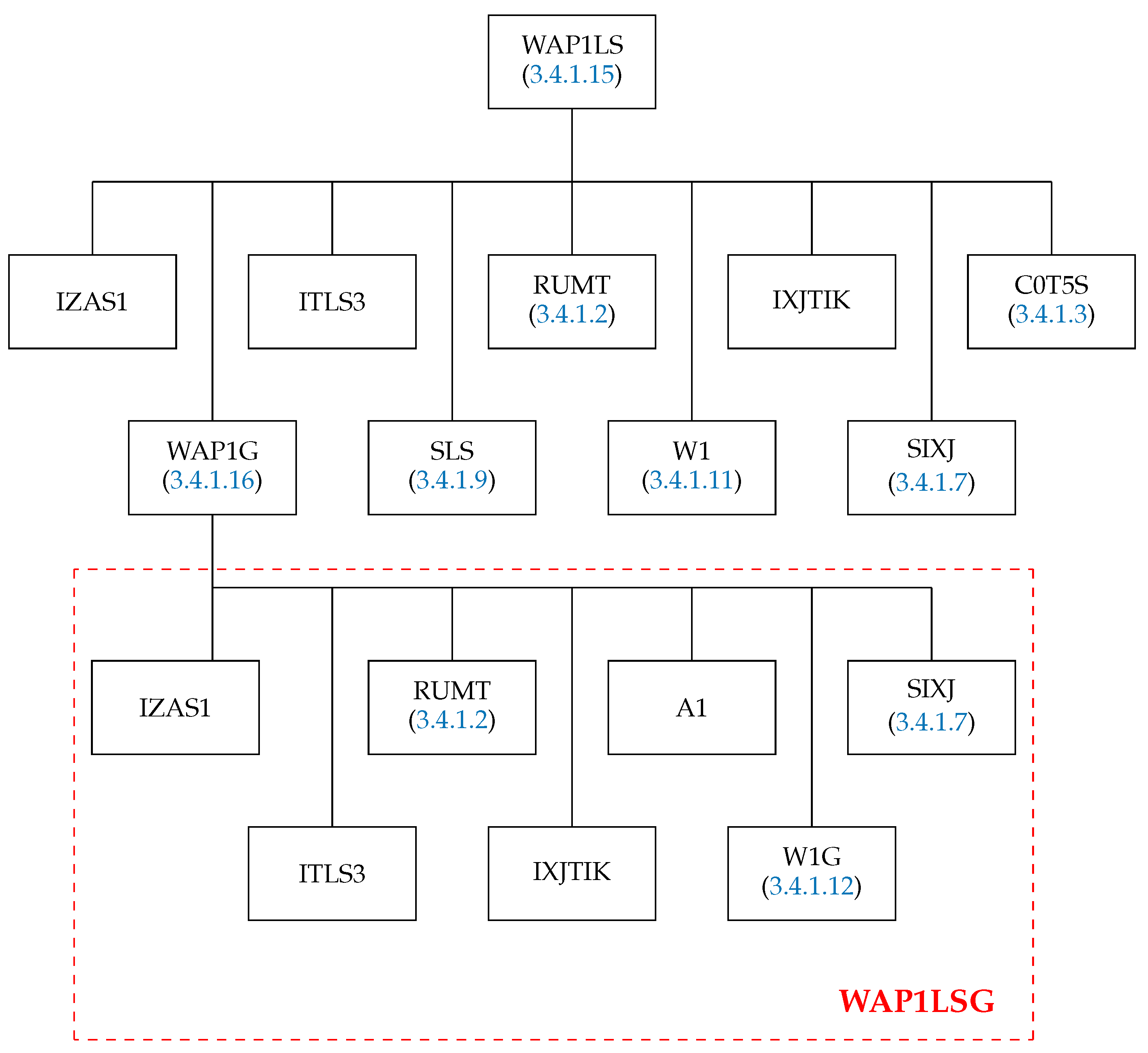
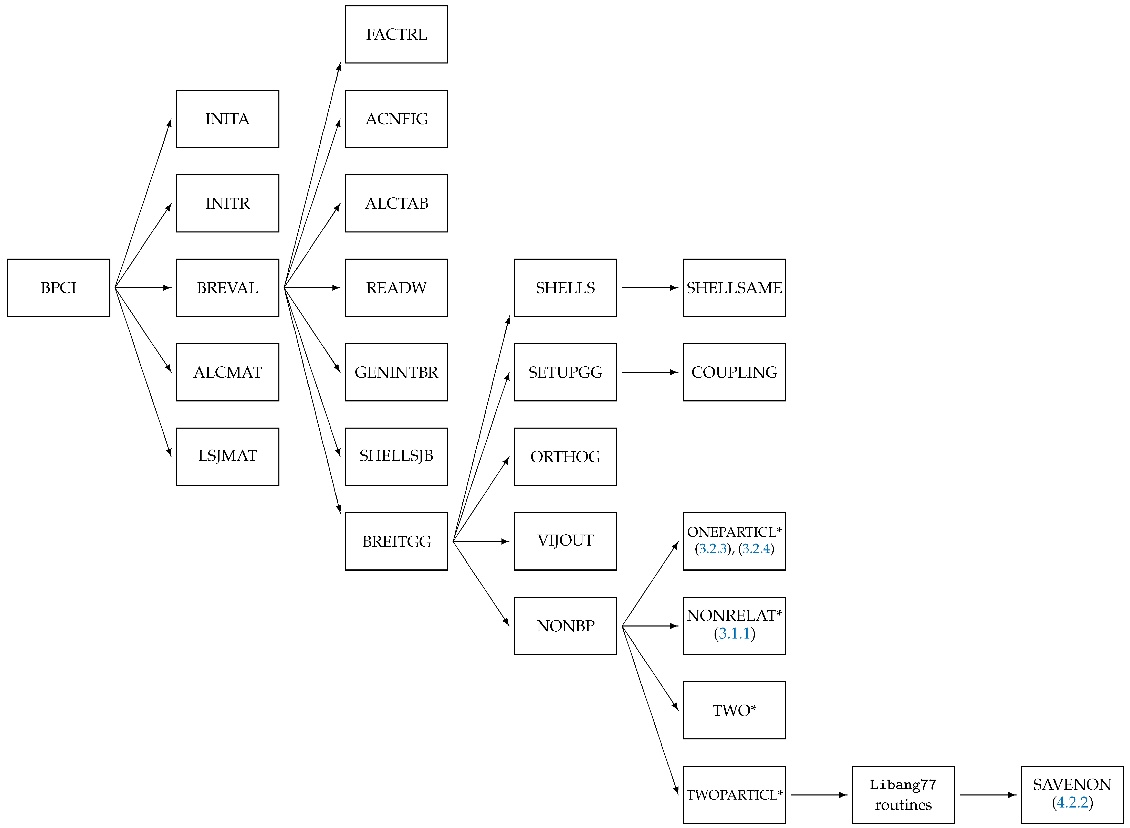
The purpose of NORE and DUDU is to calculate the spin-angular coefficients of the reduced matrix elements of any one- and two-particle operators, following (42) and (64). NORE and DUDU call RECLS and SQLS. The RECLS subroutine group calculates the required recoupling coefficients, and the SQLS subroutine group calculates the standard reduced and completely reduced matrix elements of second quantization operators. NORE calculates the spin-angular coefficients for the Coulomb (24) and orbit–orbit (29) interactions, and DUDU calculates the spin-angular coefficients for fine-structure part (30) of the Breit–Pauli operators. libang77 can be easily used and extended in case we need to calculate the spin-angular coefficients for the second-order effective operator in perturbation theory [82,83,84] (similarly to the relativistic case for RSMBPT [85,86,87,88]) or for any three-particle operator (similarly to the relativistic case for RSMBPT [89,90,91]). All subroutines use the Fano-Racah phase convention [27], as does the Atsp2K software package [20]. It is assumed that all selection rules for the first group of angular momentum (see Table 1, Table 2 and Table 3) are checked before calling this library.

The program library uses completely reduced matrix elements (14) of the operator of second quantization $a^{\left(qls\right)}$ instead of coefficients of the fractional parentage. All completely reduced matrix elements of tensorial operator $a^{\left(qls\right)}$ and all completely reduced matrix elements of the tensorial operator ${\left[a^{\left(qls\right)}\times a^{\left(qls\right)}\right]}^{\left(k_1{k}_2{k}_3\right)}$ [22] required by SQLS are stored in memory. The former is extracted from memory by subroutine SLS (see Section 3.4.1.9), and the latter is extracted from memory by subroutine RWLS (see Section 3.4.1.10). The subroutine SLS that finds RCFP values replace the CFPP and CFPD subroutines from [92], which calculate CFP and were implemented in previous versions of the Atsp software package [1,4,5,6].

3.1. The NORE Subroutine Group

The subroutines from this subroutine group is for calculating the spin-angular parts of reduced matrix elements for a scalar two-particle operator. It contains 18 subroutines. The calculations are performed according to the methodology in P2 [9]. The references in this table also correspond to the numbering of the expressions in P2. Most of the subroutines from this group use COMMON blocks /CONSTS/, /DIAGNL/, and /MEDEFN/ from Atsp2K [20].

3.1.1. The Subroutine NONRELAT*

In

Table 4. Scheme of the expressions for reduced matrix elements of two-particle scalar operators (such as Coulomb or orbit–orbit interactions).

Dis.	$\widehat{\mathit{G}}$	$\widehat{\mathit{G}}\left(\mathit{T}\right)$	$\mathit{\alpha }$	$\mathit{\beta }$	$\mathit{\gamma }$	$\mathit{\delta }$	$\tilde{\mathbf{\Theta }}$	R	$\mathbf{\Delta }$
NONRELAT1
$\alpha \alpha \alpha \alpha$	(47)	(5)	(38), (35)	–	–	–	(48), (49)	(18)	(41)
$\alpha \beta \alpha \beta$	(50)	(6)	(35)	(35)	–	–	(51)	(22)	(41)
$\beta \alpha \beta \alpha$	(50)	(6)	(35)	(35)	–	–	(51)	(22)	(41)
$\alpha \beta \beta \alpha$	(54)	(6)	(35)	(35)	–	–	(55)	(22)	(41)
$\beta \alpha \alpha \beta$	(54)	(6)	(35)	(35)	–	–	(55)	(22)	(41)
NONRELAT2
$\alpha \alpha \beta \beta$	(52)	(6)	(35)	(35)	–	–	(53)	(22)	(41)
NONRELAT31
$\beta \alpha \alpha \alpha$	(56)	(6)	(36)	(34)	–	–	(58)	(22)	(42)
$\alpha \beta \alpha \alpha$	(56)	(6)	(36)	(34)	–	–	(59)	(22)	(42)
NONRELAT32
$\beta \beta \beta \alpha$	(60)	(6)	(34)	(37)	–	–	(62)	(22)	(42)
$\beta \beta \alpha \beta$	(60)	(6)	(34)	(37)	–	–	(63)	(22)	(42)
NONRELAT33
$\beta \gamma \alpha \gamma$	(50)	(7)	(34)	(34)	(35)	–	(51)	(26)	(42)
$\gamma \beta \gamma \alpha$	(50)	(7)	(34)	(34)	(35)	–	(51)	(26)	(42)
$\gamma \beta \alpha \gamma$	(54)	(7)	(34)	(34)	(35)	–	(55)	(26)	(42)
$\beta \gamma \gamma \alpha$	(54)	(7)	(34)	(34)	(35)	–	(55)	(26)	(42)
NONRELAT41
$\gamma \gamma \alpha \beta$	(52)	(7)	(34)	(34)	(35)	–	(53)	(26)	(42)
$\gamma \gamma \beta \alpha$	(52)	(7)	(34)	(34)	(35)	–	(53)	(26)	(42)
$\alpha \beta \gamma \gamma$	(52)	(7)	(34)	(34)	(35)	–	(53)	(26)	(42)
$\beta \alpha \gamma \gamma$	(52)	(7)	(34)	(34)	(35)	–	(53)	(26)	(42)
NONRELAT51
$\alpha \beta \gamma \delta$	(52)	(8)	(34)	(34)	(34)	(34)	(53)	(33)	(43)
$\beta \alpha \gamma \delta$	(52)	(8)	(34)	(34)	(34)	(34)	(53)	(33)	(43)
$\alpha \beta \delta \gamma$	(52)	(8)	(34)	(34)	(34)	(34)	(53)	(33)	(43)
$\beta \alpha \delta \gamma$	(52)	(8)	(34)	(34)	(34)	(34)	(53)	(33)	(43)
$\gamma \delta \alpha \beta$	(52)	(8)	(34)	(34)	(34)	(34)	(53)	(33)	(43)
$\gamma \delta \beta \alpha$	(52)	(8)	(34)	(34)	(34)	(34)	(53)	(33)	(43)
$\delta \gamma \alpha \beta$	(52)	(8)	(34)	(34)	(34)	(34)	(53)	(33)	(43)
$\delta \gamma \beta \alpha$	(52)	(8)	(34)	(34)	(34)	(34)	(53)	(33)	(43)
NONRELAT52
$\alpha \gamma \beta \delta$	(50)	(8)	(34)	(34)	(34)	(34)	(51)	(33)	(43)
$\alpha \gamma \delta \beta$	(54)	(8)	(34)	(34)	(34)	(34)	(55)	(33)	(43)
$\gamma \alpha \delta \beta$	(50)	(8)	(34)	(34)	(34)	(34)	(51)	(33)	(43)
$\gamma \alpha \beta \delta$	(54)	(8)	(34)	(34)	(34)	(34)	(55)	(33)	(43)
$\beta \delta \alpha \gamma$	(50)	(8)	(34)	(34)	(34)	(34)	(51)	(33)	(43)
$\delta \beta \gamma \alpha$	(50)	(8)	(34)	(34)	(34)	(34)	(51)	(33)	(43)
$\beta \delta \gamma \alpha$	(54)	(8)	(34)	(34)	(34)	(34)	(55)	(33)	(43)
$\delta \beta \alpha \gamma$	(54)	(8)	(34)	(34)	(34)	(34)	(55)	(33)	(43)
NONRELAT53
$\alpha \delta \beta \gamma$	(50)	(8)	(34)	(34)	(34)	(34)	(51)	(33)	(43)
$\delta \alpha \gamma \beta$	(50)	(8)	(34)	(34)	(34)	(34)	(51)	(33)	(43)
$\alpha \delta \gamma \beta$	(54)	(8)	(34)	(34)	(34)	(34)	(55)	(33)	(43)
$\delta \alpha \beta \gamma$	(54)	(8)	(34)	(34)	(34)	(34)	(55)	(33)	(43)
$\beta \gamma \alpha \delta$	(50)	(8)	(34)	(34)	(34)	(34)	(51)	(33)	(43)
$\gamma \beta \delta \alpha$	(50)	(8)	(34)	(34)	(34)	(34)	(51)	(33)	(43)
$\beta \gamma \delta \alpha$	(54)	(8)	(34)	(34)	(34)	(34)	(55)	(33)	(43)
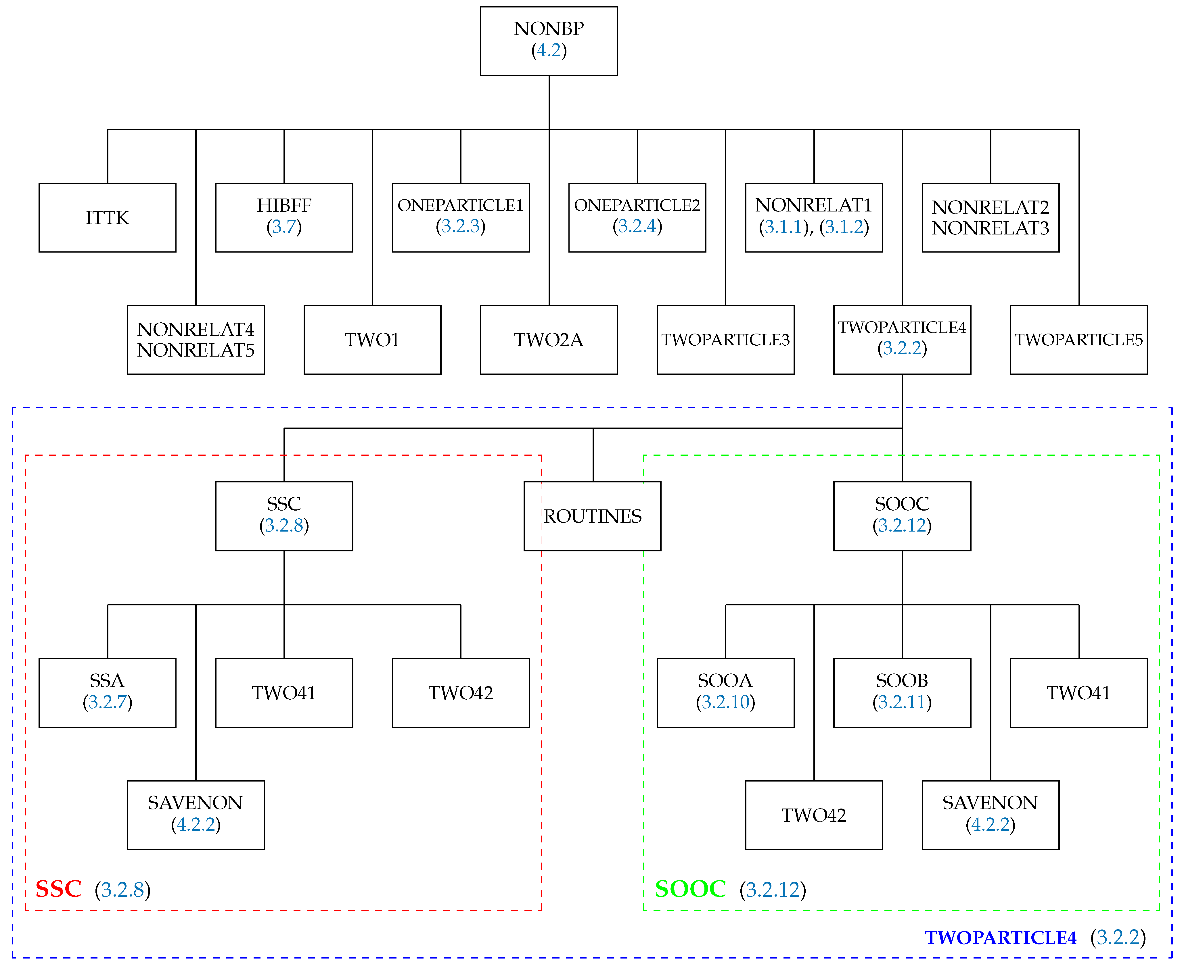
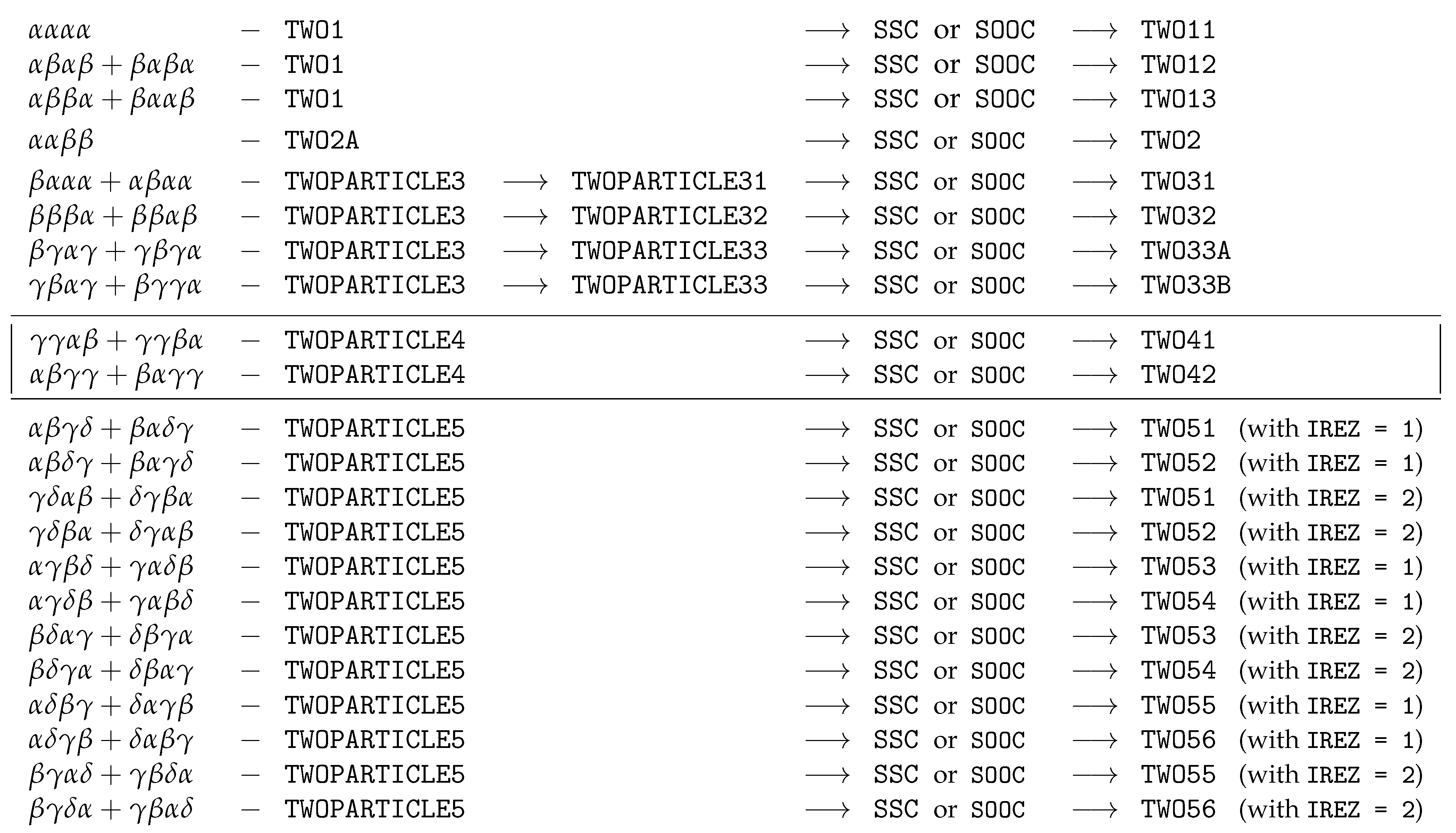
$\gamma \beta \alpha \delta$	(54)	(8)	(34)	(34)	(34)	(34)	(55)	(33)	(43)

, information related to what expressions the subroutines NONRELAT1, NONRELAT2, NONRELAT31, NONRELAT32, NONRELAT33, NONRELAT41, NONRELAT51, NONRELAT52, NONRELAT53 use is presented. The numbering of expressions is the same as in P2, where all these expressions are presented. The call to all these subroutines is from the subroutine NONRELAT. These subroutines calculate spin-angular coefficients for the reduced matrix elements of $\mathcal{T}$ (22) and $\mathcal{U}$ (23), $\mathcal{V}$ (24), and/or ${\mathcal{H}}_{OO}$ (29) operators for all possible distributions from Table 4. As the structure of all the subroutines mentioned earlier is almost the same, only different expressions are used, and different subroutines are called, we will discuss in more detail only one of these subroutines bellow. The subroutines NONRELAT1, NONRELAT2, NONRELAT3, NONRELAT31, NONRELAT32, NONRELAT33, NONRELAT4, NONRELAT41, NONRELAT5, NONRELAT51, NONRELAT52, and NONRELAT53 have counterparts EL1, EL2, EL3, EL31, EL32, EL33, EL4, EL41, EL5, EL51, EL52, and EL53 in the librang90 library [21], respectively. I would also like to point out that the calculation of the one-particle scalar operator $\mathcal{T}$ (22) is integrated into the subroutines NONRELAT1 and NONRELAT31. The SAVENON subroutine (see Section 4.1) with argument value I = 4 returns the calculated spin-angular part of this operator to the program. This makes the calculations themselves more efficient in terms of computing time.

Similar to electrostatic (Coulomb) electron interaction (71) or orbit–orbit interaction (74), the libang77 library can be extended with other two-particle operators that are scalar in l and s spaces. This requires (i) knowledge of the tensorial structure of the intermediate ranks of the operator to be included in the calculations in its irreducible tonsorial form; (ii) programming the corresponding summation of these ranks in the NONRELAT1, NONRELAT2, NONRELAT31, NONRELAT32, NONRELAT33, NONRELAT41, NONRELAT51, NONRELAT52, and NONRELAT53 subroutines, if needed; and (iii) writing new subroutines, similar to COULOMBLS (Section 3.1.3) and ORBITORBIT (Section 3.1.4), for Coulomb and orbit–orbit interactions, which would calculate the two-particle reduced matrix element for the desired operator to be included in the calculations. It is also necessary to maintain the order of subroutine NONRELAT1 (see Section 3.1.2), NONRELAT2, NONRELAT3, NONRELAT31, NONRELAT32, NONRELAT33, NONRELAT4, NONRELAT41, NONRELAT5, NONRELAT51, NONRELAT52, and NONRELAT53, calls similar to those of Coulomb or orbit–orbit interactions.

3.1.2. The Subroutine NONRELAT1

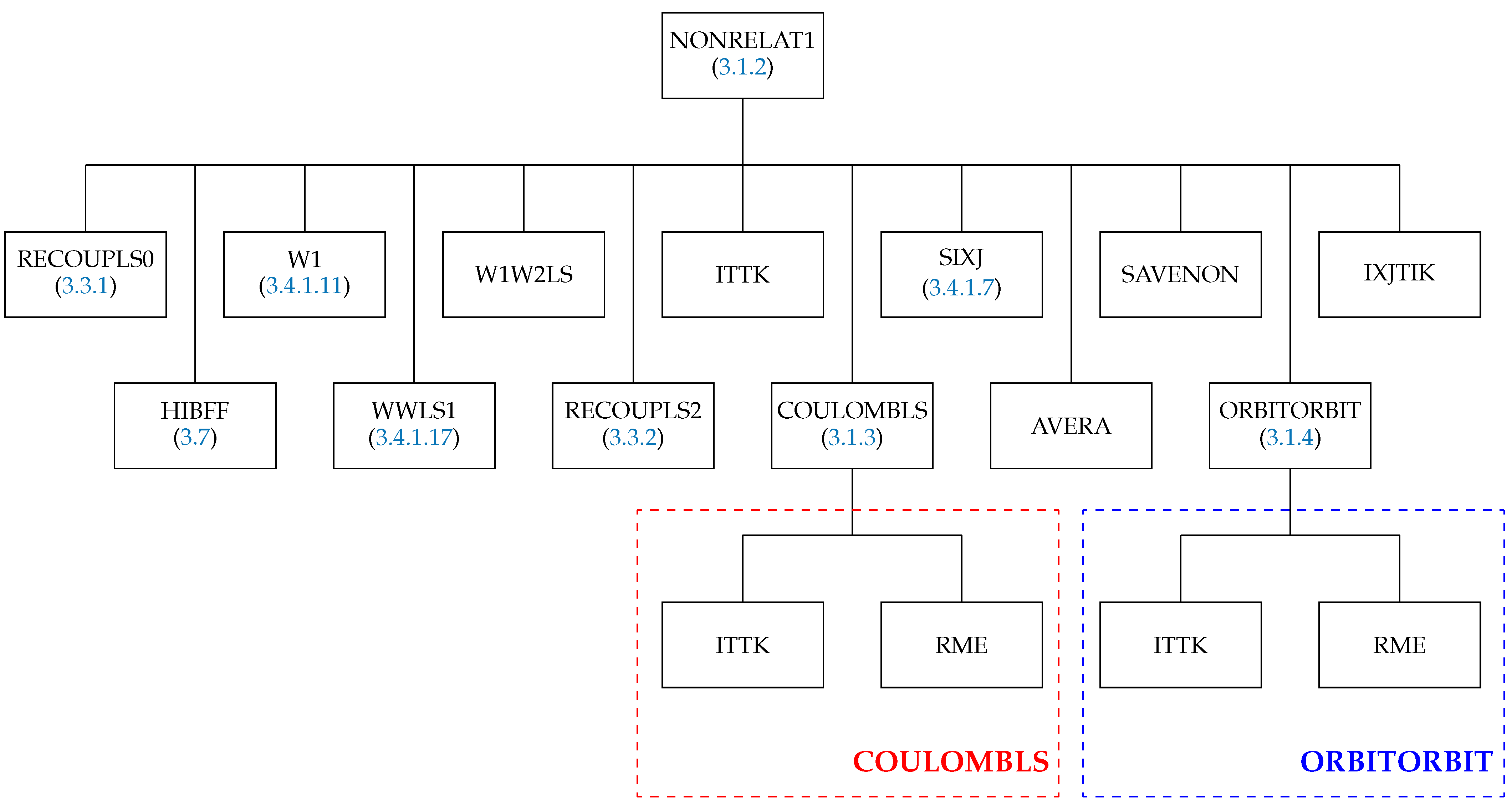
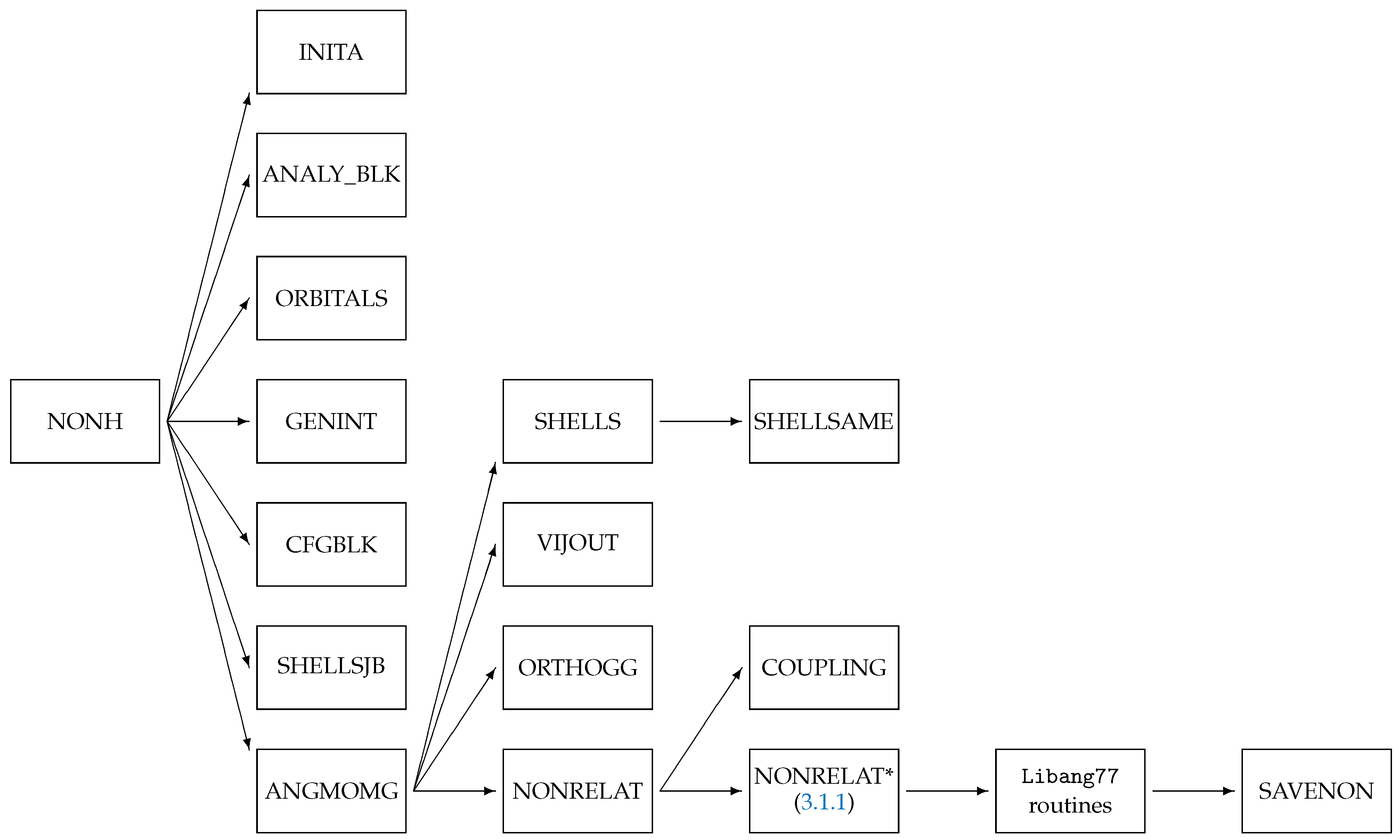
This subroutine calculates spin-angular coefficients for the reduced matrix elements of $\mathcal{V}$ (24) and/or ${\mathcal{H}}_{OO}$ (29) operators for the distributions $\alpha \alpha \alpha \alpha$, $\alpha \beta \alpha \beta$, $\beta \alpha \beta \alpha$, $\alpha \beta \beta \alpha$, and $\beta \alpha \alpha \beta$. This subroutine also calculates spin-angular coefficient of diagonal reduced matrix elements for T (22) and U (23) operators. The structure of this subroutine is presented in Figure 1. First, the subroutine RECOUPLS0 checks the selection rules for the recoupling coefficient. If it is non-zero, then the subroutine HIBFF transfers all necessary variables describing characteristics of interacting shells for calculation from the Atsp2K [20] COMMON block /MEDEFN/ to the arrays placed in COMMON blocks /TRK/ and /TRK2/ (see Section 3.6 and Section 3.7).

In the $\alpha \alpha \alpha \alpha$ case, the subroutine uses expression (5) from P2. In this case,

$$\begin{array}{c}\hfill {\displaystyle \widehat{G}\left(I\right)\sim \sum _{\begin{array}{c}\hfill {\kappa }_{12},{\sigma }_{12}\\ \hfill {\kappa }_{12}^{\prime },{\sigma }_{12}^{\prime }\end{array}}\sum _p\left[{\mathsf{\Theta }}_{IIa}\left(n\lambda ,\mathsf{\Xi }\right)A_a^{\left(00\right)}\left(n\lambda ,\mathsf{\Xi }\right)+{\mathsf{\Theta }}_{IIb}\left(n\lambda ,\mathsf{\Xi }\right)A_{\left(b\right)p,-p}^{\left(kk\right)}\left(n\lambda ,\mathsf{\Xi }\right)\right];}\end{array}$$

(100)

where

$$\begin{array}{c}\hfill A_a^{\left(00\right)}\left(n\lambda ,\mathsf{\Xi }\right)={\left[{\left[a^{\left(l_{\alpha }s\right)}\times {\tilde{a}}^{\left(l_{\alpha }s\right)}\right]}^{\left({\kappa }_1{\sigma }_1\right)}\times {\left[{\tilde{a}}^{\left(l_{\alpha }s\right)}\times a^{\left(l_{\alpha }s\right)}\right]}^{\left({\kappa }_2{\sigma }_2\right)}\right]}^{\left(00\right)}\end{array}$$

(101)

$$\begin{array}{c}\hfill A_{\left(b\right)p,-p}^{\left(kk\right)}\left(n\lambda ,\mathsf{\Xi }\right)={\left[a^{\left(l_{\alpha }s\right)}\times {\tilde{a}}^{\left(l_{\alpha }s\right)}\right]}_{p,-p}^{\left(kk\right)},\end{array}$$

(102)

and

$$\begin{array}{c}\hfill {\mathsf{\Theta }}_{IIa}\left(n\lambda ,\mathsf{\Xi }\right)={\tilde{\mathsf{\Theta }}}_{IIa}\left(n_{\alpha }{\lambda }_{\alpha },n_{\alpha }{\lambda }_{\alpha },n_{\alpha }{\lambda }_{\alpha },n_{\alpha }{\lambda }_{\alpha },\mathsf{\Xi }\right)\\ \hfill ={\displaystyle \frac{1}{2}}{\left(-1\right)}^{k-p}{\left[{\kappa }_1,{\sigma }_1,{\kappa }_2,{\sigma }_2\right]}^{-1/2}\times \left(n_{\alpha }{\lambda }_{\alpha }{n}_{\alpha }{\lambda }_{\alpha }\left|\right|g^{\left({\kappa }_1{\kappa }_{2}k,{\sigma }_1{\sigma }_{2}k\right)}\left|\right|n_{\alpha }{\lambda }_{\alpha }{n}_{\alpha }{\lambda }_{\alpha }\right)\end{array}$$

(103)

and

$$\begin{array}{c}\hfill {\mathsf{\Theta }}_{IIb}\left(n\lambda ,\mathsf{\Xi }\right)={\tilde{\mathsf{\Theta }}}_{IIb}\left(n_{\alpha }{\lambda }_{\alpha },n_{\alpha }{\lambda }_{\alpha },n_{\alpha }{\lambda }_{\alpha },n_{\alpha }{\lambda }_{\alpha },\mathsf{\Xi }\right)\\ \hfill ={\left(-1\right)}^{k-p+1}\left(n_{\alpha }{\lambda }_{\alpha }{n}_{\alpha }{\lambda }_{\alpha }\left|\right|g^{\left({\kappa }_1{\kappa }_{2}k,{\sigma }_1{\sigma }_{2}k\right)}\left|\right|n_{\alpha }{\lambda }_{\alpha }{n}_{\alpha }{\lambda }_{\alpha }\right)\left\{\begin{array}{ccc}{\kappa }_1& {\kappa }_2& k\\ l_{\alpha }& l_{\alpha }& l_{\alpha }\end{array}\right\}\left\{\begin{array}{ccc}{\sigma }_1& {\sigma }_2& k\\ s& s& s\end{array}\right\}.\end{array}$$

(104)

The value of the reduced matrix element of operator (101) is found by subroutine WWLS1 (see Section 3.4.1.17) and that of (102) W1 (see Section 3.4.1.11). The value of coefficient ${\mathsf{\Theta }}_{IIa}\left(n\lambda ,\mathsf{\Xi }\right)$ is calculated by COULOMBLS (see the red frame COULOMBLS in Figure 1 and its detailed description in Section 3.1.3) and/or ORBITORBIT (see the blue frame ORBITORBIT in Figure 1 and its detailed description in Section 3.1.4) subroutines because this coefficient, to the accuracy of a factor and a phase, is equal to that part of the two-electron reduced matrix elements of electrostatic interaction which this subroutine is calculating. The coefficient ${\mathsf{\Theta }}_{IIb}\left(n\lambda ,\mathsf{\Xi }\right)$ is found by COULOMBLS and/or ORBITORBIT and SIXJ (see Section 3.4.1.7), and the recoupling matrix is investigated by RECOUPLS0 (see Section 3.3.1).

For the distributions $\alpha \beta \alpha \beta$ and $\beta \alpha \beta \alpha$, the subroutine NONRELAT1 uses (6) of P2, keeping in mind that $\mathsf{\Theta }\left(n_{\alpha }{\lambda }_{\alpha },n_{\beta }{\lambda }_{\beta },\mathsf{\Xi }\right)$ is expressed as (51) of P2 and tensorial parts $B^{\left({\kappa }_{12}{\sigma }_{12}\right)}\left(n_{\alpha }{\lambda }_{\alpha },\mathsf{\Xi }\right)$, $C^{\left({\kappa }_{12}^{\prime }{\sigma }_{12}^{\prime }\right)}\left(n_{\beta }{\lambda }_{\beta },\mathsf{\Xi }\right)$ are equal to (35) from P2. The coefficients $\mathsf{\Theta }\left(n_{\alpha }{\lambda }_{\alpha },n_{\beta }{\lambda }_{\beta },\mathsf{\Xi }\right)$ are investigated by COULOMBLS and/or ORBITORBIT, the coefficients $B^{\left({\kappa }_{12}{\sigma }_{12}\right)}\left(n_{\alpha }{\lambda }_{\alpha },\mathsf{\Xi }\right)$ and $C^{\left({\kappa }_{12}^{\prime }{\sigma }_{12}^{\prime }\right)}\left(n_{\beta }{\lambda }_{\beta },\mathsf{\Xi }\right)$ are found by W1W2LS from the SQLS1 module, and the recoupling matrix is calculated by RECOUPLS2 from Section 3.3.2.

For the distributions $\alpha \beta \beta \alpha$ and $\beta \alpha \alpha \beta$, the subroutine NONRELAT1 uses (6) of P2, keeping in mind that $\mathsf{\Theta }\left(n_{\alpha }{\lambda }_{\alpha },n_{\beta }{\lambda }_{\beta },\mathsf{\Xi }\right)$ is expressed as (55) in P2 and tensorial parts $B^{\left({\kappa }_{12}{\sigma }_{12}\right)}\left(n_{\alpha }{\lambda }_{\alpha },\mathsf{\Xi }\right)$ and $C^{\left({\kappa }_{12}^{\prime }{\sigma }_{12}^{\prime }\right)}\left(n_{\beta }{\lambda }_{\beta },\mathsf{\Xi }\right)$ are equal to (35) from P2. The coefficients $\mathsf{\Theta }\left(n_{\alpha }{\lambda }_{\alpha },n_{\beta }{\lambda }_{\beta },\mathsf{\Xi }\right)$ are investigated by COULOMBLS and/or ORBITORBIT and SIXJ, the coefficients $B^{\left({\kappa }_{12}{\sigma }_{12}\right)}\left(n_{\alpha }{\lambda }_{\alpha },\mathsf{\Xi }\right)$ and $C^{\left({\kappa }_{12}^{\prime }{\sigma }_{12}^{\prime }\right)}\left(n_{\beta }{\lambda }_{\beta },\mathsf{\Xi }\right)$ are found by W1W2LS from the SQLS1 library, and the recoupling matrix is calculated by RECOUPLS2.

The subroutine has the following arguments:

1.

IA and IB in the arrays LJ, NJ, LJ, NOSH1, NOSH2, J1QN1, J1QN2, and IJFUL from the COMMON block /MEDEFN/ point to the position of the two interacting shells.

2.

IIRE must be set equal to $\left\{\begin{array}{cc}\mathtt{0}\hfill & \mathrm{when}\mathrm{the}\mathrm{reduced}\mathrm{matrix}\mathrm{element}\mathrm{is}\mathrm{diagonal},\hfill \\ \mathtt{1}\hfill & \mathrm{when}\mathrm{the}\mathrm{reduced}\mathrm{matrix}\mathrm{element}\mathrm{is}\mathrm{off}-\mathrm{diagonal}\hfill \end{array}\right.$ with respect to configuration state functions.

Additionally, the subroutine uses COMMON block /OPERAT/ ICOLOM,ISOTOP,IORBORB. If ICOLOM≠0, then the program calculates the Coulomb interaction, and if IORBORB≠0, the programs calculates the orbit–orbit interaction. Both of these parameters can be immediately non-zero.

3.1.3. The Subroutines COULOMBLS

This subroutine calculates the two-electron reduced matrix elements (72) of electrostatic interaction

$$\left(n_i{\lambda }_i{n}_j{\lambda }_j∥g_{Coulomb}^{\left(kk0,000\right)}∥n_i^{\prime }{\lambda }_i^{\prime }{n}_j^{\prime }{\lambda }_j^{\prime }\right),$$

according to formula (9) of P1. The values of these two-electron reduced matrix elements are needed because of (see P2)

$$\begin{array}{c}\hfill \mathsf{\Theta }\left(\mathsf{\Xi }\right)\sim \left(n_i{\lambda }_i{n}_j{\lambda }_j∥g∥n_{i^{\prime }}{\lambda }_{i^{\prime }}{n}_{j^{\prime }}{\lambda }_{j^{\prime }}\right).\end{array}$$

(105)

The structure of the subroutine COULOMBLS is given in the red frame labelled COULOMBLS in Figure 1. This subroutine has the counterpart subroutine COULOM in the relativistic spin-angular integration library librang90 [21].

The subroutine has the following arguments:

1.

L1 is the orbital quantum number $l_i$.

2.

L2 is the orbital quantum number $l_j$.

3.

L3 is the orbital quantum number $l_i^{\prime }$.

4.

L4 is the orbital quantum number $l_j^{\prime }$.

5.

KL is the rank k of the operator $g_{Coulomb}^{\left(kk0,000\right)}$.

6.

AA is the value of the two-electron reduced matrix element (72) which is returned by the subroutine.

The value of the output argument AA of this subroutine is

$$\begin{array}{c}\hfill \mathtt{A}\mathtt{A}=2{\left[k\right]}^{1/2}\left(l_i∥C^{\left(k\right)}∥l_i^{\prime }\right)\left(l_j∥C^{\left(k\right)}∥l_j^{\prime }\right).\end{array}$$

(106)

3.1.4. The Subroutine ORBITORBIT

This subroutine calculates the two-electron reduced matrix elements (82) of orbit–orbit interaction

$$\begin{array}{c}\hfill \left(n_i{\lambda }_i{n}_j{\lambda }_j∥H_{oo3}^{(kk0,000)}∥n_{i^{\prime }}{\lambda }_{i^{\prime }}{n}_{j^{\prime }}{\lambda }_{j^{\prime }}\right).\end{array}$$

The values of these two-electron reduced matrix elements are needed because of (see P2)

$$\begin{array}{c}\hfill \mathsf{\Theta }\left(\mathsf{\Xi }\right)\sim \left(n_i{\lambda }_i{n}_j{\lambda }_j∥g∥n_{i^{\prime }}{\lambda }_{i^{\prime }}{n}_{j^{\prime }}{\lambda }_{j^{\prime }}\right).\end{array}$$

(107)

The value of the output argument AA of this subroutine is the two-electron reduced matrix element (82) of orbit–orbit term $H_{oo3}^{(kk0,000)}$. The structure of the subroutine ORBITORBIT is given in the blue frame labelled ORBITORBIT in Figure 1.

The subroutine has the following arguments:

1.

L1 is the orbital quantum number $l_i$.

2.

L2 is the orbital quantum number $l_j$.

3.

L3 is the orbital quantum number $l_i^{\prime }$.

4.

L4 is the orbital quantum number $l_j^{\prime }$.

5.

KL is the rank k of the operator $H_{oo3}^{(kk0,000)}$.

6.

AA is the value of the two-electron reduced matrix element (82) which is returned by the subroutine.

3.2. The DUDU Subroutine Group

The subroutines from this subroutine group serve to calculate the spin-angular parts of reduced matrix elements of any one- or two-particle Breit–Pauli operators, where in the most general case, the final ranks k and k in the spaces l and s (see (64)) are not equal to zero. It contains 44 subroutines. Most of the subroutines from this module use regular COMMON blocks CONSTS and MEDEFN from the Atsp2K package [20]. Similar to the NORE subroutine group, it uses the methodology described in P2 and P8. Therefore, the arrangement of the subroutines from the DUDU group is analogous to that of the NORE group. This subroutine group can easily be extended with any other one- or two-particle operators.

In fact, most of the subroutines in this group are designed to calculate the spin-angular coefficients of Breit-Paul two-particle operators. These are the most complex physical operators; their calculation is the most complicated, and this is the most complicated part of the libang77 library. To make it easier to understand how the subroutines in this group are linked and function, we present the Bpci program scheme in Figure 2, which shows how the subroutine NONBP organizes the calculation of the spin-angular part of two-particle Breit-Paul operators (for more details about the program Bpci and its subroutine NONBP, see Section 4.2). Before performing calculations, NONBP checks some triangular deltas (subprogram ITTK) and, if they are not equal to zero, subprogram HIBFF fills in the corresponding arrays required using the libang77 library, as there is an interface between Atsp2K [20] and the libang77 library (see Section 3.7). Next, depending on the operator under consideration, the subroutine NONBP calls the subroutine ONEPARTICLE1 or ONEPARTICLE1 in the case of a one-particle operator; in the case of a two-particle scalar operator (in l and s spaces), it calls one of the subroutines NONRELAT1, NONRELAT2, NONRELAT3, NONRELAT4, or NONRELAT5; and in the case of a two-particle non-scalar operator (in l and s spaces), it calls one of the subroutines TWO1, TWO2A, TWOPARTICLE3, TWOPARTICLE4, or TWOPARTICLE5. Each of these subroutines is represented by a separate square in Figure 2, except for NONRELAT2, NONRELAT3, NONRELAT4, and NONRELAT5, which are not represented by four separate blocks but are combined into two separate squares. These subroutines NONRELAT* belong to the program group NORE (see Section 3.1) and have already been described in Section 3.1.1 and Section 3.1.2. Now, we will examine the essential subroutines of the DUDU group separately.

3.2.1. The Subroutines TWO1, TWO2A, and TWOPARTICLE*

For subroutines TWO1, TWO2A,TWOPARTICLE3, TWOPARTICLE4, and TWOPARTICLE5, similar to subroutines NONRELAT1, NONRELAT2, NONRELAT31, NONRELAT32, NONRELAT33, NONRELAT41, NONRELAT51, NONRELAT52, NONRELAT53 in Section 3.1.1 and Table 4, the information in Figure 3 shows which distribution is analyzed by which subroutine, where the distribution is in the first column and the name of the subroutine is in the second column. I also point out that subroutines TWO1, TWO2A,TWOPARTICLE3, and TWOPARTICLE4 use expressions from P2 (with improvements presented in P8), while subroutine TWOPARTICLE5 uses expressions from P8.

The call to all these subroutines is from the subroutine NONBP (see Figure 2). The following columns (from the third to the fifth) in Figure 3 show the further sequence of calculating the spin-angular coefficients. The fourth column indicates which subroutines calculate the two-particle reduced matrix elements of the physical operator for a specific distribution. Since there are only two physical operators among the Breit–Pauli operators that are two-particle and non-scalar in either the l or s spaces, their calculation is performed by only two different subroutines. The SSC subroutine (see Section 3.2.8) calculates the reduced matrix element of spin–spin interaction, while the SOOC subroutine (see Section 3.2.12) calculates the reduced matrix element of spin–other orbit interaction. The remaining subroutines (in the third and fifth columns) perform a certain part of the calculation of the spin-angular coefficients. The calculated values of these coefficients are transferred by the SSC or SOOC subroutine to the SAVENON subroutine (for more details, see Section 4.2.2). As an example, the blue frame TWOPARTICLE4 in Figure 2 illustrates how the calculation scheme is implemented programmatically for the program call sequence defined by the frame in Figure 3 (for more details, see Section 3.2.2).

Similar to spin–spin and spin–other orbit interactions, the libang77 library can be extended with other two-particle operators that are non-scalar in l and s spaces. This requires (i) knowledge of the tensorial structure of the operator to be included in the calculations in its irreducible tonsorial form; (ii) programming the corresponding summation of these ranks in the TWO1, TWO2A, TWOPARTICLE31, TWOPARTICLE32, TWOPARTICLE33, TWOPARTICLE4, and TWOPARTICLE5 subroutines, if needed; (iii) writing the new subroutines, similar to SSC and SOOC, for spin–spin and spin–other orbit interactions, which would calculate the two-particle reduced matrix element for the desired operator to be included in the calculations; and (iv) maintaining the order of subroutine calls specified in Figure 3.

3.2.2. The Subroutine TWOPARTICLE4

This subroutine calculates spin-angular coefficients for the reduced matrix elements of ${\mathcal{H}}_{SS}$ (89) and ${\mathcal{H}}_{SOO}$ (92) operators for the distributions $\gamma \gamma \alpha \beta$, $\gamma \gamma \beta \alpha$, $\alpha \beta \gamma \gamma$, and $\beta \alpha \gamma \gamma$. The structure of the subroutine is presented in the blue frame TWOPARTICLE4 of Figure 2. The block ROUTINES in Figure 2 corresponds to the following subroutines: EILE, HIBFF (see Section 3.7), ITTK, RLSP00 (see Section 3.3.7), ITREXG2, and ITREXG. The subroutine HIBFF transfers all necessary variables describing characteristics of interacting shells for calculation from the Atsp2K [20] COMMON block /MEDEFN/ to the arrays placed in COMMON blocks /TRK/ and /TRK2/ (see Section 3.6 and Section 3.7). The subroutines ITTK and RLSP00 check some selection rules for the recoupling coefficient. If it is non-zero, then the subroutine calls RLSP00 to calculate some part of recoupling coefficient, and SSC or SOOC with the EXTERNAL argument XXX ≡ TWO41 or TWO42 (see Figure 3) are called to calculate the remaining part of spin-angular coefficient.

The subroutine TWOPARTICLE4 has the arguments IA, IB, IC, and ID, which point to the relevant shells in the arrays LJ, NJ, LJ, NOSH1, NOSH2, J1QN1, J1QN2, and IJFUL from the COMMON block /MEDEFN/ of Atsp2K package [20].

3.2.3. The Subroutine ONEPARTICLE1

The purpose of the subroutine ONEPARTICLE1 is to calculate the spin-angular coefficients of the diagonal reduced matrix elements for the one-particle operator with respect to configuration state functions (42). Its structure is presented in Figure 4. First, the subroutines RLSP0 and RLSP1 check the selection rules for the recoupling coefficient. If it is non-zero, then the subroutine RLSP1 computes it (for more details, see Section 3.3.8), but before this, the subroutine W1 computes reduced matrix elements (138) (for more details, see Section 3.4.1.11). Additionally, the subroutine calls an EXTERNAL subroutine XXX whose name XXX is specified in the formal arguments of the subroutine ONEPARTICLE1. The subroutine XXX calculates the reduced matrix element of the desired physical operator. The subroutine HIBFF is the interface between Atsp2K [20] and the SQLS subroutine group.

The subroutine has the following arguments:

1.

K1 is the rank $k_l$ of the operator $F^{\left(k_l{k}_s\right)}$ (see (42)) in l space.

2.

K2 is the rank $k_s$ of the operator $F^{\left(k_l{k}_s\right)}$ (see (42)) in s space.

3.

IA in the arrays LJ, NJ, LJ, NOSH1, NOSH2, J1QN1, J1QN2, and IJFUL from the COMMON block /MEDEFN/ point to the position of the interacting shell.

4.

XXX is the name of the subroutine corresponding to the physical operator for which the subroutine performs the spin-angular integration. The allowed names for this argument are SPINOR (for spin–own orbit interaction (48)), TRANSITION (for transition operators $E^k$ and $M^k$), CONTAC (for Fermi-contact interaction (51)), QDRPOL (for electric quadrupole interaction (54)), ORBIT (for orbit term of hyperfine structure interaction 59)), DIPOL (for spin-dipole term of hyperfine structure interaction (61)), and VOLUM (for electron density at the nucleus).

The output value of the spin-angular part of the reduced matrix element handles the regular subroutine SAVE from Atsp via the subroutine SAVENON.

3.2.4. The Subroutine ONEPARTICLE2

The purpose of the subroutine ONEPARTICLE2 is to calculate the spin-angular coefficients of the off-diagonal reduced matrix elements for the one-particle operator with respect to configuration state functions (42). Its structure is presented in Figure 5. First, the subroutines RLSP0 and RLSP2 check the selection rules for the recoupling coefficient. If it is non-zero, then the subroutine RLSP2 computes it (for more details, see Section 3.3.9), but before this, the subroutine C0T5S generates a Clebsch–Gordan coefficient (for more details, see Section 3.4.1.3) depending on the occupation number of shells, and the subroutine SLS computes the reduced matrix element (136) (see Section 3.4.1.9). Additionally, the subroutine calls an EXTERNAL subroutine XXX whose name XXX is specified in the formal arguments of the subroutine ONEPARTICLE2. The subroutine XXX calculates the reduced matrix element of the desired physical operator. The subroutine HIBFF is the interface between Atsp2K [20] and the SQLS subroutine group.

The subroutine has the following arguments:

1.

K1 is the rank $k_l$ of the operator $F^{\left(k_l{k}_s\right)}$ (see (42)) in l space.

2.

K2 is the rank $k_s$ of the operator $F^{\left(k_l{k}_s\right)}$ (see (42)) in s space.

3.

IIA in the arrays LJ, NJ, LJ, NOSH1, NOSH2, J1QN1, J1QN2, and IJFUL from the COMMON block /MEDEFN/ point to the shell on which the creation operator acts.

4.

IIB in the arrays LJ, NJ, LJ, NOSH1, NOSH2, J1QN1, J1QN2, and IJFUL from the COMMON block /MEDEFN/ point to the shell on which the annihilation operator acts.

5.

XXX is the name of the subroutine corresponding to the physical operator for which the subroutine performs the spin-angular integration. The allowed names for this argument are SPINOR (for spin–own orbit interaction (48)), TRANSITION (for transition operators Ek, and Mk), CONTAC (for Fermi-contact interaction (51)), QDRPOL (for electric quadrupole interaction (54)), ORBIT (for orbit term of hyperfine structure interaction 59)), DIPOL (for spin-dipole term of hyperfine structure interaction (61)), and VOLUM (for electron density at the nucleus).

The output value of the spin-angular part of the reduced matrix element handles the regular subroutine SAVE from Atsp via the subroutine SAVENON.

Similar to spin–own orbit (see Section 3.2.5), E1/E2 transitions (see Section 4.3), or hyperfine structure operators (see Section 4.5), the libang77 library can be extended with other one-particle operators. This requires (i) knowledge of the tensorial structure of the operator to be included in the calculations in its irreducible tensorial form; (ii) writing new subroutines, similar, for example, to SPINOR, for spin–own orbit interactions, which would calculate the one-particle reduced matrix element for the desired operator to be included in the calculations; and (iii) maintaining the order of calls for subroutines ONEPARTICLE1 and ONEPARTICLE2 similar to those of spin–own orbit (see Section 3.2.5), E1/E2 transitions (see Section 4.3), or hyperfine structure operators (see Section 4.5).

3.2.5. The Program Function SPINOR

The program function SPINOR investigates the one-electron reduced matrix elements of the spin–own orbit interaction operator

$$\begin{array}{c}\hfill \left(n_i{\lambda }_i∥f_{s-o}^{\left(11\right)}∥n_j^{\prime }{\lambda }_j^{\prime }\right),\end{array}$$

(108)

according to formula (48).

The subroutine has the following arguments:

1.

L1 is the orbital quantum number l of interacting shell on which the creation operator acts.

2.

L2 is the orbital quantum number l of the interacting shell on which the annihilation operator acts.

3.

I is the output variable that indicates what physical interactions the subroutine has calculated for the one-electron reduced matrix elements. I = 5, in the case of the spin–own orbit interaction operator.

4.

S is the value of the reduced matrix element, which is returned by the subroutine.

It should be noted that instead of the reduced matrix element (48), the program function actually calculates the S value:

$$\begin{array}{c}\hfill \mathtt{S}=-\sqrt{6l\left(l+1\right)\left(2l+1\right)}\delta \left(l,0\right)\sqrt{\left(2L+1\right)\left(2S+1\right)}.\end{array}$$

(109)

This is because the library presented in this paper was created much later than the Atsp package. Therefore, when integrating libang77 into Atsp, efforts were made to maintain the established Atsp structure and change the computer package as little as possible.

Multiplier ${\displaystyle \frac{Z{\alpha }^2}{4}}$ from the reduced matrix element (48) is included via the program function ZETA from regular Atsp library librad, which calculates the radial integral $\left(nl∥{\displaystyle \frac{1}{r^3}}∥nl\right)$. Meanwhile, multiplier $M\left(L,S,k_l,k_s\right)$ for the spin–own orbit interaction operator $M\left(L,S,k_l,k_s\right)\equiv \sqrt{\left(2L+1\right)\left(2S+1\right)}$ from (42) is additionally included in this subroutine.

3.2.6. The Subroutine SS1

The subroutine SS1 investigates the spin–spin operator, which has the tensorial form (89) and finds the sum of two-electron reduced matrix elements (90) and (91)

$$\begin{array}{c}\hfill \left(n_i{\lambda }_i{n}_j{\lambda }_j∥H_{ss}^{\left(k+1k-12,112\right)}∥n_i^{\prime }{\lambda }_i^{\prime }{n}_j^{\prime }{\lambda }_j^{\prime }\right)+\left(n_i{\lambda }_i{n}_j{\lambda }_j∥H_{ss}^{\left(k-1k+12,112\right)}∥n_i^{\prime }{\lambda }_i^{\prime }{n}_j^{\prime }{\lambda }_j^{\prime }\right)\end{array}$$

(110)

for distributions $\alpha \alpha \alpha \alpha$, $\alpha \beta \alpha \beta$, and $\beta \alpha \beta \alpha$ from Table 4.

The subroutine has the following arguments:

1.

L1 is the orbital quantum number l of the first interacting shell ($\alpha$ for distributions $\alpha \alpha \alpha \alpha$ and $\alpha \beta \alpha \beta$ and $\beta$ for distribution $\beta \alpha \beta \alpha$) on which the creation operator acts.

2.

L2 is the orbital quantum number l of the second interacting shell ($\alpha$ for distributions $\alpha \alpha \alpha \alpha$ and $\beta \alpha \beta \alpha$ and $\beta$ for distribution $\alpha \beta \alpha \beta$) on which the creation operator acts.

3.

KL1 is the rank $k+1$ for operator $H_{ss}^{\left(k+1k-12,112\right)}$ or rank $k-1$$H_{ss}^{\left(k-1k+12,112\right)}$.

4.

KL2 is the rank $k-1$ for operator $H_{ss}^{\left(k+1k-12,112\right)}$ or rank $k+1$$H_{ss}^{\left(k-1k+12,112\right)}$.

5.

AA is the value of the sum of the two-electron reduced matrix elements (90) and (91), which is returned by the subroutine.

Additionally, the multiplier $M\left(L,S,k,k\right)$ from (64) for the spin–spin interaction operator $M\left(L,S,k,k\right)\equiv \sqrt{\left(2L+1\right)\left(2S+1\right)}$ is included in the output AA of this subroutine.

3.2.7. The Subroutine SSA

The subroutine SSA investigates the spin–spin operator, which has the tensorial form (89) and finds the sum of two-electron reduced matrix elements (90) and (91)

$$\begin{array}{c}\hfill \left(n_i{\lambda }_i{n}_j{\lambda }_j∥H_{ss}^{\left(k+1k-12,112\right)}∥n_i^{\prime }{\lambda }_i^{\prime }{n}_j^{\prime }{\lambda }_j^{\prime }\right)+\left(n_i{\lambda }_i{n}_j{\lambda }_j∥H_{ss}^{\left(k-1k+12,112\right)}∥n_i^{\prime }{\lambda }_i^{\prime }{n}_j^{\prime }{\lambda }_j^{\prime }\right)\end{array}$$

(111)

for distributions $\alpha \beta \beta \alpha$, $\beta \alpha \alpha \beta$, and $\alpha \alpha \beta \beta$, from Table 4.

The subroutine has the following arguments:

1.

L1 is the orbital quantum number l of the first interacting shell ($\alpha$ for distributions $\alpha \beta \beta \alpha$ and $\alpha \alpha \beta \beta$ and $\beta$ for distribution $\beta \alpha \alpha \beta$) on which the creation operator acts.

2.

L2 is the orbital quantum number l of the second interacting shell ($\alpha$ for distributions $\alpha \alpha \beta \beta$ and $\beta \alpha \alpha \beta$ and $\beta$ for distribution $\alpha \beta \beta \alpha$) on which the creation operator acts.

3.

L3 is the orbital quantum number l of the third interacting shell ($\alpha$ for distribution $\beta \alpha \alpha \beta$ and $\beta$ for distributions $\alpha \beta \beta \alpha$ and $\alpha \alpha \beta \beta$) on which the creation operator acts.

4.

L4 is the orbital quantum number l of the fourth interacting shell ($\alpha$ for distribution $\alpha \beta \beta \alpha$ and $\beta$ for distributions $\alpha \alpha \beta \beta$ and $\beta \alpha \alpha \beta$) on which the creation operator acts.

5.

KL1 is the rank $k+1$ for operator $H_{ss}^{\left(k+1k-12,112\right)}$ or rank $k-1$$H_{ss}^{\left(k-1k+12,112\right)}$.

6.

KL2 is the rank $k-1$ for operator $H_{ss}^{\left(k+1k-12,112\right)}$ or rank $k+1$$H_{ss}^{\left(k-1k+12,112\right)}$.

7.

AA is the value of the sum of the two-electron reduced matrix elements (90) and (91), which is returned by the subroutine.

Additionally, the multiplier $M\left(L,S,k,k\right)$ from (64) for the spin–spin interaction operator $M\left(L,S,k,k\right)\equiv \sqrt{\left(2L+1\right)\left(2S+1\right)}$ is included in the output AA of this subroutine.

3.2.8. The Subroutine SSC

The subroutine SSC investigates the spin–spin operator, which has the tensorial form (89) and finds the sum of two-electron reduced matrix elements (90) and (91)

$$\begin{array}{c}\hfill \left(n_i{\lambda }_i{n}_j{\lambda }_j∥H_{ss}^{\left(k+1k-12,112\right)}∥n_i^{\prime }{\lambda }_i^{\prime }{n}_j^{\prime }{\lambda }_j^{\prime }\right)+\left(n_i{\lambda }_i{n}_j{\lambda }_j∥H_{ss}^{\left(k-1k+12,112\right)}∥n_i^{\prime }{\lambda }_i^{\prime }{n}_j^{\prime }{\lambda }_j^{\prime }\right).\end{array}$$

(112)

This subroutine is used for all distributions (see Table 4) except $\alpha \alpha \alpha \alpha$, $\alpha \beta \alpha \beta$, $\beta \alpha \beta \alpha$, $\alpha \beta \beta \alpha$, $\beta \alpha \alpha \beta$, and $\alpha \alpha \beta \beta$. In the latter cases, instead of the subroutine SSC, the subroutines SS1 (the call is from the subroutines SS1111 and SS1212) and SSA (the call is from the subroutines SS1221, SS1221, and SS1122) are used (see Section 3.2.6 and Section 3.2.7). The structure of the subroutine is presented in the red frame SSC of Figure 2. But, please note that, depending on the distribution, the subroutine calls one of the subroutines TWO41 or TWA41, when the call is made from the subroutine NONRELAT4, as shown in Figure 2. This is done through the EXTERNAL argument XXX. When the call is made from other NONRELAT* group subroutines, other subroutines are specified via the argument. For more details, see the descriptions of the arguments below.

The subroutine has the following arguments:

1.

IG argument is not currently used.

2.

KL is the rank $k+1$ for operator $H_{ss}^{\left(k+1k-12,112\right)}$.

3.

IA points to the first from the left interacting shell on which one of the operators of second quantization acts in the configuration state function in the arrays LJ, NJ, LJ, NOSH1, NOSH2, J1QN1, J1QN2, and IJFUL from the COMMON block /MEDEFN/. For example, we have the following sequence of second quantization operators: $a_4$$a_7$${\tilde{a}}_5$${\tilde{a}}_3$, where the indices of the second quantization operators indicate the shell number in the configuration state function. In this case, the argument is IA=3.

4.

IB points to the second from the left interacting shell on which one of the operators of second quantization acts in the configuration state function in the arrays LJ, NJ, LJ, NOSH1, NOSH2, J1QN1, J1QN2, and IJFUL from the COMMON block /MEDEFN/. For example, we have the following sequence of second quantization operators: $a_4$$a_7$${\tilde{a}}_5$${\tilde{a}}_3$, where the indices of the second quantization operators indicate the shell number in the configuration state function. In this case, the argument is IB = 4.

5.

IC points to the third from the left interacting shell on which one of the operators of second quantization acts in the configuration state function in the arrays LJ, NJ, LJ, NOSH1, NOSH2, J1QN1, J1QN2, and IJFUL from the COMMON block /MEDEFN/. For example, we have the following sequence of second quantization operators: $a_4$$a_7$${\tilde{a}}_5$${\tilde{a}}_3$, where the indices of the second quantization operators indicate the shell number in the configuration state function. In this case, the argument is IC = 5.

6.

ID points to the fourth from the left interacting shell on which one of the operators of second quantization acts in the configuration state function in the arrays LJ, NJ, LJ, NOSH1, NOSH2, J1QN1, J1QN2, and IJFUL from the COMMON block /MEDEFN/. For example, we have the following sequence of second quantization operators: $a_4$$a_7$${\tilde{a}}_5$${\tilde{a}}_3$, where the indices of the second quantization operators indicate the shell number in the configuration state function. In this case, the argument is ID = 7.

7.

IIA points to the shell on which the first operator of the second quantization acts in the arrays LJ, NJ, LJ, NOSH1, NOSH2, J1QN1, J1QN2, and IJFUL from the COMMON block /MEDEFN/. For example, for the distribution $\alpha \beta \gamma \delta$, the shell is $\alpha$.

8.

IIB points to the shell on which the second operator of the second quantization acts in the arrays LJ, NJ, LJ, NOSH1, NOSH2, J1QN1, J1QN2, and IJFUL from the COMMON block /MEDEFN/. For example, for the distribution $\alpha \beta \gamma \delta$, the shell is $\beta$.

9.

IIC points to the shell on which the third operator of the second quantization acts in the arrays LJ, NJ, LJ, NOSH1, NOSH2, J1QN1, J1QN2, and IJFUL from the COMMON block /MEDEFN/. For example, for the distribution $\alpha \beta \gamma \delta$, the shell is $\gamma$.

10.

IID points to the shell on which the fourth operator of the second quantization acts in the arrays LJ, NJ, LJ, NOSH1, NOSH2, J1QN1, J1QN2, and IJFUL from the COMMON block /MEDEFN/. For example, for the distribution $\alpha \beta \gamma \delta$, the shell is $\delta$.

11.

IREZ must be set equal to $\left\{\begin{array}{cc}\mathtt{1}\hfill & \mathrm{for}\mathrm{the}\mathrm{distributions}\alpha \beta \gamma \delta ,\beta \alpha \delta \gamma ,\alpha \beta \delta \gamma ,\beta \alpha \gamma \delta ,\alpha \gamma \beta \delta ,\hfill \\ & \gamma \alpha \delta \beta ,\alpha \gamma \delta \beta ,\gamma \alpha \beta \delta ,\alpha \delta \beta \gamma ,\delta \alpha \gamma \beta ,\alpha \delta \gamma \beta ,\mathrm{and} \delta \alpha \beta \gamma ,\hfill \\ \mathtt{2}\hfill & \mathrm{for}\mathrm{the}\mathrm{distributions}\gamma \delta \alpha \beta ,\delta \gamma \beta \alpha ,\gamma \delta \beta \alpha ,\delta \gamma \alpha \beta ,\beta \delta \alpha \gamma ,\hfill \\ & \delta \beta \gamma \alpha ,\beta \delta \gamma \alpha ,\delta \beta \alpha \gamma ,\beta \gamma \alpha \delta ,\gamma \beta \delta \alpha ,\beta \gamma \delta \alpha ,\mathrm{and} \gamma \beta \alpha \delta ,\hfill \end{array}\right.$.

12.

XXX is the name of the subroutine corresponding to the calculation of the particular distribution, for which the subroutine performs the spin-angular integration. The allowed names for this argument are TWO31 (for the distributions $\beta \alpha \alpha \alpha$ and $\alpha \beta \alpha \alpha$), TWO32 (for the distributions $\beta \beta \beta \alpha$ and $\beta \beta \alpha \beta$), TWO33A (for the distributions $\beta \gamma \alpha \gamma$ and $\gamma \beta \gamma \alpha$), TWO33B (for the distributions $\gamma \beta \alpha \gamma$ and $\beta \gamma \gamma \alpha$), TWO41 (for the distributions $\gamma \gamma \alpha \beta$ and $\gamma \gamma \beta \alpha$), TWO42 (for the distributions $\alpha \beta \gamma \gamma$ and $\beta \alpha \gamma \gamma$), TWO51 (for the distributions $\alpha \beta \gamma \delta$, $\beta \alpha \delta \gamma$, $\gamma \delta \alpha \beta$, and $\delta \gamma \beta \alpha$), TWO52 (for the distributions $\alpha \beta \delta \gamma$, $\beta \alpha \gamma \delta$, $\gamma \delta \beta \alpha$, and $\delta \gamma \alpha \beta$), TWO53 (for the distributions $\alpha \gamma \beta \delta$, $\gamma \alpha \delta \beta$, $\beta \delta \alpha \gamma$, and $\delta \beta \gamma \alpha$), TWO54 (for the distributions $\alpha \gamma \delta \beta$, $\gamma \alpha \beta \delta$, $\beta \delta \gamma \alpha$, and $\delta \beta \alpha \gamma$), TWO55 (for the distributions $\alpha \delta \beta \gamma$, $\delta \alpha \gamma \beta$, $\beta \gamma \alpha \delta$, and $\gamma \beta \delta \alpha$), and TWO56 (for the distributions $\alpha \delta \gamma \beta$, $\delta \alpha \beta \gamma$, $\beta \gamma \delta \alpha$, and $\gamma \beta \alpha \delta$).

The output value of the spin-angular part of the reduced matrix element is handled by the regular subroutine SAVE from Atsp via the subroutine SAVENON. Additionally, the multiplier $M\left(L,S,k,k\right)$ from (64) for the spin–spin interaction operator $M\left(L,S,k,k\right)\equiv \sqrt{\left(2L+1\right)\left(2S+1\right)}$ is included in the output of this subroutine.

3.2.9. The Subroutine SOO1

The subroutine SOO1 investigates the spin–other orbit operator, which has the tensorial form (97) and finds one of the two-electron reduced matrix elements (93) and (95)

$$\left(n_i{\lambda }_i{n}_j{\lambda }_j∥H_{ss}^{\left(k-1k1,101\right)}∥n_i^{\prime }{\lambda }_i^{\prime }{n}_j^{\prime }{\lambda }_j^{\prime }\right),\left(n_i{\lambda }_i{n}_j{\lambda }_j∥H_{ss}^{\left(k-1k1,011\right)}∥n_i^{\prime }{\lambda }_i^{\prime }{n}_j^{\prime }{\lambda }_j^{\prime }\right),$$

$$\left(n_i{\lambda }_i{n}_j{\lambda }_j∥H_{ss}^{\left(k+1k1,101\right)}∥n_i^{\prime }{\lambda }_i^{\prime }{n}_j^{\prime }{\lambda }_j^{\prime }\right),\left(n_i{\lambda }_i{n}_j{\lambda }_j∥H_{ss}^{\left(k+1k1,011\right)}∥n_i^{\prime }{\lambda }_i^{\prime }{n}_j^{\prime }{\lambda }_j^{\prime }\right)$$

for the distribution $\alpha \alpha \alpha \alpha$ from Table 4. The subroutine SOO1111 calls the subroutine SOO1 several times, counting all the necessary reduced matrix elements.

The subroutine has the following arguments:

1.

L1 is the orbital quantum number l of the interacting shell on which the operators of second quantization act.

2.

KL1 is the first rank ${\kappa }_1$ in l space for the spin–other orbit operator. For example, KL1 = k−1, in the case of $H^{(k-1k1,101)}$.

3.

KS1 is the first rank ${\sigma }_1$ in s space for the spin–other orbit operator. For example, KS1 = 1, in the case of $H^{(k-1k1,101)}$.

4.

KL2 is the second rank ${\kappa }_2$ in l space for the spin–other orbit operator. For example, KL2 = k, in the case of $H^{(k-1k1,101)}$.

5.

KS2 is the second rank ${\sigma }_2$ in s space for the spin–other orbit operator. For example, KS2 = 0, in the case of $H^{(k-1k1,101)}$.

6.

AA is the value of the two-electron reduced matrix elements (one of (93), (94), or (95)), which is returned by the subroutine.

Additionally, the multiplier $M\left(L,S,k,k\right)$ from (64) for the spin–other orbit interaction operator $M\left(L,S,k,k\right)\equiv \sqrt{\left(2L+1\right)\left(2S+1\right)}$ is included in the output AA of this subroutine.

3.2.10. The Subroutine SOOA

The subroutine SOOA finds the part (common for all these matrix elements) of two-electron reduced matrix elements of the spin–other orbit operator (92)

$$\left(n_i{\lambda }_i{n}_j{\lambda }_j∥H_{ss}^{\left(k-1k1,101\right)}∥n_i^{\prime }{\lambda }_i^{\prime }{n}_j^{\prime }{\lambda }_j^{\prime }\right),\left(n_i{\lambda }_i{n}_j{\lambda }_j∥H_{ss}^{\left(k-1k1,011\right)}∥n_i^{\prime }{\lambda }_i^{\prime }{n}_j^{\prime }{\lambda }_j^{\prime }\right),$$

$$\left(n_i{\lambda }_i{n}_j{\lambda }_j∥H_{ss}^{\left(kk1,101\right)}∥n_i^{\prime }{\lambda }_i^{\prime }{n}_j^{\prime }{\lambda }_j^{\prime }\right),\left(n_i{\lambda }_i{n}_j{\lambda }_j∥H_{ss}^{\left(kk1,011\right)}∥n_i^{\prime }{\lambda }_i^{\prime }{n}_j^{\prime }{\lambda }_j^{\prime }\right),$$

$$\left(n_i{\lambda }_i{n}_j{\lambda }_j∥H_{ss}^{\left(k+1k1,101\right)}∥n_i^{\prime }{\lambda }_i^{\prime }{n}_j^{\prime }{\lambda }_j^{\prime }\right),\left(n_i{\lambda }_i{n}_j{\lambda }_j∥H_{ss}^{\left(k+1k1,011\right)}∥n_i^{\prime }{\lambda }_i^{\prime }{n}_j^{\prime }{\lambda }_j^{\prime }\right)$$

The subroutines SOO1212 and SOO1122, and SOOC call the subroutine SOOA.

The subroutine has the following arguments:

1.

L1 is the orbital quantum number $l_i$.

2.

L2 is the orbital quantum number $l_j$.

3.

L3 is the orbital quantum number $l_i^{\prime }$.

4.

L4 is the orbital quantum number $l_j^{\prime }$.

5.

KL is the rank k of the reduced matrix element $\left(l∥C^{\left(k\right)}∥l^{\prime }\right)$.

6.

AA is the value of the two-electron reduced matrix elements, which is returned by the subroutine.

Additionally, the multiplier $M\left(L,S,k,k\right)$ from (64) for the spin–other orbit interaction operator $M\left(L,S,k,k\right)\equiv \sqrt{\left(2L+1\right)\left(2S+1\right)}$ is included in the output AA of this subroutine. So the value of the output argument AA of this subroutine is

$$\begin{array}{c}\hfill \mathtt{A}\mathtt{A}=\left(l_i∥C^{\left(k\right)}∥l_i^{\prime }\right)\left(l_j∥C^{\left(k\right)}∥l_j^{\prime }\right)\sqrt{\left(2L+1\right)\left(2S+1\right)}\delta \left(k,0\right).\end{array}$$

(113)

3.2.11. The Subroutine SOOB

The subroutine SOOB finds the part of the reduced matrix elements of the spin–other orbit operator (92)

$$\left(n_i{\lambda }_i{n}_j{\lambda }_j∥H_{ss}^{\left(k-1k1,101\right)}∥n_i^{\prime }{\lambda }_i^{\prime }{n}_j^{\prime }{\lambda }_j^{\prime }\right),\left(n_i{\lambda }_i{n}_j{\lambda }_j∥H_{ss}^{\left(k-1k1,011\right)}∥n_i^{\prime }{\lambda }_i^{\prime }{n}_j^{\prime }{\lambda }_j^{\prime }\right),$$

$$\left(n_i{\lambda }_i{n}_j{\lambda }_j∥H_{ss}^{\left(kk1,101\right)}∥n_i^{\prime }{\lambda }_i^{\prime }{n}_j^{\prime }{\lambda }_j^{\prime }\right),\left(n_i{\lambda }_i{n}_j{\lambda }_j∥H_{ss}^{\left(kk1,011\right)}∥n_i^{\prime }{\lambda }_i^{\prime }{n}_j^{\prime }{\lambda }_j^{\prime }\right),$$

$$\left(n_i{\lambda }_i{n}_j{\lambda }_j∥H_{ss}^{\left(k+1k1,101\right)}∥n_i^{\prime }{\lambda }_i^{\prime }{n}_j^{\prime }{\lambda }_j^{\prime }\right),\left(n_i{\lambda }_i{n}_j{\lambda }_j∥H_{ss}^{\left(k+1k1,011\right)}∥n_i^{\prime }{\lambda }_i^{\prime }{n}_j^{\prime }{\lambda }_j^{\prime }\right)$$

remaining from what was calculated by subroutine SOOA. The subroutines SOO1212 and SOO1122, and SOOC call the subroutine SOOB.

The subroutine has the following arguments:

1.

I1 is the subroutine argument, and it is only used when the tensorial structure of the operator under consideration is $H_{soo}^{\left(kk1,{\sigma }_1{\sigma }_{2}1\right)}$.

2.

L1 is the orbital quantum number $l_i$.

3.

L2 is the orbital quantum number $l_i^{\prime }$.

4.

KL1 is the rank k of the reduced matrix element $\left(l_i∥C^{\left(k\right)}∥l_i^{\prime }\right)$.

5.

KL2 is the rank k of the reduced matrix element $\left(l_j∥C^{\left(k\right)}∥l_j^{\prime }\right)$.

6.

AA is the value of the two-electron reduced matrix elements, which is returned by the subroutine.

The value of the output argument AA of this subroutine is

$$\begin{array}{c}\hfill \mathtt{A}\mathtt{A}=\left\{\begin{array}{cc}\sqrt{(2\mathrm{KL}1+1)(2\mathrm{KL}1+3)(\mathrm{L}1+\mathrm{L}2-\mathrm{KL}1)(\mathrm{KL}1+1-\mathrm{L}2+\mathrm{L}1)}\hfill & \\ \times \sqrt{{\displaystyle \frac{(\mathrm{KL}1+1+\mathrm{L}2-\mathrm{L}1)(\mathrm{KL}1+\mathrm{L}1+\mathrm{L}2+2)}{\mathrm{KL}1+1}}}\hfill & \mathrm{for}\mathtt{K}\mathtt{L}\mathtt{1}<\mathtt{K}\mathtt{L}\mathtt{2},\hfill \\ \sqrt{\mathrm{KL}1(\mathrm{KL}1+1)(2\mathrm{KL}1+1)}\hfill & \mathrm{for}\mathtt{K}\mathtt{L}\mathtt{1}=\mathtt{K}\mathtt{L}\mathtt{2},\mathtt{I}\mathtt{1}=\mathtt{1},\mathrm{and}\mathtt{L}\mathtt{1}=\mathtt{L}\mathtt{2}\hfill \\ \left(\mathrm{L}2(\mathrm{L}2+1)+\mathrm{KL}1(\mathrm{KL}1+1)-\mathrm{L}1(\mathrm{L}1+1)\right)\sqrt{{\displaystyle \frac{2\mathrm{KL}1+1}{\mathrm{KL}1(\mathrm{KL}1+1)}}}\hfill & \mathrm{for}\mathtt{K}\mathtt{L}\mathtt{1}=\mathtt{K}\mathtt{L}\mathtt{2},\mathtt{I}\mathtt{1}=\mathtt{1},\mathrm{and}\mathtt{L}\mathtt{1}\ne \mathtt{L}\mathtt{2}\hfill \\ 2\sqrt{(2\mathrm{KL}1+1)\mathrm{KL}1(\mathrm{KL}1+1)}\hfill & \mathrm{for}\mathtt{I}\mathtt{1}\ne \mathtt{1}\hfill \\ \sqrt{\left(2\mathrm{KL}1+1\right)(2\mathrm{KL}1-1)(\mathrm{L}1+\mathrm{L}2-\mathrm{KL}1+1)(\mathrm{KL}1-\mathrm{L}2+\mathrm{L}1)}\hfill & \\ \times \sqrt{(\mathrm{KL}1+\mathrm{L}2-\mathrm{L}1)(\mathrm{KL}1+\mathrm{L}1+\mathrm{L}2+1)}\delta \left(\mathrm{KL}1,0\right)\hfill & \mathrm{for}\mathtt{K}\mathtt{L}\mathtt{1}\ne \mathtt{K}\mathtt{L}\mathtt{2},\hfill \end{array}\right.\end{array}$$

(114)

3.2.12. The Subroutine SOOC

The subroutine SOOC investigates the spin–other orbit operator, which has the tensorial form (92) and finds one of the two-electron reduced matrix elements (93), (94), and (95)

$$\left(n_i{\lambda }_i{n}_j{\lambda }_j∥H_{ss}^{\left(k-1k1,101\right)}∥n_i^{\prime }{\lambda }_i^{\prime }{n}_j^{\prime }{\lambda }_j^{\prime }\right),\left(n_i{\lambda }_i{n}_j{\lambda }_j∥H_{ss}^{\left(k-1k1,011\right)}∥n_i^{\prime }{\lambda }_i^{\prime }{n}_j^{\prime }{\lambda }_j^{\prime }\right),$$

$$\left(n_i{\lambda }_i{n}_j{\lambda }_j∥H_{ss}^{\left(kk1,101\right)}∥n_i^{\prime }{\lambda }_i^{\prime }{n}_j^{\prime }{\lambda }_j^{\prime }\right),\left(n_i{\lambda }_i{n}_j{\lambda }_j∥H_{ss}^{\left(kk1,011\right)}∥n_i^{\prime }{\lambda }_i^{\prime }{n}_j^{\prime }{\lambda }_j^{\prime }\right),$$

$$\left(n_i{\lambda }_i{n}_j{\lambda }_j∥H_{ss}^{\left(k+1k1,101\right)}∥n_i^{\prime }{\lambda }_i^{\prime }{n}_j^{\prime }{\lambda }_j^{\prime }\right),\left(n_i{\lambda }_i{n}_j{\lambda }_j∥H_{ss}^{\left(k+1k1,011\right)}∥n_i^{\prime }{\lambda }_i^{\prime }{n}_j^{\prime }{\lambda }_j^{\prime }\right).$$

This subroutine is used for all the distributions (see Table 4) except $\alpha \alpha \alpha \alpha$, $\alpha \beta \alpha \beta$, $\beta \alpha \beta \alpha$, $\alpha \beta \beta \alpha$, $\beta \alpha \alpha \beta$, and $\alpha \alpha \beta \beta$. For the distributions $\alpha \alpha \alpha \alpha$, $\alpha \beta \alpha \beta$, and $\beta \alpha \beta \alpha$, according to (34), (39), and (40) of P3, either the subroutine SOO1111 or subroutine SOO1111P (for the distribution $\alpha \alpha \alpha \alpha$) is used, either the subroutine SOO1212 or subroutine SOO1212P (for the distributions $\alpha \beta \alpha \beta$, $\beta \alpha \beta \alpha$, $\alpha \beta \beta \alpha$, and $\beta \alpha \alpha \beta$) is used, and either the subroutine SOO1122 or subroutine SOO1122P (for the distribution $\alpha \beta \alpha \beta$) is used. The structure of the subroutine is presented in the green frame SOOC of Figure 2. But, please note that, depending on the distribution, the subroutine calls either the subroutine TWO41 or subroutine TWA41, when the call is made from the subroutine NONRELAT4, as shown in Figure 2. This is done through the EXTERNAL argument XXX. When the call is made from other NONRELAT* group subroutines, other subroutines are specified via the argument. For more details, see the descriptions of the arguments below.

The subroutine has the following arguments:

1.

IG is the maximum value of the rank $k-1$ for the operator $H_{soo}^{\left(k-1k1,{\sigma }_1{\sigma }_{2}1\right)}$ or maximum value of the rank $k+1$ for the operator $H_{soo}^{\left(k+1k1,{\sigma }_1{\sigma }_{2}1\right)}$.

2.

KL is the rank k for the operators $H_{soo}^{\left(k-1k1,{\sigma }_1{\sigma }_{2}1\right)}$, $H_{soo}^{\left(kk1,{\sigma }_1{\sigma }_{2}1\right)}$, and $H_{soo}^{\left(k+1k1,{\sigma }_1{\sigma }_{2}1\right)}$.

3.

IA points to the first from the left interacting shell on which one of the operators of second quantization acts in the configuration state function in the arrays LJ, NJ, LJ, NOSH1, NOSH2, J1QN1, J1QN2, and IJFUL from the COMMON block /MEDEFN/. For example, we have the following sequence of second quantization operators: $a_4$$a_7$${\tilde{a}}_5$${\tilde{a}}_3$, where the indices of the second quantization operators indicate the shell number in the configuration state function. In this case, the argument is IA = 3.

4.

IB points to the second from the left interacting shell on which one of the operators of second quantization acts in the configuration state function in the arrays LJ, NJ, LJ, NOSH1, NOSH2, J1QN1, J1QN2, and IJFUL from the COMMON block /MEDEFN/. For example, we have the following sequence of second quantization operators: $a_4$$a_7$${\tilde{a}}_5$${\tilde{a}}_3$, where the indices of the second quantization operators indicate the shell number in the configuration state function. In this case, the argument is IB = 4.

5.

IC points to the third from the left interacting shell on which one of the operators of second quantization acts in the configuration state function in the arrays LJ, NJ, LJ, NOSH1, NOSH2, J1QN1, J1QN2, and IJFUL from the COMMON block /MEDEFN/. For example, we have the following sequence of second quantization operators: $a_4$$a_7$${\tilde{a}}_5$${\tilde{a}}_3$, where the indices of the second quantization operators indicate the shell number in the configuration state function. In this case, the argument is IC = 5.

6.

ID points to the fourth from the left interacting shell on which one of the operators of second quantization acts in the configuration state function in the arrays LJ, NJ, LJ, NOSH1, NOSH2, J1QN1, J1QN2, and IJFUL from the COMMON block /MEDEFN/. For example, we have the following sequence of second quantization operators: $a_4$$a_7$${\tilde{a}}_5$${\tilde{a}}_3$, where the indices of the second quantization operators indicate the shell number in the configuration state function. In this case, the argument is ID = 7.

7.

IIA points to the shell on which the first operator of the second quantization acts in the arrays LJ, NJ, LJ, NOSH1, NOSH2, J1QN1, J1QN2, and IJFUL from the COMMON block /MEDEFN/. For example, for the distribution $\alpha \beta \gamma \delta$, the shell is $\alpha$.

8.

IIB points to the shell on which the second operator of the second quantization acts in the arrays LJ, NJ, LJ, NOSH1, NOSH2, J1QN1, J1QN2, and IJFUL from the COMMON block /MEDEFN/. For example, for the distribution $\alpha \beta \gamma \delta$, the shell is $\beta$.

9.

IIC points to the shell on which the third operator of the second quantization acts in the arrays LJ, NJ, LJ, NOSH1, NOSH2, J1QN1, J1QN2, and IJFUL from the COMMON block /MEDEFN/. For example, for the distribution $\alpha \beta \gamma \delta$, the shell is $\gamma$.

10.

IID points to the shell on which the fourth operator of the second quantization acts in the arrays LJ, NJ, LJ, NOSH1, NOSH2, J1QN1, J1QN2, and IJFUL from the COMMON block /MEDEFN/. For example, for the distribution $\alpha \beta \gamma \delta$, the shell is $\delta$.

11.

IREZ must be set equal to $\left\{\begin{array}{cc}\mathtt{1}\hfill & \mathrm{for}\mathrm{the}\mathrm{distributions}\alpha \beta \gamma \delta ,\beta \alpha \delta \gamma ,\alpha \beta \delta \gamma ,\beta \alpha \gamma \delta ,\alpha \gamma \beta \delta ,\hfill \\ & \gamma \alpha \delta \beta ,\alpha \gamma \delta \beta ,\gamma \alpha \beta \delta ,\alpha \delta \beta \gamma ,\delta \alpha \gamma \beta ,\alpha \delta \gamma \beta ,\mathrm{and} \delta \alpha \beta \gamma ,\hfill \\ \mathtt{2}\hfill & \mathrm{for}\mathrm{the}\mathrm{distributions}\gamma \delta \alpha \beta ,\delta \gamma \beta \alpha ,\gamma \delta \beta \alpha ,\delta \gamma \alpha \beta ,\beta \delta \alpha \gamma ,\hfill \\ & \delta \beta \gamma \alpha ,\beta \delta \gamma \alpha ,\delta \beta \alpha \gamma ,\beta \gamma \alpha \delta ,\gamma \beta \delta \alpha ,\beta \gamma \delta \alpha ,\mathrm{and} \gamma \beta \alpha \delta ,\hfill \end{array}\right.$.

12.

XXX is the name of the subroutine corresponding to the calculation of the particular distribution, for which the subroutine performs the spin-angular integration. The allowed names for this argument are TWO13 (for the distributions $\beta \alpha \beta \alpha$ and $\beta \alpha \alpha \beta$), TWO31 (for the distributions $\beta \alpha \alpha \alpha$ and $\alpha \beta \alpha \alpha$), TWO32 (for the distributions $\beta \beta \beta \alpha$ and $\beta \beta \alpha \beta$), TWO33A (for the distributions $\beta \gamma \alpha \gamma$ and $\gamma \beta \gamma \alpha$), TWO33B (for the distributions $\gamma \beta \alpha \gamma$ and $\beta \gamma \gamma \alpha$), TWO41 (for the distributions $\gamma \gamma \alpha \beta$ and $\gamma \gamma \beta \alpha$), TWO42 (for the distributions $\alpha \beta \gamma \gamma$ and $\beta \alpha \gamma \gamma$), TWO51 (for the distributions $\alpha \beta \gamma \delta$, $\beta \alpha \delta \gamma$, $\gamma \delta \alpha \beta$, and $\delta \gamma \beta \alpha$), TWO52 (for the distributions $\alpha \beta \delta \gamma$, $\beta \alpha \gamma \delta$, $\gamma \delta \beta \alpha$, and $\delta \gamma \alpha \beta$), TWO53 (for the distributions $\alpha \gamma \beta \delta$, $\gamma \alpha \delta \beta$, $\beta \delta \alpha \gamma$, and $\delta \beta \gamma \alpha$), TWO54 (for the distributions $\alpha \gamma \delta \beta$, $\gamma \alpha \beta \delta$, $\beta \delta \gamma \alpha$, and $\delta \beta \alpha \gamma$), TWO55 (for the distributions $\alpha \delta \beta \gamma$, $\delta \alpha \gamma \beta$, $\beta \gamma \alpha \delta$, and $\gamma \beta \delta \alpha$), and TWO56 (for the distributions $\alpha \delta \gamma \beta$, $\delta \alpha \beta \gamma$, $\beta \gamma \delta \alpha$, and $\gamma \beta \alpha \delta$).

The output value of the spin-angular part of the reduced matrix element is handled by the regular subroutine SAVE from Atsp via the subroutine SAVENON. Additionally, the multiplier $M\left(L,S,k,k\right)$ from (64) for the spin–other orbit interaction operator $M\left(L,S,k,k\right)\equiv \sqrt{\left(2L+1\right)\left(2S+1\right)}$ is included in the output AA of this subroutine.

3.3. The RECLS Subroutine Group

This subroutine group contains a number of subroutines calculating the recoupling coefficients of one- or two-particle scalar and non-scalar operators. First, it checks that all of the second group of angular momentum selection rules (see Table 1, Table 2 and Table 3) coming from the recoupling coefficients

$$\begin{array}{c}\hfill R\left({\lambda }_i,{\lambda }_j,{\mathsf{\Lambda }}^{bra},{\mathsf{\Lambda }}^{ket},\mathsf{\Gamma }\right)=R\left(l_i,l_j,{\mathsf{\Lambda }}_l^{bra},{\mathsf{\Lambda }}_l^{ket},{\mathsf{\Gamma }}_l\right)R\left(s,s,{\mathsf{\Lambda }}_s^{bra},{\mathsf{\Lambda }}_s^{ket},{\mathsf{\Gamma }}_s\right),\end{array}$$

(115)

or from

$$\begin{array}{c}\hfill R\left({\lambda }_i,{\lambda }_j,{\lambda }_i^{\prime },{\lambda }_j^{\prime },{\mathsf{\Lambda }}^{bra},{\mathsf{\Lambda }}^{ket},\mathsf{\Gamma }\right)=R\left(l_i,l_j,l_i^{\prime },l_j^{\prime },{\mathsf{\Lambda }}_l^{bra},{\mathsf{\Lambda }}_l^{ket},{\mathsf{\Gamma }}_l\right)R\left(s,s,s,s,{\mathsf{\Lambda }}_s^{bra},{\mathsf{\Lambda }}_s^{ket},{\mathsf{\Gamma }}_s\right),\end{array}$$

(116)

(for more details, see Section 4 from P2 and Section 4 from P8) are satisfied and, if so, computes the recoupling coefficients for one, two, three, or four shells, respectively. Improvements from P8 were also included in this program group in the expressions for the recoupling matrices presented in P2. Proper arrays and variables from these subroutines must be defined before the call is made.

3.3.1. The Subroutine RECOUPLS0

This subroutine checks the first part of the second group of angular momentum selection rules coming from the recoupling coefficients $R\left({\lambda }_i,{\lambda }_j,{\mathsf{\Lambda }}^{bra},{\mathsf{\Lambda }}^{ket},\mathsf{\Gamma }\right)$ (see Table 1) or $R\left({\lambda }_i,{\lambda }_j,{\lambda }_{i^{\prime }},{\lambda }_{j^{\prime }},{\mathsf{\Lambda }}^{bra},{\mathsf{\Lambda }}^{ket},\mathsf{\Gamma }\right)$ (see Table 3) for the one- or two-particle scalar operator. For example, in the case of one interacting shell, it uses expression (18) from P2.

It is a counterpart for the $LS$-coupling of the subroutine RECO from the software library librang90 [21]. It has the arguments JA1, JA2, JA3, and JA4, which point to the relevant orbitals in the arrays LJ, NJ, LJ, NOSH1, NOSH2, J1QN1, J1QN2, and IJFUL of the COMMON block /MEDEFN/ from Atsp2K [20]. The shells must be numbered so that the arguments are in ascending order.

The rest of the subroutine’s arguments are as follows:

1.

K takes the input value $\left\{\begin{array}{cc}\mathtt{2}\hfill & \mathrm{when}\mathrm{calculating}\mathrm{the}\mathrm{recoupling}\mathrm{coefficient}\mathrm{in}l\mathrm{space}\hfill \\ \mathtt{3}\hfill & \mathrm{when}\mathrm{calculating}\mathrm{the}\mathrm{recoupling}\mathrm{coefficient}\mathrm{in}s\mathrm{space}.\hfill \end{array}\right.$

2.

KA is the parameter which determines the number of shells coupled by the interaction, taking the values

$\left\{\begin{array}{cc}\mathtt{0}\hfill & \mathrm{in}\mathrm{one}\mathrm{shell}\mathrm{or}\mathrm{in}\mathrm{two}\mathrm{shells},\mathrm{when}\mathrm{the}\mathrm{intermediate}\mathrm{rank}\mathrm{of}\mathrm{the}\mathrm{operator}\mathrm{is}\hfill \\ & \mathrm{equal} \mathrm{to} \mathrm{zero}\hfill \\ \mathtt{1}\hfill & \mathrm{in}\mathrm{two}\mathrm{shells},\mathrm{when}\mathrm{the}\mathrm{intermediate}\mathrm{rank}\mathrm{of}\mathrm{the}\mathrm{operator}\mathrm{is}\mathrm{non}-\mathrm{zero}\hfill \\ \mathtt{2}\hfill & \mathrm{in}\mathrm{three}\mathrm{shells}\hfill \\ \mathtt{3}\hfill & \mathrm{in}\mathrm{four}\mathrm{shells}.\hfill \end{array}\right.$

3.

The subroutine returns the value of IAT, which is

$\left\{\begin{array}{cc}\mathtt{0}\hfill & \mathrm{if}\mathrm{the}\mathrm{selection}\mathrm{rules}\mathrm{are}\mathrm{not}\mathrm{satisfied}\mathrm{and}\mathrm{the}\mathrm{recoupling}\mathrm{coefficient}\mathrm{is}\mathrm{zero},\hfill \\ \mathtt{1}\hfill & \mathrm{if}\mathrm{the}\mathrm{recoupling}\mathrm{coefficient}\mathrm{is}\mathrm{to}\mathrm{be}\mathrm{calculated}.\hfill \end{array}\right.$

Additionally, the subroutine uses the COMMON block /MEDEFN/ from Atsp2K package [20].

3.3.2. The Subroutine RECOUPLS2

This subroutine checks the second part of the second group of angular momentum selection rules coming from $R\left({\lambda }_i,{\lambda }_j,{\mathsf{\Lambda }}^{bra},{\mathsf{\Lambda }}^{ket},\mathsf{\Gamma }\right)$ (see Table 1) or $R\left({\lambda }_i,{\lambda }_j,{\lambda }_{i^{\prime }},{\lambda }_{j^{\prime }},{\mathsf{\Lambda }}^{bra},{\mathsf{\Lambda }}^{ket},\mathsf{\Gamma }\right)$ (see Table 3) or calculates the recoupling coefficients for the one- or the two-particle scalar operator acting on two different shells, the tensorial structure of which can be represented as

$$\begin{array}{c}\hfill {\left[A^{\left(k{k}^{\prime }\right)}\left(n_1{l}_1\right)\times B^{\left(k{k}^{\prime }\right)}\left(n_2{l}_2\right)\right]}^{\left(00\right)},\end{array}$$

(117)

where $A^{\left(k{k}^{\prime }\right)}$ and $B^{\left(k{k}^{\prime }\right)}$ are simple or complex tensorial operators of rank k in l space and rank $k^{\prime }$ in s space. $A^{\left(k{k}^{\prime }\right)}$ acts only on the first active shell and $B^{\left(k{k}^{\prime }\right)}$ on the second active shell in the order in which they are coupled in the configuration. It uses (22) from P2. This is a counterpart for the $LS$-coupling of the subroutine RECO2 from the software library librang90 [21].

The structure of the subroutine is presented in Figure 6. In most cases, the recoupling coefficients factorize in three parts, which are generated by the subroutines DLSA1, DLSA2, DLSA3. The subroutine calls these subroutines once each. For more details on the DLSA1, DLSA2, and DLSA3 subroutine, see Section 3.3.12, Section 3.3.13 and Section 3.3.14, respectively.

The subroutine has the following arguments:

1.

K takes the input value $\left\{\begin{array}{cc}\mathtt{2}\hfill & \mathrm{when}\mathrm{calculating}\mathrm{the}\mathrm{recoupling}\mathrm{coefficient}\mathrm{in}l\mathrm{space}\hfill \\ \mathtt{3}\hfill & \mathrm{when}\mathrm{calculating}\mathrm{the}\mathrm{recoupling}\mathrm{coefficient}\mathrm{in}s\mathrm{space}.\hfill \end{array}\right.$

2.

JA1 points to the shell on which the operator $A^{\left(k{k}^{\prime }\right)}$ acts in the arrays LJ, NJ, LJ, NOSH1, NOSH2, J1QN1, J1QN2, and IJFUL from the COMMON block /MEDEFN/.

3.

JA2 points to the shell on which the operator $B^{\left(k{k}^{\prime }\right)}$ acts in the arrays LJ, NJ, LJ, NOSH1, NOSH2, J1QN1, J1QN2, and IJFUL from the COMMON block /MEDEFN/.

4.

KA is the intermediate rank k in l space or rank $k^{\prime }$ in s space, depending on the value of the input argument K.

5.

IRE takes the input value $\left\{\begin{array}{cc}\mathtt{0}\hfill & \mathrm{if}\mathrm{only}\mathrm{the}\mathrm{coupling}\mathrm{triads}\mathrm{are}\mathrm{to}\mathrm{be}\mathrm{checked}\hfill \\ \mathtt{1}\hfill & \mathrm{if}\mathrm{the}\mathrm{recoupling}\mathrm{coefficient}\mathrm{is}\mathrm{to}\mathrm{be}\mathrm{calculated}.\hfill \end{array}\right.$

6.

When IRE = 0, the subroutine returns the value of IAT, which is

$\left\{\begin{array}{cc}\mathtt{0}\hfill & \mathrm{if}\mathrm{the}\mathrm{selection}\mathrm{rules}\mathrm{are}\mathrm{not}\mathrm{satisfied}\mathrm{and}\mathrm{the}\mathrm{recoupling}\mathrm{coefficient}\mathrm{is}\mathrm{zero},\hfill \\ \mathtt{1}\hfill & \mathrm{if}\mathrm{the}\mathrm{recoupling}\mathrm{coefficient}\mathrm{is}\mathrm{to}\mathrm{be}\mathrm{calculated}.\hfill \end{array}\right.$

7.

REC is the value of the recoupling coefficient computed when IRE = 1.

Additionally, the subroutine uses COMMON blocks /MEDEFN/ and /CONSTS/ from Atsp2K package [20].

3.3.3. The Subroutine RECOUPLS3

This subroutine checks the second part of the second group of angular momentum selection rules coming from $R\left({\lambda }_i,{\lambda }_j,{\lambda }_{i^{\prime }},{\lambda }_{j^{\prime }},{\mathsf{\Lambda }}^{bra},{\mathsf{\Lambda }}^{ket},\mathsf{\Gamma }\right)$ (see Table 3) or calculates the recoupling coefficients for the two-particle scalar operator acting on three different shells, the tensorial structure of which can be represented as

$$\begin{array}{c}\hfill {\left[{\left[A^{\left(k_1{k}_1^{\prime }\right)}\left(n_i{l}_i\right)\times B^{\left(k_2{k}_2^{\prime }\right)}\left(n_j{l}_j\right)\right]}^{\left(k{k}^{\prime }\right)}\times C^{\left(k{k}^{\prime }\right)}\left(n_m{l}_m\right)\right]}^{\left(00\right)}.\end{array}$$

(118)

As in (117), $A^{\left(k_1{k}_1^{\prime }\right)}$, $B^{\left(k_2{k}_2^{\prime }\right)}$, and $C^{\left(k{k}^{\prime }\right)}$ are simple or complex tensorial operators, which act on shells i, j, and m, respectively. Operators in expression (118) act on shells independently, regardless of whether the shell on which the operator $A^{\left(k_1{k}_1^{\prime }\right)}$ acts is earlier (from right to left) in the configuration state function than the shells on which the operators $B^{\left(k_2{k}_2^{\prime }\right)}$ and $C^{\left(k{k}^{\prime }\right)}$ act and/or whether the shell on which the operator $B^{\left(k_2{k}_2^{\prime }\right)}$ act is earlier in the configuration state function than the shell on which the operator $C^{\left(k{k}^{\prime }\right)}$ act. When calling the subroutine RECOUPLS31 (see Section 3.3.4), the subroutine selects one of the three options in which the tensorial product (118) has already been rearranged so that the shell $\left|n_i{l}_i^{w_i}{\alpha }_i{Q}_i{L}_i{S}_i\right.〉$ on which the operator $A^{\left(k_1{k}_1^{\prime }\right)}$ acts appears before (from right to left) the shell $\left|n_j{l}_j^{w_j}{\alpha }_j{Q}_j{L}_j{S}_j\right.〉$ on which the operator $B^{\left(k_2{k}_2^{\prime }\right)}$ acts, and the shell $\left|n_j{l}_j^{w_j}{\alpha }_j{Q}_j{L}_j{S}_j\right.〉$ appears before the shell $\left|n_m{l}_m^{w_m}{\alpha }_m{Q}_m{L}_m{S}_m\right.〉$ on which the operator $C^{\left(k{k}^{\prime }\right)}$ acts in the configuration state function. This subroutine has a counterpart of the subroutine REC3 in the relativistic spin-angular integration library librang90 [21].

The structure of the subroutine is presented in Figure 7.

The subroutine has the following arguments:

1.

K takes the input value $\left\{\begin{array}{cc}\mathtt{2}\hfill & \mathrm{when}\mathrm{calculating}\mathrm{the}\mathrm{recoupling}\mathrm{coefficient}\mathrm{in}l\mathrm{space}\hfill \\ \mathtt{3}\hfill & \mathrm{when}\mathrm{calculating}\mathrm{the}\mathrm{recoupling}\mathrm{coefficient}\mathrm{in}s\mathrm{space}.\hfill \end{array}\right.$

2.

JA1, JA2, JA3 point to shells i, j, and m in the arrays LJ, NJ, LJ, NOSH1, NOSH2, J1QN1, J1QN2, and IJFUL from the COMMON block /MEDEFN/.

3.

K1, K2, and K3 are the ranks $k_1$, $k_2$, and k of the complex tensorial operator in l space (118) or the ranks $k_1^{\prime }$, $k_2^{\prime }$, and $k^{\prime }$ of the complex tensorial operator in s space, depending on the value of the input argument K.

4.

IRE takes the input value $\left\{\begin{array}{cc}\mathtt{0}\hfill & \mathrm{if}\mathrm{only}\mathrm{the}\mathrm{coupling}\mathrm{triads}\mathrm{are}\mathrm{to}\mathrm{be}\mathrm{checked}\hfill \\ \mathtt{1}\hfill & \mathrm{if}\mathrm{the}\mathrm{recoupling}\mathrm{coefficient}\mathrm{is}\mathrm{to}\mathrm{be}\mathrm{calculated}.\hfill \end{array}\right.$

5.

When IRE = 0, the subroutine returns the value of IAT, which is

$\left\{\begin{array}{cc}\mathtt{0}\hfill & \mathrm{if}\mathrm{the}\mathrm{selection}\mathrm{rules}\mathrm{are}\mathrm{not}\mathrm{satisfied}\mathrm{and}\mathrm{the}\mathrm{recoupling}\mathrm{coefficient}\mathrm{is}\mathrm{zero},\hfill \\ \mathtt{1}\hfill & \mathrm{if}\mathrm{the}\mathrm{recoupling}\mathrm{coefficient}\mathrm{is}\mathrm{to}\mathrm{be}\mathrm{calculated}.\hfill \end{array}\right.$

6.

REC is the value of the recoupling coefficient computed when IRE = 1.

3.3.4. The Subroutine RECOUPLS31

This subroutine checks the second part of the second group of angular momentum selection rules coming from $R\left({\lambda }_i,{\lambda }_j,{\lambda }_{i^{\prime }},{\lambda }_{j^{\prime }},{\mathsf{\Lambda }}^{bra},{\mathsf{\Lambda }}^{ket},\mathsf{\Gamma }\right)$ (see Table 3) or calculates the recoupling coefficients for the two-particle scalar operator acting on three different shells, the tensorial structure of which can be represented as

$$\begin{array}{c}\hfill {\left[{\left[A^{\left(k_1{k}_1^{\prime }\right)}\left(n_1{l}_1\right)\times B^{\left(k_2{k}_2^{\prime }\right)}\left(n_2{l}_2\right)\right]}^{\left(k{k}^{\prime }\right)}\times C^{\left(k{k}^{\prime }\right)}\left(n_3{l}_3\right)\right]}^{\left(00\right)},\end{array}$$

(119)

where the order of the operators is reorganized in such a way that $A^{\left(k_1{k}_1^{\prime }\right)}$ acts on the first shell and $C^{\left(k{k}^{\prime }\right)}$ acts on the third shell if we numbered these three shells from left to right and consider that the shell on the far left in the configuration state function is the first, and the one on the far right is the third. As in (117), $A^{\left(k_1{k}_1^{\prime }\right)}$, $B^{\left(k_2{k}_2^{\prime }\right)}$, and $C^{\left(k{k}^{\prime }\right)}$ are simple or complex tensorial operators, which act on shells 1, 2, and 3, respectively. It uses (26) from P2.

The structure of the subroutine is presented in Figure 7. The recoupling coefficients can be factorized into several simple parts, which are generated by the subroutines DLSA1, DLSA2, DLSA3, and DLSA4. The subroutine calls subroutines DLSA1, DLSA2, and DLSA4 once each and subroutine DLSA3 twice. This subroutine has a counterpart of the subroutine RECO3 in the relativistic spin-angular integration library librang90 [21].

The subroutine has the following arguments:

1.

K takes the input value $\left\{\begin{array}{cc}\mathtt{2}\hfill & \mathrm{when}\mathrm{calculating}\mathrm{the}\mathrm{recoupling}\mathrm{coefficient}\mathrm{in}l\mathrm{space}\hfill \\ \mathtt{3}\hfill & \mathrm{when}\mathrm{calculating}\mathrm{the}\mathrm{recoupling}\mathrm{coefficient}\mathrm{in}s\mathrm{space}.\hfill \end{array}\right.$

2.

JA1, JA2, and JA3 point to shells i, j, and m in the arrays LJ, NJ, LJ, NOSH1, NOSH2, J1QN1, J1QN2, and IJFUL from the COMMON block /MEDEFN/, where JA1 < JA2 < JA3.

3.

K1, K2, and KA are the ranks $k_1$, $k_2$, and k of the complex tensorial operator in l space (118) or the ranks $k_1^{\prime }$, $k_2^{\prime }$, and $k^{\prime }$ of the complex tensorial operator in s space, depending on the value of the input argument K.

4.

IRE takes the input value $\left\{\begin{array}{cc}\mathtt{0}\hfill & \mathrm{if}\mathrm{only}\mathrm{the}\mathrm{coupling}\mathrm{triads}\mathrm{are}\mathrm{to}\mathrm{be}\mathrm{checked}\hfill \\ \mathtt{1}\hfill & \mathrm{if}\mathrm{the}\mathrm{recoupling}\mathrm{coefficient}\mathrm{is}\mathrm{to}\mathrm{be}\mathrm{calculated}.\hfill \end{array}\right.$

5.

When IRE = 0, the subroutine returns the value of IAT, which is

$\left\{\begin{array}{cc}\mathtt{0}\hfill & \mathrm{if}\mathrm{the}\mathrm{selection}\mathrm{rules}\mathrm{are}\mathrm{not}\mathrm{satisfied}\mathrm{and}\mathrm{the}\mathrm{recoupling}\mathrm{coefficient}\mathrm{is}\mathrm{zero},\hfill \\ \mathtt{1}\hfill & \mathrm{if}\mathrm{the}\mathrm{recoupling}\mathrm{coefficient}\mathrm{is}\mathrm{to}\mathrm{be}\mathrm{calculated}.\hfill \end{array}\right.$

6.

REC is the value of the recoupling coefficient computed when IRE = 1.

3.3.5. The Subroutine RECOUPLS4

This subroutine checks the second part of the second group of angular momentum selection rules coming from $R\left({\lambda }_i,{\lambda }_j,{\lambda }_{i^{\prime }},{\lambda }_{j^{\prime }},{\mathsf{\Lambda }}^{bra},{\mathsf{\Lambda }}^{ket},\mathsf{\Gamma }\right)$ (see Table 3) or calculates the recoupling coefficients for the two-particle scalar operator acting on four different shells, the tensorial structure of which can be represented as

$$\begin{array}{c}\hfill {\left[{\left[A^{\left(k_1{k}_1^{\prime }\right)}\left(n_1{l}_1\right)\times B^{\left(k_2{k}_2^{\prime }\right)}\left(n_2{l}_2\right)\right]}^{\left(k{k}^{\prime }\right)}\times {\left[C^{\left(k_3{k}_3^{\prime }\right)}\left(n_3{l}_3\right)\times D^{\left(k_4{k}_4^{\prime }\right)}\left(n_4{l}_4\right)\right]}^{\left(k{k}^{\prime }\right)}\right]}^{\left(00\right)},\end{array}$$

(120)

where $A^{\left(k{k}^{\prime }\right)}$, $B^{\left(k_2{k}_2^{\prime }\right)}$, $C^{\left(k_3{k}_3^{\prime }\right)}$ and $D^{\left(k_4{k}_4^{\prime }\right)}$ may be simple or complex tensorial operators of the orders indicated, corresponding to the structure of (120). The shells must be ordered so that the operator $A^{\left(k_1{k}_1^{\prime }\right)}$ acts on the first shell and the operator $D^{\left(k_4{k}_4^{\prime }\right)}$ acts on the last shell in order. It uses (33) from P2. The structure of the subroutine RECOUP4 is the same as that of RECOUP3 (Figure 7). This subroutine has a counterpart of the subroutine RECO4 in the relativistic spin-angular integration library librang90 [21].

The subroutine has the following arguments:

1.

K takes the input value $\left\{\begin{array}{cc}\mathtt{2}\hfill & \mathrm{when}\mathrm{calculating}\mathrm{the}\mathrm{recoupling}\mathrm{coefficient}\mathrm{in}l\mathrm{space}\hfill \\ \mathtt{3}\hfill & \mathrm{when}\mathrm{calculating}\mathrm{the}\mathrm{recoupling}\mathrm{coefficient}\mathrm{in}s\mathrm{space}.\hfill \end{array}\right.$

2.

JA1, JA2, JA3, and JA4 point to shells 1, 2, 3, and 4 in the arrays LJ, NJ, LJ, NOSH1, NOSH2, J1QN1, J1QN2, and IJFUL from the COMMON block /MEDEFN/.

3.

K1, K2, K3, K4, and KA are the ranks $k_1$, $k_2$, $k_3$, $k_4$, and k of the complex tensorial operator in l space (120) or the ranks $k_1^{\prime }$, $k_2^{\prime }$, $k_3^{\prime }$, $k_4^{\prime }$, and $k^{\prime }$ of the complex tensorial operator in s space of the complex tensorial operator (120).

4.

IRE takes the input value $\left\{\begin{array}{cc}\mathtt{0}\hfill & \mathrm{if}\mathrm{only}\mathrm{the}\mathrm{coupling}\mathrm{triads}\mathrm{are}\mathrm{to}\mathrm{be}\mathrm{checked}\hfill \\ \mathtt{1}\hfill & \mathrm{if}\mathrm{the}\mathrm{recoupling}\mathrm{coefficient}\mathrm{is}\mathrm{to}\mathrm{be}\mathrm{calculated}.\hfill \end{array}\right.$

5.

When IRE = 0, the subroutine returns the value of IAT, which is

$\left\{\begin{array}{cc}\mathtt{0}\hfill & \mathrm{if}\mathrm{the}\mathrm{selection}\mathrm{rules}\mathrm{are}\mathrm{not}\mathrm{satisfied}\mathrm{and}\mathrm{the}\mathrm{recoupling}\mathrm{coefficient}\mathrm{is}\mathrm{zero},\hfill \\ \mathtt{1}\hfill & \mathrm{if}\mathrm{the}\mathrm{recoupling}\mathrm{coefficient}\mathrm{is}\mathrm{to}\mathrm{be}\mathrm{calculated}.\hfill \end{array}\right.$

6.

REC is the value of the recoupling coefficient computed when IRE = 1.

Additionally, the subroutine uses COMMON blocks /MEDEFN/ and /CONSTS/ from Atsp2K package [20].

3.3.6. The Subroutine RLSP0

This subroutine checks the first part of the second group of angular momentum selection rules coming from the recoupling coefficients $R\left({\lambda }_i,{\lambda }_j,{\mathsf{\Lambda }}^{bra},{\mathsf{\Lambda }}^{ket},\mathsf{\Gamma }\right)$ (see Table 2) or $R\left({\lambda }_i,{\lambda }_j,{\lambda }_{i^{\prime }},{\lambda }_{j^{\prime }},{\mathsf{\Lambda }}^{bra},{\mathsf{\Lambda }}^{ket},\mathsf{\Gamma }\right)$ for one- or two-particle non-scalar operator in the case of one or two interacting shells (see, for example, (14) and (19) in P2).

It has the arguments JA1 and JA2, which point to the relevant shells in the arrays LJ, NJ, LJ, NOSH1, NOSH2, J1QN1, J1QN2, and IJFUL from the COMMON block /MEDEFN/ of Atsp2K package [20]. The shells must be numbered so that the arguments are in ascending order. This subroutine has a counterpart of the subroutine RECOP00 in the relativistic spin-angular integration library librang90 [21].

The rest of the subroutine’s arguments are as follows:

1.

K takes the input value $\left\{\begin{array}{cc}\mathtt{2}\hfill & \mathrm{when}\mathrm{calculating}\mathrm{the}\mathrm{recoupling}\mathrm{coefficient}\mathrm{in}l\mathrm{space}\hfill \\ \mathtt{3}\hfill & \mathrm{when}\mathrm{calculating}\mathrm{the}\mathrm{recoupling}\mathrm{coefficient}\mathrm{in}s\mathrm{space}.\hfill \end{array}\right.$

2.

KA is the final rank k of the tensorial product of operators.

3.

The subroutine returns the value of IAT, which is

$\left\{\begin{array}{cc}\mathtt{0}\hfill & \mathrm{if}\mathrm{the}\mathrm{selection}\mathrm{rules}\mathrm{are}\mathrm{not}\mathrm{satisfied}\mathrm{and}\mathrm{the}\mathrm{recoupling}\mathrm{coefficient}\mathrm{is}\mathrm{zero},\hfill \\ \mathtt{1}\hfill & \mathrm{if}\mathrm{the}\mathrm{recoupling}\mathrm{coefficient}\mathrm{is}\mathrm{to}\mathrm{be}\mathrm{calculated}.\hfill \end{array}\right.$

3.3.7. The Subroutine RLSP00

This subroutine checks delta-functions $\delta \left(L_i,L_i^{\prime }\right)$ for two-particle non-scalar operator in the case of three or four interacting shells (see (24) and (27) in P2). It has the arguments JA1, JA2, JA3, and JA4, which point to the relevant shells in the arrays LJ, NJ, LJ, NOSH1, NOSH2, J1QN1, J1QN2, and IJFUL from the COMMON block /MEDEFN/ of Atsp2K package [20]. The shells must be numbered so that the arguments are in ascending order.

The rest of the subroutine’s arguments are as follows:

1.

K takes the input value $\left\{\begin{array}{cc}\mathtt{2}\hfill & \mathrm{when}\mathrm{calculating}\mathrm{the}\mathrm{recoupling}\mathrm{coefficient}\mathrm{in}l\mathrm{space}\hfill \\ \mathtt{3}\hfill & \mathrm{when}\mathrm{calculating}\mathrm{the}\mathrm{recoupling}\mathrm{coefficient}\mathrm{in}s\mathrm{space}.\hfill \end{array}\right.$

2.

KA is the final rank k in l space or final rank $k^{\prime }$ in s space of the tensorial product of operators.

3.

The subroutine returns the value of IAT, which is

$\left\{\begin{array}{cc}\mathtt{0}\hfill & \mathrm{if}\mathrm{the}\mathrm{selection}\mathrm{rules}\mathrm{are}\mathrm{not}\mathrm{satisfied}\mathrm{and}\mathrm{the}\mathrm{recoupling}\mathrm{coefficient}\mathrm{is}\mathrm{zero},\hfill \\ \mathtt{1}\hfill & \mathrm{if}\mathrm{the}\mathrm{recoupling}\mathrm{coefficient}\mathrm{is}\mathrm{to}\mathrm{be}\mathrm{calculated}.\hfill \end{array}\right.$

Additionally, the subroutine uses COMMON block /MEDEFN/ from Atsp2K package [20].

3.3.8. The Subroutine RLSP1

This subroutine checks the second part of the second group of angular momentum selection rules coming from $R\left({\lambda }_i,{\lambda }_j,{\mathsf{\Lambda }}^{bra},{\mathsf{\Lambda }}^{ket},\mathsf{\Gamma }\right)$ (see Table 2) or $R\left({\lambda }_i,{\lambda }_j,{\lambda }_{i^{\prime }},{\lambda }_{j^{\prime }},{\mathsf{\Lambda }}^{bra},{\mathsf{\Lambda }}^{ket},\mathsf{\Gamma }\right)$ or calculates the recoupling coefficients for the one- or two-particle non-scalar operator acting on one shell.

The structure of the subroutine RLSP1 is similar to that of RECOUP2 (Figure 6), except that the DLSA5 is used instead of the DLSA2. The subroutine calls subroutines DLSA1, DLSA3, and DLSA5 once each. This subroutine has a counterpart of the subroutine RECOP1 in the relativistic spin-angular integration library librang90 [21].

The subroutine has the following arguments:

1.

K takes the input value $\left\{\begin{array}{cc}\mathtt{2}\hfill & \mathrm{when}\mathrm{calculating}\mathrm{the}\mathrm{recoupling}\mathrm{coefficient}\mathrm{in}l\mathrm{space}\hfill \\ \mathtt{3}\hfill & \mathrm{when}\mathrm{calculating}\mathrm{the}\mathrm{recoupling}\mathrm{coefficient}\mathrm{in}s\mathrm{space}.\hfill \end{array}\right.$

2.

JA1 points to the shell on which the operator acts in the arrays LJ, NJ, LJ, NOSH1, NOSH2, J1QN1, J1QN2, and IJFUL from the COMMON block /MEDEFN/.

3.

KA is the intermediate rank k in l space or rank $k^{\prime }$ in s space, depending on the value of the input argument K.

4.

IRE takes the input value $\left\{\begin{array}{cc}\mathtt{0}\hfill & \mathrm{if}\mathrm{only}\mathrm{the}\mathrm{coupling}\mathrm{triads}\mathrm{are}\mathrm{to}\mathrm{be}\mathrm{checked}\hfill \\ \mathtt{1}\hfill & \mathrm{if}\mathrm{the}\mathrm{recoupling}\mathrm{coefficient}\mathrm{is}\mathrm{to}\mathrm{be}\mathrm{calculated}.\hfill \end{array}\right.$

5.

When IRE = 0, the subroutine returns the value of IAT, which is

$\left\{\begin{array}{cc}\mathtt{0}\hfill & \mathrm{if}\mathrm{the}\mathrm{selection}\mathrm{rules}\mathrm{are}\mathrm{not}\mathrm{satisfied}\mathrm{and}\mathrm{the}\mathrm{recoupling}\mathrm{coefficient}\mathrm{is}\mathrm{zero},\hfill \\ \mathtt{1}\hfill & \mathrm{if}\mathrm{the}\mathrm{recoupling}\mathrm{coefficient}\mathrm{is}\mathrm{to}\mathrm{be}\mathrm{calculated}.\hfill \end{array}\right.$

6.

RECC is the value of the recoupling coefficient computed when IRE = 1.

Additionally, the subroutine uses COMMON block /MEDEFN/ from Atsp2K package [20].

3.3.9. The Subroutine RLSP2

This subroutine checks the second part of the second group of angular momentum selection rules coming from $R\left({\lambda }_i,{\lambda }_j,{\mathsf{\Lambda }}^{bra},{\mathsf{\Lambda }}^{ket},\mathsf{\Gamma }\right)$ (see Table 2) or $R\left({\lambda }_i,{\lambda }_j,{\lambda }_{i^{\prime }},{\lambda }_{j^{\prime }},{\mathsf{\Lambda }}^{bra},{\mathsf{\Lambda }}^{ket},\mathsf{\Gamma }\right)$ or calculates the recoupling coefficients for the one- or two-particle non-scalar operator acting on two different shells, the tensorial structure of which can be represented as

$$\begin{array}{c}\hfill {\left[A^{\left(k_1{k}_1^{\prime }\right)}\left(n_1{l}_1\right)\times B^{\left(k_2{k}_2^{\prime }\right)}\left(n_2{l}_2\right)\right]}^{\left(k{k}^{\prime }\right)}.\end{array}$$

(121)

where $A^{\left(k_1{k}_1^{\prime }\right)}$ acts only on the first active shell and $B^{\left(k_2{k}_2^{\prime }\right)}$ on the second active shell in the order in which they are coupled in the configuration. It uses, for example, (19) from P2.

The structure of the subroutine RLSP2 is similar to that of RECOUP31 (Figure 7), except that the DLSA5 is used instead of the DLSA2. The subroutine calls subroutines DLSA1, DLSA4, and DLSA5 once each and subroutine DLSA3 twice. This subroutine has a counterpart of the subroutine RECOP2 in the relativistic spin-angular integration library librang90 [21].

The subroutine has the following arguments:

1.

K takes the input value $\left\{\begin{array}{cc}\mathtt{2}\hfill & \mathrm{when}\mathrm{calculating}\mathrm{the}\mathrm{recoupling}\mathrm{coefficient}\mathrm{in}l\mathrm{space}\hfill \\ \mathtt{3}\hfill & \mathrm{when}\mathrm{calculating}\mathrm{the}\mathrm{recoupling}\mathrm{coefficient}\mathrm{in}s\mathrm{space}.\hfill \end{array}\right.$

2.

JA1 and JA2 point to shells 1 and 2 in the arrays LJ, NJ, LJ, NOSH1, NOSH2, J1QN1, J1QN2, and IJFUL from the COMMON block /MEDEFN/.

3.

K1, K2, and KA are the ranks $k_1$, $k_2$, and k in l space or the ranks $k_1^{\prime }$, $k_2^{\prime }$, and $k^{\prime }$ in s space of the complex tensorial operator (121), depending on the value of the input argument K.

4.

IRE takes the input value $\left\{\begin{array}{cc}\mathtt{0}\hfill & \mathrm{if}\mathrm{only}\mathrm{the}\mathrm{coupling}\mathrm{triads}\mathrm{are}\mathrm{to}\mathrm{be}\mathrm{checked}\hfill \\ \mathtt{1}\hfill & \mathrm{if}\mathrm{the}\mathrm{recoupling}\mathrm{coefficient}\mathrm{is}\mathrm{to}\mathrm{be}\mathrm{calculated}.\hfill \end{array}\right.$

5.

When IRE = 0, the subroutine returns the value of IAT, which is

$\left\{\begin{array}{cc}\mathtt{0}\hfill & \mathrm{if}\mathrm{the}\mathrm{selection}\mathrm{rules}\mathrm{are}\mathrm{not}\mathrm{satisfied}\mathrm{and}\mathrm{the}\mathrm{recoupling}\mathrm{coefficient}\mathrm{is}\mathrm{zero},\hfill \\ \mathtt{1}\hfill & \mathrm{if}\mathrm{the}\mathrm{recoupling}\mathrm{coefficient}\mathrm{is}\mathrm{to}\mathrm{be}\mathrm{calculated}.\hfill \end{array}\right.$

6.

RECC is the value of the recoupling coefficient computed when IRE = 1.

3.3.10. The Subroutine RLSP3

This subroutine calculates the recoupling coefficients $R\left({\lambda }_i,{\lambda }_j,{\lambda }_{i^{\prime }},{\lambda }_{j^{\prime }},{\mathsf{\Lambda }}^{bra},{\mathsf{\Lambda }}^{ket},\mathsf{\Gamma }\right)$ for the two-particle non-scalar operator acting on three different shells, the tensorial structure of which can be represented as

$$\begin{array}{c}\hfill {\left[{\left[A^{\left(k_1{k}_1^{\prime }\right)}\left(n_i{l}_i\right)\times B^{\left(k_2{k}_2^{\prime }\right)}\left(n_j{l}_j\right)\right]}^{\left(k_3{k}_3^{\prime }\right)}\times C^{\left(k_4{k}_4^{\prime }\right)}\left(n_m{l}_m\right)\right]}^{\left(k{k}^{\prime }\right)}.\end{array}$$

(122)

As in (122), $A^{\left(k_1{k}_1^{\prime }\right)}$, $B^{\left(k_2{k}_2^{\prime }\right)}$, and $C^{\left(k_4{k}_4^{\prime }\right)}$ are simple or complex tensorial operators, which act on shells i, j, and m, respectively. It uses, for example, (24) from P2.

The structure of the subroutine RLSP3 is presented in Figure 8. The subroutine calls subroutines RLSP31 and RLSP31 twice out of twelve possible options and sometimes subroutine DLSA6 twice out of eight possible options.

The subroutine has the following arguments:

1.

K takes the input value $\left\{\begin{array}{cc}\mathtt{2}\hfill & \mathrm{when}\mathrm{calculating}\mathrm{the}\mathrm{recoupling}\mathrm{coefficient}\mathrm{in}l\mathrm{space}\hfill \\ \mathtt{3}\hfill & \mathrm{when}\mathrm{calculating}\mathrm{the}\mathrm{recoupling}\mathrm{coefficient}\mathrm{in}s\mathrm{space}.\hfill \end{array}\right.$

2.

JA1, JA2, and JA3 point to the shells 1, 2, and 3 in the arrays LJ, NJ, LJ, NOSH1, NOSH2, J1QN1, J1QN2, and IJFUL from the COMMON block /MEDEFN/.

3.

K1, K2, K3, K4, and KA are the ranks $k_1$, $k_2$, $k_3$, $k_4$, and k in l space or the ranks $k_1^{\prime }$, $k_2^{\prime }$, $k_3^{\prime }$, $k_4^{\prime }$, and $k^{\prime }$ in s space of the complex tensorial operator (122), depending on the value of the input argument K.

4.

RECC is the value of the recoupling coefficient computed.

3.3.11. The Subroutines RLSP4a, RLSP4b, TWO51, TWO52, TWO53, TWO54, TWO55, and TWO55

These subroutines calculate the recoupling coefficients $R\left({\lambda }_i,{\lambda }_j,{\lambda }_{i^{\prime }},{\lambda }_{j^{\prime }},{\mathsf{\Lambda }}^{bra},{\mathsf{\Lambda }}^{ket},\mathsf{\Gamma }\right)$ for the two-particle non-scalar operator acting on four different shells, according to P8, whose tensorial structure is represented by

$$\begin{array}{c}\hfill {\left[{\left[{\left[A^{\left(k_1{k}_1^{\prime }\right)}\left(n_1{l}_1\right)\times B^{\left(k_2{k}_2^{\prime }\right)}\left(n_2{l}_2\right)\right]}^{\left(k_3{k}_3^{\prime }\right)}\times C^{\left(k_4{k}_4^{\prime }\right)}\left(n_3{l}_3\right)\right]}^{\left(k_5{k}_5^{\prime }\right)}\times D^{\left(k_6{k}_6^{\prime }\right)}\left(n_4{l}_4\right)\right]}^{\left(k{k}^{\prime }\right)}.\end{array}$$

(123)

This recoupling matrix element is calculated using a subroutine based on a very complex expression, so its computation is spread over all the RLSP4a, RLSP4b, TWO51, TWO52, TWO53, TWO54, TWO55, and TWO55 subroutines in order to achieve the most optimal computation in terms of computation time. This helps to speed up the computation considerably at the expense of the algorithm complexity. It will therefore not be described in detail here.

3.3.12. The Subroutine DLSA1

This subroutine evaluates the coefficient $C_1$ in both l and s spaces, which is proportional to the 6j-coefficient (the expression below is written only in l space—see (15) [9]—but it is also analogous in s space)

$$\begin{array}{c}\hfill C_1={\left(-1\right)}^{\phi }{\left[L_a,T^{\prime }\right]}^{1/2}\left\{\begin{array}{ccc}k& L_a^{\prime }& L_a\\ J& T& T^{\prime }\end{array}\right\}.\end{array}$$

(124)

The values of parameters $\phi$, J, T, and $T^{\prime }$ present in expression (124) are given in Table 2 of P2. The structure of the subroutine is presented in the green frame A1 of Figure 6. This subroutine is called by subroutines RECOUPLS2, RECOUPLS31, RECOUPLS4, RLSP1, RLSP2, RLSP31, and RLSP4A. This subroutine has a counterpart of the subroutine DIAGA1 in the relativistic spin-angular integration library librang90 [21].

The subroutine has the following arguments:

1.

K takes the input value $\left\{\begin{array}{cc}\mathtt{2}\hfill & \mathrm{when}\mathrm{calculating}\mathrm{the}{C}_1\mathrm{coefficient}\mathrm{in}l\mathrm{space}\hfill \\ \mathtt{3}\hfill & \mathrm{when}\mathrm{calculating}\mathrm{the}{C}_1\mathrm{coefficient}\mathrm{in}s\mathrm{space}.\hfill \end{array}\right.$

2.

JA1 points to the first from the left interacting shell on which one of the operators $A^{\left(k{k}^{\prime }\right)}\left(nl\right)$, $B^{\left(k{k}^{\prime }\right)}\left(nl\right)$, $C^{\left(k{k}^{\prime }\right)}\left(nl\right)$, or $D^{\left(k{k}^{\prime }\right)}\left(nl\right)$ acts in the configuration state function in the arrays LJ, NJ, LJ, NOSH1, NOSH2, J1QN1, J1QN2, and IJFUL from the COMMON block /MEDEFN/.

3.

KA is the intermediate rank $\left\{\begin{array}{cc}k\mathrm{in}l\mathrm{space}\mathrm{if}\hfill & \mathtt{K}=\mathtt{2}\hfill \\ k^{\prime }\mathrm{in}s\mathrm{space}\mathrm{if}\hfill & \mathtt{K}=\mathtt{3}.\hfill \end{array}\right.$

4.

IRE takes the input value $\left\{\begin{array}{cc}\mathtt{0}\hfill & \mathrm{if}\mathrm{only}\mathrm{the}\mathrm{coupling}\mathrm{triads}\mathrm{are}\mathrm{to}\mathrm{be}\mathrm{checked}\hfill \\ \mathtt{1}\hfill & \mathrm{if}\mathrm{the}\mathrm{recoupling}\mathrm{coefficient}\mathrm{is}\mathrm{to}\mathrm{be}\mathrm{calculated}.\hfill \end{array}\right.$

5.

When IRE = 0, the subroutine returns the value of IAT, which is

$\left\{\begin{array}{cc}\mathtt{0}\hfill & \mathrm{if}\mathrm{the}\mathrm{selection}\mathrm{rules}\mathrm{are}\mathrm{not}\mathrm{satisfied}\mathrm{and}\mathrm{the}\mathrm{recoupling}\mathrm{coefficient}\mathrm{is}\mathrm{zero},\hfill \\ \mathtt{1}\hfill & \mathrm{if}\mathrm{the}\mathrm{recoupling}\mathrm{coefficient}\mathrm{is}\mathrm{to}\mathrm{be}\mathrm{calculated}.\hfill \end{array}\right.$

6.

REC is the value of the $C_1$ coefficient computed when IRE = 1.

Additionally, the subroutine uses COMMON blocks /MEDEFN/ and /CONSTS/ from Atsp2K package [20].

3.3.13. The Subroutine DLSA2

This subroutine evaluates the coefficient $C_5$ in both l and s spaces, which is proportional to the $6j$-coefficient (the expression below is written only in l space—see (23) from P2—but it is also analogous in s space)

$$\begin{array}{c}\hfill C_5\left(P\right)={\left(-1\right)}^{k+L_b+J_1^{\prime }+J_2}{\left[J_1,L_b^{\prime }\right]}^{1/2}\left\{\begin{array}{ccc}k& L_b^{\prime }& L_b\\ J_2& J_1& J_1^{\prime }\end{array}\right\}.\end{array}$$

(125)

The values of parameters $J_1$, $J_1^{\prime }$, and $J_2$ present in expression (125) must be taken from Table 5 of P2. The structure of the subroutine is presented in the red frame A2 of Figure 6. This subroutine is called by subroutines RECOUPLS2, RECOUPLS31, and RECOUPLS4. This subroutine has a counterpart of the subroutine DIAGA2 in the relativistic spin-angular integration library librang90 [21].

The subroutine has the following arguments:

1.

K takes the input value $\left\{\begin{array}{cc}\mathtt{2}\hfill & \mathrm{when}\mathrm{calculating}\mathrm{the}{C}_5\mathrm{coefficient}\mathrm{in}l\mathrm{space}\hfill \\ \mathtt{3}\hfill & \mathrm{when}\mathrm{calculating}\mathrm{the}{C}_5\mathrm{coefficient}\mathrm{in}s\mathrm{space}.\hfill \end{array}\right.$

2.

JA1 points to the first from the left interacting shell on which the operator $A^{\left(k{k}^{\prime }\right)}$ acts in the configuration state function (see (117)) in the arrays LJ, NJ, LJ, NOSH1, NOSH2, J1QN1, J1QN2, and IJFUL from the COMMON block /MEDEFN/.

3.

JA2 points to the second from the left interacting shell on which the operator $B^{\left(k{k}^{\prime }\right)}$ (which has exactly the same rank combination as $A^{\left(k{k}^{\prime }\right)}$) acts in the configuration state function (see (117)) in the arrays LJ, NJ, LJ, NOSH1, NOSH2, J1QN1, J1QN2, and IJFUL from the COMMON block /MEDEFN/.

4.

KA is the intermediate rank k or $k^{\prime }$ in (117) and (125)$\left\{\begin{array}{cc}\mathrm{in}l\mathrm{space}\mathrm{if}\hfill & \mathtt{K}=\mathtt{2}\hfill \\ \mathrm{in}s\mathrm{space}\mathrm{if}\hfill & \mathtt{K}=\mathtt{3}.\hfill \end{array}\right.$

5.

IRE takes the input value $\left\{\begin{array}{cc}\mathtt{0}\hfill & \mathrm{if}\mathrm{only}\mathrm{the}\mathrm{coupling}\mathrm{triads}\mathrm{are}\mathrm{to}\mathrm{be}\mathrm{checked}\hfill \\ \mathtt{1}\hfill & \mathrm{if}\mathrm{the}\mathrm{recoupling}\mathrm{coefficient}\mathrm{is}\mathrm{to}\mathrm{be}\mathrm{calculated}.\hfill \end{array}\right.$

6.

When IRE = 0, the subroutine returns the value of IAT, which is

$\left\{\begin{array}{cc}\mathtt{0}\hfill & \mathrm{if}\mathrm{the}\mathrm{selection}\mathrm{rules}\mathrm{are}\mathrm{not}\mathrm{satisfied}\mathrm{and}\mathrm{the}\mathrm{recoupling}\mathrm{coefficient}\mathrm{is}\mathrm{zero},\hfill \\ \mathtt{1}\hfill & \mathrm{if}\mathrm{the}\mathrm{recoupling}\mathrm{coefficient}\mathrm{is}\mathrm{to}\mathrm{be}\mathrm{calculated}.\hfill \end{array}\right.$

7.

REC is the value of the $C_5$ coefficient computed when IRE = 1.

Additionally, the subroutine uses COMMON blocks /MEDEFN/ and /CONSTS/ from Atsp2K package [20].

3.3.14. The Subroutine DLSA3

This subroutine evaluates the coefficient $C_2$ in both l and s spaces, which is proportional to the 6j-coefficient (the expression below is written only in l space—see (32) of P7—but it is also analogous in s space)

$$\begin{array}{c}\hfill C_2\left(k,k_{min},k_{max}\right)=\left\{\begin{array}{cc}\begin{array}{c}\hfill {\displaystyle \prod _{i=k_{min}}^{k_{max}}{\left(-1\right)}^{k+L_i+L_{12\dots i-1}+L_{12\dots i}^{\prime }}{\left[L_{12\dots i-1},L_{12\dots i}^{\prime }\right]}^{1/2}}\\ \hfill \times \left\{\begin{array}{ccc}k& L_{12\dots i-1}^{\prime }& L_{12\dots i-1}\\ L_i& L_{12\dots i}& L_{12\dots i}^{\prime }\end{array}\right\}\end{array}\hfill & \mathrm{for} k_{min}\le k_{max}\hfill \\ & \\ 0\hfill & \mathrm{for} k_{min}>k_{max}\hfill \end{array}\right.,\end{array}$$

(126)

The structure of the subroutine is presented in the blue frame A3 of Figure 6. This subroutine is called by subroutines RECOUPLS2, RECOUPLS31, RECOUPLS4, RLSP1, RLSP2, RLSP31, RLSP32, RLSP4A, and RLSP4B. Some of them call it several times. This subroutine has a counterpart of the subroutine DIAGA3 in the relativistic spin-angular integration library librang90 [21].

The subroutine has the following arguments:

1.

K takes the input value $\left\{\begin{array}{cc}\mathtt{2}\hfill & \mathrm{when}\mathrm{calculating}\mathrm{the}{C}_2\mathrm{coefficient}\mathrm{in}l\mathrm{space}\hfill \\ \mathtt{3}\hfill & \mathrm{when}\mathrm{calculating}\mathrm{the}{C}_2\mathrm{coefficient}\mathrm{in}s\mathrm{space}.\hfill \end{array}\right.$

In the case of RECOUPLS2 (Section 3.3.2): 2. JA1 points to the first from the left interacting shell on which the operator $A^{\left(k{k}^{\prime }\right)}$ acts in the configuration state function (see (117)) in the arrays LJ, NJ, LJ, NOSH1, NOSH2, J1QN1, J1QN2, and IJFUL from the COMMON block /MEDEFN/. 3. JA2 points to the second from the left interacting shell on which the operator $B^{\left(k{k}^{\prime }\right)}$ acts in the configuration state function (see (117)) in the arrays LJ, NJ, LJ, NOSH1, NOSH2, J1QN1, J1QN2, and IJFUL from the COMMON block /MEDEFN/. 4. KA is the intermediate rank k or $k^{\prime }$ in (117) and (126)$\left\{\begin{array}{cc}\mathrm{in}l\mathrm{space}\mathrm{if}\hfill & \mathtt{K}=\mathtt{2}\hfill \\ \mathrm{in}s\mathrm{space}\mathrm{if}\hfill & \mathtt{K}=\mathtt{3}.\hfill \end{array}\right.$  In the case of RECOUPLS31 (Section 3.3.4):                              On the first call to the subroutine: 2. JA1 points to the second from the left interacting shell on which the operator $B^{\left(k_2{k}_2^{\prime }\right)}$ acts in the configuration state function (see (119)) in the arrays LJ, NJ, LJ, NOSH1, NOSH2, J1QN1, J1QN2, and IJFUL from the COMMON block /MEDEFN/. 3. JA2 points to the third from the left interacting shell on which the operator $C^{\left(k{k}^{\prime }\right)}$ acts in the configuration state function (see (119)) in the arrays LJ, NJ, LJ, NOSH1, NOSH2, J1QN1, J1QN2, and IJFUL from the COMMON block /MEDEFN/. 4. KA is the intermediate rank k or $k^{\prime }$ in (119) and (126)$\left\{\begin{array}{cc}\mathrm{in}l\mathrm{space}\mathrm{if}\hfill & \mathtt{K}=\mathtt{2}\hfill \\ \mathrm{in}s\mathrm{space}\mathrm{if}\hfill & \mathtt{K}=\mathtt{3}.\hfill \end{array}\right.$                             On the second call to the subroutine: 2. JA1 points to the first from the left interacting shell on which the operator $A^{\left(k_1{k}_1^{\prime }\right)}$ acts in the configuration state function (see (119)) in the arrays LJ, NJ, LJ, NOSH1, NOSH2, J1QN1, J1QN2, and IJFUL from the COMMON block /MEDEFN/. 3. JA2 points to the second from the left interacting shell on which the operator $B^{\left(k_2{k}_2^{\prime }\right)}$ acts in the configuration state function (see (119)) in the arrays LJ, NJ, LJ, NOSH1, NOSH2, J1QN1, J1QN2, and IJFUL from the COMMON block /MEDEFN/. 4. KA is the intermediate rank $k_1$ or $k_1^{\prime }$ in (119) and (126)$\left\{\begin{array}{cc}\mathrm{in}l\mathrm{space}\mathrm{if}\hfill & \mathtt{K}=\mathtt{2}\hfill \\ \mathrm{in}s\mathrm{space}\mathrm{if}\hfill & \mathtt{K}=\mathtt{3}.\hfill \end{array}\right.$  In the case of RECOUPLS4 (Section 3.3.5):                              On the first call to the subroutine: 2. JA1 points to the second from the left interacting shell on which the operator $B^{\left(k_2{k}_2^{\prime }\right)}$ acts in the configuration state function (see (120)) in the arrays LJ, NJ, LJ, NOSH1, NOSH2, J1QN1, J1QN2, and IJFUL from the COMMON block /MEDEFN/. 3. JA2 points to the third from the left interacting shell on which the operator $C^{\left(k_3{k}_3^{\prime }\right)}$ acts in the configuration state function (see (120)) in the arrays LJ, NJ, LJ, NOSH1, NOSH2, J1QN1, J1QN2, and IJFUL from the COMMON block /MEDEFN/. 4. KA is the intermediate rank k or $k^{\prime }$ in (120) and (126)$\left\{\begin{array}{cc}\mathrm{in}l\mathrm{space}\mathrm{if}\hfill & \mathtt{K}=\mathtt{2}\hfill \\ \mathrm{in}s\mathrm{space}\mathrm{if}\hfill & \mathtt{K}=\mathtt{3}.\hfill \end{array}\right.$                             On the second call to the subroutine: 2. JA1 points to the third from the left interacting shell on which the operator $C^{\left(k_3{k}_3^{\prime }\right)}$ acts in the configuration state function (see (120)) in the arrays LJ, NJ, LJ, NOSH1, NOSH2, J1QN1, J1QN2, and IJFUL from the COMMON block /MEDEFN/. 3. JA2 points to the fourth from the left interacting shell on which the operator $D^{\left(k_4{k}_4^{\prime }\right)}$ acts in the configuration state function (see (120)) in the arrays LJ, NJ, LJ, NOSH1, NOSH2, J1QN1, J1QN2, and IJFUL from the COMMON block /MEDEFN/. 4. KA is the intermediate rank $k_4$ or $k_4^{\prime }$ in (120) and (126)$\left\{\begin{array}{cc}\mathrm{in}l\mathrm{space}\mathrm{if}\hfill & \mathtt{K}=\mathtt{2}\hfill \\ \mathrm{in}s\mathrm{space}\mathrm{if}\hfill & \mathtt{K}=\mathtt{3}.\hfill \end{array}\right.$                              On the third call to the subroutine: 2. JA1 points to the first from the left interacting shell on which the operator $A^{\left(k_1{k}_1^{\prime }\right)}$ acts in the configuration state function (see (120)) in the arrays LJ, NJ, LJ, NOSH1, NOSH2, J1QN1, J1QN2, and IJFUL from the COMMON block /MEDEFN/. 3. JA2 points to the second from the left interacting shell on which the operator $B^{\left(k_2{k}_2^{\prime }\right)}$ acts in the configuration state function (see (120)) in the arrays LJ, NJ, LJ, NOSH1, NOSH2, J1QN1, J1QN2, and IJFUL from the COMMON block /MEDEFN/. 4. KA is the intermediate rank $k_1$ or $k_1^{\prime }$ in (120) and (126)$\left\{\begin{array}{cc}\mathrm{in}l\mathrm{space}\mathrm{if}\hfill & \mathtt{K}=\mathtt{2}\hfill \\ \mathrm{in}s\mathrm{space}\mathrm{if}\hfill & \mathtt{K}=\mathtt{3}.\hfill \end{array}\right.$  In the case of RLSP1 (Section 3.3.8): 2. JA1 points to the interacting shell on which the operator $A^{\left(k{k}^{\prime }\right)}$ acts in the configuration state function in the arrays LJ, NJ, LJ, NOSH1, NOSH2, J1QN1, J1QN2, and IJFUL from the COMMON block /MEDEFN/. 3. JA2 points to the last interacting shell in the configuration state function in the arrays LJ, NJ, LJ, NOSH1, NOSH2, J1QN1, J1QN2, and IJFUL from the COMMON block /MEDEFN/. 4. KA is the intermediate rank k or $k^{\prime }$ in (126)$\left\{\begin{array}{cc}\mathrm{in}l\mathrm{space}\mathrm{if}\hfill & \mathtt{K}=\mathtt{2}\hfill \\ \mathrm{in}s\mathrm{space}\mathrm{if}\hfill & \mathtt{K}=\mathtt{3}.\hfill \end{array}\right.$  In the case of RLSP2 (Section 3.3.9):                              On the first call to the subroutine: 2. JA1 points to the second from the left interacting shell on which the operator $B^{\left(k_2{k}_2^{\prime }\right)}$ acts in the configuration state function (see (121)) in the arrays LJ, NJ, LJ, NOSH1, NOSH2, J1QN1, J1QN2, and IJFUL from the COMMON block /MEDEFN/. 3. JA2 points to the last interacting shell in the configuration state function in the arrays LJ, NJ, LJ, NOSH1, NOSH2, J1QN1, J1QN2, and IJFUL from the COMMON block /MEDEFN/. 4. KA is the intermediate rank k or $k^{\prime }$ in (121) and (126)$\left\{\begin{array}{cc}\mathrm{in}l\mathrm{space}\mathrm{if}\hfill & \mathtt{K}=\mathtt{2}\hfill \\ \mathrm{in}s\mathrm{space}\mathrm{if}\hfill & \mathtt{K}=\mathtt{3}.\hfill \end{array}\right.$                             On the second call to the subroutine: 2. JA1 points to the first from the left interacting shell on which the operator $A^{\left(k_1{k}_1^{\prime }\right)}$ acts in the configuration state function (see (121)) in the arrays LJ, NJ, LJ, NOSH1, NOSH2, J1QN1, J1QN2, and IJFUL from the COMMON block /MEDEFN/. 3. JA2 points to the second from the left interacting shell on which the operator $B^{\left(k_2{k}_2^{\prime }\right)}$ acts in the configuration state function (see (121)) in the arrays LJ, NJ, LJ, NOSH1, NOSH2, J1QN1, J1QN2, and IJFUL from the COMMON block /MEDEFN/. 4. KA is the intermediate rank $k_1$ or $k_1^{\prime }$ in (121) and (126)$\left\{\begin{array}{cc}\mathrm{in}l\mathrm{space}\mathrm{if}\hfill & \mathtt{K}=\mathtt{2}\hfill \\ \mathrm{in}s\mathrm{space}\mathrm{if}\hfill & \mathtt{K}=\mathtt{3}.\hfill \end{array}\right.$  In the case of RLSP3 (Section 3.3.10):                  On the first call to the subroutine by subroutine RLSP31: 2. JA1 points to the third from the left interacting shell on which the operator $C^{\left(k_4{k}_4^{\prime }\right)}$ acts in the configuration state function in the arrays LJ, NJ, LJ, NOSH1, NOSH2, J1QN1, J1QN2, and IJFUL from the COMMON block /MEDEFN/. 3. JA2 points to the last interacting shell in the configuration state function in the arrays LJ, NJ, LJ, NOSH1, NOSH2, J1QN1, J1QN2, and IJFUL from the COMMON block /MEDEFN/. 4. KA is the intermediate rank k or $k^{\prime }$ in (126)$\left\{\begin{array}{cc}\mathrm{in}l\mathrm{space}\mathrm{if}\hfill & \mathtt{K}=\mathtt{2}\hfill \\ \mathrm{in}s\mathrm{space}\mathrm{if}\hfill & \mathtt{K}=\mathtt{3}.\hfill \end{array}\right.$                 On the second call to the subroutine by subroutine RLSP31: 2. JA1 points to the first from the left interacting shell on which the operator $A^{\left(k_1{k}_1^{\prime }\right)}$ acts in the configuration state function in the arrays LJ, NJ, LJ, NOSH1, NOSH2, J1QN1, J1QN2, and IJFUL from the COMMON block /MEDEFN/. 3. JA2 points to the second from the left interacting shell on which the operator $B^{\left(k_2{k}_2^{\prime }\right)}$ acts in the configuration state function in the arrays LJ, NJ, LJ, NOSH1, NOSH2, J1QN1, J1QN2, and IJFUL from the COMMON block /MEDEFN/. 4. KA is the intermediate rank $k_1$ or $k_1^{\prime }$ in (126)$\left\{\begin{array}{cc}\mathrm{in}l\mathrm{space}\mathrm{if}\hfill & \mathtt{K}=\mathtt{2}\hfill \\ \mathrm{in}s\mathrm{space}\mathrm{if}\hfill & \mathtt{K}=\mathtt{3}.\hfill \end{array}\right.$                  On the third call to the subroutine by subroutine RLSP32: 2. JA1 points to the second from the left interacting shell on which the operator $B^{\left(k_2{k}_2^{\prime }\right)}$ acts in the configuration state function in the arrays LJ, NJ, LJ, NOSH1, NOSH2, J1QN1, J1QN2, and IJFUL from the COMMON block /MEDEFN/. 3. JA2 points to the third from the left interacting shell on which the operator $C^{\left(k_4{k}_4^{\prime }\right)}$ acts in the configuration state function in the arrays LJ, NJ, LJ, NOSH1, NOSH2, J1QN1, J1QN2, and IJFUL from the COMMON block /MEDEFN/. 4. KA is the intermediate rank $k_3$ or $k_3^{\prime }$ in (126)$\left\{\begin{array}{cc}\mathrm{in}l\mathrm{space}\mathrm{if}\hfill & \mathtt{K}=\mathtt{2}\hfill \\ \mathrm{in}s\mathrm{space}\mathrm{if}\hfill & \mathtt{K}=\mathtt{3}.\hfill \end{array}\right.$  In the case of (Section 3.3.11):                  On the first call to the subroutine by subroutine RLSP4A: 2. JA1 points to the second from the left interacting shell on which the operator $B^{\left(k_2{k}_2^{\prime }\right)}$ acts in the configuration state function in the arrays LJ, NJ, LJ, NOSH1, NOSH2, J1QN1, J1QN2, and IJFUL from the COMMON block /MEDEFN/. 3. JA2 points to the third from the left interacting shell on which the operator $C^{\left(k_4{k}_4^{\prime }\right)}$ acts in the configuration state function in the arrays LJ, NJ, LJ, NOSH1, NOSH2, J1QN1, J1QN2, and IJFUL from the COMMON block /MEDEFN/. 4. KA is the intermediate rank $k_3$ or $k_3^{\prime }$ in (126)$\left\{\begin{array}{cc}\mathrm{in}l\mathrm{space}\mathrm{if}\hfill & \mathtt{K}=\mathtt{2}\hfill \\ \mathrm{in}s\mathrm{space}\mathrm{if}\hfill & \mathtt{K}=\mathtt{3}.\hfill \end{array}\right.$                 On the second call to the subroutine by subroutine RLSP4A: 2. JA1 points to the first from the left interacting shell on which the operator $A^{\left(k_1{k}_1^{\prime }\right)}$ acts in the configuration state function in the arrays LJ, NJ, LJ, NOSH1, NOSH2, J1QN1, J1QN2, and IJFUL from the COMMON block /MEDEFN/. 3. JA2 points to the second from the left interacting shell on which the operator $B^{\left(k_2{k}_2^{\prime }\right)}$ acts in the configuration state function in the arrays LJ, NJ, LJ, NOSH1, NOSH2, J1QN1, J1QN2, and IJFUL from the COMMON block /MEDEFN/. 4. KA is the intermediate rank $k_1$ or $k_1^{\prime }$ in (126)$\left\{\begin{array}{cc}\mathrm{in}l\mathrm{space}\mathrm{if}\hfill & \mathtt{K}=\mathtt{2}\hfill \\ \mathrm{in}s\mathrm{space}\mathrm{if}\hfill & \mathtt{K}=\mathtt{3}.\hfill \end{array}\right.$                  On the third call to the subroutine by subroutine RLSP4B: 2. JA1 points to the third from the left interacting shell on which the operator $C^{\left(k_4{k}_4^{\prime }\right)}$ acts in the configuration state function in the arrays LJ, NJ, LJ, NOSH1, NOSH2, J1QN1, J1QN2, and IJFUL from the COMMON block /MEDEFN/. 3. JA2 points to the fourth from the left interacting shell on which the operator $D^{\left(k_6{k}_6^{\prime }\right)}$ acts in the configuration state function in the arrays LJ, NJ, LJ, NOSH1, NOSH2, J1QN1, J1QN2, and IJFUL from the COMMON block /MEDEFN/. 4. KA is the intermediate rank $k_5$ or $k_5^{\prime }$ in (126)$\left\{\begin{array}{cc}\mathrm{in}l\mathrm{space}\mathrm{if}\hfill & \mathtt{K}=\mathtt{2}\hfill \\ \mathrm{in}s\mathrm{space}\mathrm{if}\hfill & \mathtt{K}=\mathtt{3}.\hfill \end{array}\right.$                  On the fourth call to the subroutine by subroutine RLSP4b: 2. JA1 points to the fourth from the left interacting shell on which the operator $D^{\left(k_6{k}_6^{\prime }\right)}$ acts in the configuration state function in the arrays LJ, NJ, LJ, NOSH1, NOSH2, J1QN1, J1QN2, and IJFUL from the COMMON block /MEDEFN/. 3. JA2 points to the last from the left shell in the configuration state function in the arrays LJ, NJ, LJ, NOSH1, NOSH2, J1QN1, J1QN2, and IJFUL from the COMMON block /MEDEFN/. 4. KA is the intermediate rank k or $k^{\prime }$ in (126)$\left\{\begin{array}{cc}\mathrm{in}l\mathrm{space}\mathrm{if}\hfill & \mathtt{K}=\mathtt{2}\hfill \\ \mathrm{in}s\mathrm{space}\mathrm{if}\hfill & \mathtt{K}=\mathtt{3}.\hfill \end{array}\right.$

5.

IRE takes the input value $\left\{\begin{array}{cc}\mathtt{0}\hfill & \mathrm{if}\mathrm{only}\mathrm{the}\mathrm{coupling}\mathrm{triads}\mathrm{are}\mathrm{to}\mathrm{be}\mathrm{checked}\hfill \\ \mathtt{1}\hfill & \mathrm{if}\mathrm{the}\mathrm{recoupling}\mathrm{coefficient}\mathrm{is}\mathrm{to}\mathrm{be}\mathrm{calculated}.\hfill \end{array}\right.$

6.

When IRE = 0, the subroutine returns the value of IAT, which is

$\left\{\begin{array}{cc}\mathtt{0}\hfill & \mathrm{if}\mathrm{the}\mathrm{selection}\mathrm{rules}\mathrm{are}\mathrm{not}\mathrm{satisfied}\mathrm{and}\mathrm{the}\mathrm{recoupling}\mathrm{coefficient}\mathrm{is}\mathrm{zero},\hfill \\ \mathtt{1}\hfill & \mathrm{if}\mathrm{the}\mathrm{recoupling}\mathrm{coefficient}\mathrm{is}\mathrm{to}\mathrm{be}\mathrm{calculated}.\hfill \end{array}\right.$

7.

REC is the value of the $C_2$ coefficient computed when IRE = 1.

Additionally, the subroutine uses COMMON blocks /MEDEFN/ and /CONSTS/ from Atsp2K package [20].

3.3.15. The Subroutine DLSA4

This subroutine evaluates the coefficient $C_4$, which is proportional to the 9j-coefficient (see (21) P2).

$$\begin{array}{c}\hfill C_4\left(k_1,k_2,k,P\right)={\left[J_1,J_2,J_3^{\prime },k\right]}^{1/2}\left\{\begin{array}{ccc}{J}_1^{\prime }& k_1& J_1\\ J_2^{\prime }& k_2& J_2\\ J_3^{\prime }& k& J_3\end{array}\right\}.\end{array}$$

(127)

The values of parameters $J_1$, $J_1^{\prime }$, $J_2$, $J_2^{\prime }$, $J_3$, and $J_3^{\prime }$ present in expression (127) must be taken from Table 4 of P2. This subroutine has a counterpart of the subroutine DIAGA4 in the relativistic spin-angular integration library librang90 [21].

The subroutine has the following arguments:

1.

K takes the input value $\left\{\begin{array}{cc}\mathtt{2}\hfill & \mathrm{when}\mathrm{calculating}\mathrm{the}{C}_4\mathrm{coefficient}\mathrm{in}l\mathrm{space}\hfill \\ \mathtt{3}\hfill & \mathrm{when}\mathrm{calculating}\mathrm{the}{C}_4\mathrm{coefficient}\mathrm{in}s\mathrm{space}.\hfill \end{array}\right.$

2.

JA1 points to the first from the left interacting shell on which the operator $A^{\left(k_1\right)}$ acts in the configuration state function (see (121)) in the arrays LJ, NJ, LJ, NOSH1, NOSH2, J1QN1, J1QN2, and IJFUL from the COMMON block /MEDEFN/.

3.

JA2 points to the interacting shell on which the operator $B^{\left(k_2\right)}$ acts in the configuration state function (see (121)) in the arrays LJ, NJ, LJ, NOSH1, NOSH2, J1QN1, J1QN2, and IJFUL from the COMMON block /MEDEFN/.

4.

K1 is the rank $k_1$ in (121) and (127)$\left\{\begin{array}{cc}\mathrm{in}l\mathrm{space}\mathrm{if}\hfill & \mathtt{K}=\mathtt{2}\hfill \\ \mathrm{in}s\mathrm{space}\mathrm{if}\hfill & \mathtt{K}=\mathtt{3}.\hfill \end{array}\right.$

5.

K2 is the rank $k_2$ in (121) and (127)$\left\{\begin{array}{cc}\mathrm{in}l\mathrm{space}\mathrm{if}\hfill & \mathtt{K}=\mathtt{2}\hfill \\ \mathrm{in}s\mathrm{space}\mathrm{if}\hfill & \mathtt{K}=\mathtt{3}.\hfill \end{array}\right.$

6.

KA is the intermediate rank k in (121) and (127)$\left\{\begin{array}{cc}\mathrm{in}l\mathrm{space}\mathrm{if}\hfill & \mathtt{K}=\mathtt{2}\hfill \\ \mathrm{in}s\mathrm{space}\mathrm{if}\hfill & \mathtt{K}=\mathtt{3}.\hfill \end{array}\right.$

7.

IRE takes the input value $\left\{\begin{array}{cc}\mathtt{0}\hfill & \mathrm{if}\mathrm{only}\mathrm{the}\mathrm{coupling}\mathrm{triads}\mathrm{are}\mathrm{to}\mathrm{be}\mathrm{checked}\hfill \\ \mathtt{1}\hfill & \mathrm{if}\mathrm{the}\mathrm{recoupling}\mathrm{coefficient}\mathrm{is}\mathrm{to}\mathrm{be}\mathrm{calculated}.\hfill \end{array}\right.$

8.

When IRE = 0, the subroutine returns the value of IAT, which is

$\left\{\begin{array}{cc}\mathtt{0}\hfill & \mathrm{if}\mathrm{the}\mathrm{selection}\mathrm{rules}\mathrm{are}\mathrm{not}\mathrm{satisfied}\mathrm{and}\mathrm{the}\mathrm{recoupling}\mathrm{coefficient}\mathrm{is}\mathrm{zero},\hfill \\ \mathtt{1}\hfill & \mathrm{if}\mathrm{the}\mathrm{recoupling}\mathrm{coefficient}\mathrm{is}\mathrm{to}\mathrm{be}\mathrm{calculated}.\hfill \end{array}\right.$

9.

REC is the value of the $C_4$ coefficient computed when IRE = 1.

Additionally, the subroutine uses COMMON blocks /MEDEFN/ and /CONSTS/ from Atsp2K package [20].

3.3.16. The Subroutine DLSA5

This subroutine evaluates the coefficients $C_3$ (see (17) in P2).

$$\begin{array}{c}\hfill C_3={\left(-1\right)}^{\phi }{\left[J,T^{\prime }\right]}^{1/2}\left\{\begin{array}{ccc}k& J^{\prime }& J\\ j& T& T^{\prime }\end{array}\right\}.\end{array}$$

(128)

The parameters $\phi$, j, J, $J^{\prime }$, T, and $T^{\prime }$ are given in Table 3 of P2. This subroutine has a counterpart of the subroutine DIAGA5 in the relativistic spin-angular integration library librang90 [21].

The subroutine has the following arguments:

1.

K takes the input value $\left\{\begin{array}{cc}\mathtt{2}\hfill & \mathrm{when}\mathrm{calculating}\mathrm{the}{C}_3\mathrm{coefficient}\mathrm{in}l\mathrm{space}\hfill \\ \mathtt{3}\hfill & \mathrm{when}\mathrm{calculating}\mathrm{the}{C}_3\mathrm{coefficient}\mathrm{in}s\mathrm{space}.\hfill \end{array}\right.$

2.

JA1 points to the last from the left interacting shell on which one of the operators $A^{\left(kk\right)}\left(n\lambda ,\mathsf{\Xi }\right)$, $B^{\left(kk\right)}(n\lambda ,\mathsf{\Xi })$, $C^{\left(kk\right)}(n\lambda ,\mathsf{\Xi })$, $D^{\left(ls\right)}$, or $E^{\left(kk\right)}(n\lambda ,\mathsf{\Xi })$ acts in the configuration state function in the arrays LJ, NJ, LJ, NOSH1, NOSH2, J1QN1, J1QN2, and IJFUL from the COMMON block /MEDEFN/.

3.

KA is the intermediate rank k$\left\{\begin{array}{cc}\mathrm{in}l\mathrm{space}\mathrm{if}\hfill & \mathtt{K}=\mathtt{2}\hfill \\ \mathrm{in}s\mathrm{space}\mathrm{if}\hfill & \mathtt{K}=\mathtt{3}.\hfill \end{array}\right.$

4.

IRE takes the input value $\left\{\begin{array}{cc}\mathtt{0}\hfill & \mathrm{if}\mathrm{only}\mathrm{the}\mathrm{coupling}\mathrm{triads}\mathrm{are}\mathrm{to}\mathrm{be}\mathrm{checked}\hfill \\ \mathtt{1}\hfill & \mathrm{if}\mathrm{the}\mathrm{recoupling}\mathrm{coefficient}\mathrm{is}\mathrm{to}\mathrm{be}\mathrm{calculated}.\hfill \end{array}\right.$

5.

When IRE = 0, the subroutine returns the value of IAT, which is

$\left\{\begin{array}{cc}\mathtt{0}\hfill & \mathrm{if}\mathrm{the}\mathrm{selection}\mathrm{rules}\mathrm{are}\mathrm{not}\mathrm{satisfied}\mathrm{and}\mathrm{the}\mathrm{recoupling}\mathrm{coefficient}\mathrm{is}\mathrm{zero},\hfill \\ \mathtt{1}\hfill & \mathrm{if}\mathrm{the}\mathrm{recoupling}\mathrm{coefficient}\mathrm{is}\mathrm{to}\mathrm{be}\mathrm{calculated}.\hfill \end{array}\right.$

6.

REC is the value of the $C_3$ coefficient computed when IRE = 1.

Additionally, the subroutine uses COMMON blocks /MEDEFN/ and /CONSTS/ from Atsp2K package [20].

3.3.17. The Subroutine DLSA6

This subroutine evaluates the coefficient $C_6^{\prime }$ (see (25) and Table 6 in P2).

$$\begin{array}{c}\hfill C_6^{\prime }\left(k_1,k_2,k_3,k_4,k_5,k_6\right)={\left(-1\right)}^{k_1+k_2-k_3+2k_5}{\left[k_3,k_6\right]}^{1/2}\left\{\begin{array}{ccc}{k}_1& k_2& k_3\\ k_4& k_5& k_6\end{array}\right\}.\end{array}$$

(129)

The coefficient $C_6^{\prime }$ with specific parameter values is given in Table 6 of P2.

The subroutine has the following arguments:

1.

K is not currently used.

2.

K4 is the rank $k_4$ from (129).

3.

K3 is the rank $k_3$ from (129).

4.

K5 is the rank $k_5$ from (129).

5.

K2 is the $k_2$ from (129).

6.

K1 is the $k_1$ from (129).

7.

J12 is the rank $k_6$ from (129).

8.

IRE takes the input value $\left\{\begin{array}{cc}\mathtt{0}\hfill & \mathrm{if}\mathrm{only}\mathrm{the}\mathrm{coupling}\mathrm{triads}\mathrm{are}\mathrm{to}\mathrm{be}\mathrm{checked}\hfill \\ \mathtt{1}\hfill & \mathrm{if}\mathrm{the}\mathrm{recoupling}\mathrm{coefficient}\mathrm{is}\mathrm{to}\mathrm{be}\mathrm{calculated}.\hfill \end{array}\right.$

9.

When IRE = 0, the subroutine returns the value of IAT, which is

$\left\{\begin{array}{cc}\mathtt{0}\hfill & \mathrm{if}\mathrm{the}\mathrm{selection}\mathrm{rules}\mathrm{are}\mathrm{not}\mathrm{satisfied}\mathrm{and}\mathrm{the}\mathrm{recoupling}\mathrm{coefficient}\mathrm{is}\mathrm{zero},\hfill \\ \mathtt{1}\hfill & \mathrm{if}\mathrm{the}\mathrm{recoupling}\mathrm{coefficient}\mathrm{is}\mathrm{to}\mathrm{be}\mathrm{calculated}.\hfill \end{array}\right.$

10.

REC is the value of the $C_6^{\prime }$ coefficient computed when IRE = 1.

3.4. The SQLS Subroutine Group

This group of subroutines is divided into sub-blocks SQLS1 and SQLS2. These libraries communicate with each other and other libraries [93] from Atsp2k package [20] partly via COMMON blocks. We will discuss the COMMON blocks in more detail in Section 3.6.

3.4.1. The SQLS1 Subroutine Group

The SQLS1 (standard quantities in $LS$-coupling, part one) subroutine group is a collection of utilities for calculation of standard quantities, such as

• The Clebsh-Gordan coefficients of types $\left[\begin{array}{ccc}Q& {\displaystyle \frac{1}{2}}& C\\ m_Q& m_S& m_C\end{array}\right]$, $\left[\begin{array}{ccc}Q& 1& C\\ m_Q& 0& m_C\end{array}\right]$, and $\left[\begin{array}{ccc}Q& 1& C\\ m_Q& 1& m_C\end{array}\right]$. 
• The $6j$- and $9j$-coefficients.  
• The RCFP $\left(l\alpha QLS\left|\left|\left|a^{\left(qls\right)}\right|\right|\right|l{\alpha }^{\prime }{Q}^{\prime }{L}^{\prime }{S}^{\prime }\right)$.  
• The completely reduced matrix element $\left(l\alpha QLS\left|\left|\left|{\left[a^{\left(qls\right)}\times a^{\left(qls\right)}\right]}^{\left(k_1{k}_2{k}_3\right)}\right|\right|\right|l{\alpha }^{\prime }{Q}^{\prime }{L}^{\prime }{S}^{\prime }\right)$.
• The reduced matrix elements of types   $\left(l^w\alpha QLS∥{\left[a_{m_{q1}}^{\left(qls\right)}\times a_{m_{q2}}^{\left(qls\right)}\right]}^{\left(k_l{k}_s\right)}∥l^{w^{\prime }}{\alpha }^{\prime }{Q}^{\prime }{L}^{\prime }{S}^{\prime }\right)$,
    $\left(l^w\alpha QLS∥{\left[a_{m_{q1}}^{\left(qls\right)}\times {\left[a_{m_{q2}}^{\left(qls\right)}\times a_{m_{q3}}^{\left(qls\right)}\right]}^{\left(k_1{k}_2\right)}\right]}^{\left(k_l{k}_s\right)}∥l^{w^{\prime }}{\alpha }^{\prime }{Q}^{\prime }{L}^{\prime }{S}^{\prime }\right)$,
    $\left(l^w\alpha QLS∥{\left[{\left[a_{m_{q1}}^{\left(qls\right)}\times a_{m_{q2}}^{\left(qls\right)}\right]}^{\left(k_1{k}_2\right)}\times a_{m_{q3}}^{\left(qls\right)}\right]}^{\left(k_l{k}_s\right)}∥l^{w^{\prime }}{\alpha }^{\prime }{Q}^{\prime }{L}^{\prime }{S}^{\prime }\right)$,
    $\left(l^w\alpha QLS∥{\left[{\left[a_{m_{q1}}^{\left(qls\right)}\times a_{m_{q2}}^{\left(qls\right)}\right]}^{\left(k_l{k}_s\right)}\times {\left[a_{m_{q3}}^{\left(qls\right)}\times a_{m_{q4}}^{\left(qls\right)}\right]}^{\left(k_l{k}_s\right)}\right]}^{\left(00\right)}∥l^{w^{\prime }}{\alpha }^{\prime }QLS\right)$, and
    $\left(l^w\alpha QLS∥{\left[{\left[a_{m_{q1}}^{\left(qls\right)}\times a_{m_{q2}}^{\left(qls\right)}\right]}^{\left(k_1{k}_2\right)}\times {\left[a_{m_{q3}}^{\left(qls\right)}\times a_{m_{q4}}^{\left(qls\right)}\right]}^{\left(k_3{k}_4\right)}\right]}^{\left(k_l{k}_s\right)}∥l^{w^{\prime }}{\alpha }^{\prime }QLS\right)$.

  The subroutines presented in this section are an independent module and may be used in other programs. This library contains 67 subroutines. A library [94] for some similar quantities for the s-, p- and d-shells was created on the low-powered computers BESM-6 in the 1990s. It was written in Fortran 4 and had 17 subroutines. It was based on the approach in [95] and was used to calculate reduced matrix elements of the non-relativistic effective Hamiltonian of atoms in the first two orders of stationary perturbation theory in the case with the configuration of two open-shells $n_1{l}_1^{w_1}{n}_2{l}_2^{w_2}$. It was developed in the irreducible tensorial form of RSMBPT [82], where the theory can also be used at the CSF level [94,95] not only at the determinant level. The present library is more general and has more potential because it could be used for different approaches with any number of open shells with $l=0$, 1, 2 and 3, and $l^2$ for $l\ge 3$.

3.4.1.1. The Function NUMTER

The function NUMTER has several modes of operation, but only one can be used in other programs. If the input values are the shell’s total quasi-spin Q multiplied by two (input argument I2Q), the shell’s total spin S multiplied by two (input argument I2S), the shell’s total angular momentum L multiplied by two (input argument I2L), and the quantum number l, it will find the number of s-, p-, and d-shell terms, as numbered in Table 5. The other arguments of this subroutine, NK and ND, should be set to 3. In this mode, the COMMON block /MT/ is needed by the program, which is defined in BLOCK DATA TERMLS. This function has a counterpart of the function NMTEJJ in the relativistic spin-angular integration library librang90 [21].

3.4.1.2. The Subroutine RUMT

The subroutine RUMT has several modes of operation, but only one can be used in other programs. For an input of the orbital quantum number l (input argument LL) and the term number from Table 5 (input argument KNT), it finds the shell’s total quasi-spin Q multiplied by two (output argument LQ), the shell’s total spin S multiplied by two (output argument LS), and the shell’s total angular momentum L multiplied by two (output argument L). It finds these characteristics for s-, p-, and d-shells. The COMMON block /MT/ is needed by this program, which is defined in BLOCK DATA TERMLS. This subroutine has a counterpart of the subroutine RUMTJJ in the relativistic spin-angular integration library librang90 [21].

Table 5. Allowed couplings of $l^w$ states for l = 0–2. The shell quasi-spin angular momentum Q, spin angular momentum S, the shell angular momentum L, and seniority quantum number $\nu$ are denoted as ${}_{\nu }{}^{(2S+1)}L^{(2Q+1)}$.

$\mathit{N}\mathit{o}.$	Term	$\mathit{N}\mathit{o}.$	Term	$\mathit{N}\mathit{o}.$	Term	$\mathit{N}\mathit{o}.$	Term
shell s		shell d		19	${}_5{}^{2}F^1$	30	${}_4{}^{3}D^2$
1	${}_1{}^{2}S^1$	9	${}_5{}^{6}S^1$	20	${}_3{}^{2}G^3$	31	${}_2{}^{1}D^4$
2	${}_0{}^{1}S^2$	10	${}_5{}^{2}S^1$	21	${}_5{}^{4}G^1$	32	${}_4{}^{1}D^2$
shell p		11	${}_3{}^{4}P^3$	22	${}_5{}^{2}G^1$	33	${}_2{}^{3}F^4$
3	${}_3{}^{4}S^1$	12	${}_3{}^{2}P^3$	23	${}_3{}^{2}H^3$	34	${}_4{}^{3}F^2$
4	${}_1{}^{2}P^3$	13	${}_1{}^{2}D^5$	24	${}_5{}^{2}I^1$	35	${}_4{}^{1}F^2$
5	${}_3{}^{2}D^1$	14	${}_3{}^{2}D^3$	25	${}_0{}^{1}S^6$	36	${}_4{}^{3}G^2$
6	${}_0{}^{1}S^4$	15	${}_5{}^{4}D^1$	26	${}_4{}^{1}S^2$	37	${}_2{}^{1}G^4$
7	${}_2{}^{3}P^2$	16	${}_5{}^{2}D^1$	27	${}_2{}^{3}P^4$	38	${}_4{}^{1}G^2$
8	${}_2{}^{1}D^2$	17	${}_3{}^{4}F^3$	28	${}_4{}^{3}P^2$	39	${}_4{}^{3}H^2$
		18	${}_3{}^{2}F^3$	29	${}_4{}^{5}D^2$	40	${}_4{}^{1}I^2$

Table 5. Allowed couplings of $l^w$ states for l = 0–2. The shell quasi-spin angular momentum Q, spin angular momentum S, the shell angular momentum L, and seniority quantum number $\nu$ are denoted as ${}_{\nu }{}^{(2S+1)}L^{(2Q+1)}$.

$\mathit{N}\mathit{o}.$	Term	$\mathit{N}\mathit{o}.$	Term	$\mathit{N}\mathit{o}.$	Term	$\mathit{N}\mathit{o}.$	Term
shell s		shell d		19	${}_5{}^{2}F^1$	30	${}_4{}^{3}D^2$
1	${}_1{}^{2}S^1$	9	${}_5{}^{6}S^1$	20	${}_3{}^{2}G^3$	31	${}_2{}^{1}D^4$
2	${}_0{}^{1}S^2$	10	${}_5{}^{2}S^1$	21	${}_5{}^{4}G^1$	32	${}_4{}^{1}D^2$
shell p		11	${}_3{}^{4}P^3$	22	${}_5{}^{2}G^1$	33	${}_2{}^{3}F^4$
3	${}_3{}^{4}S^1$	12	${}_3{}^{2}P^3$	23	${}_3{}^{2}H^3$	34	${}_4{}^{3}F^2$
4	${}_1{}^{2}P^3$	13	${}_1{}^{2}D^5$	24	${}_5{}^{2}I^1$	35	${}_4{}^{1}F^2$
5	${}_3{}^{2}D^1$	14	${}_3{}^{2}D^3$	25	${}_0{}^{1}S^6$	36	${}_4{}^{3}G^2$
6	${}_0{}^{1}S^4$	15	${}_5{}^{4}D^1$	26	${}_4{}^{1}S^2$	37	${}_2{}^{1}G^4$
7	${}_2{}^{3}P^2$	16	${}_5{}^{2}D^1$	27	${}_2{}^{3}P^4$	38	${}_4{}^{1}G^2$
8	${}_2{}^{1}D^2$	17	${}_3{}^{4}F^3$	28	${}_4{}^{3}P^2$	39	${}_4{}^{3}H^2$
		18	${}_3{}^{2}F^3$	29	${}_4{}^{5}D^2$	40	${}_4{}^{1}I^2$

3.4.1.3. The Subroutine C0T5S

This subroutine determines the value of the Clebsch–Gordan coefficients:

$$\begin{array}{c}\hfill \left[\begin{array}{ccc}Q& {\displaystyle \frac{1}{2}}& C\\ QM& SM& CM\end{array}\right].\end{array}$$

(130)

The subroutine has the input arguments Q, QM, SM, C, and CM and output argument A. The subroutine performs its calculations by employing analytical expressions from Varshalovich et al. [45]. This subroutine is also used in program library librang90 [21] to compute pure spin-angular coefficients for one- and two-particle operators in relativistic atomic theory for the Grasp computer package [23].

3.4.1.4. The Subroutine C1E0SM

This subroutine determines the value of the Clebsch–Gordan coefficients:

$$\begin{array}{c}\hfill \left[\begin{array}{ccc}Q& 1& C\\ QM& 0& CM\end{array}\right].\end{array}$$

(131)

The subroutine has the input arguments Q, QM, C, and CM and output argument A. The subroutine performs its calculations by employing analytical expressions from Varshalovich et al. [45]. This subroutine is also used in program library librang90 [21] to compute pure spin-angular coefficients for one- and two-particle operators in relativistic atomic theory for the Grasp computer package [23].

3.4.1.5. The Subroutine CLE0SM

This subroutine determines the value of the Clebsch–Gordan coefficients:

$$\begin{array}{c}\hfill \left[\begin{array}{ccc}Q& L& C\\ QM& 0& CM\end{array}\right].\end{array}$$

(132)

The subroutine has the input arguments Q, QM, L, C, and CM and output argument A. The subroutine calls C1E0SM in case L = 1 or uses, for example, expression (6.10) from [2] in case L = 0. This subroutine is also used in program library librang90 [21] to compute pure spin-angular coefficients for one- and two-particle operators in relativistic atomic theory for the Grasp computer package [23].

3.4.1.6. The Subroutine C1E1SM

This subroutine determines the value of the Clebsch–Gordan coefficients:

$$\begin{array}{c}\hfill \left[\begin{array}{ccc}Q& 1& C\\ QM& 1& CM\end{array}\right].\end{array}$$

(133)

The subroutine has the input arguments Q, QM, C, and CM and output argument A. The subroutine performs its calculations by employing analytical expressions from Varshalovich et al. [45]. This subroutine is also used in program library librang90 [21] to compute pure spin-angular coefficients for one- and two-particle operators in relativistic atomic theory for the Grasp computer package [23].

3.4.1.7. The Subroutine SIXJ

This subroutine determines the value of the 6j-coefficients:

$$\begin{array}{c}\hfill \left\{\begin{array}{ccc}I/2& J/2& K/2\\ L/2& M/2& N/2\end{array}\right\}.\end{array}$$

(134)

The subroutine has the input arguments I, J, K, L, M, N, and ITIK and output argument SI. If the parameter ITIK = 0, the subroutine does not check the triangular conditions for the $6j$-coefficient. In other cases, it does. If any of the parameters of the $6j$-coefficient is equal to 0, ${\displaystyle \frac{1}{2}}$, 1, ${\displaystyle \frac{3}{2}}$, 2, 3, 4, the subroutine calculates the $6j$-coefficients according to analytical formulas [30,45]. Otherwise, the customary calculations are performed. In that case, the COMMON block /FACT/ must be defined. This is done by addressing the SUBROUTINE FACTRL from the library MCHF_LIB_COM [1,5,6]. This subroutine is also used in program library librang90 [21] to compute pure spin-angular coefficients for one- and two-particle operators in relativistic atomic theory for the Grasp computer package [23].

3.4.1.8. The Subroutine NINE

This subroutine determines the value of the 9j-coefficients:

$$\begin{array}{c}\hfill \left\{\begin{array}{ccc}J1/2& J2/2& J3/2\\ L1/2& L2/2& L3/2\\ K1/2& K2/2& K3/2\end{array}\right\}.\end{array}$$

(135)

The subroutine has the input arguments J1, J2, J3, L1, L2, L3, K1, K2, K3, and I and output arguments IN and AA. If the parameter I = 1, the subroutine only checks the triangular conditions of a 9j-coefficient. If these are not satisfied, then IN = 0, and if they are, then IN = 1. At other values of I, the subroutine calculates the value of the 9j-coefficient and assigns it to the output parameter AA. This subroutine is also used in program library librang90 [21] to compute pure spin-angular coefficients for one- and two-particle operators in relativistic atomic theory for the Grasp computer package [23].

3.4.1.9. The Subroutine SLS

This subroutine determines the value of the RCFP:

$$\begin{array}{c}\hfill \left(l\alpha QLS\left|\left|\left|a^{\left(qls\right)}\right|\right|\right|l{\alpha }^{\prime }{Q}^{\prime }{L}^{\prime }{S}^{\prime }\right)\end{array}$$

(136)

for p-, d-, and f-shells (see (39) in P2). The subroutine uses the table of completely reduced matrix elements of the $a^{\left(qls\right)}$ tensorial operator from P4. This subroutine has a counterpart of the subroutine RMEAJJ in the relativistic spin-angular integration library librang90 [21].

The subroutine has the following arguments:

1.

L is the orbital quantum number l.

2.

IT is the state number of the bra function (see Table 5 and Table 6).

3.

LQ is the quasi-spin Q for the bra function multiplied by two.

4.

LL is the total angular momentum L for the bra function multiplied by two.

5.

LS is the total angular momentum S for the bra function multiplied by two.

6.

ITS is the state number of the ket function.

7.

LQS is the quasi-spin Q for the ket function multiplied by two.

8.

LLS is the total angular momentum L for the ket function multiplied by two.

9.

LSS is the total angular momentum S for the ket function multiplied by two.

10.

S is the value of the completely reduced matrix element (136) which is returned by the subroutine.

Table 6. Allowed couplings of $f^w$. The shell spin angular momentum S, number $Nr$, and the shell angular momentum L are denoted as ${}^{(2S+1)}L^{Nr}$. The quasi-spin angular momentum is denoted Q.

$\mathit{N}\mathit{o}.$	Term	$2\times \mathit{Q}$	$\mathit{N}\mathit{o}.$	Term	$2\times \mathit{Q}$	$\mathit{N}\mathit{o}.$	Term	$2\times \mathit{Q}$	$\mathit{N}\mathit{o}.$	Term	$2\times \mathit{Q}$
1	${}^{8}S^0$	0	61	${}^{2}D^7$	0	121	${}^{5}D^1$	3	181	${}^{3}K^3$	1
2	${}^{6}P^0$	2	62	${}^{2}F^1$	6	122	${}^{5}D^2$	1	182	${}^{3}K^4$	1
3	${}^{6}D^0$	0	63	${}^{2}F^2$	4	123	${}^{5}D^3$	1	183	${}^{3}K^5$	1
4	${}^{6}F^0$	2	64	${}^{2}F^3$	2	124	${}^{5}F^1$	3	184	${}^{3}K^6$	1
5	${}^{6}G^0$	0	65	${}^{2}F^4$	2	125	${}^{5}F^2$	1	185	${}^{3}L^1$	3
6	${}^{6}H^0$	2	66	${}^{2}F^5$	2	126	${}^{5}G^1$	3	186	${}^{3}L^2$	1
7	${}^{6}I^0$	0	67	${}^{2}F^6$	2	127	${}^{5}G^2$	1	187	${}^{3}L^3$	1
8	${}^{4}S^1$	4	68	${}^{2}F^7$	2	128	${}^{5}G^3$	1	188	${}^{3}M^1$	3
9	${}^{4}S^2$	0	69	${}^{2}F^8$	0	129	${}^{5}P^0$	1	189	${}^{3}M^2$	1
10	${}^{4}P^1$	2	70	${}^{2}F^9$	0	130	${}^{5}H^1$	1	190	${}^{3}M^3$	1
11	${}^{4}P^2$	2	71	${}^{2}F^A$	0	131	${}^{5}H^2$	1	191	${}^{3}N^0$	1
12	${}^{4}D^1$	4	72	${}^{2}G^1$	4	132	${}^{5}S^0$	3	192	${}^{3}O^0$	1
13	${}^{4}D^2$	2	73	${}^{2}G^2$	1	133	${}^{5}I^1$	3	193	${}^{1}F^2$	1
14	${}^{4}D^3$	2	74	${}^{2}G^3$	2	134	${}^{5}I^2$	1	194	${}^{1}F^3$	1
15	${}^{4}D^4$	0	75	${}^{2}G^4$	2	135	${}^{5}K^0$	1	195	${}^{1}F^4$	1
16	${}^{4}D^5$	0	76	${}^{2}G^5$	2	136	${}^{5}L^0$	1	196	${}^{1}D^1$	5
17	${}^{4}D^6$	0	77	${}^{2}G^6$	2	137	${}^{3}F^1$	5	197	${}^{1}D^2$	3
18	${}^{4}F^1$	4	78	${}^{2}G^7$	0	138	${}^{3}F^2$	3	198	${}^{1}D^3$	3
19	${}^{4}F^2$	2	79	${}^{2}G^8$	0	139	${}^{3}F^6$	1	199	${}^{1}F^1$	3
20	${}^{4}F^3$	2	80	${}^{2}G^9$	0	140	${}^{3}F^8$	1	200	${}^{1}G^1$	5
21	${}^{4}F^4$	2	81	${}^{2}G^A$	0	141	${}^{3}D^1$	3	201	${}^{1}G^2$	3
22	${}^{4}F^5$	0	82	${}^{2}H^1$	4	142	${}^{3}D^2$	3	202	${}^{1}G^3$	3
23	${}^{4}G^1$	4	83	${}^{2}H^2$	4	143	${}^{3}D^3$	1	203	${}^{1}D^5$	1
24	${}^{4}G^2$	2	84	${}^{2}H^3$	2	144	${}^{3}D^4$	1	204	${}^{1}G^5$	1
25	${}^{4}G^3$	2	85	${}^{2}H^4$	2	145	${}^{3}F^3$	3	205	${}^{1}D^6$	1
26	${}^{4}G^4$	2	86	${}^{2}H^5$	2	146	${}^{3}F^5$	1	206	${}^{1}G^6$	1
27	${}^{4}G^5$	0	87	${}^{2}H^6$	2	147	${}^{3}G^1$	3	207	${}^{1}G^7$	1
28	${}^{4}G^6$	0	88	${}^{2}H^7$	2	148	${}^{3}G^2$	3	208	${}^{1}G^8$	1
29	${}^{4}G^7$	0	89	${}^{2}H^8$	0	149	${}^{3}G^4$	1	209	${}^{1}D^4$	3
30	${}^{4}H^1$	2	90	${}^{2}H^9$	0	150	${}^{3}G^5$	1	210	${}^{1}G^4$	3
31	${}^{4}H^2$	2	91	${}^{2}I^1$	4	151	${}^{3}D^5$	1	211	${}^{1}H^1$	3
32	${}^{4}H^3$	2	92	${}^{2}I^2$	2	152	${}^{3}F^4$	3	212	${}^{1}H^2$	3
33	${}^{4}H^4$	0	93	${}^{2}I^3$	2	153	${}^{3}F^7$	1	213	${}^{1}P^0$	1
34	${}^{4}H^5$	0	94	${}^{2}I^4$	2	154	${}^{3}F^9$	1	214	${}^{1}H^3$	1
35	${}^{4}I^1$	4	95	${}^{2}I^5$	2	155	${}^{3}G^3$	3	215	${}^{1}H^4$	1
36	${}^{4}I^2$	2	96	${}^{2}I^6$	0	156	${}^{3}G^6$	1	216	${}^{1}S^1$	7
37	${}^{4}I^3$	2	97	${}^{2}I^7$	0	157	${}^{3}G^7$	1	217	${}^{1}I^1$	5
38	${}^{4}I^4$	0	98	${}^{2}I^8$	0	158	${}^{3}P^1$	5	218	${}^{1}S^2$	3
39	${}^{4}I^5$	0	99	${}^{2}I^9$	0	159	${}^{3}P^2$	3	219	${}^{1}I^2$	3
40	${}^{4}K^1$	2	100	${}^{2}K^1$	4	160	${}^{3}P^3$	3	220	${}^{1}I^3$	3
41	${}^{4}K^2$	2	101	${}^{2}K^2$	2	161	${}^{3}H^1$	5	221	${}^{1}S^3$	1
42	${}^{4}K^3$	0	102	${}^{2}K^3$	2	162	${}^{3}H^2$	3	222	${}^{1}I^4$	1
43	${}^{4}L^1$	2	103	${}^{2}K^4$	2	163	${}^{3}H^3$	3	223	${}^{1}I^5$	1
44	${}^{4}L^2$	0	104	${}^{2}K^5$	2	164	${}^{3}H^4$	3	224	${}^{1}S^4$	1
45	${}^{4}L^3$	0	105	${}^{2}K^6$	0	165	${}^{3}P^4$	1	225	${}^{1}I^6$	1
46	${}^{4}M^0$	2	106	${}^{2}K^7$	0	166	${}^{3}H^5$	1	226	${}^{1}I^7$	1
47	${}^{4}N^0$	0	107	${}^{2}L^1$	4	167	${}^{3}H^6$	1	227	${}^{1}K^1$	3
48	${}^{2}S^1$	0	108	${}^{2}L^2$	2	168	${}^{3}P^5$	1	228	${}^{1}K^2$	1
49	${}^{2}S^2$	0	109	${}^{2}L^3$	2	169	${}^{3}P^6$	1	229	${}^{1}K^3$	1
50	${}^{2}P^1$	4	110	${}^{2}L^4$	0	170	${}^{3}H^7$	1	230	${}^{1}L^1$	3
51	${}^{2}P^2$	2	111	${}^{2}L^5$	0	171	${}^{3}H^8$	1	231	${}^{1}L^2$	3
52	${}^{2}P^3$	2	112	${}^{2}M^1$	2	172	${}^{3}H^9$	1	232	${}^{1}L^3$	1
53	${}^{2}P^4$	2	113	${}^{2}M^2$	2	173	${}^{3}I^1$	3	233	${}^{1}L^4$	1
54	${}^{2}P^5$	0	114	${}^{2}M^3$	0	174	${}^{3}I^2$	3	234	${}^{1}M^1$	1
55	${}^{2}D^1$	4	115	${}^{2}M^4$	0	175	${}^{3}I^3$	1	235	${}^{1}M^2$	1
56	${}^{2}D^2$	4	116	${}^{2}N^1$	2	176	${}^{3}I^4$	1	236	${}^{1}N^1$	3
57	${}^{2}D^3$	2	117	${}^{2}N^2$	0	177	${}^{3}I^5$	1	237	${}^{1}N^2$	1
58	${}^{2}D^4$	2	118	${}^{2}O^0$	2	178	${}^{3}I^6$	1	238	${}^{1}Q^0$	1
59	${}^{2}D^5$	2	119	${}^{2}Q^0$	0	179	${}^{3}K^1$	3
60	${}^{2}D^6$	0	120	${}^{7}F^0$	1	180	${}^{3}K^2$	3

Table 6. Allowed couplings of $f^w$. The shell spin angular momentum S, number $Nr$, and the shell angular momentum L are denoted as ${}^{(2S+1)}L^{Nr}$. The quasi-spin angular momentum is denoted Q.

$\mathit{N}\mathit{o}.$	Term	$2\times \mathit{Q}$	$\mathit{N}\mathit{o}.$	Term	$2\times \mathit{Q}$	$\mathit{N}\mathit{o}.$	Term	$2\times \mathit{Q}$	$\mathit{N}\mathit{o}.$	Term	$2\times \mathit{Q}$
1	${}^{8}S^0$	0	61	${}^{2}D^7$	0	121	${}^{5}D^1$	3	181	${}^{3}K^3$	1
2	${}^{6}P^0$	2	62	${}^{2}F^1$	6	122	${}^{5}D^2$	1	182	${}^{3}K^4$	1
3	${}^{6}D^0$	0	63	${}^{2}F^2$	4	123	${}^{5}D^3$	1	183	${}^{3}K^5$	1
4	${}^{6}F^0$	2	64	${}^{2}F^3$	2	124	${}^{5}F^1$	3	184	${}^{3}K^6$	1
5	${}^{6}G^0$	0	65	${}^{2}F^4$	2	125	${}^{5}F^2$	1	185	${}^{3}L^1$	3
6	${}^{6}H^0$	2	66	${}^{2}F^5$	2	126	${}^{5}G^1$	3	186	${}^{3}L^2$	1
7	${}^{6}I^0$	0	67	${}^{2}F^6$	2	127	${}^{5}G^2$	1	187	${}^{3}L^3$	1
8	${}^{4}S^1$	4	68	${}^{2}F^7$	2	128	${}^{5}G^3$	1	188	${}^{3}M^1$	3
9	${}^{4}S^2$	0	69	${}^{2}F^8$	0	129	${}^{5}P^0$	1	189	${}^{3}M^2$	1
10	${}^{4}P^1$	2	70	${}^{2}F^9$	0	130	${}^{5}H^1$	1	190	${}^{3}M^3$	1
11	${}^{4}P^2$	2	71	${}^{2}F^A$	0	131	${}^{5}H^2$	1	191	${}^{3}N^0$	1
12	${}^{4}D^1$	4	72	${}^{2}G^1$	4	132	${}^{5}S^0$	3	192	${}^{3}O^0$	1
13	${}^{4}D^2$	2	73	${}^{2}G^2$	1	133	${}^{5}I^1$	3	193	${}^{1}F^2$	1
14	${}^{4}D^3$	2	74	${}^{2}G^3$	2	134	${}^{5}I^2$	1	194	${}^{1}F^3$	1
15	${}^{4}D^4$	0	75	${}^{2}G^4$	2	135	${}^{5}K^0$	1	195	${}^{1}F^4$	1
16	${}^{4}D^5$	0	76	${}^{2}G^5$	2	136	${}^{5}L^0$	1	196	${}^{1}D^1$	5
17	${}^{4}D^6$	0	77	${}^{2}G^6$	2	137	${}^{3}F^1$	5	197	${}^{1}D^2$	3
18	${}^{4}F^1$	4	78	${}^{2}G^7$	0	138	${}^{3}F^2$	3	198	${}^{1}D^3$	3
19	${}^{4}F^2$	2	79	${}^{2}G^8$	0	139	${}^{3}F^6$	1	199	${}^{1}F^1$	3
20	${}^{4}F^3$	2	80	${}^{2}G^9$	0	140	${}^{3}F^8$	1	200	${}^{1}G^1$	5
21	${}^{4}F^4$	2	81	${}^{2}G^A$	0	141	${}^{3}D^1$	3	201	${}^{1}G^2$	3
22	${}^{4}F^5$	0	82	${}^{2}H^1$	4	142	${}^{3}D^2$	3	202	${}^{1}G^3$	3
23	${}^{4}G^1$	4	83	${}^{2}H^2$	4	143	${}^{3}D^3$	1	203	${}^{1}D^5$	1
24	${}^{4}G^2$	2	84	${}^{2}H^3$	2	144	${}^{3}D^4$	1	204	${}^{1}G^5$	1
25	${}^{4}G^3$	2	85	${}^{2}H^4$	2	145	${}^{3}F^3$	3	205	${}^{1}D^6$	1
26	${}^{4}G^4$	2	86	${}^{2}H^5$	2	146	${}^{3}F^5$	1	206	${}^{1}G^6$	1
27	${}^{4}G^5$	0	87	${}^{2}H^6$	2	147	${}^{3}G^1$	3	207	${}^{1}G^7$	1
28	${}^{4}G^6$	0	88	${}^{2}H^7$	2	148	${}^{3}G^2$	3	208	${}^{1}G^8$	1
29	${}^{4}G^7$	0	89	${}^{2}H^8$	0	149	${}^{3}G^4$	1	209	${}^{1}D^4$	3
30	${}^{4}H^1$	2	90	${}^{2}H^9$	0	150	${}^{3}G^5$	1	210	${}^{1}G^4$	3
31	${}^{4}H^2$	2	91	${}^{2}I^1$	4	151	${}^{3}D^5$	1	211	${}^{1}H^1$	3
32	${}^{4}H^3$	2	92	${}^{2}I^2$	2	152	${}^{3}F^4$	3	212	${}^{1}H^2$	3
33	${}^{4}H^4$	0	93	${}^{2}I^3$	2	153	${}^{3}F^7$	1	213	${}^{1}P^0$	1
34	${}^{4}H^5$	0	94	${}^{2}I^4$	2	154	${}^{3}F^9$	1	214	${}^{1}H^3$	1
35	${}^{4}I^1$	4	95	${}^{2}I^5$	2	155	${}^{3}G^3$	3	215	${}^{1}H^4$	1
36	${}^{4}I^2$	2	96	${}^{2}I^6$	0	156	${}^{3}G^6$	1	216	${}^{1}S^1$	7
37	${}^{4}I^3$	2	97	${}^{2}I^7$	0	157	${}^{3}G^7$	1	217	${}^{1}I^1$	5
38	${}^{4}I^4$	0	98	${}^{2}I^8$	0	158	${}^{3}P^1$	5	218	${}^{1}S^2$	3
39	${}^{4}I^5$	0	99	${}^{2}I^9$	0	159	${}^{3}P^2$	3	219	${}^{1}I^2$	3
40	${}^{4}K^1$	2	100	${}^{2}K^1$	4	160	${}^{3}P^3$	3	220	${}^{1}I^3$	3
41	${}^{4}K^2$	2	101	${}^{2}K^2$	2	161	${}^{3}H^1$	5	221	${}^{1}S^3$	1
42	${}^{4}K^3$	0	102	${}^{2}K^3$	2	162	${}^{3}H^2$	3	222	${}^{1}I^4$	1
43	${}^{4}L^1$	2	103	${}^{2}K^4$	2	163	${}^{3}H^3$	3	223	${}^{1}I^5$	1
44	${}^{4}L^2$	0	104	${}^{2}K^5$	2	164	${}^{3}H^4$	3	224	${}^{1}S^4$	1
45	${}^{4}L^3$	0	105	${}^{2}K^6$	0	165	${}^{3}P^4$	1	225	${}^{1}I^6$	1
46	${}^{4}M^0$	2	106	${}^{2}K^7$	0	166	${}^{3}H^5$	1	226	${}^{1}I^7$	1
47	${}^{4}N^0$	0	107	${}^{2}L^1$	4	167	${}^{3}H^6$	1	227	${}^{1}K^1$	3
48	${}^{2}S^1$	0	108	${}^{2}L^2$	2	168	${}^{3}P^5$	1	228	${}^{1}K^2$	1
49	${}^{2}S^2$	0	109	${}^{2}L^3$	2	169	${}^{3}P^6$	1	229	${}^{1}K^3$	1
50	${}^{2}P^1$	4	110	${}^{2}L^4$	0	170	${}^{3}H^7$	1	230	${}^{1}L^1$	3
51	${}^{2}P^2$	2	111	${}^{2}L^5$	0	171	${}^{3}H^8$	1	231	${}^{1}L^2$	3
52	${}^{2}P^3$	2	112	${}^{2}M^1$	2	172	${}^{3}H^9$	1	232	${}^{1}L^3$	1
53	${}^{2}P^4$	2	113	${}^{2}M^2$	2	173	${}^{3}I^1$	3	233	${}^{1}L^4$	1
54	${}^{2}P^5$	0	114	${}^{2}M^3$	0	174	${}^{3}I^2$	3	234	${}^{1}M^1$	1
55	${}^{2}D^1$	4	115	${}^{2}M^4$	0	175	${}^{3}I^3$	1	235	${}^{1}M^2$	1
56	${}^{2}D^2$	4	116	${}^{2}N^1$	2	176	${}^{3}I^4$	1	236	${}^{1}N^1$	3
57	${}^{2}D^3$	2	117	${}^{2}N^2$	0	177	${}^{3}I^5$	1	237	${}^{1}N^2$	1
58	${}^{2}D^4$	2	118	${}^{2}O^0$	2	178	${}^{3}I^6$	1	238	${}^{1}Q^0$	1
59	${}^{2}D^5$	2	119	${}^{2}Q^0$	0	179	${}^{3}K^1$	3
60	${}^{2}D^6$	0	120	${}^{7}F^0$	1	180	${}^{3}K^2$	3

3.4.1.10. The Subroutine RWLS

The subroutine determines the value of the completely reduced matrix element:

$$\begin{array}{c}\hfill \left(l\alpha QLS\left|\left|\left|{\left[a^{\left(qls\right)}\times a^{\left(qls\right)}\right]}^{\left(k_1{k}_2{k}_3\right)}\right|\right|\right|l{\alpha }^{\prime }{Q}^{\prime }{L}^{\prime }{S}^{\prime }\right).\end{array}$$

(137)

The subroutine uses the tables of completely reduced matrix elements of the tensorial operator ${\left[a^{\left(qls\right)}\times a^{\left(qls\right)}\right]}^{\left(k_1{k}_2{k}_3\right)}$ for s-, p- and d-shells (see Špakauskas et al.  [69]), and expression (17) is used for the f-shell. The subroutine does not calculate the simple case of $k_1=k_2=k_3=0$ because then the operator is just ${\left[a^{\left(qls\right)}\times a^{\left(qls\right)}\right]}^{\left(000\right)}=-{(2l+1)}^{1/2}$ (see expression (15.54) in Rudzikas [2]). This subroutine has a counterpart of the subroutine RWJJ in the relativistic spin-angular integration library librang90 [21].

The subroutine has the following formal arguments:

1.

K1 is the rank $k_1$.

2.

K2 is the rank $k_2$.

3.

K3 is the rank $k_3$.

4.

L is the orbital quantum number l.

5.

J1 is the state number of the bra function (see Table 5 and Table 6).

6.

J2 is the state number of the ket function.

7.

W is the value of the completely reduced matrix element (137) which is returned by the subroutine.

3.4.1.11. The Subroutine W1

This subroutine determines the value of the reduced matrix element:

$$\begin{array}{c}\hfill \left(l^w\alpha QLS∥{\left[a_{m_{q1}}^{\left(qls\right)}\times a_{m_{q2}}^{\left(qls\right)}\right]}^{\left(k_l{k}_s\right)}∥l^{w^{\prime }}{\alpha }^{\prime }{Q}^{\prime }{L}^{\prime }{S}^{\prime }\right).\end{array}$$

(138)

This subroutine checks the main part of the third group of angular momentum selection rules (see Table 3) coming from

$$T\left(n_i{\lambda }_i,n_j{\lambda }_j,n_{i^{\prime }}{\lambda }_{i^{\prime }},n_{j^{\prime }}{\lambda }_{j^{\prime }},{\mathsf{\Lambda }}^{bra},{\mathsf{\Lambda }}^{ket},\mathsf{\Xi },\mathsf{\Gamma }\right).$$

While calculating cases where the orbital number l = 0, 1, 2, 3 and the shell occupation number $w>2$, the program relies on the expression (16). In that case, the subroutine finds the Clebsch–Gordan coefficient, which itself depends on the shell occupation number, but by which this dependence is removed from the rest of the expression. If the tensorial product (138) consists of either two electron creation operators or two annihilation operators, then C1E1SM is called. Otherwise CLE0SM is called. The subroutine RWLS finds the completely reduced matrix elements of the operator ${\left[a^{\left(qls\right)}\times a^{\left(qls\right)}\right]}^{\left(k_l{k}_s\right)}$. In other cases, the program calculates according to expression (40) from P2. The structure of the subroutine W1 is given in Figure 9 and is similar to that of a counterpart of the subroutine WJ1 in the relativistic spin-angular integration library librang90 [21].

The subroutine has the following formal arguments:

1.

IK is the array I for the bra function.

2.

BK is the array B for the bra function.

3.

ID is the array I for the ket function.

4.

BD is the array B for the ket function.

5.

K2 is the rank $k_l$.

6.

K3 is the rank $k_s$.

7.

QM1 and QM2 are the quasi-spin projections in (138).

8.

W is the value of the reduced matrix element (138) which is returned by the subroutine.

3.4.1.12. The Subroutine W1G

The subroutine determines the value of the reduced matrix elements (138) for $l>3$. The program relies on the expressions (18) and (13) and the tables from P4). The structure of the subroutine is presented in the red frame W1G of Figure 9. This subroutine has a counterpart of the subroutine W1JJG in the relativistic spin-angular integration library librang90 [21].

The subroutine has the following arguments:

1.

K2 is the rank $k_l$.

2.

K3 is the rank $k_s$.

3.

QM1 and QM2 are the quasi-spin projections in (138).

4.

IK is the array I for the bra function.

5.

BK is the array B for the bra function.

6.

ID is the array I for the ket function.

7.

BD is the array B for the ket function.

8.

WW is the value of the reduced matrix element (138) which is returned by the subroutine.

3.4.1.13. The Subroutine AWP1LS

The subroutine determines the value of the reduced matrix elements:

$$\begin{array}{c}\hfill \left(l^w\alpha QLS∥{\left[a_{m_{q1}}^{\left(qls\right)}\times {\left[a_{m_{q2}}^{\left(qls\right)}\times a_{m_{q3}}^{\left(qls\right)}\right]}^{\left(k_1{k}_2\right)}\right]}^{\left(k_l{k}_s\right)}∥l^{w^{\prime }}{\alpha }^{\prime }{Q}^{\prime }{L}^{\prime }{S}^{\prime }\right).\end{array}$$

(139)

This subroutine checks the main part of the third group of angular momentum selection rules (see Table 3) coming from

$$T\left(n_i{\lambda }_i,n_j{\lambda }_j,n_{i^{\prime }}{\lambda }_{i^{\prime }},n_{j^{\prime }}{\lambda }_{j^{\prime }},{\mathsf{\Lambda }}^{bra},{\mathsf{\Lambda }}^{ket},\mathsf{\Xi },\mathsf{\Gamma }\right).$$

While calculating cases where the orbital number l = 0, 1, 2, 3 and the shell’s occupation number $w>2$, the program relies on the expressions (18), (13), and (16) and the tables from P4). Using expression (18), the subroutine IZAS1 checks that the shell has a state with the specified characteristics. The subroutine ITLS2 finds the first and last numbers of the state from the running intermediate sum in array MT. RUMT finds the shell’s total angular momentum $LS$ and quasi-spin Q for each intermediate state. The subroutine IXJTIK checks all triads. Using the expressions (13) and (16), the subroutine C0T5S finds the Clebsch–Gordan coefficient, which depends on the shell’s occupation number, and SLS finds the completely reduced matrix element of $a^{\left(qls\right)}$ tensorial operator (see Section 3.4.1). The second part of the expression is calculated by subroutine W1 (see Section 3.4.1.11). The subroutine SIXJ finds the $6j$-symbol. In other cases, the program calculates according to the expression (18). The structure of the subroutine AWP1LS is given in Figure 10 and is similar to that of the counterpart of the subroutine AWP1 from librang90 library [21].

The subroutine has the following arguments:

1.

IK is the array I for the bra function.

2.

BK is the array B for the bra function.

3.

ID is the array I for the ket function.

4.

BD is the array B for the ket function.

5.

K1 is the rank $k_1$.

6.

K2 is the rank $k_2$.

7.

K3 is the rank $k_l$.

8.

BK4 is the rank $k_s$.

9.

QM1, QM2, and QM3 are the quasi-spin projections in (139).

10.

AW is the value of the reduced matrix element (139) which is returned by the subroutine.

3.4.1.14. The Subroutine AWP1G

The subroutine determines the value of the reduced matrix elements (139) for $l>3$. The program relies on the expressions (18), (13), and (16) and the tables from P4). The structure of the subroutine is presented in the red frame AWP1LSG of Figure 10. This subroutine has a counterpart of the subroutine AW1JJG in the relativistic spin-angular integration library librang90 [21].

The subroutine has the following arguments:

1.

K1 is the rank $k_1$.

2.

K2 is the rank $k_2$.

3.

K3 is the rank $k_l$.

4.

BK4 is the rank $k_s$.

5.

QM1, QM2, and QM3 are the quasi-spin projections in (139).

6.

IK is the array I for the bra function.

7.

BK is the array B for the bra function.

8.

ID is the array I for the ket function.

9.

BD is the array B for the ket function.

10.

WW is the value of the reduced matrix element (139) which is returned by the subroutine.

3.4.1.15. The Subroutine WAP1LS

This subroutine determines the value of the reduced matrix elements:

$$\begin{array}{c}\hfill \left(l^w\alpha QLS∥{\left[{\left[a_{m_{q1}}^{\left(qls\right)}\times a_{m_{q2}}^{\left(qls\right)}\right]}^{\left(k_1{k}_2\right)}\times a_{m_{q3}}^{\left(qls\right)}\right]}^{\left(k_l{k}_s\right)}∥l^{w^{\prime }}{\alpha }^{\prime }{Q}^{\prime }{L}^{\prime }{S}^{\prime }\right).\end{array}$$

(140)

This subroutine checks the main part of the third group of angular momentum selection rules (see Table 3) coming from

$$T\left(n_i{\lambda }_i,n_j{\lambda }_j,n_{i^{\prime }}{\lambda }_{i^{\prime }},n_{j^{\prime }}{\lambda }_{j^{\prime }},{\mathsf{\Lambda }}^{bra},{\mathsf{\Lambda }}^{ket},\mathsf{\Xi },\mathsf{\Gamma }\right).$$

The structure of the subroutine WAP1LS is given in Figure 11, and its operation is the same as that of AWP1LS. This subroutine has a counterpart of the subroutine WAP1 in the relativistic spin-angular integration library librang90 [21].

The subroutine has the following formal arguments:

1.

IK is the array I for the bra function.

2.

BK is the array B for the bra function.

3.

ID is the array I for the ket function.

4.

BD is the array B for the ket function.

5.

K1 is the rank $k_1$.

6.

K2 is the rank $k_2$.

7.

K3 is the rank $k_l$.

8.

BK4 is the rank $k_s$.

9.

QM1, QM2, and QM3 are the quasi-spin projections in (140).

10.

WA is the value of the reduced matrix element (140) which is returned by the subroutine.

3.4.1.16. The Subroutine WAP1G

The subroutine determines the value of the reduced matrix elements (140) for $l>3$. The program relies on the expressions (18), (13), and (16) and the tables from P4). The structure of the subroutine is presented in the red frame WAP1LSG of Figure 11. This subroutine has a counterpart of the subroutine WAPJJ1G in the relativistic spin-angular integration library librang90 [21].

The subroutine has the following arguments:

1.

K1 is the rank $k_1$.

2.

K2 is the rank $k_2$.

3.

K3 is the rank $k_l$.

4.

BK4 is the rank $k_s$.

5.

QM1, QM2, and QM3 are the quasi-spin projections in (139).

6.

IK is the array I for the bra function.

7.

BK is the array B for the bra function.

8.

ID is the array I for the ket function.

9.

BD is the array B for the ket function.

10.

WW is the value of the reduced matrix element (139) which is returned by the subroutine.

3.4.1.17. The Subroutine WWLS1

The subroutine determines the value of reduced matrix elements:

$$\begin{array}{c}\hfill \left(l^w\alpha QLS∥{\left[{\left[a_{m_{q1}}^{\left(qls\right)}\times a_{m_{q2}}^{\left(qls\right)}\right]}^{\left(k_l{k}_s\right)}\times {\left[a_{m_{q3}}^{\left(qls\right)}\times a_{m_{q4}}^{\left(qls\right)}\right]}^{\left(k_l{k}_s\right)}\right]}^{\left(00\right)}∥l^{w^{\prime }}{\alpha }^{\prime }{Q}^{\prime }{L}^{\prime }{S}^{\prime }\right).\end{array}$$

(141)

This subroutine checks the main part of the third group of angular momentum selection rules (see Table 3) coming from

$$T\left(n_i{\lambda }_i,n_j{\lambda }_j,n_{i^{\prime }}{\lambda }_{i^{\prime }},n_{j^{\prime }}{\lambda }_{j^{\prime }},{\mathsf{\Lambda }}^{bra},{\mathsf{\Lambda }}^{ket},\mathsf{\Xi },\mathsf{\Gamma }\right).$$

The subroutine WWLS1 uses the expressions (18) and (16) and the subroutines ITLS, RUMT, and IZAS1 to calculate this type of reduced matrix element. The subroutine W1 calculates the reduced matrix element of the first and the second parts of the operator (141). The structure of the subroutine WWLS1 is given in Figure 12. This subroutine has a counterpart of the subroutine WW1 in the relativistic spin-angular integration library librang90 [21].

The subroutine has the following formal arguments:

1.

IK is the array I for the bra function.

2.

BK is the array B for the bra function.

3.

ID is the array I for the ket function.

4.

BD is the array B for the ket function.

5.

K2 is the rank $k_l$.

6.

K3 is the rank $k_s$.

7.

QM1, QM2, QM3, and QM4 are the quasi-spin projections in (141).

8.

WW is the value of the reduced matrix element (141) which is returned by the subroutine.

3.4.1.18. The Subroutine WWPLS1

The subroutine determines the value of reduced matrix elements:

$$\begin{array}{c}\hfill \left(l^w\alpha QLS∥{\left[{\left[a_{m_{q1}}^{\left(qls\right)}\times a_{m_{q2}}^{\left(qls\right)}\right]}^{\left(k_1{k}_2\right)}\times {\left[a_{m_{q3}}^{\left(qls\right)}\times a_{m_{q4}}^{\left(qls\right)}\right]}^{\left(k_3{k}_4\right)}\right]}^{\left(k_l{k}_s\right)}∥l^{w^{\prime }}{\alpha }^{\prime }{Q}^{\prime }{L}^{\prime }{S}^{\prime }\right).\end{array}$$

(142)

The subroutine WWPLS1 uses the expressions (18) and (16) and the subroutines ITLS, RUMT, and IZAS1 to calculate this type of reduced matrix element. The subroutine W1 calculates the reduced matrix element of the first and the second parts of the operator (142). The subroutine SIXJ finds the 6j-symbol. The subroutine uses the COMMON block /TRK/, which contains arrays I and B for the bra and ket functions (ID1, IK1, BD1, and BK1). It uses expression (40) from P2. The structure of the subroutine WWPLS1 is given in Figure 13.

The subroutine has the following formal arguments:

1.

K1 is the rank $k_1$.

2.

K2 is the rank $k_2$.

3.

K3 is the rank $k_3$.

4.

K4 is the rank $k_4$.

5.

K5 is the rank $k_l$.

6.

K6 is the rank $k_s$.

7.

QM1, QM2, QM3, and QM4 are the quasi-spin projections in (142).

8.

WW is the value of the reduced matrix element (142) which is returned by the subroutine.

3.4.2. The SQLS2 Subroutine Group

The SQLS2 subroutine group is the second part of the standard quantities in $LS$-coupling. Everything in it is related to the f-shells. The tables of CFPs for f-shells (see P4 [11]) and the term characteristics are in this library. This library can be used in other programs to its full extent by employing programs from SQLS1 library. These are the subroutines SLS, RWLS, W1, AWP1LS, WAP1LS, WWLS1, and WWPLS1. The remaining two subroutines may also be used independently.

3.4.2.1. The Function NUMTERF

The function has several modes of operation. But, only one can be used when operating it independently from the MCHF atomic structure package [20]. In that case, after giving number $Nr$ from Table 6 (input argument I2N) and obtaining the following values, the shell’s total spin S multiplied by two (input arguments I2S), the shell’s total angular momentum L multiplied by two, (input argument I2L), the shell’s number w (input arguments N), and the shell’s total quasi-spin Q multiplied by two (input argument I2Q) for the function NUMBER, the number of f-shell term is found, as numbered in Table 6. The subroutine needs the COMMON block /MT67/, which is defined by BLOCK DATA TERMF.

3.4.2.2. The Subroutine RUMT67

For an input of the term number from Table 6 (input argument KNT), the subroutine RUMT67 finds the number $Nr$ from Table 6 (output argument NR), the shell’s total quasi-spin Q multiplied by two (output argument LQ), the shell’s total spin S multiplied by two (output argument LS), and the shell’s total angular momentum L multiplied by two (output argument L). The subroutine needs the COMMON block /MT67/, which is defined by BLOCK DATA TERMF.

3.5. Additional Subroutines for Analyzing Orbit–Orbit Interaction Operator

The previous Section 2.4, Section 2.7 and Section 3.1 describe the methodology and a set of subroutines that allow us to find the spin-angular coefficients of reduced matrix elements for the orbit–orbit interaction operator. However, unlike other interaction operators, this operator was not included in previous versions of the Atsp package. Therefore, in addition to the subroutines designed to analyze the spin-angular coefficients, subroutines were written to calculate the radial components of this operator, as well as subroutines designed to organize the calculation of this operator in the Atsp2K package [20]. We will discuss these issues in this section.

• The subroutines for organizing the calculation of the orbit–orbit operator

ZCB is a newly written program function which calculates the squared 3j-symbol (Wigner coefficient) ${\left(\begin{array}{ccc}{k}_1& k_2& k_3\\ 0& 0& 0\end{array}\right)}^2.$ The subroutine is placed in library directory libcom.

Subroutines that organize calculations and contain modifications related to the inclusion of orbit–orbit interactions can be identified by checking whether they contain the command COMMON /OPERAT/ ICOLOM,ISOTOP,IORBORB. These subroutines are in the main directory of programs bp_ang, bpci, bp_mat, mpi_bp_ang, mpi_bpci, and mpi_bp_mat.

• The subroutines for calculating radial integrals

All the subroutines in this group are newly written:

1.

YKK is a subroutine for calculating the first part of the $T^k\left(n_i{l}_i{n}_j{l}_j,n_{i^{\prime }}{l}_{i^{\prime }}{n}_{j^{\prime }}{l}_{j^{\prime }}\right)$ integral (see (77)). The subroutine is placed in library directory librad.

2.

DZK is a subroutine for calculating the second part of the $T^k\left(n_i{l}_i{n}_j{l}_j,n_{i^{\prime }}{l}_{i^{\prime }}{n}_{j^{\prime }}{l}_{j^{\prime }}\right)$ integral (see (77)). The subroutine is placed in library directory librad.

3.

TK is a program function for calculating the $T^k\left(n_i{l}_i{n}_j{l}_j,n_{i^{\prime }}{l}_{i^{\prime }}{n}_{j^{\prime }}{l}_{j^{\prime }}\right)$ integral (see (77)). The subroutine is placed in library directory librad.

4.

UK is a program function for calculating the $U^k\left(n_i{l}_i{n}_j{l}_j,n_{i^{\prime }}{l}_{i^{\prime }}{n}_{j^{\prime }}{l}_{j^{\prime }}\right)$ integral (see (78)). The subroutine is placed in library directory libcom.

• The subroutines for including the orbit–orbit interactions from closed shells

1.

ECORE is a modified subroutine from [93] for calculating the energy of the common core of closed shells with or without orbit–orbit interactions [75,76,77]. The subroutine is placed in library directory librad.

2.

HLC is a modified program function [93] for calculating $L_c(i,j)$ (84) with or without relativistic correlations. The subroutine also adds contributions from the common closed shells with or without orbit–orbit interactions (see (18) and (19) of Badnell [76]). The subroutine is placed in library directory librad.

3.

RK is a modified program function [93] for calculating $R^k\left(n_i{l}_i{n}_j{l}_j,n_{i^{\prime }}{l}_{i^{\prime }}{n}_{j^{\prime }}{l}_{j^{\prime }}\right)$ stater integrals with or without relativistic shift correction and/or with or without orbit–orbit interactions. The subroutine is placed in library directory librad.

4.

ZZ is a newly written program function for calculating $Z^k\left(n_i{l}_i{n}_j{l}_j,n_{i^{\prime }}{l}_{i^{\prime }}{n}_{j^{\prime }}{l}_{j^{\prime }}\right)$ (see (76)). The subroutine is placed in library directory librad.

3.6. COMMON Blocks

Most of the subroutines use COMMON block /GLCONS/ from Atsp2K [20]. The parameters contained in this block are defined in BLOCK DATA GLCONS.

The COMMON blocks /MT/ and /MT67/ are important, too. The first one has the array MT(40), which contains all the term characteristics of s-, p- and d-shells, that are needed while calculating reduced and completely reduced matrix elements in the quasi-spin formalism (see Table 5). An element of the MT array is indicated in the column $No$ of Table 5, and the Term column indicates the characteristics of a term contained in that element of the MT array. In other words, for all the s-, p- and d-shells, the terms are numbered from 1 to 40. The terms are marked as ${}_{\nu }{}^{(2S+1)}L^{(2Q+1)}$ in Table 5.

All the terms for f-shell (see Table 6) are similarly placed in the COMMON block /MT67/. The $No$ column of Table 6 indicates the term number. The Term column has ${}^{(2S+1)}L^{Nr}$ in it, and the $2Q$ column has the quasi-spin momentum Q multiplied by two. For more details on the classification of f-shell terms, see P4 or [96].

The COMMON block /MT/ is defined in BLOCK DATA TERMLS. Meanwhile, /MT67/ is defined in BLOCK DATA TRMF from the library SQLS2 (see below). BLOCK DATA TERMLS defines COMMON /SKMT2/, which contains term characteristics for special cases, i.e., for shells l = 3–9 and shell occupation numbers $w=1,2$.

Single shell data are stored in the two arrays I and B. The former consists of the following:

• I(1) is the state number of the shell (see column $No.$ Table 5 and Table 6).
• I(2) is the principal quantum number n.
• I(3) is the orbital quantum number l.
• I(4) is the number of electrons in the shell.
• I(5) is the shell total angular momentum L multiplied by two.
• I(6) is the shell total angular momentum S multiplied by two.
• I(7) is the shell total quasi-spin Q multiplied by two.

The array B contains the following:

• B(1) is the shell quasi-spin Q.
• B(2) is the shell total angular momentum S.
• B(3) is the shell quasi-spin projection $M_Q$.

These arrays are placed in COMMON blocks /TRK/ and /TRK2/ from Atsp2K package [20]. In particular, these are

Name	Dimension	Function
/TRK/		The data of the orbitals for the first two shells
BDS1	3	the array B for the first shell of the ket function
BDS2	3	the array B for the second shell of the ket function
BKS1	3	the array B for the first shell of the bra function
BKS2	3	the array B for the second shell of the bra function
IBDS1	7	the array I for the first shell of the ket function
IBDS2	7	the array I for the second shell of the ket function
IBKS1	7	the array I for the first shell of the bra function
IBKS2	7	the array I for the second shell of the bra function
/TRK2/		The data of the orbitals for the last two shells
BDS3	3	the array B for the third shell of the ket function
BDS4	3	the array B for the fourth shell of the ket function
BKS3	3	the array B for the third shell of the bra function
BKS4	3	the array B for the fourth shell of the bra function
IBDS3	7	the array I for the third shell of the ket function
IBDS4	7	the array I for the fourth shell of the ket function
IBKS3	7	the array I for the third shell of the bra function
IBKS4	7	the array I for the fourth shell of the bra function

In this library, the COMMON blocks /MEDEFN/ and /FACT/ from the earlier versions of Atsp2K package [20] and the newly created auxiliary COMMON blocks /KAMPAS/, /RIBOLS/, /RIBOLSF/, /RIBOF/, and /RIBOLS3/ are used.

I would like to draw attention to the ordering of terms in Table 6, which is tuned to simplifying the placement of tables of f-shell reduced coefficients of fractional parentage from P4 into DATA blocks.

3.7. Interface Between the Program Library and Atsp2K

Two subroutines HIBFF and HIBP31 serve as the interface between Atsp2K package [20] and the present program library. The call of subroutine HIBFF to subroutine HIBP31 depends on how many interacting shells are used for evaluating the reduced matrix element. The subroutine HIBP31 fills the arrays I and B (see Section 3.6) from the arrays NJ, LJ, NOSH1, NOSH2, J1QN1, and J1QN2 of the COMMON block /MEDEFN/.

4. Library Installation in Atsp2K

The library libang77 is installed in programs Nonh and Nonh_mpi by carrying out the followings steps:

1.

The subroutine ANGMOMG is modified as compared to the standard Atsp  [1,4,5,6] software package.

2.

The subroutine ORTHOG is replaced with the subroutine ORTHOGG.

3.

The subroutines SHELLS and NONRELAT are called instead of the subroutines SETUP, H0WTS, CHOP, and RKWTS (for more details, see Section 4.1).

Meanwhile, the Breit program underwent major changes in the Atsp2K software package, and instead of one Breit program, several programs appeared: Bpci, Bp_ang, Bp_mat, and Bp_eiv.

The program Bpci combines the function of the earlier Breit [97] and Ci [98], without storing large amounts of spin-angular data that may be generated. Therefore, the structure of the program, together with the calls to the subroutines for calculating the spin-angular coefficients, has been significantly reorganized. This is discussed in more detail in Section 4.2.

The remaining three programs Bp_ang, Bp_mat, and Bp_eiv break down the Bpci task into three separate tasks [20]. Only the first Bp_ang program, out of these three programs, calculates the spin-angular coefficients of the operators under consideration, which it then writes to files and saves on a hard disk. The remaining programs, when run sequentially, continue calculating energy levels and associated atomic state functions. The sequential use of all these three Bp_ang, Bp_mat, and Bp_eiv programs corresponds to the launch of one program, Bpci [20]. The structure of the Bp_ang program, which calculates spin-angular coefficients, is almost identical to that of the Bpci program, so we will not examine it in detail here.

The new program Trans is a combination of Mltpol [99] and Trans [100] described in [1]. The new program Trans was written in such a way that (i) the two previous programs, Trans and Mltpol, were merged into a single new program, Trans; (ii) some of their parts were converted into separate subroutines; (iii) a new program library, libang77, was installed; and (iv) new subroutines were written. All these newly written subroutines are located in the main directory of the Trans program (for more details, see Section 4.3).

The library libang77 is also used by the new Biotr program, which calculates transition probabilities and oscillator strengths from the MCHF wave functions on the biorthogonal orbital basis [101,102], either in the non-relativistic $LS$ scheme or in the Breit–Pauli $LSJ$ scheme. This new program is based on the Trans program but additionally includes in it a module responsible for biorthogonal transformation of orbitals (for more details, see Section 4.4).

The program Hfs is similar to the earlier version of Hfs [103]. Only the main program Hfs has been modified so that instead of the subroutines ORBITAL, DIPOLE, CONTACT, VOLUME, and QDRPOLE from earlier version of Atsp, it calls the newly created subroutine NONHIPER (see Section 4.5.1). The latter calls the newly created subroutines ORBIT, DIPOL, CONTAC, VOLUM, and QDRPOL (see Section 4.5), where the results obtained by these subroutines are output via the newly written subroutine SAVENON. All these newly written subroutines are located in the main directory of the Hfs program.

The program Iso is similar to the earlier versions of Iso [104]. However, there are quite a few changes inside the new program. The Atsp2K package program Iso calls the library libang77 from the main program function Iso, invoking the additional subroutines SHELLSJB and ANGMOMG. All these newly written subroutines are located in the main directory of the Iso program (for more details, see Section 4.6).

A library for the parallel versions of the programs listed above has been installed correspondingly. Therefore, we will not discuss these parallel programs in detail.

4.1. Subroutine Group in Nonh Program

The subroutines from this subroutine group are used to calculate the spin-angular parts of the reduced matrix elements of non-relativistic many-electron Hamiltonian (21). These spin-angular coefficients, as in the previous version of the program [105], are stored in the corresponding output files used by the MCHF program. The libang77 library is organically integrated into the Nonh program, i.e., when creating the library, it was primarily adapted/optimized for the Nonh program. The order in which the program calls subroutines (from top to bottom and from right to left) is shown in Figure 14. As we can see, it first calls the INITA subroutine, and the last call is made to the SAVENON subroutine. Please note that the sequence of subroutine calls, including the names of the subroutines, differs slightly from that of the previous program [105].

First, the subroutine INITA initializes basic constants of the program, including those that define the average energy of a configuration. After, the subroutine ANALY_BLK analyzes the format of the configuration input data for the different blocks; it determines the number of blocks, the size of each block, and a consistent ordering of the electrons. The subroutine ORBITALS additionally processes the configuration list, determines the parameters of common closed shells, and allocates memory for the list of orbitals. The subroutine GENINT generates the list of all possible $L(nl,n^{\prime }{l}^{\prime })$ (see (47)), $R^k(n_i{l}_i{n}_j{l}_j,n_i{l}_i{n}_j{l}_j)\equiv F^k(nl,n^{\prime }{l}^{\prime })$, $R^k(n_i{l}_i{n}_j{l}_j,n_j{l}_j{n}_i{l}_i)\equiv G^k(nl,n^{\prime }{l}^{\prime })$, and $R^k(n_i{l}_i{n}_j{l}_j,n_i^{\prime }{l}_i^{\prime }{n}_j^{\prime }{l}_j^{\prime })$ (see (73)) integrals. The subroutine CFGBLK reads configuration state functions from the input file cfg.inp for one block. The main program loop includes SHELLSJB and ANGMOMG, which process lists of configuration state functions by column. The subroutines SHELLSJB, SHELLS, SHELLSAME, ORTHOGG, and COUPLING fill all the necessary arrays of configuration state functions with single-electrons quantum numbers and coupling schemes of CSF, which are required for calculating spin-angular parts of the reduced matrix element. This variety of subroutines speeds up program execution because (i) relevant array filling is split across several locations in the program, allowing their filling to be brought forward in all cases before the configuration state functions are summed, and (ii) arrays are filled with single-electron quantum numbers once for configuration state functions that represent the same configuration. The subroutine VIJOUT prints out single-electrons quantum numbers and coupling schemes of CSF for each matrix element as defined by the setup. The subroutine NONRELAT in the directory NONH is the same as in the library libang77 directory. This subroutine calls one of the subroutines NONRELAT1, NONRELAT2, NONRELAT3, NONRELAT4, or NONRELAT5 depending on distributions from Table 4. This is symbolically represented in Figure 14 by block “NONRELAT*”. These subroutines further refer to various subroutines from the library libang77. This is symbolically represented in Figure 14 by block “Libang77 routines” (for more details, see Section 3.1). The remaining subroutine from Figure 14 will be discussed in more detail below.

The Subroutine SAVENON

The subroutine SAVENON differs from the subroutines with the same name in other places of the Atsp2K software package [20]. This subroutine is specifically written for the Nonh program and is located in the NONH directory. The subroutine forwards the spin-angular part of the reduced matrix element to the subroutine SAVE, which stores spin-angular data in the set of files on the disk.

The subroutine has the following arguments:

1.

I is an input argument that specifies the type of integral for which the spin-angular part of the matrix element is to be calculated:  

$\left\{\begin{array}{cc}\mathtt{1}\hfill & \mathrm{for}\mathrm{the}{F}^k(n_i{l}_i,n_j{l}_j)\mathrm{integral};\hfill \\ \mathtt{2}\hfill & \mathrm{for}\mathrm{the}{G}^k(n_i{l}_i,n_j{l}_j)\mathrm{integral};\hfill \\ \mathtt{3}\hfill & \mathrm{for}\mathrm{the}{R}^k(n_i{l}_i{n}_j{l}_j,n_i^{\prime }{l}_i^{\prime }{n}_j^{\prime }{l}_j^{\prime })\mathrm{integral};\hfill \\ \mathtt{4}\hfill & \mathrm{for}\mathrm{the}L(n_i{l}_i,n^{\prime }{l}^{\prime })\mathrm{integral}.\hfill \end{array}\right.$

2.

A is the value of the spin-angular coefficients which calculate subroutines NONRELAT*.

3.

KL$\left\{\begin{array}{cc}\mathrm{is}\mathrm{the}\mathrm{rank}k\hfill & \mathrm{for}{F}^k(n_i{l}_i,n_j{l}_j),G^k(n_i{l}_i,n_j{l}_j),\hfill \\ & \mathrm{and} R^k(n_i{l}_i{n}_j{l}_j,n_i^{\prime }{l}_i^{\prime }{n}_j^{\prime }{l}_j^{\prime }) \mathrm{integrals},\hfill \\ \mathrm{argument}\mathrm{is}\mathrm{not}\mathrm{currently}\mathrm{used}\hfill & \mathrm{for}L(nl,n^{\prime }{l}^{\prime })\mathrm{integral}.\hfill \end{array}\right.$

4.

LA$\left\{\begin{array}{cc}\mathrm{are}\mathrm{quantum}\mathrm{numbers}{n}_i{l}_i\hfill & \mathrm{for}{R}^k(n_i{l}_i{n}_j{l}_j,n_i^{\prime }{l}_i^{\prime }{n}_j^{\prime }{l}_j^{\prime })\mathrm{integral},\hfill \\ \mathrm{argument}\mathrm{is}\mathrm{not}\mathrm{currently}\mathrm{used}\hfill & \mathrm{for}{F}^k(n_i{l}_i,n_j{l}_j),G^k(n_i{l}_i,n_j{l}_j),\hfill \\ & \mathrm{and} I(nl,n^{\prime }{l}^{\prime }) \mathrm{integrals}.\hfill \end{array}\right.$

5.

LB$\left\{\begin{array}{cc}\mathrm{are}\mathrm{quantum}\mathrm{numbers}nl\hfill & \mathrm{for}L(nl,n^{\prime }{l}^{\prime })\mathrm{integral},\hfill \\ \mathrm{are}\mathrm{quantum}\mathrm{numbers}{n}_i{l}_i\hfill & \mathrm{for}{F}^k(n_i{l}_i,n_j{l}_j)\mathrm{and}{G}^k(n_i{l}_i,n_j{l}_j)\mathrm{integrals},\hfill \\ \mathrm{are}\mathrm{quantum}\mathrm{numbers}{n}_j{l}_j\hfill & \mathrm{for}{R}^k(n_i{l}_i{n}_j{l}_j,n_i^{\prime }{l}_i^{\prime }{n}_j^{\prime }{l}_j^{\prime })\mathrm{integral}.\hfill \end{array}\right.$

6.

LC$\left\{\begin{array}{cc}\mathrm{are}\mathrm{quantum}\mathrm{numbers}{n}_i^{\prime }{l}_i^{\prime }\hfill & \mathrm{for}{R}^k(n_i{l}_i{n}_j{l}_j,n_i^{\prime }{l}_i^{\prime }{n}_j^{\prime }{l}_j^{\prime })\mathrm{integral},\hfill \\ \mathrm{argument}\mathrm{is}\mathrm{not}\mathrm{currently}\mathrm{used}\hfill & \mathrm{for}{F}^k(n_i{l}_i,n_j{l}_j),G^k(n_i{l}_i,n_j{l}_j),\hfill \\ & \mathrm{and} I(nl,n^{\prime }{l}^{\prime }) \mathrm{integrals}.\hfill \end{array}\right.$

7.

LD$\left\{\begin{array}{cc}\mathrm{are}\mathrm{quantum}\mathrm{numbers}{n}^{\prime }{l}^{\prime }\hfill & \mathrm{for}L(nl,n^{\prime }{l}^{\prime })\mathrm{integral},\hfill \\ \mathrm{are}\mathrm{quantum}\mathrm{numbers}{n}_j{l}_j\hfill & \mathrm{for}{F}^k(n_i{l}_i,n_j{l}_j)\mathrm{and}{G}^k(n_i{l}_i,n_j{l}_j)\mathrm{integrals},\hfill \\ \mathrm{are}\mathrm{quantum}\mathrm{numbers}{n}_j^{\prime }{l}_j^{\prime }\hfill & \mathrm{for}{R}^k(n_i{l}_i{n}_j{l}_j,n_i^{\prime }{l}_i^{\prime }{n}_j^{\prime }{l}_j^{\prime })\mathrm{integral}.\hfill \end{array}\right.$

8.

JJI is the number of bra configuration state functions of the reduced matrix element from the list of configuration state functions from the input file cfg.inp.

9.

JJF is the number of ket configuration state functions of the reduced matrix element from the list of configuration state functions from the input file cfg.inp.

10.

IPTR argument is not currently used.

4.2. Subroutine Group in Bpci Program

The subroutines from this subroutine group are used to calculate the spin-angular parts of the reduced matrix elements in Breit–Pauli approximation (20), where the five terms of (25), mass, one-body Darwin, two-body Darwin, spin–spin contact, and orbit–orbit, give non-fine structure contributions, which are not J-dependent. The three terms of (30), spin–orbit, spin–spin, and spin–other orbit define fine structure splitting. Meanwhile, the program calculates energy levels and associated atomic state functions in configuration interaction approach in the Breit–Pauli $LSJ$ scheme.

Here, the Bpci program has been modified, combining the functions of the earlier Breit [97] and Ci [98] programs and including the installation of the libang77 library. The order in which the program calls subroutines (from top to bottom and from right to left) is shown in Figure 15. All newly written subroutines, like the old ones, are in the main directory of the Bpci program. Most of the subroutines from this group use some regular COMMON blocks from the Atsp2K package [20].

First, subroutine INITA initializes basic constants of the program, including those that define the average energy of a configuration. After, the subroutine INITR sets (i) the commonly used double precision constants; (ii) the starting point, step size, and related parameters; and (iii) the fine structure constant. The subroutine BREVAL processes the list of configurations in BREITGG after collecting additional information from the user about the type of calculation, including the types of operators and interactions to be considered.

The subroutine FACTRL sets the array of factorials. The subroutine ACNFIG reads (and prints out) configurations and determines the sign associated with angular momentum phase conventions. The subroutine ALCTAB allocates memory for the tables of integrals for the radial arrays and for the local arrays for the three components of the Breit–Pauli interaction matrix. The subroutine READW reads the radial orbitals, checks that all functions were found, initializes the Rydberg constant, and computes the energy of core. The subroutine GENINTBR generates the list of possible $F^k$, $G^k$, $R^k$, L, Z, $N^k$, $V^k$, and $Z^k$ integrals (see (73), (47), (76), (79), (96), and (76)) that could arise from a set of orbitals. Also note that, depending on the input parameters, the $Z^k$ integral is added to the $R^k$ integral (see (81)) if orbit–orbit interaction is calculated, or not added if orbit–orbit interaction is not calculated. Therefore, this integral is not visible in the subprogram GENINTBR. The addition (81) of this integral to the integral $R^k$ is performed by the RK subroutine from the librad library.

The subroutine BREVAL loop includes SHELLSJB and BREITGG, which process lists of configuration status functions by column. The subroutines SHELLSJB, SHELLS, SHELLSAME, SETUPGG, ORTHOG, and COUPLING fill all the necessary arrays of configuration state functions with single-electrons quantum numbers and coupling schemes of CSF, which are required for calculating spin-angular parts of the reduced matrix element. This variety of subroutines speeds up program execution in the same way as was described in Section 4.1. The subroutine VIJOUT prints out single-electrons quantum numbers and coupling schemes of CSF for each matrix element as defined by the setup.

The subroutine REITGG organizes the calculation of the Breit–Pauli matrix elements for some or all operators: (i) one-electron operator (L-integral (47)); (ii) electrostatic interaction ($F^k$, $G^k$, and $R^k$ integrals (73)); (iii) orbit–orbit interaction ($Z^k$ integral (76) and $N^k$ integral (79)), (iv) spin–own orbit interaction (Z integral (49)); (v) spin–other orbit interaction ($N^k$ integral (79) and $V^k$ integral (96)); (vi) spin–spin interaction ($N^k$ integrals (79)). The subroutine ALCMAT allocates memory for the interaction matrix. The subroutine LSJMAT computes the eigenvalues and eigenvectors. The remaining subroutines NONBP and SAVENON from Figure 15 will be discussed in more detail below.

4.2.1. The Subroutine NONBP

The subroutine NONBP in the Breit–Pauli approximation (20) organizes the calculation of spin-angular coefficients. Its structure is presented in Figure 2. Depending on the type of operator (one-particle or two-particle operator) and the configurations between which the reducible matrix elements are to be calculated, the subroutine determines with which shells the operator under consideration interacts. If calculations are performed for diagonal reduced matrix elements in terms of configurations, the interacting shells can be all shells that belong to open shells (as defined by the Atsp2K package [20]). In this case, the program performs a double summation over open shells in the configuration state function, ensuring that all possible reduced matrix elements are accounted for. If there is an off-diagonal reduced matrix element but the bra and ket configurations differ by one electron, then a single summation in the configuration state function is performed over all open shells, and if they differ by two electrons, then no summation is performed. Further operation of the subroutine is described in Section 3.2. First, the subroutine ITTK checks some triangular deltas and, if they are not equal to zero, the subroutine HIBFF fills in the corresponding arrays required using the libang77 library, as it serves as an interface between Atsp2K and the libang77 library. Next, depending on the operator under consideration, the subroutine NONBP calls the subroutine ONEPARTICLE1 or ONEPARTICLE1 in the case of a one-particle operator; in the case of a two-particle scalar operator (in l and s spaces), it calls one of the subroutines NONRELAT1, NONRELAT2, NONRELAT3, NONRELAT4, or NONRELAT5, and in the case of a two-particle non-scalar operator (in l and s spaces), it calls one of the subroutines TWO1, TWO2A, TWOPARTICLE3, TWOPARTICLE4, or TWOPARTICLE5 (see Figure 2).

The subroutine NONBP has no formal arguments. All information exchange with other subroutines takes place via COMMON blocks. COMMON blocks /INFORM/, /DEBUG/, and /DIAGNL/ have already been used in previous versions of Atsp [1,4,5,6]. Meanwhile, COMMON blocks /TRK/ (see Section 3.6), /TRK2/ (see Section 3.6), /BREIT/, /STEGG/, and /CASEOP/ have been newly created. The subroutine NONBP also uses the EXTERNAL argument XXX ≡ SPINOR of ONEPARTICLE1 (see Section 3.2.3) and ONEPARTICLE2 (see Section 3.2.4), which instructs these subroutines to perform calculations of the spin-angular part of a spin–own orbit interaction (see Section 2.6 and Section 3.2.5).

4.2.2. The Subroutine SAVENON

The subroutine SAVENON differs from the subroutines with the same name in other places of the Atsp2K software package [20]. This subroutine is specifically written for the Bpci program and is located in the BPCI directory. The subroutine forwards the spin-angular part of the reduced matrix element to the subroutine SAVE, which stores spin-angular data in the set of files on the disk.

The subroutine has the following arguments:

1.

I is an input argument that specifies the type of integral for which the spin-angular part of matrix element is to be calculated:

$\left\{\begin{array}{cc}\mathtt{1}\hfill & \mathrm{for}\mathrm{the}{F}^k(n_i{l}_i,n_j{l}_j)\mathrm{integral},\hfill \\ \mathtt{2}\hfill & \mathrm{for}\mathrm{the}{G}^k(n_i{l}_i,n_j{l}_j)\mathrm{integral},\hfill \\ \mathtt{3}\hfill & \mathrm{for}\mathrm{the}{R}^k(n_i{l}_i{n}_j{l}_j,n_i^{\prime }{l}_i^{\prime }{n}_j^{\prime }{l}_j^{\prime })\mathrm{integral},\hfill \\ \mathtt{4}\hfill & \mathrm{for}\mathrm{the}L(n_i{l}_i,n^{\prime }l)\mathrm{integral},\hfill \\ \mathtt{5}\hfill & \mathrm{for}\mathrm{the}Z(nl,nl)\mathrm{integral},\hfill \\ \mathtt{6}\hfill & \mathrm{for}\mathrm{the}{N}^k(n_i{l}_i{n}_j{l}_j,n_i^{\prime }{l}_i^{\prime }{n}_j^{\prime }{l}_j^{\prime })\mathrm{integral},\hfill \\ \mathtt{7}\hfill & \mathrm{for}\mathrm{the}{V}^k(n_i{l}_i{n}_j{l}_j,n_i^{\prime }{l}_i^{\prime }{n}_j^{\prime }{l}_j^{\prime })\mathrm{integral},\hfill \\ \mathtt{9}\hfill & \mathrm{for}\mathrm{the}{Z}^k(n_i{l}_i{n}_j{l}_j,n_i^{\prime }{l}_i^{\prime }{n}_j^{\prime }{l}_j^{\prime })\mathrm{integral}.\hfill \end{array}\right.$

2.

A is the value of the spin-angular coefficients which calculate subroutines ONEPARTICL*, NONRELAT*, TWO*, or TWOPARTICL*.

3.

KL$\left\{\begin{array}{cc}\mathrm{is}\mathrm{the}\mathrm{rank}k\hfill & \mathrm{for}{F}^k(n_i{l}_i,n_j{l}_j),G^k(n_i{l}_i,n_j{l}_j),\hfill \\ & R^k(n_i{l}_i{n}_j{l}_j,n_i^{\prime }{l}_i^{\prime }{n}_j^{\prime }{l}_j^{\prime }),N^k(n_i{l}_i{n}_j{l}_j,n_i^{\prime }{l}_i^{\prime }{n}_j^{\prime }{l}_j^{\prime }),\hfill \\ & \mathrm{and}{V}^k(n_i{l}_i{n}_j{l}_j,n_i^{\prime }{l}_i^{\prime }{n}_j^{\prime }{l}_j^{\prime })\mathrm{integrals},\hfill \\ \mathrm{argument}\mathrm{is}\mathrm{not}\mathrm{currently}\mathrm{used}\hfill & \mathrm{for}L(nl,n^{\prime }{l}^{\prime })\mathrm{and}Z(nl,nl)\mathrm{integrals}.\hfill \end{array}\right.$

4.

LA$\left\{\begin{array}{cc}\mathrm{are}\mathrm{quantum}\mathrm{numbers}{n}_i{l}_i\hfill & \mathrm{for}{R}^k(n_i{l}_i{n}_j{l}_j,n_i^{\prime }{l}_i^{\prime }{n}_j^{\prime }{l}_j^{\prime }),N^k(n_i{l}_i{n}_j{l}_j,n_i^{\prime }{l}_i^{\prime }{n}_j^{\prime }{l}_j^{\prime }),\hfill \\ & \mathrm{and} V^k(n_i{l}_i{n}_j{l}_j,n_i^{\prime }{l}_i^{\prime }{n}_j^{\prime }{l}_j^{\prime }) \mathrm{integrals},\hfill \\ \mathrm{argument}\mathrm{is}\mathrm{not}\mathrm{currently}\mathrm{used}\hfill & \mathrm{for}{F}^k(n_i{l}_i,n_j{l}_j),G^k(n_i{l}_i,n_j{l}_j),\hfill \\ & \mathrm{and} L(nl,n^{\prime }{l}^{\prime }) \mathrm{integrals}.\hfill \end{array}\right.$

5.

LB$\left\{\begin{array}{cc}\mathrm{are}\mathrm{quantum}\mathrm{numbers}nl\hfill & \mathrm{for}L(nl,n^{\prime }l)\mathrm{and}Z(nl,nl)\mathrm{integrals},\hfill \\ \mathrm{are}\mathrm{quantum}\mathrm{numbers}{n}_i{l}_i\hfill & \mathrm{for}{F}^k(n_i{l}_i,n_j{l}_j)\mathrm{and}{G}^k(n_i{l}_i,n_j{l}_j)\mathrm{integrals},\hfill \\ \mathrm{are}\mathrm{quantum}\mathrm{numbers}{n}_j{l}_j\hfill & \mathrm{for}{R}^k(n_i{l}_i{n}_j{l}_j,n_i^{\prime }{l}_i^{\prime }{n}_j^{\prime }{l}_j^{\prime }),N^k(n_i{l}_i{n}_j{l}_j,n_i^{\prime }{l}_i^{\prime }{n}_j^{\prime }{l}_j^{\prime }),\hfill \\ & \mathrm{and} V^k(n_i{l}_i{n}_j{l}_j,n_i^{\prime }{l}_i^{\prime }{n}_j^{\prime }{l}_j^{\prime }) \mathrm{integrals}.\hfill \end{array}\right.$

6.

LC$\left\{\begin{array}{cc}\mathrm{are}\mathrm{quantum}\mathrm{numbers}{n}_i^{\prime }{l}_i^{\prime }\hfill & \mathrm{for}{R}^k(n_i{l}_i{n}_j{l}_j,n_i^{\prime }{l}_i^{\prime }{n}_j^{\prime }{l}_j^{\prime }),N^k(n_i{l}_i{n}_j{l}_j,n_i^{\prime }{l}_i^{\prime }{n}_j^{\prime }{l}_j^{\prime }),\hfill \\ & \mathrm{and} V^k(n_i{l}_i{n}_j{l}_j,n_i^{\prime }{l}_i^{\prime }{n}_j^{\prime }{l}_j^{\prime }) \mathrm{integrals},\hfill \\ \mathrm{argument}\mathrm{is}\mathrm{not}\mathrm{currently}\mathrm{used}\hfill & \mathrm{for}{F}^k(n_i{l}_i,n_j{l}_j),G^k(n_i{l}_i,n_j{l}_j),\hfill \\ & \mathrm{and} I(nl,n^{\prime }{l}^{\prime }) \mathrm{integrals}.\hfill \end{array}\right.$

7.

LD$\left\{\begin{array}{cc}\mathrm{are}\mathrm{quantum}\mathrm{numbers}{n}^{\prime }l\hfill & \mathrm{for}L(nl,n^{\prime }l)\mathrm{integral},\hfill \\ \mathrm{are}\mathrm{quantum}\mathrm{numbers}nl\hfill & \mathrm{for}Z(nl,nl)\mathrm{integral},\hfill \\ \mathrm{are}\mathrm{quantum}\mathrm{numbers}{n}_j{l}_j\hfill & \mathrm{for}{F}^k(n_i{l}_i,n_j{l}_j)\mathrm{and}{G}^k(n_i{l}_i,n_j{l}_j)\mathrm{integrals},\hfill \\ \mathrm{are}\mathrm{quantum}\mathrm{numbers}{n}_j^{\prime }{l}_j^{\prime }\hfill & \mathrm{for}{R}^k(n_i{l}_i{n}_j{l}_j,n_i^{\prime }{l}_i^{\prime }{n}_j^{\prime }{l}_j^{\prime }),N^k(n_i{l}_i{n}_j{l}_j,n_i^{\prime }{l}_i^{\prime }{n}_j^{\prime }{l}_j^{\prime }),\hfill \\ & \mathrm{and} V^k(n_i{l}_i{n}_j{l}_j,n_i^{\prime }{l}_i^{\prime }{n}_j^{\prime }{l}_j^{\prime }) \mathrm{integrals}.\hfill \end{array}\right.$

8.

JJI is the number of bra configuration state functions of the reduced matrix element from the list of configuration state functions from the input file <name>.c.

9.

JJF is the number of ket configuration state functions of the reduced matrix element from the list of configuration state functions from the input file <name>.c.

10.

IPTR argument is not currently used.

4.3. Subroutine Group in Trans Program

The subroutines from this subroutine group are used to calculate the spin-angular parts of the $g_f$ values and transition probabilities of electric and magnetic transitions in the $LS$-coupling scheme (length and velocity forms for E1/E2) or $LSJ$ intermediate coupling scheme (length form only). Meanwhile, the program calculates transition probabilities and oscillator strengths from the MCHF wave functions, either in the non-relativistic $LS$ scheme or in the Breit–Pauli $LSJ$ scheme. Here, the Trans program has been modified, including the installation of the libang77 library. The order in which the program calls new subroutines (from top to bottom and from right to left) is shown in Figure 16. As we can see, it addresses the EIGVEC subroutine first, and the PROBAB subroutine is addressed last. It contains nine subroutines. It should be noted that the subroutines ONEAPRTICLE1 (see Section 3.2.3) and ONEPARTICLE2 (see Section 3.2.4), marked as ONEPARTIVLE* in Figure 16, belong to the DUDU subroutine group and are not included in this new set of subroutines belonging to the Trans program. Meanwhile, the subroutine TRANSITION is the EXTERNAL argument XXX of the ONEPARTICLE1 and ONEPARTICLE2 subroutines and belongs to this new set of subroutines. All these newly written subroutines are in the main directory of the Trans program. Most of the subroutines from this group use some regular COMMON blocks from the Atsp2K package [20].

The main subroutine (program function) TRANS was restructured and some parts of it were converted into separate subroutines. This resulted in the creation of new subroutines EIGVEC, VALNUM, ALMULT, TAKE, and PROBAB, and the main subroutine (program function) TRANS became easier to understand. In addition, the FLINE subroutine, which was already present in previous versions of the Atsp package [1,4,5,6], has been modified in this version of the Atsp2K program software [20].

First, subroutine EIGVEC determines the number of different J-values, the total number of eigenvectors, and the total length of the vector to allocate some arrays. Then, it allocates the arrays from the COMMON block /STATE/ and reads from the input files (<name>.c, <name>.l, and <name>.j) all the eigenvectors of the initial (<name> ≡ <nameI>) and final (<name> ≡ <nameF>) states.

The subroutine VALNUM converts an integer assigned to a variable of type INTEGER to an integer assigned to a variable of type CHARACTER. The Trans program needs this to open old or new files with appropriate file names, in which the spin-angular coefficients of individual transition operators are or will be calculated.

The subroutine ALMULT initially allocates the COMMON block /MULT/. After that, it determines the number of (J,$J^{\prime }$) pairs satisfying selection rules and returns them to the main program (program function) TRANS.

Unlike the other subroutines mentioned above, the TAKE subroutine performs a new function in the Trans program. With its help, the program reads the spin-angular coefficients from an existing file if they have been calculated previously, for example, when calculating the isoelectronic sequence. Then, the Trans program no longer needs to calculate the spin-angular coefficients, thus eliminating the need to refer to the CALCUL subroutine. This significantly speeds up the calculation time.

The subroutine PROBAB calculates the transition probabilities and other transition properties in $LS$-coupling. The results are printed in the file <nameI>.<nameF>.ls or <nameI>.<nameF>.lsj.

Further, we will discuss separately the subroutines that are designed to calculate the spin-angular coefficients of reduced matrix elements of transition operators.

4.3.1. The Subroutine CALCUL

The CALCUL subroutine prepares the calculations of the spin-angular coefficients for the desired transition operator according to (40) and (42); tests selection rules $\delta \left(S,S^{\prime }\right)=0$ for Ek and $\delta \left(L,L^{\prime }\right)=0$ for M1; and then, if the selection rules allow, calls the NONTRANS subroutine to find those spin-angular coefficients. Once the subroutine has these coefficients, it calculates the contribution of $〈{\gamma }_{\alpha }LSJ∥F^{\left(k_l{k}_s\right)}∥{\gamma }_{\beta }{L}^{\prime }{S}^{\prime }{J}^{\prime }〉$ to the line strengths for the pair (J,$J^{\prime }$) found.

The subroutine has the following argument:

1.

NPAIR is the number of $\delta \left(J,J^{\prime }\right)$ pairs satisfying selection rules.

4.3.2. The Subroutine NONTRANS

Depending on whether the reducible matrix element is diagonal or off-diagonal with respect to the configurations, the subroutine NONTRANS calls the subroutines ONEPARTICLE1 or ONEPARTICLE2. The aforementioned subroutines find the reduced matrix element (see Section 3.2.3 and Section 3.2.4) of the desired transition operator. All the specifics of the transition operator under consideration are analyzed by the TRANSITION subroutine, which is like the EXTERNAL argument XXX of the ONEPARTICLE1 and ONEPARTICLE2 subroutines.

The subroutine has the following arguments:

1.

KA is the rank $k_l$ of the operator $F^{\left(k_l{k}_s\right)}$ (see (42)) in l space.

2.

KB is the rank $k_s$ of the operator $F^{\left(k_l{k}_s\right)}$ (see (42)) in s space.

3.

CL is the value of the reduced matrix element of the transition operator (length form for Ek transition).

4.

CV is the value of the reduced matrix element of the Ek transition operator in velocity form.

4.3.3. The Subroutine TRANSITION

The subroutine TRANSITION investigates the one-electron reduced matrix elements of any transition operator $O^{\left(k_l{k}_s\right)}\equiv O^{\left[\lambda \right]}$ (which is any E1, E2, or M1 transition operator (see [99]))

$$\begin{array}{c}\hfill \left(nls∥O^{\left(k_l{k}_s\right)}∥n^{\prime }{l}^{\prime }s\right).\end{array}$$

(143)

The subroutine has the following arguments:

1.

L1 is the orbital quantum number l of the interacting shell on which the creation operator acts.

2.

L2 is the orbital quantum number $l^{\prime }$ of the interacting shell on which the annihilation operator acts.

3.

I argument is not currently used.

4.

A is the value of the reduced matrix element which is returned by the subroutine.

The library presented in this paper was created much later than the Atsp package. Therefore, when integrating libang77 into Atsp, efforts were made to maintain the established Atsp structure and change the computer package as little as possible. Therefore, the output A value for MB^[1] (see (12) and (16) from [99]) is

$$\begin{array}{c}\hfill \mathtt{A}=-\sqrt{\left(2L+1\right)}\end{array}$$

(144)

and for the rest type of operators is

$$\begin{array}{c}\hfill \mathtt{A}=-\sqrt{\left(2L+1\right)\left(2S+1\right)}.\end{array}$$

(145)

The rest of the multiplier of the transition operator is included via subroutine SAVENON and other regular subroutines from regular Atsp program Trans.

4.3.4. The Subroutine SAVENON

The subroutine SAVENON differs from the subroutines with the same name in other places of the Atsp2K software package [20]. This subroutine is specifically written for the Trans program and is located in the TRANS directory. The SAVENON subroutine calculates some of the remaining coefficients of the transition operator reduced matrix element.

The subroutine has the following arguments:

1.

I argument is not currently used.

2.

A is the value of the spin-angular coefficients calculated by either subroutine ONEPARTICLE1 or ONEPARTICLE2.

3.

KL argument is not currently used.

4.

LA argument is not currently used.

5.

LB is the orbital quantum number l of the interacting shell on which the creation operator acts.

6.

LC argument is not currently used.

7.

LD is the orbital quantum number $l^{\prime }$ of the interacting shell on which the annihilation operator acts.

8.

JJI argument is not currently used.

9.

JJF argument is not currently used.

10.

IPTR argument is not currently used.

4.4. Subroutine Group in Biotr Program

The subroutines from this subroutine group are used to calculate the spin-angular parts of the $g_f$ values and transition probabilities of electric and magnetic transitions in the $LS$-coupling scheme (length and velocity forms for E1/E2) or $LSJ$ intermediate coupling scheme (length form only) on the biorthogonal orbital basis [101,102]. Meanwhile, the program calculates transition probabilities and oscillator strengths from the MCHF wave functions on the biorthogonal orbital basis [101,102], either in the non-relativistic $LS$ scheme or in the Breit–Pauli $LSJ$ scheme. The Biotr program has been modified, including the installation of the libang77 library. All newly written or modified subroutines are in the main directory of the Biotr program. Most of the subroutines from this group use some regular COMMON blocks from the Atsp2K package [20].

Since the Biotr program, like the Trans program, calculates transition characteristics, some of the modifications to the Biotr program that affect the calculation of the reduced matrix elements of the transition operators of the spin-angular coefficients themselves are very similar to those made in the Trans program (see Section 4.3). Therefore, we will not discuss this modification in detail. We will only discuss the part of the program that is responsible for biorthogonal transformation [101,102]. The order in which the program calls subroutines for biorthogonal transformations (from top to bottom and from right to left) is shown in Figure 17.

The BIOTR program function calls the NONH1 subroutine for this transformation. Since this transformation must be performed for both the initial CSF state and the final CSF state, the BIOTR program calls it twice, separately for each state. This biorthogonal transformation is primarily organized by subroutines CFGN1 and CFGO1, which read the configurations for a state from the input files and fill in the corresponding arrays. The CFGO1 subroutine has been modified. The subroutine SETSUPRAS prepares the appropriate arrays required to perform the biorthogonal transformation. The subroutine ANGMOM performs the summation of reduced matrix elements and sets up defining quantum numbers for each matrix element, i.e., (see (42))

$$\begin{array}{c}\hfill {\displaystyle \sum _{n_i{l}_i}\sum _{n_j{l}_j}〈{\gamma }_{\alpha }LS∥{\widehat{F}}^{\left(k_l{k}_s\right)}\left(n_i{l}_i,n_j{l}_j\right)∥{\gamma }_{\beta }{L}^{\prime }{S}^{\prime }〉.}\end{array}$$

(146)

The subroutine ORTHOGG tests the number of electrons, parity, and coupling for configuration state functions. The remaining three subroutines LMATRIX, LMATRIX1, and LMATRIX2 are directly related to the biorthogonal transformation process [101,102]. We will discuss them separately in more detail.

4.4.1. The Subroutine LMATRIX

Depending on whether the reducible matrix element is diagonal or off-diagonal with respect to the configurations, the subroutine LMATRIX calls the subroutines LMATRIX1 or LMATRIX2. The aforementioned subroutines find the spin-angular part of the reduced matrix element (see Section 3.2.3 and Section 3.2.4) of the biorthogonal transformation operator.

The LMATRIX subroutine has no input and output arguments. All information sharing with other subroutines takes place via the COMMON blocks /MEDEFN/ and /DIAGNL/.

4.4.2. The Subroutine LMATRIX1

The subroutine LMATRIX1 finds the spin-angular coefficient of the diagonal reduced matrix element (see Section 3.2.3 and Section 3.2.4) of the biorthogonal transformation operator.

1.

IA in the arrays LJ, NJ, LJ, NOSH1, NOSH2, J1QN1, J1QN2, and IJFUL from the COMMON block /MEDEFN/ point to the position of the interacting shell.

Data exchange with other subroutines also takes place via the COMMON blocks /MEDEFN/, /DIAGNL/, and /TRK/.

4.4.3. The Subroutine LMATRIX2

The subroutines LMATRIX1 find the spin-angular coefficient of the off-diagonal reduced matrix element (see Section 3.2.3 and Section 3.2.4) of the biorthogonal transformation operator.

1.

IA and IB in the arrays LJ, NJ, LJ, NOSH1, NOSH2, J1QN1, J1QN2, and IJFUL from the COMMON block /MEDEFN/ point to the position of the two interacting shells.

Data exchange with other subroutines also takes place via the COMMON blocks /MEDEFN/, /DIAGNL/, and /TRK/.

4.4.4. The Subroutine SAVENON

The subroutine SAVENON differs from the subroutines with the same name in other places of the Atsp2K software package [20]. This subroutine is specifically written for the Biotr program and is located in the BIOTR directory. The SAVENON subroutine finds the reduced matrix element by multiplying its spin-angular part found by subroutines LMATRIX1 and LMATRIX2 and its radial part found by subroutine RVINT of the regular Atsp package.

The values of the subroutine entry arguments are consistent with those from the previous version of the BIOTR program described in Section V of Olsen et al. [102]. The subroutine has the following arguments:

1.

I is the input variable that indicates what physical interactions the subroutine has calculated for the one- or two-electron reduced matrix elements. In the case of the transition interaction operator (in this case), I = 4.

2.

A is the value of the spin-angular coefficients which calculate subroutines LMATRIX1 or LMATRIX2.

3.

KL is the orbital quantum number l of the interacting shell on which the creation operator acts.

4.

LA argument is not currently used.

5.

LB is the orbital quantum number l of the interacting shell on which the creation operator acts.

6.

LC argument is not currently used.

7.

LD is the orbital quantum number $l^{\prime }$ of the interacting shell on which the annihilation operator acts.

8.

JA and JB are the numbers of configuration state functions for the reduced matrix element to be evaluated.

9.

IPTR argument is not currently used.

4.5. Subroutine Group in Hfs Program

The subroutines from this subroutine group are used to calculate the spin-angular parts of the hyperfine structure interaction of any number of open shells in the configuration state function. It contains seven subroutines. All these newly written subroutines are in the main directory of the Hfs program. Most of the subroutines from this module use regular COMMON blocks CONSTS, MEDEFN, and HYPER from the Atsp2K package [20].

4.5.1. The Subroutine NONHIPER

The purpose of the subroutine NONHIPER is to calculate the spin-angular coefficients of the hyperfine structure interaction on the basis of configuration state functions (42) with any number of open shells. The program function HFS calls this subroutine five times, i.e., for each hyperfine structure operator (see Figure 18) separately. First, the subroutine calculates the orbital term $H_m^{\left(10\right)}$ (the first part of (57) in case $k=1$) of the hyperfine structure interaction operator, then the spin-dipole term $H_m^{\left(21\right)}$ (the second part of (57) in case $k=1$) of the hyperfine structure interaction operator, and then the remaining Fermi-contact term $H_c^{\left(01\right)}$ (50) of the hyperfine structure interaction operator and the electric quadrupole interaction $H_e^{\left(20\right)}$ ((52) in case $k=2$) of the hyperfine structure interaction operator and calculates the electron density at the nucleus. The NONHIPER subroutine calls the subroutine ONEPARTICLE1 for the diagonal case with respect to configuration state functions and the subroutine ONEPARTICLE2 for the off-diagonal case with respect to configuration state functions. The EXTERNAL argument XXX of the ONEPARTICLE1 and ONEPARTICLE2 subroutines are the names of the subroutines corresponding to the physical operator for which the subroutine performs the spin-angular integration. The allowed argument names are the specific terms of the hyperfine structure operator: CONTAC (for Fermi-contact interaction (51)), QDRPOL (for electric quadrupole interaction (54)), ORBIT (for the orbit term of the hyperfine structure interaction (59)), DIPOL (for the spin-dipole term of the hyperfine structure interaction (61)), and VOLUM (for electron density at the nucleus).

The subroutine has the following arguments:

1.

IREZ is the input argument which determines what specific interaction the subroutine should calculate

$\left\{\begin{array}{cc}\mathtt{1}\hfill & \mathrm{is}\mathrm{the}\mathrm{orbital}\mathrm{term}{H}_m^{\left(10\right)}\mathrm{of}\mathrm{the}\mathrm{hyperfine}\mathrm{structure}\mathrm{interaction}\mathrm{operator};\hfill \\ \mathtt{2}\hfill & \mathrm{is}\mathrm{the}\mathrm{spin}-\mathrm{dipole}\mathrm{term}{H}_m^{\left(21\right)}\mathrm{of}\mathrm{the}\mathrm{hyperfine}\mathrm{structure}\mathrm{interaction}\mathrm{operator};\hfill \\ \mathtt{3}\hfill & \mathrm{is}\mathrm{the}\mathrm{Fermi}-\mathrm{contact}\mathrm{term}{H}_c^{\left(01\right)}\mathrm{of}\mathrm{the}\mathrm{hyperfine}\mathrm{structure}\mathrm{interaction}\mathrm{operator};\hfill \\ \mathtt{4}\hfill & \mathrm{is}\mathrm{the}\mathrm{electric}\mathrm{quadrupole}\mathrm{interaction}{H}_e^{\left(20\right)}\mathrm{of}\mathrm{the}\mathrm{hyperfine}\mathrm{structure}\mathrm{interaction}\mathrm{operator},\hfill \\ \mathtt{5}\hfill & \mathrm{is}\mathrm{the}\mathrm{electron}\mathrm{density}\mathrm{at}\mathrm{the}\mathrm{nucleus}.\hfill \end{array}\right.$

The output value of the spin-angular part of the reduced matrix element handles the regular subroutine SAVE from Atsp via the subroutine SAVENON.

4.5.2. The Subroutine CONTAC

The subroutine CONTAC investigates the one-electron reduced matrix elements of the Fermi-contact term of hyperfine structure interaction operator (50)

$$\begin{array}{c}\hfill \left(nls∥H_c^{\left(01\right)}∥n^{\prime }{l}^{\prime }s\right)\end{array}$$

(147)

according to the formula (51).

The subroutine has the following arguments:

1.

L1 is the orbital quantum number l of the interacting shell on which the creation operator acts.

2.

L2 is the orbital quantum number $l^{\prime }$ of the interacting shell on which the annihilation operator acts.

3.

I argument is not currently used.

4.

A is the value of the reduced matrix element which is returned by the subroutine.

It should be noted that the program function actually calculates the A value instead of the reduced matrix element (51):

$$\begin{array}{c}\hfill \mathtt{A}=-\sqrt{{\displaystyle \frac{3}{2}}}\delta \left(l,0\right)\delta \left(l^{\prime },0\right)\sqrt{\left(2S+1\right)}.\end{array}$$

(148)

This is because the library presented in this paper was created much later than the Atsp package. Therefore, when integrating libang77 into Atsp, efforts were made to maintain the established Atsp structure and change the computer package as little as possible.

The rest of the multiplier is included via subroutine LSJFACT, and radial integral $\left(nl∥{\displaystyle \frac{2}{3}}{r}^{-2}\delta \left(r\right)∥n^{\prime }{l}^{\prime }\right)$ is calculated by subroutine RADIAL2 from regular Atsp program Hfs. Meanwhile, multiplier $M\left(L,S,k_l,k_s\right)$ for the Fermi-contact term of hyperfine structure interaction operator $M\left(L,S,k_l,k_s\right)\equiv \sqrt{\left(2S+1\right)}$ from (42) is additionally included in this subroutine.

4.5.3. The Subroutine QDRPOL

The subroutine QDRPOL investigates the one-electron reduced matrix elements of electric quadrupole interaction $H_e^{\left(20\right)}$ of hyperfine structure interaction operator ((52) in case $k=2$)

$$\begin{array}{c}\hfill \left(nls∥H_e^{\left(20\right)}∥n^{\prime }{l}^{\prime }s\right)\end{array}$$

(149)

according to one of the formulas (54), (55), or (56).

The subroutine has the following arguments:

1.

L1 is the orbital quantum number l of the interacting shell on which the creation operator acts.

2.

L2 is the orbital quantum number $l^{\prime }$ of the interacting shell on which the annihilation operator acts.

3.

I argument is not currently used.

4.

A is the value of the reduced matrix element which is returned by the subroutine.

It should be noted that the program function actually calculates the A value instead of the reduced matrix element (54), (55), and (56):

$$\begin{array}{c}\hfill \mathtt{A}=-\sqrt{2}\left(l∥C^{\left(2\right)}∥l^{\prime }\right)\sqrt{\left(2L+1\right)}.\end{array}$$

(150)

This is because the library presented in this paper was created much later than the Atsp package. Therefore, when integrating libang77 into Atsp, efforts were made to maintain the established Atsp structure and change the computer package as little as possible.

The rest of the multiplier is included via subroutine LSJFACT, and radial integral $\left(nl∥{\displaystyle \frac{1}{r^3}}∥n^{\prime }{l}^{\prime }\right)$ is calculated by subroutine RADIAL1 from regular Atsp program Hfs. Meanwhile, multiplier $M\left(L,S,k_l,k_s\right)$ for the electric quadrupole interaction of hyperfine structure interaction operator $M\left(L,S,k_l,k_s\right)\equiv \sqrt{\left(2L+1\right)}$ from (42) is additionally included in this subroutine.

4.5.4. The Subroutine ORBIT

The subroutine ORBIT investigates the one-electron reduced matrix elements of orbital term $H_m^{\left(10\right)}$ of hyperfine structure interaction operator (the first part of (57) in case $k=1$)

$$\begin{array}{c}\hfill \left(nls∥H_m^{\left(10\right)}∥n^{\prime }{l}^{\prime }s\right)\end{array}$$

(151)

according to the formula (59).

The subroutine has the following arguments:

1.

L1 is the orbital quantum number l of the interacting shell on which the creation operator acts.

2.

L2 is the orbital quantum number $l^{\prime }$ of the interacting shell on which the annihilation operator acts.

3.

I argument is not currently used.

4.

A is the value of the reduced matrix element which is returned by the subroutine.

It should be noted that the program function actually calculates the A value instead of the reduced matrix element (59):

$$\begin{array}{c}\hfill \mathtt{A}=-\sqrt{2l\left(l+1\right)\left(2l+1\right)}\delta \left(l,l^{\prime }\right)\sqrt{\left(2L+1\right)}.\end{array}$$

(152)

This is because the library presented in this paper was created much later than the Atsp package. Therefore, when integrating libang77 into Atsp, efforts were made to maintain the established Atsp structure and change the computer package as little as possible.

The rest of the multiplier is included via subroutine LSJFACT, and radial integral $\left(nl∥{\displaystyle \frac{1}{r^3}}∥n^{\prime }{l}^{\prime }\right)$ is calculated by subroutine RADIAL1 from regular Atsp program Hfs. Meanwhile, multiplier $M\left(L,S,k_l,k_s\right)$ for the orbital term of hyperfine structure interaction operator $M\left(L,S,k_l,k_s\right)\equiv \sqrt{\left(2L+1\right)}$ from (42) is additionally included in this subroutine.

4.5.5. The Subroutine DIPOL

The subroutine DIPOL investigates the one-electron reduced matrix elements of spin-dipole term $H_m^{\left(21\right)}$ of hyperfine structure interaction operator (the second part of (57) in case $k=1$)

$$\begin{array}{c}\hfill \left(nls∥H_m^{\left(21\right)}∥n^{\prime }{l}^{\prime }s\right)\end{array}$$

(153)

according to one of the formulas (61), (62), or (63).

The subroutine has the following arguments:

1.

L1 is the orbital quantum number l of the interacting shell on which the creation operator acts.

2.

L2 is the orbital quantum number $l^{\prime }$ of the interacting shell on which the annihilation operator acts.

3.

I argument is not currently used.

4.

A is the value of the reduced matrix element which is returned by the subroutine.

It should be noted that the program function actually calculates the A value instead of the reduced matrix element (61), (62), and (63):

$$\begin{array}{c}\hfill \mathtt{A}=-\sqrt{{\displaystyle \frac{3}{2}}}\left(l∥C^{\left(2\right)}∥l^{\prime }\right)\sqrt{\left(2L+1\right)\left(2S+1\right)}.\end{array}$$

(154)

This is because the library presented in this paper was created much later than the Atsp package. Therefore, when integrating libang77 into Atsp, efforts were made to maintain the established Atsp structure and change the computer package as little as possible.

The rest of the multiplier is included via subroutine LSJFACT, and the radial integral $\left(nl∥{\displaystyle \frac{1}{r^3}}∥n^{\prime }{l}^{\prime }\right)$ is calculated by subroutine RADIAL1 from regular Atsp program Hfs. Meanwhile, multiplier $M\left(L,S,k_l,k_s\right)$ for the spin-dipole term of hyperfine structure interaction operator $M\left(L,S,k_l,k_s\right)\equiv \sqrt{\left(2L+1\right)\left(2S+1\right)}$ from (42) is additionally included in this subroutine.

4.5.6. The Subroutine SAVENON

The subroutine SAVENON differs from the subroutines with the same name in other places of the Atsp2K software package [20]. This subroutine is specifically written for the Hfs program and is located in the HFS directory. This SAVENON subroutine places the spin-angular part of hyperfine structure operators into the VHY array from the COMMON block /HYPER/, which will be further used by other subroutines to calculate the hyperfine structure.

The subroutine has the following arguments:

1.

I argument is not currently used.

2.

A is the value of the spin-angular coefficients of hyperfine structure operators.

3.

KL argument is not currently used.

4.

LA argument is not currently used.

5.

LB argument is not currently used.

6.

LC argument is not currently used.

7.

LD argument is not currently used.

8.

JJI argument is not currently used.

9.

JJF argument is not currently used.

10.

IPTR argument is not currently used.

4.6. Subroutine Group in Iso Program

The subroutines from this subroutine group are used to calculate the spin-angular parts of the isotope shift operator. Meanwhile, the program calculates isotope shifts in atomic spectra. Here, the Iso program [104] has been modified, including the installation of the libang77 library. The order in which the program calls new subroutines (from top to bottom and from right to left) is shown in Figure 19. All these newly written subroutines are in the main directory of the Iso program. Most of the subroutines from this group use some regular COMMON blocks from the Atsp2K package [20].

First, the new program Iso calls subroutines that (i) read the configurations for a state from the file; (ii) read the radial orbitals; (iii) read the expansion of the configuration state function of the atomic state function; (iv) determine the Rydberg constant and $F\left(z\right)$ parameter; and (v) store all input data in the appropriate arrays, which will be used in further calculations. All these actions are performed by subroutines CFGN1, CFGO1, ISOWF, READWT, INITISO, SHELLSJB, SHELLS, and ORTHOGG, which are shown in Figure 19 as a single block named ROUTINES. Actually, the last two subroutines, SHELLS and ORTHOGG, are called not by the program function ISO but by subroutine ANGMOMG, which then calls subroutine NONRELAT from library libang77 (see Section 3.1.1). The NONRELAT subroutine calculates spin-angular coefficients for the reduced matrix elements of the isotope operators $\mathsf{\Delta }{E}_{SMS}$ and $\mathsf{\Delta }{E}_{FS}$ (see [104]) for all possible distributions from Table 4. The subroutine NONRELAT uses other subroutines from the library libang77, except for the single subroutine SAVENON, which differs from the subroutines with the same name in other places of the Atsp2K software package [20], which is specifically written for the Iso program and is located in the ISO directory. This SAVENON subroutine places the multiplication of the spin-angular part with the corresponding radial integral into the CBANG array from COMMON block /ANGCORE/, which will be further used by other subroutines when searching for specific mass shift and field shift. COREISO calculates the closed-shell contribution of $\mathsf{\Delta }{E}_{SMS}$ and $\mathsf{\Delta }{E}_{FS}$; meanwhile, COREOUT calculates the reduced matrix elements of $\mathsf{\Delta }{E}_{SMS}$ and $\mathsf{\Delta }{E}_{FS}$ between the outer electrons and the core electrons. The subroutine PRISO prints the mass shift contribution to specific mass shift separately for (i) core; (ii) $F_k$-integrals; (iii) $G_k$-integrals; (iv) $R_k$-integrals; and (v) core-outer parts. The subroutine SPEC calculates the total mass shift contribution and prints (i) the specific mass shift correction for mass; (ii) normal mass shift correction; and (iii) isotope shift for masses (specific mass contribution and normal mass contribution). The subroutine PRFIELD calculates and prints the electronic contribution to the field shift: (i) finite volume correction for mass and (ii) field shift contribution.

5. Library Usage for Other Programs

5.1. Overview

There are different versions of Atsp2K [20] which support non-relativistic atomic structure calculations. Each of them has some specific disparity. But, it is possible to implement this library in all of them [1,4,5,6]. The library presented in this paper can also be used for other applications, such as [56]. For this, we need to write an interface in which the COMMON block /MEDEFN/ from Atsp2K [20] has to be filled. For example, an alternative Atsp2K package, Atsp2K_pcfi, was created to perform calculations of pair correlation functions (PCFs) [106,107,108,109,110], which uses the same program library libang77 with very small modifications.

The spin-angular integration library libang77 can be easily used and extended with any other one- or two-particle operators. This can be done for a one-particle operator, as described in Section 3.2.4; for a two-particle scalar operator, as described in Section 3.1.1; and for a two-particle non-scalar operator, as described in Section 4.2.1. Additionally, depending on the program, it is necessary to write subroutines designed to calculate the radial part of the desired operators to be included in the libang77 library. The method and location of their inclusion in the regular Atsp2K library librad or program (in a similar way to Hfs, see Section 4.5) depend on the program for which the extension is being made.

The spin-angular integration library libang77 can also be easily used and extended if the spin-angular coefficients for the second-order effective operator in many-body perturbation theory [82,83,84] (in a similar way to the relativistic case for RSMBPT [85,86,87,88]) or for any three-particle operator (in a similar way to the relativistic case for RSMBPT [89,90,91]) need to be calculated.

5.2. Electronic Tables of Various Standard Quantities

In addition, the program library libang77 may serve as electronic tables of various standard quantities such as CFP, RCFP, and the reduced matrix element of various unit tensors. It is important to note that there are various phase systems in atomic theory defining the tensor operator $T^{\left(k\right)†}$ adjoint to $T^{\left(k\right)}$ (see Section 2.1.1), and there are various CFPs of partially $l^w$ and almost filled $l^{4l+2-w}$ shells of equivalent electron definitions in the phase $\gamma$ (see Section 2.1.2). Therefore, when searching for standard values, it is necessary to take into consideration which phase systems are being used.

A driver program (see Figure 20) illustrates three examples in Section 5.2.1, Section 5.2.2 and Section 5.2.3 below. These examples show that some of the subroutines contained in the libraries may serve as an electronic version of Nielson and Koster [37] or tables from P4. As such, they may serve as a basis for extending the capabilities of programs that rely on the principle of calculating the determinants to arbitrarily filled f-shells (see, for example, Eissner et al. [56] or Zatsarinny [111]).

5.2.1. Case 1: Finding the RCFP

In this case, the subroutine finds the value of an RCFP $\left(f{}^{8}S^0\left|\left|\left|a^{\left(qls\right)}\right|\right|\right|f{}^{7}F^0\right)$. The input and output of the program are presented in Figure 21. From Table IV of P4, we see that the value of this coefficient is equal to

$$\begin{array}{c}\hfill \left(f{}^{8}S^0\left|\left|\left|a^{\left(qls\right)}\right|\right|\right|f{}^{7}F^0\right)=-4\sqrt{7}.\end{array}$$

This is in accordance with the result obtained with the SLS subroutine (see in Section 3.4.1.9).

It is necessary to mention that in the calls to this subroutine and some other subroutines, the input of a term number and term characteristics is needed. In this case, the user indicates only the term characteristics and finds the term number by using the subroutine NUMTER (see in Section 3.4.1.9) or NUMTERF (see in Section 3.4.2.1). In other examples, we will present a method showing how to call subroutines of the analogous type by defining just the term number by the user.

5.2.2. Case 2: Calculating the CFP

This case illustrates the finding of a CFP value, using the SLS subroutine. The latter may be used in programs that are based on the tables of CFP, which are much more extended than the tables of RCFP. The values of CFP are found by programming expression (14).

The value of a CFP $\left(\left.\left.f^6{}^{5}P^0\right|\right\}{f}^7{}^{6}D^0\right)$ is found in the current example. The input and output of the program are presented in Figure 22. We can see from Nielson and Koster [37] that the value of this CFP is equal to

$$\begin{array}{c}\hfill \left(\left.\left.f^6 {}^{5}P^0\right|\right\}{f}^7 {}^{6}D^0\right)=-{\displaystyle \frac{\sqrt{3}}{7}}.\end{array}$$

This is in accordance with the result obtained with the SLS subroutine.

For details of the encoding of the f-shell terms, see P4 and [96]. For a more extensive use of the tables of RCFP in finding the CFP, see P4. The problems related to this task and their solution are also discussed in P4.

Figure 20. The three-example program for calculating standard quantities.

Figure 20. The three-example program for calculating standard quantities.

5.2.3. Case 3: Calculating the Reduced Matrix Elements of $V^k$ Operator

In this section, I demonstrate how to calculate the $V^{11}$ operator, using the subroutine RWLS (see Section 3.4.1.9), which calculates the reduced matrix elements (137). For that purpose, the relation (16.34) from Rudzikas [2] is used. While using the $U^k$ and $V^{k1}$ tables, one must pay attention to various phase conventions used in the literature (see Section 2.1.1 and Section 2.1.2). In addition, small differences in the definitions of $U^k$ occur. Some authors, Karazija et al. [112] among them, tabulate the reduced matrix elements

$$\begin{array}{c}\hfill \left(l^w\alpha SL∥U^k∥l^w{\alpha }^{\prime }{S}^{\prime }{L}^{\prime }\right),\end{array}$$

(155)

while others, such as Nielson and Koster [37] or Cowan [28], tabulate

$$\begin{array}{c}\hfill \left(l^w\alpha L∥U^k∥l^w{\alpha }^{\prime }{L}^{\prime }\right),\end{array}$$

(156)

although they use the notation of (155). Meanwhile, the relation between these two coefficients is

$$\begin{array}{c}\hfill \left(l^w\alpha SL∥U^k∥l^w{\alpha }^{\prime }{S}^{\prime }{L}^{\prime }\right)=\delta (S,S^{\prime })\sqrt{(2S+1)}\left(l^w\alpha L∥U^k∥l^w{\alpha }^{\prime }{L}^{\prime }\right).\end{array}$$

(157)

The reduced matrix elements are defined as (155) if we use the relations between matrix elements of $W^{\left(k_1{k}_2{k}_3\right)}$ and $U^k$ as presented in Rudzikas [2].

Reduced matrix elements of the operator $V^{11}$ $\left(f^7{}^{6}P^0∥V^{11}∥f^7{}^{4}S^1\right)$ are calculated in the current example. The input and output of the program are presented in Figure 23. The numerical value of the reduced matrix element is taken from tables of Nielson and Koster [37]

$$\begin{array}{c}\hfill \left(f^7 {}^{6}P^0∥V^{11}∥f^7 {}^{4}S^1\right)=-\sqrt{{\displaystyle \frac{2}{7}}}\end{array}$$

(158)

and it agrees with our value.

Figure 21. Output from finding a reduced coefficient of fractional parentage.

Figure 21. Output from finding a reduced coefficient of fractional parentage.

Figure 22. Output from finding a coefficient of fractional parentage.

Figure 22. Output from finding a coefficient of fractional parentage.

Figure 23. Output from the calculation of the rescued matrix elements of operator $V^k$.

Figure 23. Output from the calculation of the rescued matrix elements of operator $V^k$.

6. Limitations of the Program Library Libang77

All orbitals in a wave function expansion are assumed to be orthonormal; meanwhile, the non-orthogonal orbitals are not supported by the program library libang77.

Configuration state functions with any distribution of electrons in shells with $l\le 3$ are allowed in this library. For all shells with $l\ge 4$ (i.e., g, h, i, …electrons), the maximum number of equivalent electrons is restricted to two. This permits the user to take into account the single, double, triple, and quadruple excitations [113,114] from open p-, d-, and f-shells, and single and double excitations from open $l\ge 4$ shells for systematic studies of energy structure and other properties of atoms and ions [99,100,103,104,115] in multi-configuration Hartree–Fock [1,105,116] approximation or configuration interaction [1,97,98] approximation. Other limitations can come from the Atsp2K package [20] in which the library libang77 is installed.

7. Conclusions

The library libang77 supports large-scale computations of open-shell atoms using the multi-configuration Hartree–Fock approach or configuration interaction approach and may be used for developing codes for calculating the spin-angular parts of effective operators from many-body perturbation theory [82,83,84] and orthogonal operators [44] or for evaluating the relativistic Hamiltonian in $LS$-coupling, as well as for various versions of semi-empirical methods. For example, it expands the possibilities of use of the Atsp software package [1,4,5,6] because the new library libang77 is faster and provides coefficients and matrix elements for shells ($nl$) with $l=0$, 1, 2, and 3 for any occupation of the shell and $l^2$ for $l\ge 4$.

It is important to underline that the use of the library libang77 in the Atsp software package allows us to perform calculations of energy spectra of practically any atom or ion starting with $LS$-coupling and accounting for all relativistic corrections of the order ${\alpha }^2$. This library is installed in the last version of Atsp package (referred to as Atsp2K [20]) and therefore expands possible uses of the software package [20].

Other conclusions drawn from this paper correspond to the conclusions presented in [21].

References

1. Froese Fischer, C.; Brage, T.; Jönsson, P. Computational Atomic Structure: An MCHF Approach; Institute of Physics Publishing: Bristol and Philadelphia, PA, USA, 1997. [Google Scholar] [CrossRef]
2. Rudzikas, Z. Theoretical Atomic Spectroscopy; Cambridge Monographs on Atomic, Molecular and Chemical Physics, Cambridge University Press: Cambridge, UK, 1997. [Google Scholar] [CrossRef]
3. Grant, I. Relativistic Atomic Structure. In Atomic, Molecular and Optical Physics Handbook; Drake, G., Ed.; Springer: Berlin, Germany, 2006; pp. 325–357. [Google Scholar]
4. Fischer, C.F. A general multi-configuration Hartree-Fock program. Comput. Phys. Commun. 1978, 14, 145–153. [Google Scholar] [CrossRef]
5. Froese Fischer, C. The MCHF atomic-structure package. Comput. Phys. Commun. 1991, 64, 369–398. [Google Scholar] [CrossRef]
6. Froese Fischer, C. The MCHF atomic-structure package. Comput. Phys. Commun. 2000, 128, 635–636. [Google Scholar] [CrossRef]
7. Fano, U. Interaction between configurations with several open shells. Phys. Rev. A 1965, 140, 67–75. [Google Scholar] [CrossRef]
8. Gaigalas, G.; Rudzikas, Z. On the secondly quantized theory of the many-electron atom. J. Phys. B At. Mol. Phys. 1996, 29, 3303–3318. [Google Scholar] [CrossRef]
9. Gaigalas, G.; Rudzikas, Z.; Froese Fischer, C. An efficient approach for spin-angular integrations in atomic structure calculations. J. Phys. B At. Mol. Phys. 1997, 30, 3747–3771. [Google Scholar] [CrossRef]
10. Gaigalas, G.; Bernotas, A.; Rudzikas, Z.; Froese Fischer, C. Spin-other-orbit Operator in the Tensorial Form of Second Quantization. Phys. Scr. 1998, 57, 207–212. [Google Scholar] [CrossRef]
11. Gaigalas, G.; Rudzikas, Z.; Froese Fischer, C. Reduced coefficients (subcoefficients) of fractional parentage for p-, d-, and f-shells. At. Data Nucl. Data Tables 1998, 70, 1–39. [Google Scholar] [CrossRef]
12. Gaigalas, G. Integration over spin-angular variables in atomic physics. Lith. J. Phys. 1999, 39, 79–105. [Google Scholar]
13. Gaigalas, G. Some New Simplifications for the General Form of the Orbit-Orbit Integration Operator. Lith. J. Phys. 2000, 40, 395–405. [Google Scholar]
14. Gaigalas, G.; Rudzikas, Z.; Scharf, O. Hyperfine Structure Operator in the Tensorial Form of Second Quantization. Cent. Eur. J. Phys. 2004, 2, 720–736. [Google Scholar] [CrossRef]
15. Gaigalas, G. Extension of an efficient approach for spin-angular integrations in atomic structure calculations. Atoms 2026, 14, 21. [Google Scholar] [CrossRef]
16. Jucys, A.; Bandzaitis, A. Theory of Angular Momentum in Quantum Mechanics; Mokslas: Vilnius, Lithuania, 1977. [Google Scholar]
17. Judd, B. Second Quantization and Atomic Spectroscopy; The Johns Hopkins Press: Baltimore, MD, USA, 1967. [Google Scholar]
18. Rudzikas, Z.; Kaniauskas, J. Quasispin and Isospin in the Theory of the Atom; Mokslas: Vilnius, Lithuania, 1984. [Google Scholar]
19. Gaigalas, G.; Kaniauskas, J.; Rudzikas, Z. A Diagrammatic Technique in the Angular Momentum Theory and Second Quantization. Sov. Phys. Collect. 1985, 25, 3–13. [Google Scholar]
20. Froese Fischer, C.; Tachiev, G.; Gaigalas, G.; Godefroid, M. An MCHF atomic-structure package for large-scale calculations. Comput. Phys. Commun. 2007, 176, 559–579. Available online: https://github.com/compas/atsp (accessed on 26 January 2026). [CrossRef]
21. Gaigalas, G. A program library for computing pure spin-angular coefficients for one- and two-particle operators in relativistic atomic theory. Atoms 2022, 10, 129. [Google Scholar] [CrossRef]
22. Gaigalas, G.; Fritzsche, S.; Rudzikas, Z. Reduced Coefficients of Fractional Parentage and Matrix Elements of the Tensor W(kqkj) in jj-Coupling. At. Data Nucl. Data Tables 2000, 76, 235–269. [Google Scholar] [CrossRef]
23. Fischer, C.F.; Gaigalas, G.; Jönsson, P.; Bieroń, J. GRASP2018—A Fortran 95 version of the General Relativistic Atomic Structure Package. Comput. Phys. Commun. 2019, 237, 184–187. [Google Scholar] [CrossRef]
24. Gaigalas, G. Irreducible Tensorial Form of the Stationary Perturbation Theory for Atoms and Ions with Open Shells. Ph.D. Thesis, Institute of Physics, Vilnius, Lithuania, 1989. Available online: https://kolekcijos.biblioteka.vu.lt/en/objects/990007058341008452#00001 (accessed on 26 January 2026). (In Russian)
25. Johnson, W.R. Atomic Structure Theory: Lectures on Atomic Physics; Springer, Ed.; Springer: Berlin/Heidelberg, Germany, 2007. [Google Scholar]
26. Grant, I.P. Relativistic Quantum Theory of Atoms and Molecules. Theory and Computation; Atomic, Optical and Plasma Physics; Springer: New York, NY, USA, 2007. [Google Scholar] [CrossRef]
27. Fano, U.; Racah, G. Irreducible Tensorial Sets; Academic Press: Cambridge, MA, USA, 1959. [Google Scholar]
28. Cowan, R.D. The Theory of Atomic Structure and Spectra; Los Alamos Series in Basic and Applied Sciences; University of California Press: Berkeley, CA, USA, 1981. [Google Scholar]
29. Karazija, R. Introduction to the Theory of X-Ray and Electronic Spectra of Free Atoms; Plenum Press: New York, NY, USA, 1996. [Google Scholar]
30. Jucys, A.; Savukynas, A. Mathematical Foundations of the Atomic Theory; Mokslas: Vilnius, Lithuania, 1973. [Google Scholar]
31. Condon, E.; Shortley, G. The Theory of Atomic Spectra; Cambridge University Press: Cambridge, UK, 1935. [Google Scholar]
32. Racah, G. Theory of Complex Spectra. I. Phys. Rev. 1942, 61, 186–197. [Google Scholar] [CrossRef]
33. Racah, G. Theory of Complex Spectra. II. Phys. Rev. 1942, 62, 438–462. [Google Scholar] [CrossRef]
34. Racah, G. Theory of Complex Spectra. III. Phys. Rev. 1943, 63, 367–382. [Google Scholar] [CrossRef]
35. Racah, G. Theory of Complex Spectra. IV. Phys. Rev. 1949, 76, 1352–1365. [Google Scholar] [CrossRef]
36. Racah, G. Group theory and spectroscopy. In Proceedings of the Ergebnisse der Exacten Naturwissenschaften; Höhler, G., Ed.; Springer: Berlin, Germany, 1965; Volume 37. [Google Scholar]
37. Nielson, C.; Koster, G. Spectroscopic Coefficients for the pn, dn and fn Configurations; The M.I.T. Press: Cambridge, MA, USA, 1963. [Google Scholar]
38. Slater, J. Quantum Theory of Atomic Structure—Volume II; McGraw–Hill: New York, NY, USA, 1960. [Google Scholar]
39. Kaniauskas, J.; Šimonis, V.; Rudzikas, Z. On Finding Algebraic Expressions for Genealogical Coefficients. Sov. Phys. Collect. 1979, 19, 12. [Google Scholar]
40. Wybourne, B. Spectroscopic Properties of Rare Earths; John Wiley & Sons: New York, NY, USA, 1965. [Google Scholar]
41. Sobel’man, I. An Introduction to the Theory of Atomic Spectra; Pergamon Press: Oxford, UK, 1972. [Google Scholar]
42. Kaniauskas, J.; Šimonis, V.; Rudzikas, Z. Hole Represetations and Phase System of Wavefunctions and Coefficients of Fractional Parentage for Configuration lN. Sov. Phys. Collect. 1985, 25, 19. [Google Scholar]
43. Rose, M. Elementary Theory of Angular Momentum; John Wiley & Sons: New York, NY, USA, 1957. [Google Scholar]
44. Uylings, P.H. Complex Atoms—Described by Orthogonal Operators; Anton Pannekoek Instuitue for Astronomy, University of Amsterdam: Amsterdam, The Netherlands, 2021. [Google Scholar] [CrossRef]
45. Varshalovich, D.; Moskalev, A.; Khersonskii, V. Quantum Theory of Angular Momentum; World Scientific: Singapore, 1988. [Google Scholar] [CrossRef]
46. Brink, D.; Satchler, G. Angular Momentum; Clarendon Press: Oxford, UK, 1968. [Google Scholar]
47. Rose, M. Elementary Theory of Angular Momentum; Dover Publications: New York, NY, USA, 1995. [Google Scholar]
48. Jönsson, P.; Gaigalas, G.; Bieroń, J.; Froese Fischer, C.; Grant, I. New version: Grasp2K relativistic atomic structure package. Comput. Phys. Commun. 2013, 184, 2197. [Google Scholar] [CrossRef]
49. Dirac, P. The Principles of Quantum Mechanics, 4th ed.; Oxford University Press: Mumbai, MH, USA, 1978. [Google Scholar]
50. Judd, B. Second Quantization. In Springer Handbook of Atomic, Molecular, and Optical Physics; Springer Handbooks; Drake, G.W.F., Ed.; Springer: Cham, Switzerland, 2023; Chapter 6; pp. 111–117. [Google Scholar] [CrossRef]
51. Jönsson, P.; Godefroid, M.; Gaigalas, G.; Ekman, J.; Grumer, J.; Li, W.; Li, J.; Brage, T.; Grant, I.; Bieroń, J.; et al. An Introduction to Relativistic Theory as Implemented in GRASP. Atoms 2023, 11, 7. [Google Scholar] [CrossRef]
52. Bethe, H.; Salpeter, E. Quantum Mechanics of One- and Two-Electron Atoms; Springer: Berlin, Germany; New York, NY, USA, 1957. [Google Scholar]
53. Glass, R.; Hibbert, A. Relativistic effects in many electron atoms. Comput. Phys. Commun. 1978, 16, 19–34. [Google Scholar] [CrossRef]
54. Robb, W.D. Program to Evaluate Reduced Matrix-Elements of Summations of One-Particle Tensor Operators. Comput. Phys. Commun. 1973, 6, 132–148. [Google Scholar] [CrossRef]
55. Grant, I. Relativistic Atomic Structure Calculations. Math. Comput. Chem 1988, 2, 1–71. [Google Scholar] [CrossRef]
56. Eissner, W.; Jones, M.; Nussbaumer, H. Techniques for the calculation of atomic structures and radiative data including relativistic corrections. Comput. Phys. Commun. 1974, 8, 270–306. [Google Scholar] [CrossRef]
57. Gaigalas, G. The Library of Subroutines for Calculation of Matrix Elements of Two-Particle Operators for Many-Electron Atoms. Lith. J. Phys. 2002, 42, 73–86. [Google Scholar]
58. Burke, P. A program to calculate a general recoupling coefficient. Comput. Phys. Commun. 1970, 1, 241–250. [Google Scholar] [CrossRef]
59. Tutlys, V. A program to calculate the matrix elements in multi–configuration approximation. In A Collaction of Programs on Mathematical Supply of Atom Calculations; Institute of Theoretical Physics of the Academy of Sciences of the Lithuanian SSR: Vilnius, Lithuania, 1980; Volume 4, p. 1. [Google Scholar]
60. Bar-Shalom, A.; Klapisch, M. NJGRAF—An efficient program for calculation of general recoupling coefficients by graphical analysis, compatible with NJSYM. Comput. Phys. Commun. 1988, 50, 375–393. [Google Scholar] [CrossRef]
61. Yutsis, A.; Levinson, I.; Vanagas, V. Mathematical Apparatus of the Theory of Angular Momentum; Israel Program for Scientific Translations Ltd.: Jerusalem, Israel, 1962. [Google Scholar]
62. Lima, P. A program for deriving recoupling coefficients formulae. Comput. Phys. Commun. 1991, 66, 89–98. [Google Scholar] [CrossRef]
63. Fack, V.; Pitre, S.N.; der Jeugt, J.V. Calculation of general recoupling coefficients using graphical methods. Comput. Phys. Commun. 1997, 101, 155–170. [Google Scholar] [CrossRef]
64. Burke, P.; Burke, V.; Dunseath, K. Electron-impact excitation of complex atoms and ions. J. Phys. B At. Mol. Opt. Phys. 1994, 27, 5341–5373. [Google Scholar] [CrossRef]
65. Glass, R. Reduced matrix elements of tensor operators. Comput. Phys. Commun. 1978, 16, 11–18. [Google Scholar] [CrossRef]
66. Dyall, K.G.; Grant, I.P.; Johnson, C.T.; Parpia, F.A.; Plummer, E.P. GRASP: A general-purpose relativistic atomic structure program. Comput. Phys. Commun. 1989, 55, 425–456. [Google Scholar] [CrossRef]
67. Parpia, F.; Froese Fischer, C.; Grant, I. GRASP92: A package for large-scale relativistic atomic structure calculations. Comput. Phys. Commun. 1996, 94, 249–271. [Google Scholar] [CrossRef]
68. Bar-Shalom, A.; Klapisch, M.; Oreg, J. HULLAC, an integrated computer package for atomic processes in plasmas. J. Quant. Spectrosc. Radiat. Transf. 2001, 71, 169–188. [Google Scholar] [CrossRef]
69. Špakauskas, V.; Kaniauskas, J.; Rudzikas, Z. Reduced in quasi–spin space coefficients of fractional parentage and matrix elements of tensorial operators. Sov. Phys. Collect. 1978, 18, 1–27. [Google Scholar]
70. Dagys, R.; Rudzikas, Z.; Vizbaraitė, J.; Jucys, A. The effect of the orbit–orbit interaction in the case of equivalent electrons. Liet. Fiz. Rink. Russ. Engl. Transl. Sov. Phys.-Collect. 1963, 3, 160–165. [Google Scholar]
71. Dagys, R.; Rudzikas, Z.; Katilius, R.; Jucys, A. On the calculation of two-electron matrix elements of the orbit-orbit interaction operator. Liet. Fiz. Rink. Russ. Engl. Transl. Sov. Phys.-Collect. 1963, 3, 365–376. [Google Scholar]
72. Rudzikas, Z.; Vizbaraitė, J.; Jucys, A. A further study of the question of taking into account the orbit-orbit interaction energy in atomic spectra. Liet. Fiz. Rink. Russ. Engl. Transl. Sov. Phys.-Collect. 1965, 5, 315–328. [Google Scholar]
73. Matcha, R.L.; Kern, C.W. Orbit–Orbit Integrals for Diatomic Molecules. J. Chem. Phys. 1969, 51, 3434–3447. [Google Scholar] [CrossRef]
74. Beck, D. Relativistic and correlation effects for optical levels of large atomic systems: Application to Tl II. J. Chem. Phys. 1969, 51, 2171–2183. [Google Scholar] [CrossRef]
75. Walker, T. Relativistic contributions to the energies of atoms. J. Phys. B At. Mol. Phys. 1971, 4, 399–407. [Google Scholar] [CrossRef]
76. Badnell, N.R.J. On the effects of the two-body non-fine-structure operators of the Breit-Pauli Hamiltonian. J. Phys. B At. Mol. Phys. 1997, 30, 1–11. [Google Scholar] [CrossRef]
77. Dankwort, W. Relativistic orbit-orbit interaction between core and open-shell electrons. J. Phys. B At. Mol. Phys. 1977, 10, L369–L371. [Google Scholar] [CrossRef]
78. Godefroid, M. Note on the mutual spin-orbit matrix elements. J. Phys. B At. Mol. Phys. 1982, 15, 3583. [Google Scholar] [CrossRef]
79. Nikitin, A.; Rudzikas, Z. Foundation of the Teory of the Spectra of Atoms and Ions; Nauka: Moscow, Russia, 1983. (In Russian) [Google Scholar]
80. de Shalit, A.; Talmi, I. Nuclear Shell Theory; Academic Press: New York, NY, USA; London, UK, 1963. [Google Scholar]
81. Feneuille, S. Hamiltonien de contact spin-spin et interaction coulombienne. Phys. Lett. 1968, 28a, 92–93. [Google Scholar] [CrossRef]
82. Lindgren, I.; Morrison, J. Atomic Many-Body Theory, 2nd ed.; Springer: Berlin, Germany, 1986. [Google Scholar]
83. Shavitt, I.; Bartlett, R. Many-Body Methods in Chemistry and Physics: MBPT and Coupled-Cluster Theory; Cambridge University Press: Cambridge, UK, 2009. [Google Scholar]
84. Hubač, I.; Wilson, S. Brillouin–Wigner Methods for Many-Body Systems; Springer: Dordrecht, The Netherlands; Heidelberg, Germany; London, UK; New York, NY, USA, 2010. [Google Scholar]
85. Gaigalas, G.; Rynkun, P.; Kitovienė, L. Second-order Rayleigh-Schrödinger perturbation theory for the GRASP2018 package: Core-valence correlations. Lith. J. Phys. 2024, 64, 20–39. [Google Scholar] [CrossRef]
86. Gaigalas, G.; Rynkun, P.; Kitovienė, L. Second-order Rayleigh-Schrödinger perturbation theory for the GRASP2018 package: Core correlations. Lith. J. Phys. 2024, 64, 73–81. [Google Scholar] [CrossRef]
87. Gaigalas, G.; Rynkun, P.; Kitovienė, L. Second-order Rayleigh-Schrödinger perturbation theory for the GRASP2018 package: Core-core correlations. Lith. J. Phys. 2024, 64, 139–161. [Google Scholar] [CrossRef]
88. Gaigalas, G.; Rynkun, P.; Kitovienė, L. Second-order Rayleigh-Schrödinger perturbation theory for the GRASP2018 package: Valence-valence correlations. Lith. J. Phys. 2025, 65, 32–56. [Google Scholar] [CrossRef]
89. Gaigalas, G.; Rynkun, P.; Kitovienė, L. Second-order Rayleigh-Schrödinger perturbation theory for the GRASP2018 package: Three-particle Feynman diagram contribution to valence-valence correlations. Lith. J. Phys. 2025, 65, 81–106. [Google Scholar] [CrossRef]
90. Gaigalas, G.; Rynkun, P.; Kitovienė, L. Second-order Rayleigh-Schrödinger perturbation theory for the GRASP2018 package: Three-particle Feynman diagram contribution to core-valence correlations. Lith. J. Phys. 2026; submitted. [CrossRef]
91. Gaigalas, G.; Rynkun, P.; Kitovienė, L. Second-order Rayleigh-Schrödinger perturbation theory for the GRASP2018 package. Atoms 2026. [Google Scholar]
92. Allison, D. Fractional parentage coefficients for equivalent p shell and equivalent d shell electrons. Comput. Phys. Commun. 1969, 1, 15–20. [Google Scholar] [CrossRef]
93. Fischer, C.F. {MCHF} atomic-structure package: Support libraries and utilities. Comput. Phys. Commun. 1991, 64, 399–405. [Google Scholar] [CrossRef]
94. Gaigalas, G.; Merkelis, G. Calculation program of submatrix elements of irreducible tensor products of the creation and annihilation operators. In A Collaction of Programs on Mathematical Supply of Atom Calculations; Institute of Theoretical Physics of the Academy of Sciences of the Lithuanian SSR: Vilnius, Lithuania, 1986; Volume 17, pp. 78–132. [Google Scholar]
95. Gaigalas, G.; Merkelis, G. Expressions for reduced matrix elements of non-relativistic effective Hamiultonian of atom in the first two orders of stationary perturbation theory for configurations with two unfilled shells n1l1N1n2l2N2. In Spectroscopy of Autoionized States of Atomic and Ions; Scientific Council of Spectroscopy: Moscow, Russia, 1985; Volume 17, pp. 20–42. [Google Scholar]
96. Gaigalas, G.; Froese Fischer, C. Extension of the HF program to partially filled f–subshells. Comput. Phys. Commun. 1996, 98, 255–264. [Google Scholar] [CrossRef]
97. Hibbert, A.; Glass, R.; Froese Fischer, C. A general program for computing angular integrals of the Breit-Pauli Hamiltonian. Comput. Phys. Commun. 1991, 64, 455–472. [Google Scholar] [CrossRef]
98. Fischer, C.F. A configuration interaction program. Comput. Phys. Commun. 1991, 64, 473–485. [Google Scholar] [CrossRef]
99. Fischer, C.F.; Godefroid, M.R.; Hibbert, A. A program for performing angular integrations for transition operators. Comput. Phys. Commun. 1991, 64, 486–500. [Google Scholar] [CrossRef]
100. Fischer, C.F.; Godefroid, M.R. Programs for computing {LS} and {LSJ} transitions from {MCHF} wave functions. Comput. Phys. Commun. 1991, 64, 501–519. [Google Scholar] [CrossRef]
101. Malmqvist, P.A. Calculation of transition density matrices by nonunitary orbital transformations. Int. J. Quantum Chem. 1986, 30, 479–494. [Google Scholar] [CrossRef]
102. Olsen, J.; Godefroid, M.; Jönsson, P.; Malmqvist, P.A.; Fischer, C.F. Transition probability calculations for atoms using non-orthogonal orbitals. Phys. Rev. E 1995, 52, 4499–4508. [Google Scholar] [CrossRef]
103. Jönsson, P.; Wahlström, C.G.; Fischer, C.F. A program for computing magnetic dipole and electric quadrupole hyperfine constants from MCHF wavefunctions. Comput. Phys. Commun. 1993, 74, 399–414. [Google Scholar] [CrossRef]
104. Froese Fischer, C.; Smentek-Mielczarek, L.; Vaeck, N.; Miecznik, G. A program to compute isotope shifts in atomic spectra. Comput. Phys. Commun. 1993, 74, 415–431. [Google Scholar] [CrossRef]
105. Hibbert, A.; Froese Fischer, C. A general program for computing angular integrals of the non-relativistic Hamiltonian with non-orthogonal orbitals. Comput. Phys. Commun. 1991, 64, 417–430. [Google Scholar] [CrossRef]
106. Verdebout, S.; Jönsson, P.; Gaigalas, G.; Godefroid, M.; Froese Fischer, C. Exploring biorthonormal transformations of pair-correlation functions in atomic structure variational calculations. J. Phys. B At. Mol. Phys. 2010, 43, 074017. [Google Scholar] [CrossRef]
107. Verdebout, S. On the Use of Non-Orthogonal Partition Correlation Functions in Atomic Physics: Theory and Applications. Ph.D. Thesis, Université Libre de Bruxelles, Brussels, Belgium, 2012. [Google Scholar]
108. Froese Fischer, C.; Verdebout, S.; Godefroid, M.; Rynkun, P.; Jönsson, P.; Gaigalas, G. Doublet-quartet energy separation in boron: A partitioned-correlation-function-interaction method. Phys. Rev. A 2013, 88, 062506. [Google Scholar] [CrossRef]
109. Verdebout, S.; Rynkun, P.; Jönsson, P.; Gaigalas, G.; Froese Fischer, C.; Godefroid, M. A partitioned correlation function interaction approach for describing electron correlation in atoms. J. Phys. B At. Mol. Opt. Phys. 2013, 46, 085003. [Google Scholar] [CrossRef]
110. Rynkun, P. Development of Biorthogonal Orbital Method and Its Application in Atomic Physics. Ph.D. Thesis, Vilnius University, Vilnius, Lithuania, 2014. Available online: https://talpykla.elaba.lt/elaba-fedora/objects/elaba:2133359/datastreams/MAIN/content (accessed on 1 January 2020).
111. Zatsarinny, O. A general program for computing matrix elements in atomic structure with nonorthogonal orbitals. Comput. Phys. Commun. 1996, 98, 235–254. [Google Scholar] [CrossRef]
112. Karazija, R.; Vizbaraitė, Y.I.; Rudzikas, Z.; Jucys, A. Tables for the Calculation of Matrix Elements of Atomic Quantities; Calculation Center, USSR Academy of Science: Moscow, Russia, 1967; Wilip, E.K., Translator; ANL–Trans–563; National Technical Information Service: Springfield, VA, USA, 1968. [Google Scholar]
113. Fischer, C.F.; Liu, B. A program to generate configuration-state lists. Comput. Phys. Commun. 1991, 64, 406–416. [Google Scholar] [CrossRef]
114. Sturesson, L.; Froese Fischer, C. LSGEN: A program to generate configuration state lists of LS coupled basis functions. Comput. Phys. Commun. 1993, 74, 432. [Google Scholar] [CrossRef]
115. Fischer, C.F.; Brage, T. A program for computing autoionization properties. Comput. Phys. Commun. 1993, 74, 381–398. [Google Scholar] [CrossRef]
116. Fischer, C.F. A general multi-configuration Hartree-Fock program. Comput. Phys. Commun. 1991, 64, 431–454. [Google Scholar] [CrossRef]
Figure 1. Structure of the subroutine NONRELAT1. The red frame COULOMBLS shows the structure of the subroutine COULOMBLS, and the blue frame ORBITORBIT shows the structure of the subroutine ORBITORBIT to which the subroutine W1 explicitly is calling.
Atoms 14 00029 g001
Figure 2. Structure of the subroutine NONBP. The red frame SSC shows the structure of the subroutine SSC, the green frame SOOC shows the structure of the subroutine SOOC, and the blue frame TWOPARTICLE4 shows the structure of the subroutine TWOPARTICLE4 to which the subroutine W1 explicitly is calling.
Atoms 14 00029 g002
Figure 3. Scheme showing how the NONBP subroutine organizes the calculation of spin-angular coefficients for different distributions.
Atoms 14 00029 g003
Figure 4. Structure of the subroutine ONEPARTICLE1.
Atoms 14 00029 g004
Figure 5. Structure of the subroutine ONEPARTICLE2.
Atoms 14 00029 g005
Figure 6. Structure of the subroutine RECOUPLS2. The green frame A1 shows the structure of the subroutine DLSA1, the red frame A2 shows the structure of the subroutine DLSA2, and the blue frame A3 shows the structure of the subroutine DLSA3, which the subroutine RECOUP2 explicitly calls.
Atoms 14 00029 g006
Figure 7. Structure of the subroutine RECOUPLS3.
Atoms 14 00029 g007
Figure 8. Structure of the subroutine RLSP3.
Atoms 14 00029 g008
Figure 9. Structure of the subroutine W1. The red frame W1G shows the structure of the subroutine W1G that the subroutine W1 explicitly calls.
Atoms 14 00029 g009
Figure 10. Structure of the subroutine AWP1LS. The red frame AWP1LSG shows the structure of the subroutine AWP1LSG that the subroutine AWP1LS explicitly calls.
Atoms 14 00029 g010
Figure 11. Structure of the subroutine WAP1LS. The red frame WAP1LSG shows the structure of the subroutine WAP1LSG that the subroutine WAP1LS explicitly calls.
Atoms 14 00029 g011
Figure 12. Structure of the subroutine WWLS1.
Atoms 14 00029 g012
Figure 13. Structure of the subroutine WWPLS1.
Atoms 14 00029 g013
Figure 14. Diagram for the subroutine call sequence in the Nonh program.
Atoms 14 00029 g014
Figure 15. Diagram for the subroutine call sequence in the Bpci program.
Atoms 14 00029 g015
Figure 16. Diagram for the newly written subroutine call sequence in the Trans program. Block ONEPARTICLE* represents two subroutines, ONEPARTICLE1 and ONEPARTICLE2.
Atoms 14 00029 g016
Figure 17. Diagram for the subroutine call sequence in the Biotr. Block LMATRIX* represents two subroutines, LMATRIX1 and LMATRIX2.
Atoms 14 00029 g017
Figure 18. Diagram for the newly written subroutine call sequence in the Hfs. Block ONEPARTICLE* represents two subroutines, ONEPARTICLE1 and ONEPARTICLE2. The notation ROUTINES represents the set of subroutines CONTAC (see Section 4.5.2), QDRPOL (see Section 4.5.3), ORBIT (see Section 4.5.4), DIPOL (see Section 4.5.5), and VOLUM (for electron density at the nucleus), where each subroutine of this set represents a separate hyperfine structure operator.
Atoms 14 00029 g018
Figure 19. Diagram for the newly written subroutine call sequence in the Iso.
Atoms 14 00029 g019