Abstract
In this article, we describe an approach to teaching introductory quantum mechanics and machine learning techniques. This approach combines several key concepts from both fields. Specifically, it demonstrates solving the Schrödinger equation using the discrete-variable representation (DVR) technique, as well as the architecture and training of neural network models. To illustrate this approach, a Python-based Jupyter notebook is developed. This notebook can be used for self-learning or for learning with an instructor. Furthermore, it can serve as a toolbox for demonstrating individual concepts in quantum mechanics and machine learning and for conducting small research projects in these areas.
1. Introduction
Machine learning is currently a rapidly developing domain of computer science with applications in various fields, including the natural sciences, engineering, social sciences, and digital humanities, as well as business and economics. Unlike the previous approaches to using computers for prediction and analysis, such as expert systems, machine learning algorithms are designed to learn about the phenomena under study directly from large datasets. Machine learning is broadly divided into categories such as supervised learning, unsupervised learning, and reinforcement learning, depending on the objective, which could be prediction or the extraction of properties from data. Traditional machine learning relies on algorithms like decision trees, random forests, support vector machines (SVMs), and kernel methods [1,2,3], which reached their peak in the 2000s.
Currently, the dominant paradigm in machine learning relies on neural networks [4,5,6], which are loosely inspired by the architecture of biological brains. It began with the conception of a perceptron [7,8,9,10] in the middle of the XXth century and its subsequent study [11,12,13,14]. Later on, in order to efficiently train neural networks, the back-propagation technique [15,16] was developed. However, because of conceptual issues, as well as limited computer power, spectacular popularity for neural networks had to wait until the 2010s when easy access to GPU-assisted computation became common. This started an era of development of neural networks known under the name of deep learning [17,18]. The neural network paradigm has found diverse uses: in image recognition, convolutional neural networks [19] have proven to be substantially more successful than the previously used machine learning approaches; long short-term memory or LSTM networks [20] have been widely applied to speech recognition, machine translation, and time series forecasting (in opposition to the traditional ARIMA models). More recently, transformers [21] have replaced LSTMs in these application, as well as becoming integral to so-called Large Language Models (LLMs), which are used to generate stochastic text.
Machine learning has also found specific applications in physics and quantum chemistry [22,23]. Statistical physics has utilised unsupervised and supervised learning with restricted Boltzmann machines and neural networks; particle physics and astrophysics have employed classification and regression machine learning models; condensed matter physics [24] has seen its use in simulations of strongly correlated systems and the phases of matter quantum states and to accelerate Monte Carlo simulations; atomic and molecular physics has used feedforward neural networks to predict the state distributions of atom–diatom reactions [25]; quantum chemistry builds the potential energy surfaces in chemical reactions using machine learning as an alternative to ab initio calculations [26]; and quantum measurement and metrology have leveraged neural networks and SVMs [27]. Neural networks have been used to learn and represent the wave functions of quantum many-body systems, particularly their ground states and dynamics, and to discover their compact representations [28].
Neural networks have also been used to facilitate solving ordinary [29] and partial differential equations [30,31]. They have been used to solve physics-related differential equations and the Schrödinger equation in particular [32,33,34,35,36], which is a thriving field, with many solvers proposed. Conventional solvers suffer from the fact that the dimensionality of the Hilbert space of states being a function of the number of electrons means that the computational cost scales exponentially, making finding the solutions to atomic, molecular, and condensed matter physics problems computationally difficult. In contrast, neural network solvers benefit from slower—polynomial—growth in computational cost.
In the context of quantum science education, the Python programming language and Jupyter notebooks [37] have been used as an aid for students and other learners. Jupyter notebooks are an implementation of computational notebooks which combine code, Markdown-formatted text, HTML elements, images, and other visualisations into compact, stand-alone documents. Their interactive nature allows for free experimentation, which provides opportunities to easily answer questions that could not be answered in a static text. For example, the quantum computing frameworks Qskit [38] and PennyLane [39] utilise Jupyter notebooks as a fundamental part of their demonstrations and tutorials.
In this paper, we will focus on describing a pedagogical ML model that learns about the ground states of quantum systems. Given the preponderance of neural-network-based Schrödinger equation solvers, we do not claim to have constructed a state-of-the-art, innovative solver—rather, we aim to provide a toy model example which can be used to acquaint students (and other learners) with neural networks in the context of quantum sciences in a way that is not completely artificial and in fact is being developed in the research. In Section 2, we introduce the concepts from quantum mechanics. We describe the Schrödinger equation, as well as three types of quantum mechanical potentials: the harmonic potential, the Morse potential, and the polynomial potential. We describe the wave functions associated with each of them when they allow analytic solutions and discuss the numerical method for solving the Schrödinger equation, called discrete-variable representation (DVR), when they do not. In Section 3, we describe the architecture of neural networks, in particular fully connected neural networks. A discussion of the loss functions and stochastic gradient descent is also included. We continue discussing neural networks in Section 4, which is dedicated to the process of training a machine learning model. In particular, we focus on the concepts of underfitting and overfitting and the process of splitting the dataset into training and test sets to avoid these issues, as well as choosing the hyperparameters of a model. In Section 5, we present the ML model trained on the solutions to the Schrödinger equation and the Python-based Jupyter notebook that realises it. Finally, in Section 6, we provide the conclusions. Appendix A contains a short summary of the method of integration by quadrature, while Appendix B provides the derivation of plane-wave DVR and orthogonal polynomial DVR methods for numerically solving the Schrödinger equation.
2. Quantum Mechanical Systems
In undergraduate quantum mechanics, students first encounter particles confined within a one-dimensional potential . While in the classical case one is interested in finding the position and momentum of a particle and how they evolve in time, in quantum mechanics, the object of interest is the less intuitive concept of a quantum state.
Quantum mechanical problems are often presented in terms of the Schrödinger equation in the position representation, in which the unknowns are the wave functions and the associated spectrum of energies E. If the kinetic energy operator is denoted by and the potential depends only on the position operator , then the Schrödinger equation has the form
where is known as the Hamiltonian operator.
If one only has a wave function , which we assume to be normalised
then one can compute the average energy of that state using the formula
If the wave function is a solution to the Schrödinger Equation (1), then the average energy returns simply the energy E.
2.1. The Harmonic Oscillator
The harmonic oscillator is a prototypical quantum system, described by a quadratic potential of the form
where m is the mass of the particle, and is the angular frequency. The harmonic oscillator has the benefit of being analytically solvable—its wave functions, which correspond to the energies for , are given by
where the Hermite polynomials are defined by the equation
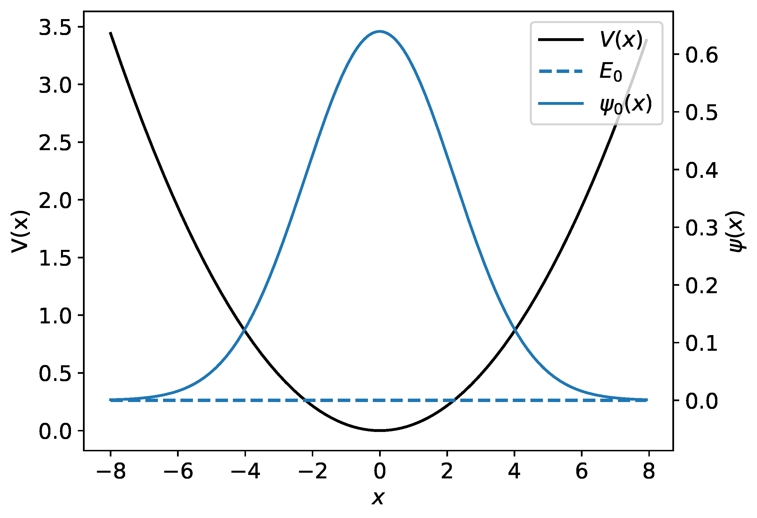
The harmonic potential together with the harmonic oscillator’s ground-state wave function and its associated energy are illustrated in Figure 1.
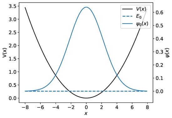
Figure 1.
The harmonic potential is shown by the black curve. The ground-state harmonic oscillator wave function and its associated energy are plotted in blue.
2.2. The Morse Potential
While small oscillations in a bound particle can often be approximated using the harmonic potential, in many situations, such as the interaction of two isolated atoms with each other (two-particle collisions or diatomic molecules, for example), the potential of interaction is better represented conceptually using the Morse potential [40,41,42]. It is described as
where D, a are the positive-value parameters of the potential, and is the position of the global minimum of the potential well. The Schrödinger equation for the potential is exactly solvable, giving the energies
where and
The wave functions for the energies are
where and and the associated Laguerre polynomials are defined by the formula
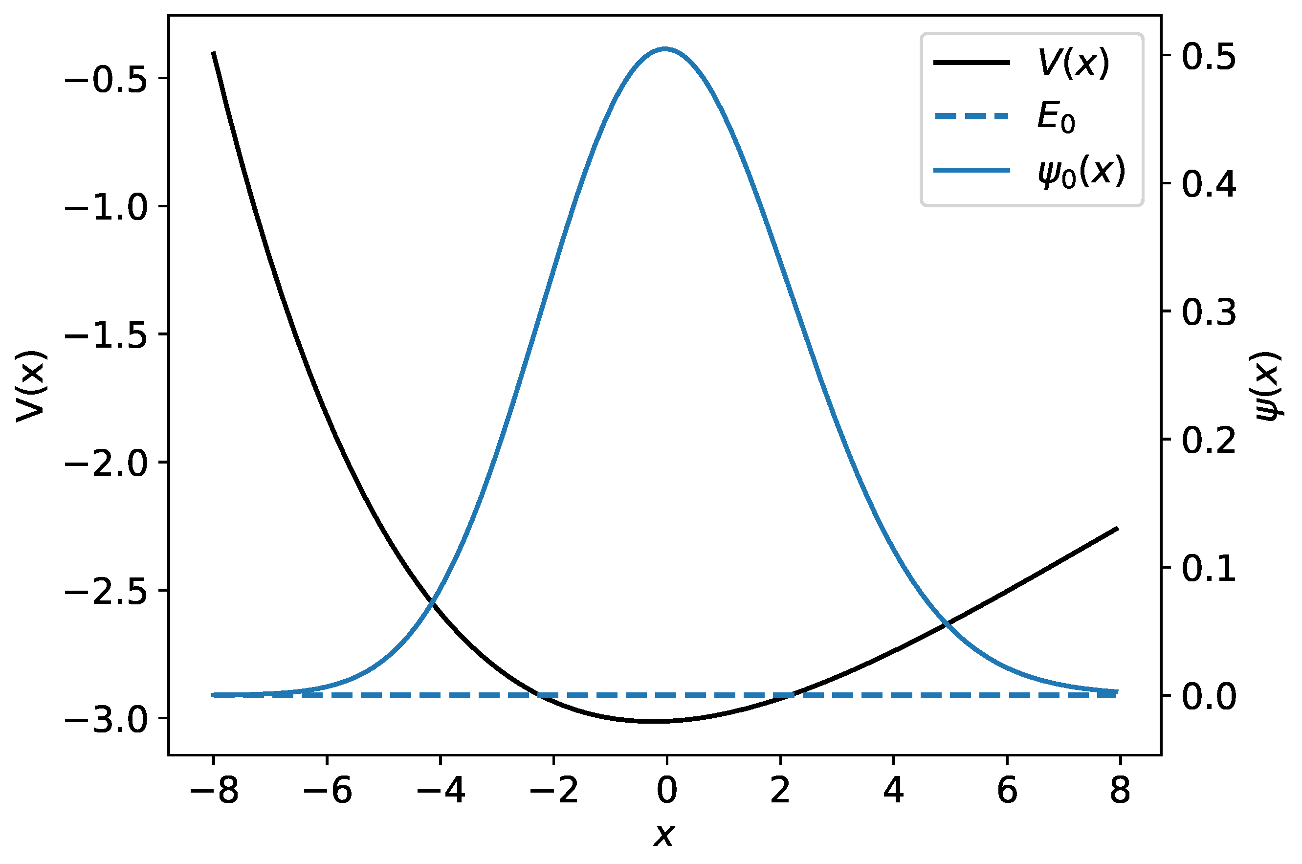
The Morse potential together with a wave function and its associated energy are illustrated in Figure 2.
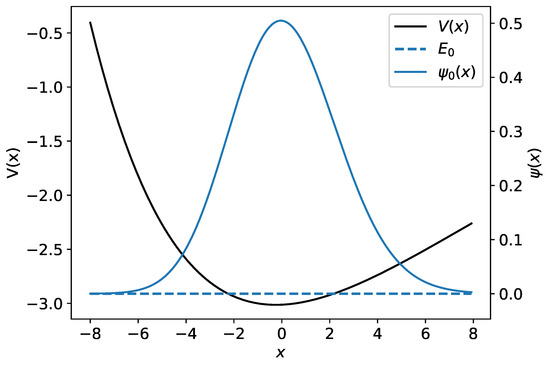
Figure 2.
The Morse potential is shown by the black curve. The ground-state wave function and its associated energy are plotted in blue.
2.3. Polynomial Potentials
Not all quantum mechanical systems admit analytic solutions. One can approximate various physical systems, with a potential well, using a polynomial potential of the form
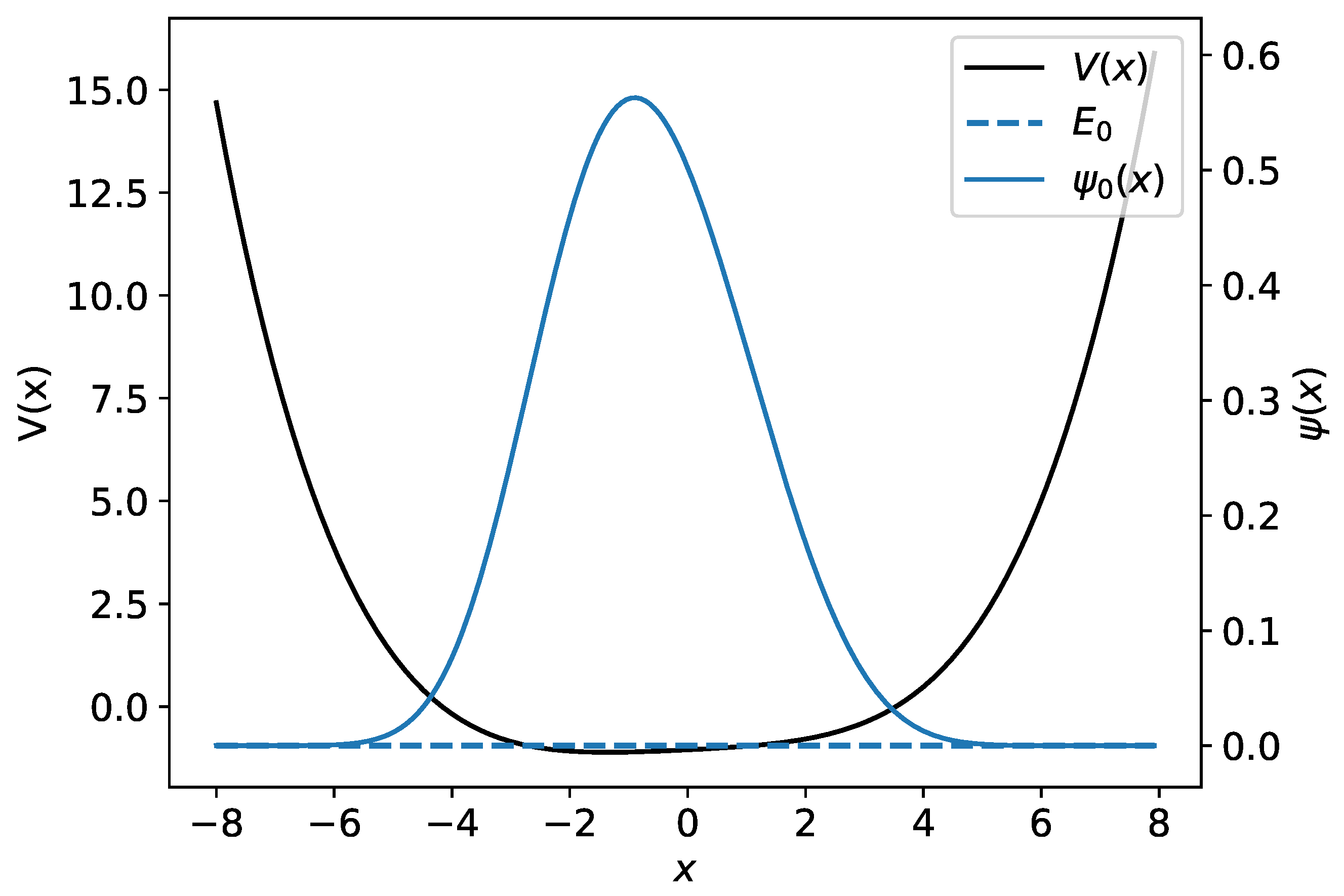
where are parameters with . Unfortunately, this system does not generally have an analytic solution, and therefore one has to use numerical methods to obtain the wave functions and the energy spectrum. Figure 3 gives an example of the polynomial potential of Equation (12) with and its ground-state wave function.
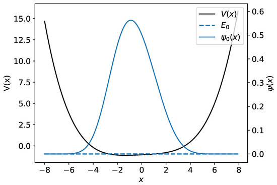
Figure 3.
An example of the polynomial potential is shown with a black line. The numerical wave function and its associated energy are plotted using the blue line.
2.4. Numerical Solutions to the Schrödinger Equation
Equation (1) can be solved numerically. Many different numerical methods exist [43], each with its own advantages and drawbacks. To solve differential equations like the Schrödinger equation, one can use propagation methods, e.g., Runge–Kuta [44,45] or Numerov’s [46], or variational methods, like finite-element methods, spectral methods, or pseudo-spectral methods. (Pseudo-)spectral methods have the advantage of allowing a Hamiltonian to be represented as a finite-dimensional matrix, reducing solving a differential equation into an eigenvalue problem. As such, they approximate the low-energy spectrum automatically and have good error properties compared to finite-elements methods.
We will use a particular pseudo-spectral method—the discrete-variable method—when we solve the Schrödinger equation numerically. In particular, this has the advantage that the coefficients of the eigenvectors of the Hamiltonian are simply wave functions in the position representation evaluated at grid points in space and therefore have an immediate and straightforward interpretation (see Equation (27)).
One of the numerical methods used for this purpose is recasting the Schrödinger equation as an eigenvalue problem. Let us suppose that a basis of square-integrable functions exists that spans the entire and is orthonormal and complete. Then, any solution can be decomposed into this basis
where the coefficients constitute a square-summable series, i.e., . Using the orthonormality of the basis, Schrödinger’s Equation (1) can be put into the form
where , . This is an infinite-dimensional eigenvalue problem for the eigenvector and the eigenvalue E.
Equation (14) is not treatable using numerical methods given its infinite dimension. However, one can replace this problem with an approximate problem
with a wave function
where determines where the infinite basis is truncated to a finite basis.
- The choice of the truncation dimension N is important for minimising the error, which comes from approximation. The coefficients vanish quickly enough such that after some term N, the error can be neglected. However, the choice of the correct truncation depends on the energy, and therefore the choice of N is important.
- The coefficients and have to be integrated. Numerical integration of the coefficients can be performed numerically or, in some cases, analytically.
The method called the discrete-variable method (DVR) [47,48,49,50,51,52,53] allows approximate values of the coefficients and to be obtained while minimising the errors. The coefficients of the kinetic energy operator are known analytically, while the potential energy operator has a diagonal form. The details of the method are provided in Appendix B. In particular, there are many different implementations [54,55,56], depending on the choice of the basis functions . Here, we will use the Fourier plane-wave basis [57], which is described below.
Let us consider a domain with a collection of N equally spaced points , where the length of the interval L and the spacing are related by . The collection of points forms a discrete grid which is used to calculate the coefficients of the Hamiltonian (note that the endpoint does not belong to this set). Moreover, let us assume that N is an even integer. The basis functions in which the wave functions are expanded are given by the sums of the plane waves in the form
where the wave numbers are given by
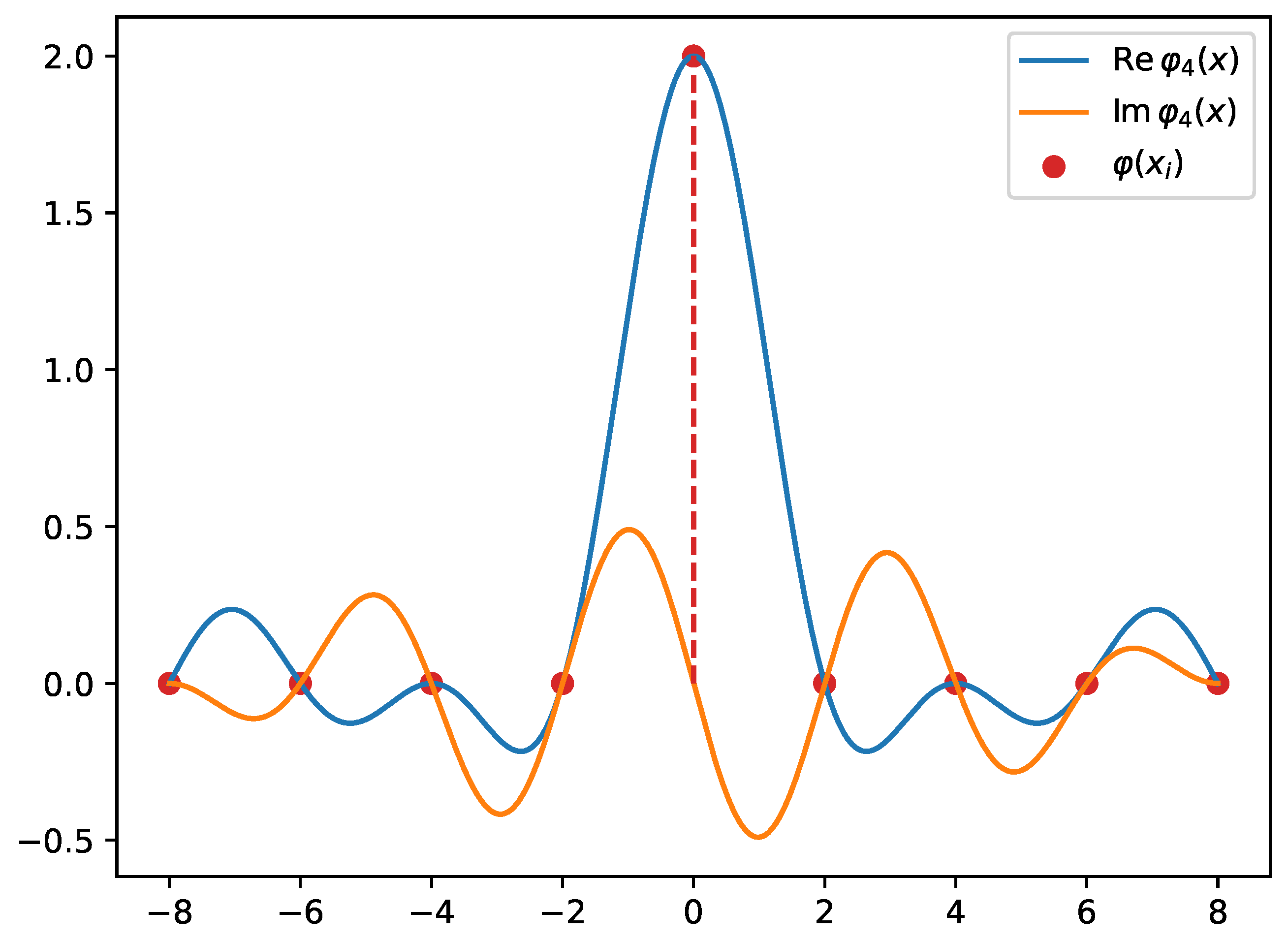
The basis functions , illustrated in Figure 4, on the grid are proportional to the Kronecker function
and are non-zero only at one of the grid points. The basis functions are linear combinations of plane waves. Plane waves are characterised by wave numbers. Because of the truncation, one can only represent a finite range of wave numbers. The lowest wave number that can be represented is
while the highest is
Because the wavelength and the wave number are related to each other
the constraints for the wave number imply that the minimal de Broglie wavelength that can be represented is
This also means that the kinetic energy is bounded
where m is the mass of the particle. This gives a clear bound on the energies of the states that can be described using DVR, and this is in agreement with our heuristic description of truncation of the basis, which we discussed above. In order to faithfully capture the states of higher energy, the number of grid points has to be augmented (or alternatively, the number of basis functions) N.
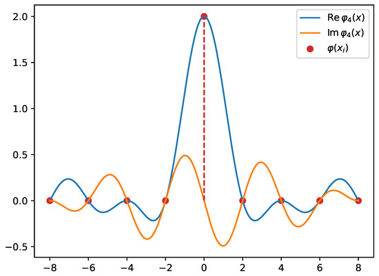
Figure 4.
The basis function defined on a domain with equidistant grid points. Notice that this basis function has 7 zeros, which correspond to other grid points (along with ) except . The dashed line points to the non-zero contribution of the basis function. This explains why the basis functions approximate the Dirac delta distribution on the grid.
The form of the kinetic energy operator coefficients on the plane-wave basis (which holds for N being an even integer) is as follows:
while the potential energy operator is diagonal, and its coefficients are obtained by just evaluating the potential on the grid
With the coefficients of the kinetic energy operator and the potential energy operator defined, one can solve Equation (15) as an eigenvalue problem. In particular, one can use the function scipy.linalg.eigh from the Python package scipy [58] to perform this operation on a computer.
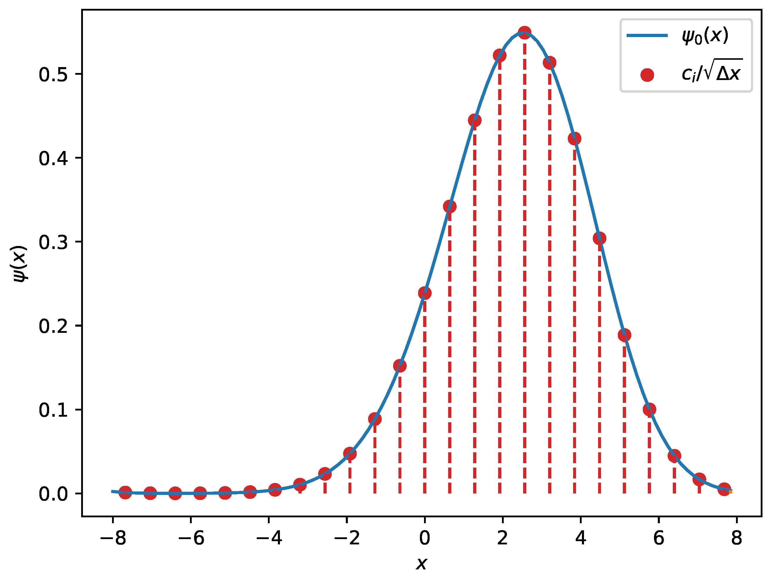
The coefficients of the wave function (16) are actually related to the values of the wave function on the grid points
Therefore, the wave function is an envelope along those coefficients, as illustrated in Figure 5. It is worthwhile noting that the discrete counterpart of the normalisation (2) implies
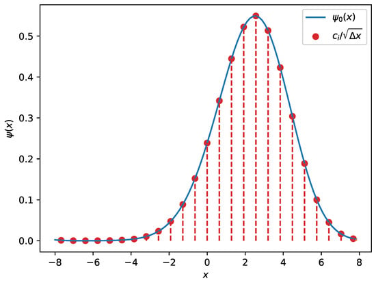
Figure 5.
An example of a wave function for a fifth-degree polynomial potential obtained using discrete-variable representation (DVR). The red dots illustrate the coefficients which are proportional to the wave function evaluated on the nodes. The red dashed lines represent the non-zero contributions from each basis function to the overall wave function.
3. Neural Network Models
In traditional computational sciences, one makes use of expert systems and dedicated algorithms (which come from statistics or the relevant sciences) in order to solve a given problem. These traditional methods have been augmented by the advent of machine learning techniques, where instead of encoding the dedicated algorithms directly, one lets the algorithm learn from the data, provided that a sufficient amount of relevant data exists. Often, that amount is extremely large.
Machine learning can respond to a variety of problems. Unsupervised learning concerns situations where only feature data is available, in the absence of target data, and the goal is to extract certain structures from the dataset itself. Common tasks in unsupervised learning are clustering (using clustering algorithms like k-means, hierarchical clustering, or DBSCAN) and dimensionality reduction (using, e.g., a principal component analysis, t-SNE, or autoencoders). Reinforcement learning is a paradigm of machine learning where a model is taught by offering rewards or punishments depending on the outcome, and it is used in the context of agent control, e.g., in robotics or game playing programmes. Meanwhile, unsupervised learning and reinforcement learning (and generative machine learning) are fields in their own right, and we are interested in supervised machine learning in particular. This is a subfield of machine learning which given pairs of (n-dimensional) input data and (m-dimensional) target data attempts to construct a function such that the difference between the actual target data and the prediction is minimised. The parameters describe the model, and their exact values are determined from the input and target data. Supervised learning is used mostly in prediction tasks, like classification and regression. It has been very successfully applied to the tasks of image recognition and classification, machine translation, machine transcription, and natural language processing and understanding, among many others.
One could ask how one would choose the function . The space of possible functions of this type is enormous, and the choice is between the possibility of encoding the relations behind the empirical data sufficiently and having as small a number of free parameters as possible. Various machine learning algorithms, like linear regression, logistic regression, and kernel support vector machines, provide different forms of functions f.
A particularly fruitful choice of architecture is a deep feedforward neural network or a multi-layer perceptron. For this particular choice of machine learning algorithm, the function is a composition of multiple simpler functions, which constitute layers
each one with its own, smaller set of parameters , . The fact that one can have multiple layers provided the name deep learning to neural networks.
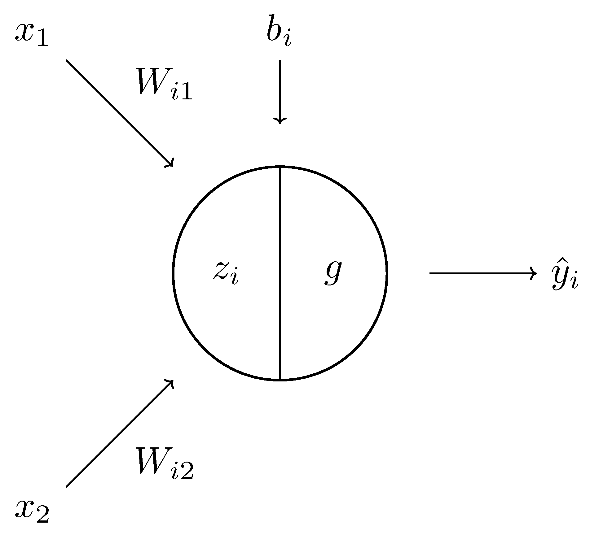
The basic building block of a feedforward neural network is a neuron [5,6], which is a function (c.f. Figure 6). Neurons can be grouped into collections to create fully connected layers, i.e., functions
where is the input, is the output, W is the mapping , are the parameters of the neural network, and g is a nonlinear function . One uses a nonlinear function g that is applied element-wise to allow the neural network to produce more complicated functions than just linear ones, which are too restrictive in terms of the possible outcomes. Popular choices for the nonlinear function g are the hyperbolic tangent tanh, the softmax function, and the rectified linear unit ReLU.

Figure 6.
A schematic diagram of a single neuron. It comprises a linear component and a nonlinear function g, which, composed, give the result .
Until now, we have described the architecture of the neural network depending on its weights , which can give us the target values as a function of the input values. However, starting from a random choice of weights would lead to a model that would not correctly predict the data, as the space of parameters would be very large. Therefore, there are two issues to resolve:
- How can one evaluate the correctness of the predictions of a neural network?
- Given the correctness, how one can improve the weights iteratively so that they give better results?
The first question is answered using the so-called loss function. Loss functions are non-negative definite scalar functions
which depend on the target data y and the prediction . They are chosen in such a way that they obtain the minimum when the prediction is equal to the target data , and any difference contributes positively. Loss functions have a probabilistic interpretation in terms of maximising the log-likelihood; however, usually, it is sufficient to choose the one that is most suitable for a given problem. In the context of classification problems, one tends to use the logarithm of sigmoid or softmax functions, while in the context of regression problems, the mean squared error is used:
Having resolved the first issue, we can now focus on a way to iteratively improve the model’s weights so that it minimises the loss function. The method used for this purpose is called gradient descent [59]. One can imagine the multi-dimensional surface given by the loss function as a function of the weights of the neural network
This surface will possibly have multiple minima—a global minimum and a collection of local minima. Ideally, one desires an algorithm which provides the location of the global minimum and therefore the best possible weights given the input and target data. However, this is not feasible, and a local method is used where the weights along the direction of the gradient of the loss function are updated:
where is called the learning rate. The simplest choice for the learning rate is a constant number. However, in deep learning, various adaptive algorithms have been developed that adjust the learning rate dynamically as a function of the gradients, like AdaGrad [60], RMSprop, and Adam [61].
In order to effectively perform gradient descent, one needs to quickly compute the gradients of the loss function. This is conducted with the help of an efficient back-propagation technique which computes the gradients using the chain rule by keeping track of the graph of elementary mathematical operations (e.g., addition, multiplication, exponentiation, etc.) that build up the loss function.
Given that the input and target data contains multiple (multi-dimensional) points, one can make a choice on when to update the weights. If the update happens after adding up the gradients for all of the points, then the gradient descent is deterministic. However, by bundling the data points into batches, computing the gradient for each batch, and updating the weights, one can stochastically approximate the deterministic gradient. This method is known under the name of stochastic gradient descent. Especially for high-dimensional problems, stochastic gradient descent reduces the computational complexity and therefore the demand on the computer hardware, at the price of a lower convergence rate.
4. Machine Learning Training and Prediction
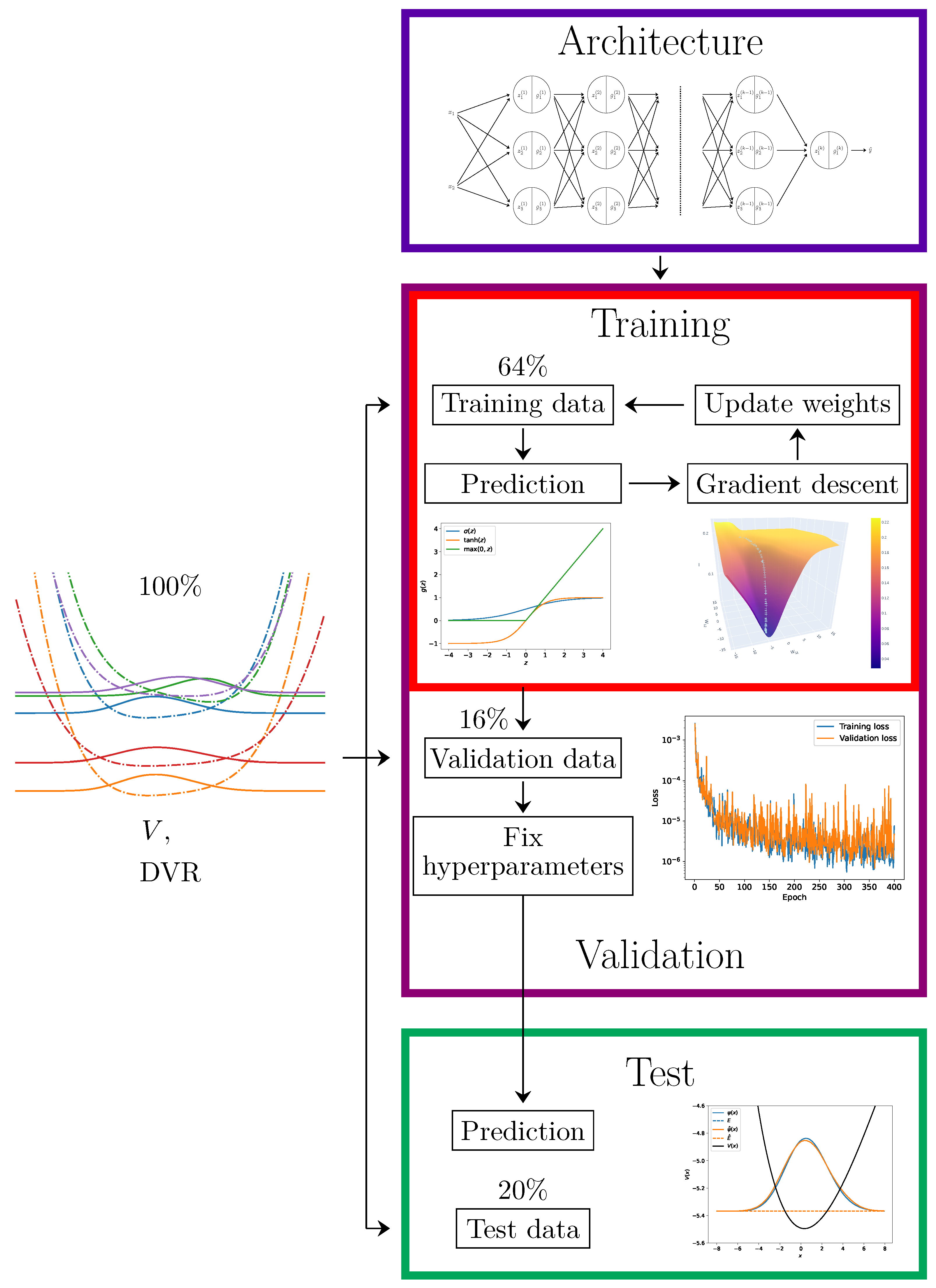
The process that uses stochastic gradient descent in order to find the model weights that best represent the data is known under the name of training of the machine learning model (which we illustrate schematically in Figure 7). If one trains a model on the whole set of pairs of input data and target data, one can expect (under certain assumptions) that the loss function will either monotonically tend towards a local minimum or start to oscillate around it. Therefore, if the loss function on the data which are used for the training is the only measure of quality of the model, then spending more and more time on training iterations would give a better model. In reality, however, this is not the case—and this is related to the concept of the generalisability of the model.
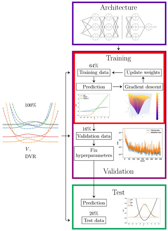
Figure 7.
A schematic of the process of training a neural network. The initial dataset is split into 3 parts: the training data, the validation data, and the test data. The neural network model starts with a chosen architecture with randomly drawn parameters (blue rectangle). For a given number of epochs, the models are trained on training data using gradient descent (red rectangle)—within the insets, popular activation functions and the evolution of the parameters during gradient descent are depicted. After this, if there are models with differing parameters, they will be compared on the validation data, and the most performant is chosen (violet rectangle)—in the inset, the loss function as a function of a hyperparameter (i.e., an epoch) is plotted. Finally, the model’s predictions are tested against the test data (green rectangle)—in the inset, the target data and the data predicted by the model are plotted.
Let us imagine that the initial data used for training comes from some larger probabilistic distribution and as such constitutes just a sample taken from this distribution. If the sample does not faithfully reproduce all of the properties of the probabilistic distribution but rather exhibits some random aberrations (e.g., the initial data consists of more points at a distance from the mean than expected, or it is skewed to one side of the mean), then the machine learning model will also learn the aberrations from the sample dataset. Once one evaluates the model on other data generated from the initial probability distribution, the model will not perform well because it learned the random properties of the training data, which were only present in the sample. This phenomenon is known under the name of overfitting—as opposed to underfitting, which happens when the model is not trained for long enough and does not learn the properties of the training data sufficiently.
Therefore, in order to prevent overfitting, one puts aside part of the initial data and avoids training the machine learning model on it. This part of the dataset that is put aside is called the test data. If the loss function evaluated on the training data is approximately equal to the loss on the test data after the process of training, one knows that both overfitting and underfitting have been prevented.
The situation is more complicated when one wants to test the performance of multiple different models or a model that has various adjustable hyperparameters (like the number of layers of the neural network, the training time, etc.). In that case, using the results of evaluating the models on the test data to choose the hyperparameters would not indicate under-/overfitting correctly. To aid with this, a validation procedure is developed. One proceeds with dividing the initial data into three distinct parts which have different purposes:
- Training data—the largest part of the initial data, which is used to train the machine learning models;
- Validation data—the part of the initial data which is used to determine the hyperparameters of the model;
- Test data—the part of the initial data (∼20%) which is used to determine the quality of the model and check whether it is under- or overfitted.
This does leave a particular issue, however—if the initial data is limited (e.g., it is observational data related to markets, climate, weather, etc.) and cannot be generated easily (as is the case in our application to quantum mechanics in Section 5), then setting aside both the training and validation data significantly cuts into the amount of data points that can be used to train the machine learning model. The technique of cross-validation has been developed to avoid this problem.
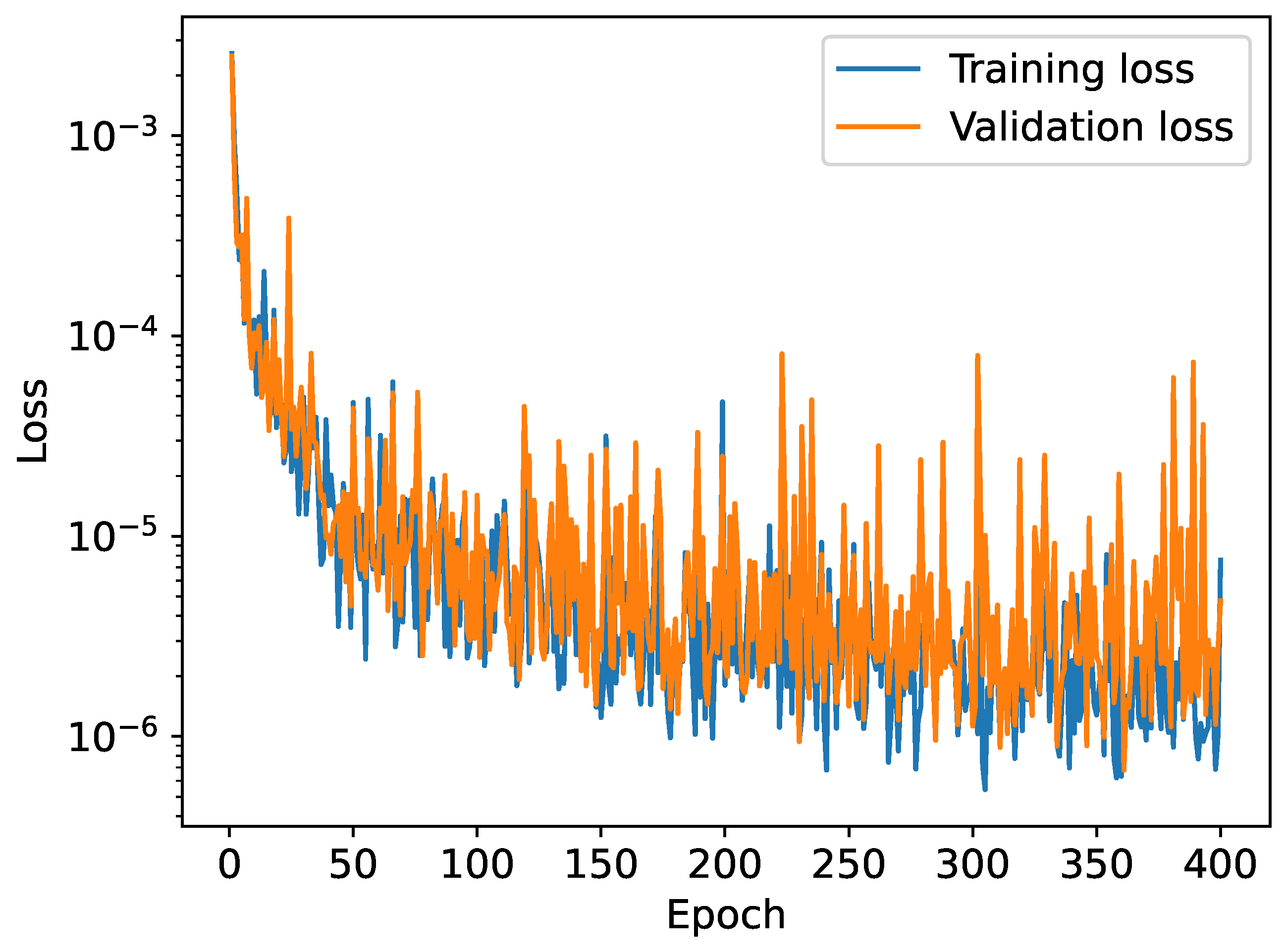
In the case of neural networks, outside of the quantities which determine the architecture (like the number of layers or the amount of neurons), the number of epochs is the most obvious hyperparameter. Training a neural network on the entirety of the training data once over using stochastic gradient descent constitutes one epoch. Since the training can be repeated indefinitely, reducing (under certain conditions) the training loss each time, the number of epochs equivalently measures the time spent training the model. One can set an early stopping condition on the training process that is applied when the validation loss ceases to improve. Figure 8 illustrates this procedure.
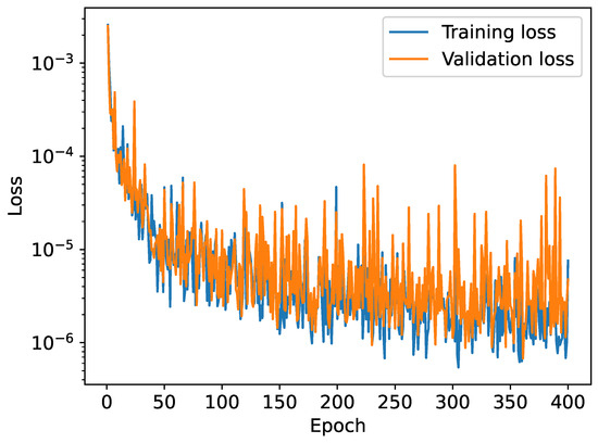
Figure 8.
Training and validation loss as a function of the epoch when trained on a dataset of 5000 potentials.
5. Neural Networks for Solving the Schrödinger Equation
In order to illustrate the above concepts, we developed a Python -based Jupyter notebook in which a fully connected neural network was trained to predict the wave functions of a quantum mechanical system given its defining potential.
The initial data constitutes the pairs , of potentials and wave functions evaluated on N equidistant grid points. These wave functions are the solutions to the Schrödinger equation with the potentials V obtained using the plane-wave DVR method, implemented using numpy [62] version 1.24.3 and scipy version 1.10.1 Python packages. We have chosen to take as the default value.
The training data and the validation data is composed of polynomial potentials, with the coefficients of the polynomials randomly chosen from uniform distributions, which ensures that the neural network can learn a variety of different potentials. The degree of the polynomial potential as well as the shape of the uniform probability distributions can be adjusted.
In addition to the training and validation data, we also use the test data to evaluate the performance of the final model. The test data contains polynomial potentials drawn from the same distribution as the training and validation data. Moreover, we also use (separately) data points generated from the harmonic oscillator and Morse potentials. Since these potentials admit analytical solutions, we use the analytical solutions instead of the numerical solutions provided by the DVR method. While the harmonic oscillator potential is a subtype of polynomial potential, the Morse potential is not (as it involves an exponential function) and cannot belong to the training data. These polynomials are added to the test data because it is instructive to learn how our neural network generalises to different, previously unseen potentials.
The Python package sklearn [63] version 1.3.0 is used to split the initial data containing (by default) 5000 polynomial potentials and wave functions between the training data and the validation data.
The machine learning model is supposed to take a potential evaluated on N points as an input and give a wave function evaluated on the same points as an output
The fully connected neural network that we use is composed of five layers—four of them are hidden layers, and the last one is the output layer. The hidden layers are composed using ReLU functions and have the output sizes 256, 256, 128, and 128, while the output layer does not have a nonlinear component, and its output size is equal to the number of grid points N, which is also the size of the input of the first layer. Each layer is separated by a dropout layer, which is used only during training—dropout selectively sets the output of individual neurons randomly to zero, which has been shown to improve the training by introducing noise into the process. At the level of implementation, the neural network uses the tensorflow version 2.12.1 [64] Python package, in particular its high-level keras interface.
The loss function which is used to evaluate the performance of the model is the mean squared error between the initial wave functions obtained either analytically or numerically through DVR and the predicted wave functions , which are the output of the neural network
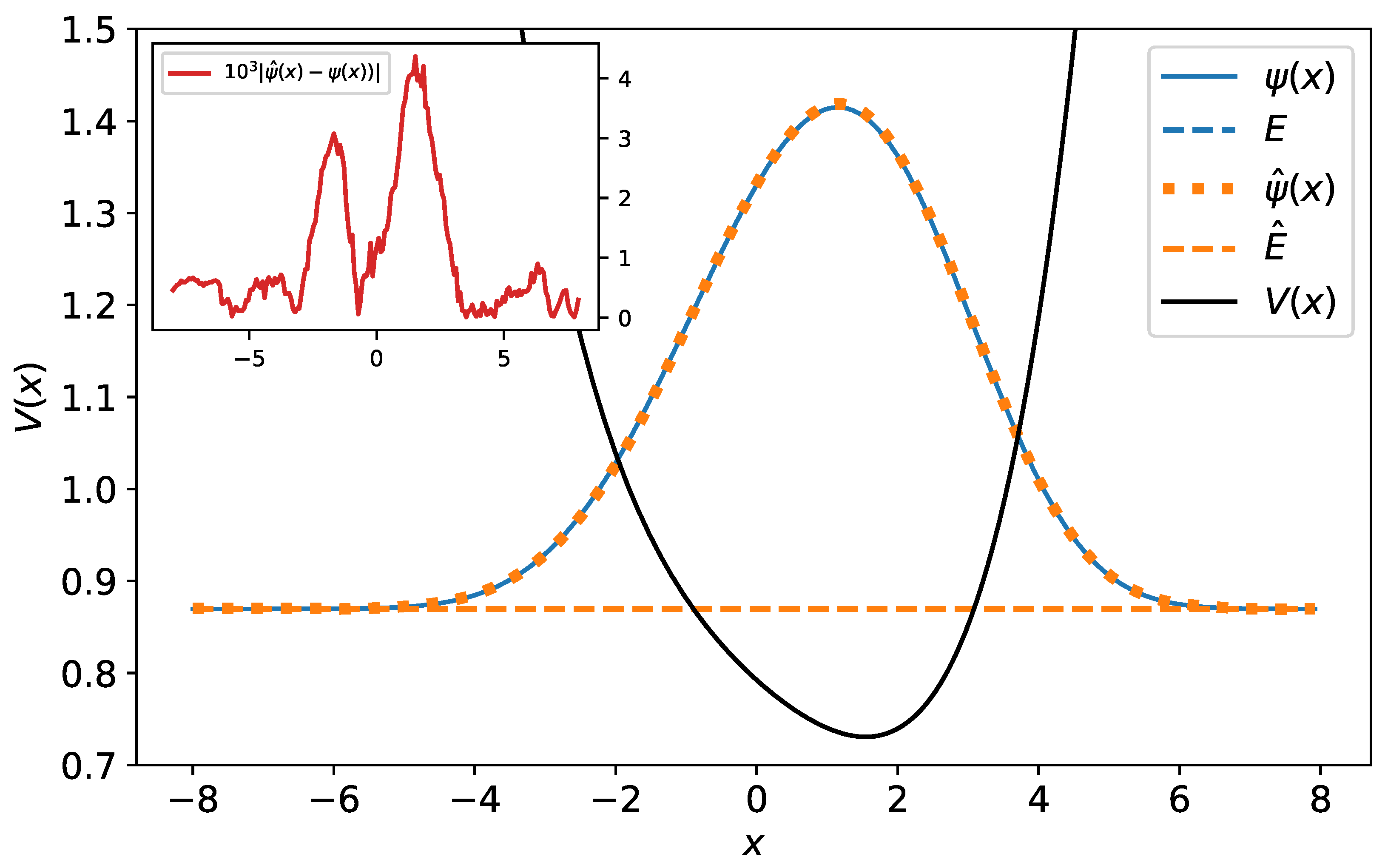
One trains the neural network with an early stopping condition which relies on the validation loss not improving for a given amount of epochs (by default 20), as well as with the initial learning rate of adjusted by the Adam algorithm. We summarise all of this information in Table 1. Afterwards, the loss of the data with polynomial potentials can be examined, as can the graphs of the original and predicted wave functions be inspected visually (c.f. Figure 9). The wave functions are really close, as one would expect. We also examine the energies of the original and predicted wave functions, using the discrete analogue of Equation (3):

Table 1.
Table summarising the datasets, neural network architecture, loss function, and training process used.
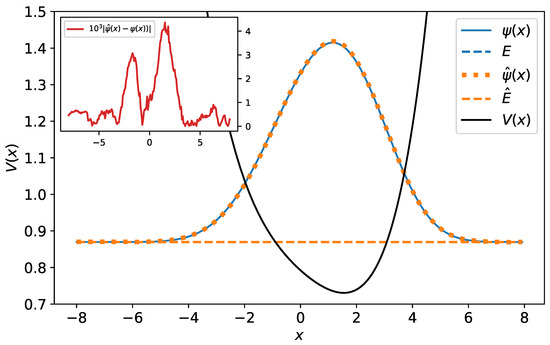
Figure 9.
The original and predicted wave functions for polynomial potential. The wave functions are drawn with their energies as a reference level. As one sees, the original and predicted wave functions are almost identical—their relative error equals . The energy reference line of the original wave function (blue dashed line) is completely covered by the energy reference line of the predicted wave function (orange dashed line). In the inset, the difference between the original and predicted wave function has been plotted.
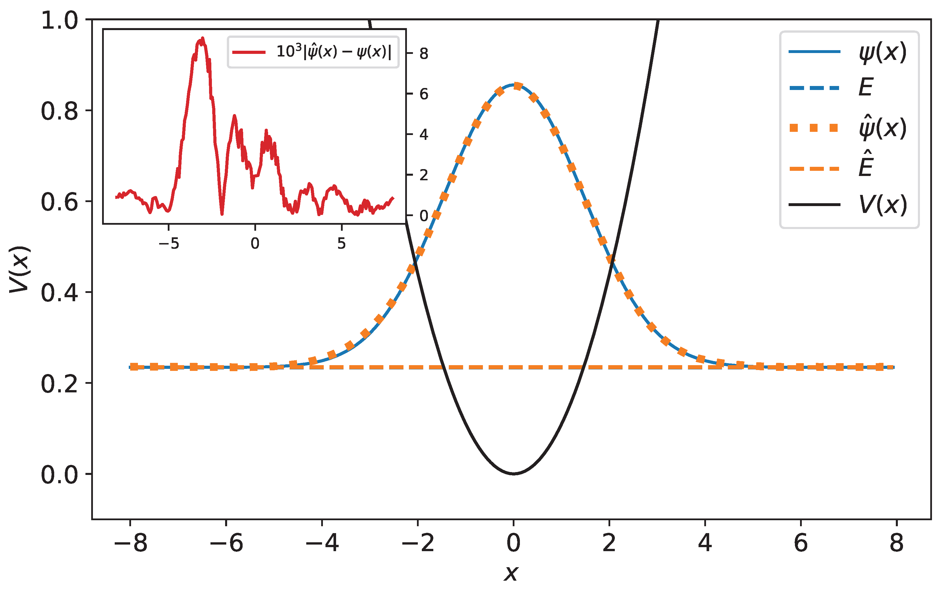
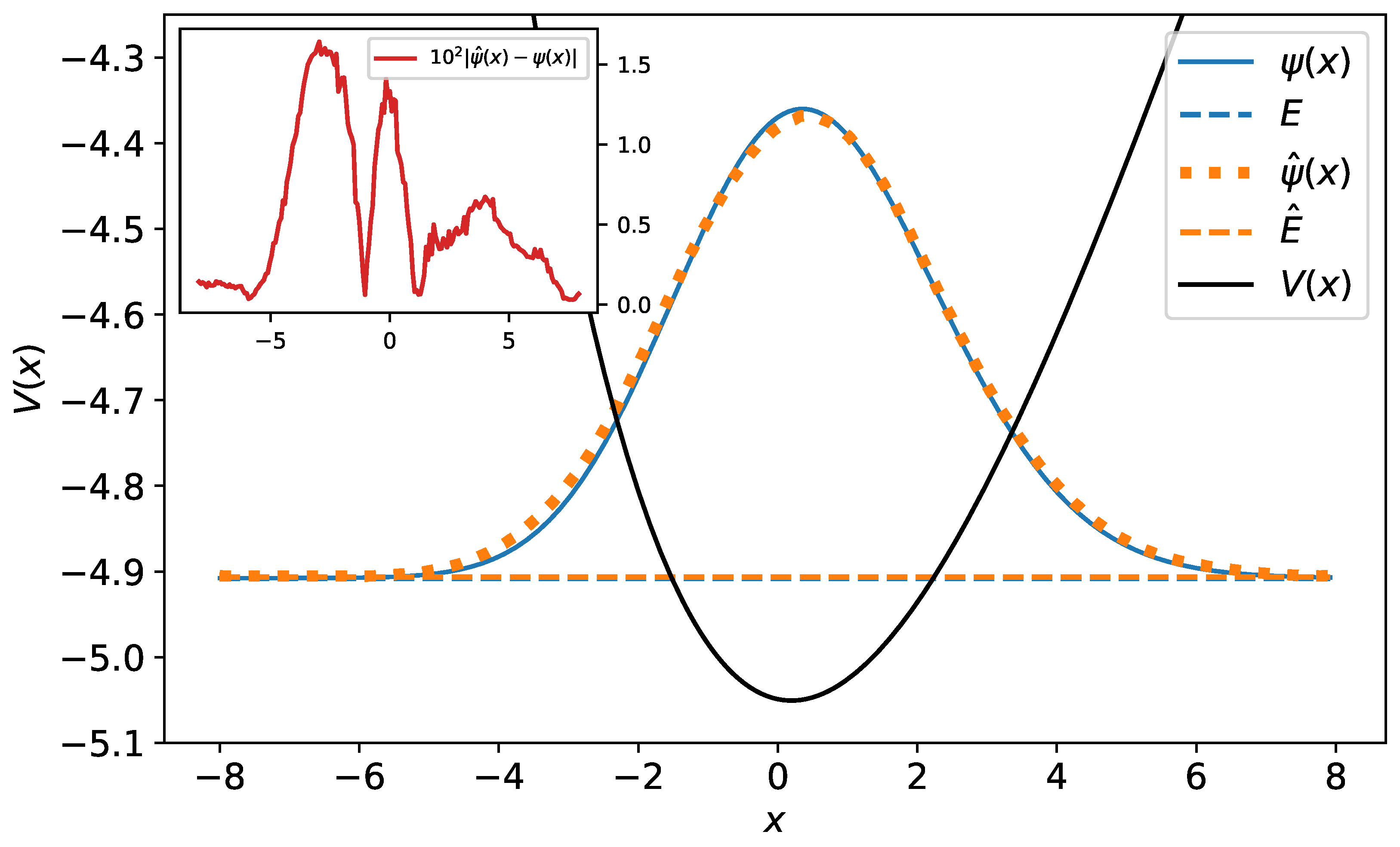
In addition to the polynomial potentials, we also examine the performance of the neural network on harmonic and Morse potentials. As expected, the model performs worse on the Morse potential compared to polynomial potentials—the losses are approximately an order of magnitude higher. This is also evident from the wave functions; examples are shown in Figure 10 and Figure 11. This is because the Morse potential (7) is described by an analytic function and therefore admits an expansion in terms of an infinite series. Because the neural network was trained only on polynomials of the fifth degree, it does not generalise sufficiently well. One can improve the score for the Morse potential by using higher-order polynomials in the training data—however, it is surprising that the neural network is capable of relatively close predictions even when trained on fifth-degree polynomials. Overall, we conclude that the machine learning model trained on relatively low-degree polynomials can capture the wave functions of the Morse potential (which are given by exponential functions). We summarise these results in Table 2.
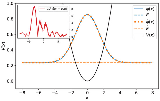
Figure 10.
Original and predicted wave functions for harmonic oscillator. The wave functions are drawn with their energies as a reference level. The original and predicted wave functions are very close—their relative error equals 0.32%. In the inset, the difference between the original and predicted wave function has been plotted.
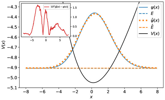
Figure 11.
The original and predicted wave functions for the Morse potential. The wave functions are drawn with their energies as a reference level. Their relative error equals . In the inset, the difference between the original and predicted wave functions has been plotted.
6. Conclusions
In this paper, we described a Python-based Jupyter notebook developed with the purpose of pedagogically introducing concepts from both quantum mechanics and machine learning. We introduced various types of Schrödinger equations (depending on the potentials) and an efficient way to numerically obtain solutions to them using the DVR method. This constituted the initial dataset which we used to train a fully connected neural network, which predicted the wave function given a potential as an input. The developed Jupyter notebook is employed during the classes within the Erasmus Mundus Quarmen Master programme. During the programme, students learn the basics of machine learning by first implementing a single-layer perceptron and then multi-layer ones in Python. Afterwards, they are acquainted with the keras interface from the tensorflow package. Students also learn how to implement numerical solvers which can be used to study the quantum problems described by the Schrödinger equation. The notebook presented with this paper is used to combine the ideas which were previously learned by the participants from the programme. We hope that this type of introduction will be beneficial to students, who can later tackle fully fledged and realistic problems involving applying machine learning to quantum physics and quantum chemistry.
Author Contributions
Conceptualization, V.K. and M.A.A.; Methodology, F.G., D.C. and M.A.A.; Software, M.K.P., F.G. and D.C.; Formal analysis, F.G., D.C., V.K. and M.A.A.; Investigation, M.K.P., F.G. and D.C.; Writing—original draft, M.K.P.; Writing—review & editing, M.K.P., V.K. and M.A.A.; Visualization, M.K.P.; Supervision, V.K. and M.A.A.; Project administration, M.A.A.; Funding acquisition, M.A.A. All authors have read and agreed to the published version of the manuscript.
Funding
This research was funded by the U.S. National Science Foundation grant number PHY-2409570. This work also benefited from French state aid under France 2030 (QuanTEdu-France), bearing the reference ANR-22-CMAS-0001. Funding has also been recieved from the Transatlantic Mobility Program of the Office for Science and Technology of the Embassy of France in the United States, Programme National “Physique et Chimie du Milieu Interstellaire” (PCMI) of CNRS/INSU; the programme “Accueil des chercheurs étrangers” of CentraleSupélec. M.A. and V.K. acknowledge the co-funding from the EU project DigiQ: Digitally Enhanced European Quantum Technology Master.
Data Availability Statement
The original contributions presented in this study are included in the article. Further inquiries can be directed to the corresponding author.
Acknowledgments
The stimulating discussions with Marino Marsi in building the course are gratefully acknowledged.
Conflicts of Interest
The authors declare no conflicts of interest.
Appendix A. Integration by Quadrature
The integrals can be approximated by sums. One of the simplest ways to approximate integrals is a Riemann sum
where , , with and . For the Riemann integrable functions , we know that the Riemann sum will converge to the integral when —however, how fast that convergence will be is not guaranteed.
A more sophisticated version of evaluating integrals uses quadrature [65]. For a certain class of functions, the integral is equal to a sum
where is the interval of integration on the which functions are defined, is a positive weight function, are suitably chosen nodes, and are suitably chosen weights. The function f which one integrates expands into
where are expansion coefficients and are orthogonal polynomials (e.g., Legendre polynomials, Laguerre polynomials, or Hermite polynomials). The sum (A2) is exact if is a polynomial of a degree at most (i.e., )—otherwise, it provides us only with an approximation of the integral—the reader should think of the equality sign being replaced with ≈ in that case.
The nodes are chosen so that they constitute the roots of the polynomial. The orthogonality condition which is satisfied by the polynomials also determines the weight function
Finally, the weights can be determined analytically.
Appendix B. DVR
Appendix B.1. Plane-Wave DVR
Equipped with a way to integrate using a Riemann sum or a quadrature, let us consider the expansion of wave functions into plane waves
where are expansion coefficients, N is the truncation dimension, and the wave number for . The basis functions are just the plane waves
with the wave numbers given above. The plane waves are orthonormal
One could try to approximate this using the Riemann sum (A1) with equidistant grid points defined below that equation. However, the plane waves do in fact satisfy a discrete orthogonality condition like this exactly
which can be shown by summing a geometric series. Then, the expansion coefficients in Equation (A5) are given by the finite sum
Substituting this back into Equation (A5), one can arrive at
which then can be used to provide an alternative basis decomposition
where the coefficients are given by
while the new basis functions
The transformation from the basis to the basis is unitary. Usually, one sets so that those two bases are of the same dimension—we will make that assumption from now on.
The basis elements can be re-summed so that they take the form
in the first case using the sum of a geometric series. It is clear that this basis function constitutes a Kronecker delta on the grid points
in agreement with what Figure 4 demonstrates.
Using the Riemann sum approximation and the basis elements above, one can estimate the kinetic energy operator matrix elements, as well as the potential energy operator matrix elements. The potential operator is in fact diagonal:
where one uses Equation (A15) to remove the sum. The kinetic energy operator has the form
This can be computed using the values of the derivatives of the basis elements evaluated on points
or on the point
In the same way, one can derive the coefficients of the momentum operator ()
Appendix B.2. Orthogonal Polynomial DVR
Instead of relying on the Riemann sum approximation, one can proceed with the more sophisticated process of integration by quadrature (A2). To this end, one can choose an expansion of the wave function into a basis of the type
where are the expansion coefficients, is the truncation dimension, and are basis functions in the form of orthogonal polynomials. Using the orthogonality of the basis functions (A4), one can compute the coefficients
where the second equality is exact (and not an approximation) if . By inserting this expression back into the wave function decomposition and re-arranging the terms, one can write another decomposition
The coefficients of this decomposition are given by
while the new basis elements
The transformation from the basis of orthogonal polynomials to the basis of functions can be shown to be unitary; i.e., it is physically equivalent.
The coefficients of the kinetic energy operator and the potential energy operator can be obtained on this basis. The potential operator is in fact diagonal:
where the second equality is exact when and an approximation otherwise. The kinetic energy can be calculated using
where the second equality is exact if and an approximation otherwise. The explicit expression depends on the choice of the orthogonal polynomial [54,55], which can be, e.g., a Laguerre polynomial, a Legendre polynomial, a Hermite polynomial, etc.
The two bases will have the same dimension when .
References
- Boser, B.E.; Guyon, I.M.; Vapnik, V.N. A training algorithm for optimal margin classifiers. In Proceedings of the Fifth Annual Workshop on Computational Learning Theory, New York, NY, USA, 27–29 July 1992; COLT ’92. pp. 144–152. [Google Scholar] [CrossRef]
- Cortes, C.; Vapnik, V. Support-vector networks. Mach. Learn. 1995, 20, 273–297. [Google Scholar] [CrossRef]
- Burges, C.J.; Schölkopf, B.; Smola, A.J. Advances in Kernel Methods: Support Vector Learning; The MIT Press: Cambridge, MA, USA, 1998. [Google Scholar] [CrossRef]
- Goodfellow, I.; Bengio, Y.; Courville, A.; Bengio, Y. Deep Learning; MIT Press: Cambridge, UK, 2016; Volume 1. [Google Scholar]
- Gatti, F. Artificial Neural Networks. In Machine Learning in Geomechanics 1; John Wiley & Sons, Ltd.: Hoboken, NJ, USA, 2024; Chapter 5; pp. 145–236. [Google Scholar] [CrossRef]
- Gatti, F. Artificial Neural Networks. In Machine Learning in Geomechanics 2; John Wiley & Sons, Ltd.: Hoboken, NJ, USA, 2024; Chapter 5; pp. 185–275. [Google Scholar] [CrossRef]
- McCulloch, W.S.; Pitts, W. A logical calculus of the ideas immanent in nervous activity. Bull. Math. Biophys. 1943, 5, 115–133. [Google Scholar] [CrossRef]
- ROSENBLATT, M. Some Purely Deterministic Processes. J. Math. Mech. 1957, 6, 801–810. [Google Scholar]
- Rosenblatt, F. The perceptron: A probabilistic model for information storage and organization in the brain. Psychol. Rev. 1958, 65, 386–408. [Google Scholar] [CrossRef] [PubMed]
- Rosenblatt, F. Principles of Neurodynamics; Spartan: New York, NY, USA, 1962. [Google Scholar]
- Hecht-Nielsen, R. Kolmogorov’s Mapping Neural Network Existence Theorem. In Proceedings of the IEEE First International Conference on Neural Networks (San Diego, CA); IEEE: Piscataway, NJ, USA, 1987; Volume III, pp. 11–13. [Google Scholar]
- Hecht-Nielsen, R. III.3—Theory of the Backpropagation Neural Network. In Neural Networks for Perception; Wechsler, H., Ed.; Academic Press: Cambridge, MA, USA, 1992; pp. 65–93. [Google Scholar] [CrossRef]
- Cybenko, G. Approximation by superpositions of a sigmoidal function. Math. Control. Signals Syst. 1989, 2, 303–314. [Google Scholar] [CrossRef]
- Leshno, M.; Lin, V.Y.; Pinkus, A.; Schocken, S. Multilayer feedforward networks with a nonpolynomial activation function can approximate any function. Neural Netw. 1993, 6, 861–867. [Google Scholar] [CrossRef]
- Rumelhart, D.E.; Hinton, G.E.; Williams, R.J. Learning representations by back-propagating errors. Nature 1986, 323, 533–536. [Google Scholar] [CrossRef]
- Rumelhart, D.E.; Hinton, G.E.; Williams, R.J. Learning internal representations by error propagation. In Parallel Distributed Processing; Rumelhart, D.E., McClelland, J.L., Eds.; MIT Press: Cambridge, UK, 1986; Volume 1, Chapter 8; pp. 318–362. [Google Scholar]
- Hinton, G.E.; Osindero, S.; Teh, Y.W. A Fast Learning Algorithm for Deep Belief Nets. Neural Comput. 2006, 18, 1527–1554. [Google Scholar] [CrossRef]
- Schölkopf, B.; Platt, J.; Hofmann, T. Greedy Layer-Wise Training of Deep Networks. In Advances in Neural Information Processing Systems 19: Proceedings of the 2006 Conference; The MIT Press: Cambridge, MA, USA, 2007; pp. 153–160. [Google Scholar]
- Lecun, Y.; Bottou, L.; Bengio, Y.; Haffner, P. Gradient-based learning applied to document recognition. Proc. IEEE 1998, 86, 2278–2324. [Google Scholar] [CrossRef]
- Hochreiter, S.; Schmidhuber, J. Long Short-Term Memory. Neural Comput. 1997, 9, 1735–1780. [Google Scholar] [CrossRef]
- Vaswani, A.; Shazeer, N.; Parmar, N.; Uszkoreit, J.; Jones, L.; Gomez, A.N.; Kaiser, L.; Polosukhin, I. Attention is all you need. In Proceedings of the 31st International Conference on Neural Information Processing Systems, Red Hook, NY, USA, 4–9 December 2017; NIPS’17. pp. 6000–6010. [Google Scholar]
- Carleo, G.; Cirac, I.; Cranmer, K.; Daudet, L.; Schuld, M.; Tishby, N.; Vogt-Maranto, L.; Zdeborová, L. Machine learning and the physical sciences. Rev. Mod. Phys. 2019, 91, 045002. [Google Scholar] [CrossRef]
- Dawid, A.; Arnold, J.; Requena, B.; Gresch, A.; Płodzień, M.; Donatella, K.; Nicoli, K.A.; Stornati, P.; Koch, R.; Büttner, M.; et al. Modern applications of machine learning in quantum sciences. arXiv 2022, arXiv:quant-ph/2204.04198. [Google Scholar]
- Carrasquilla, J. Machine learning for quantum matter. Adv. Physics X 2020, 5, 1797528. [Google Scholar] [CrossRef]
- Julian, D.; Koots, R.; Pérez-Ríos, J. Machine-learning models for atom-diatom reactions across isotopologues. Phys. Rev. A 2024, 110, 032811. [Google Scholar] [CrossRef]
- Guan, X.; Heindel, J.P.; Ko, T.; Yang, C.; Head-Gordon, T. Using machine learning to go beyond potential energy surface benchmarking for chemical reactivity. Nat. Comput. Sci. 2023, 3, 965–974. [Google Scholar] [CrossRef] [PubMed]
- Krenn, M.; Landgraf, J.; Foesel, T.; Marquardt, F. Artificial intelligence and machine learning for quantum technologies. Phys. Rev. A 2023, 107, 010101. [Google Scholar] [CrossRef]
- Carleo, G.; Troyer, M. Solving the quantum many-body problem with artificial neural networks. Science 2017, 355, 602–606. [Google Scholar] [CrossRef]
- Yıldız, c.; Heinonen, M.; Lahdesmäki, H. ODE2VAE: Deep generative second order ODEs with Bayesian neural networks. In Proceedings of the 33rd International Conference on Neural Information Processing Systems; Curran Associates Inc.: Red Hook, NY, USA, 2019. [Google Scholar]
- Huang, S.; Feng, W.; Tang, C.; He, Z.; Yu, C.; Lv, J. Partial Differential Equations Meet Deep Neural Networks: A Survey. In IEEE Transactions on Neural Networks and Learning Systems; IEEE: New York, NY, USA, 2025; pp. 1–21. [Google Scholar] [CrossRef]
- E, W.; Yu, B. The Deep Ritz Method: A Deep Learning-Based Numerical Algorithm for Solving Variational Problems. Commun. Math. Stat. 2018, 6, 1–12. [Google Scholar] [CrossRef]
- Hermann, J.; Schätzle, Z.; Noé, F. Deep-neural-network solution of the electronic Schrödinger equation. Nat. Chem. 2020, 12, 891–897. [Google Scholar] [CrossRef]
- Zhang, Y.; Jiang, B.; Guo, H. SchrödingerNet: A Universal Neural Network Solver for the Schrödinger Equation. J. Chem. Theory Comput. 2025, 21, 670–677. [Google Scholar] [CrossRef] [PubMed]
- Nakajima, M.; Tanaka, K.; Hashimoto, T. Neural Schrödinger Equation: Physical Law as Deep Neural Network. IEEE Trans. Neural Networks Learn. Syst. 2022, 33, 2686–2700. [Google Scholar] [CrossRef] [PubMed]
- Raissi, M.; Perdikaris, P.; Karniadakis, G. Physics-informed neural networks: A deep learning framework for solving forward and inverse problems involving nonlinear partial differential equations. J. Comput. Phys. 2019, 378, 686–707. [Google Scholar] [CrossRef]
- Han, J.; Zhang, L.; E, W. Solving many-electron Schrödinger equation using deep neural networks. J. Comput. Phys. 2019, 399, 108929. [Google Scholar] [CrossRef]
- Kluyver, T.; Ragan-Kelley, B.; Pérez, F.; Granger, B.; Bussonnier, M.; Frederic, J.; Kelley, K.; Hamrick, J.; Grout, J.; Corlay, S.; et al. Jupyter Notebooks—A publishing format for reproducible computational workflows. In Positioning and Power in Academic Publishing: Players, Agents and Agendas; Loizides, F., Schmidt, B., Eds.; IOS Press: Amsterdam, Netherlands, 2016; pp. 87–90. [Google Scholar] [CrossRef]
- Javadi-Abhari, A.; Treinish, M.; Krsulich, K.; Wood, C.J.; Lishman, J.; Gacon, J.; Martiel, S.; Nation, P.D.; Bishop, L.S.; Cross, A.W.; et al. Quantum computing with Qiskit. arXiv 2024, arXiv:quant-ph/2405.08810. [Google Scholar] [CrossRef]
- Bergholm, V.; Izaac, J.; Schuld, M.; Gogolin, C.; Ahmed, S.; Ajith, V.; Alam, M.S.; Alonso-Linaje, G.; AkashNarayanan, B.; Asadi, A.; et al. PennyLane: Automatic differentiation of hybrid quantum-classical computations. arXiv 2022, arXiv:quant-ph/1811.04968. [Google Scholar]
- Morse, P.M. Diatomic Molecules According to the Wave Mechanics. II. Vibrational Levels. Phys. Rev. 1929, 34, 57–64. [Google Scholar] [CrossRef]
- Jensen, P. An introduction to the theory of local mode vibrations. Mol. Phys. 2000, 98, 1253–1285. [Google Scholar] [CrossRef]
- Child, M.S.; Halonen, L. Overtone Frequencies and Intensities in the Local Mode Picture. In Advances in Chemical Physics; John Wiley & Sons, Ltd.: Hoboken, NJ, USA, 1984; pp. 1–58. [Google Scholar] [CrossRef]
- Endre Süli, D.F.M. An Introduction to Numerical Analysis; Cambridge University Press: Cambridge, UK, 2003. [Google Scholar]
- Runge, C. Ueber die numerische Auflösung von Differentialgleichungen. Math. Ann. 1895, 46, 167–178. [Google Scholar] [CrossRef]
- Kutta, W. Beitrag zur näherungsweisen Integration totaler Differentialgleichungen. Z. Für Math. Und Phys. 1901, 46, 435. [Google Scholar]
- Numerov, B. Note on the numerical integration of d2x/dt2 = f(x, t). Astron. Nachrichten 1927, 230, 359–364. [Google Scholar] [CrossRef]
- Harris, D.O.; Engerholm, G.G.; Gwinn, W.D. Calculation of Matrix Elements for One-Dimensional Quantum-Mechanical Problems and the Application to Anharmonic Oscillators. J. Chem. Phys. 1965, 43, 1515–1517. [Google Scholar] [CrossRef]
- Dickinson, A.S.; Certain, P.R. Calculation of Matrix Elements for One-Dimensional Quantum-Mechanical Problems. J. Chem. Phys. 1968, 49, 4209–4211. [Google Scholar] [CrossRef]
- Lill, J.; Parker, G.; Light, J. Discrete variable representations and sudden models in quantum scattering theory. Chem. Phys. Lett. 1982, 89, 483–489. [Google Scholar] [CrossRef]
- Heather, R.W.; Light, J.C. Discrete variable theory of triatomic photodissociation. J. Chem. Phys. 1983, 79, 147–159. [Google Scholar] [CrossRef]
- Light, J.C.; Hamilton, I.P.; Lill, J.V. Generalized discrete variable approximation in quantum mechanics. J. Chem. Phys. 1985, 82, 1400–1409. [Google Scholar] [CrossRef]
- Kokoouline, V.; Dulieu, O.; Kosloff, R.; Masnou-Seeuws, F. Mapped Fourier methods for long-range molecules: Application to perturbations in the Rb2(0u+) photoassociation spectrum. J. Chem. Phys. 1999, 110, 9865–9876. [Google Scholar] [CrossRef]
- Littlejohn, R.G.; Cargo, M.; Carrington, T.; Mitchell, K.A.; Poirier, B. A general framework for discrete variable representation basis sets. J. Chem. Phys. 2002, 116, 8691–8703. [Google Scholar] [CrossRef]
- Szalay, V. Discrete variable representations of differential operators. J. Chem. Phys. 1993, 99, 1978–1984. [Google Scholar] [CrossRef]
- Baye, D. Lagrange-mesh method for quantum-mechanical problems. Phys. Status Solidi (b) 2006, 243, 1095–1109. [Google Scholar] [CrossRef]
- Colbert, D.T.; Miller, W.H. A novel discrete variable representation for quantum mechanical reactive scattering via the S-matrix Kohn method. J. Chem. Phys. 1992, 96, 1982–1991. [Google Scholar] [CrossRef]
- Meyer, R. Trigonometric Interpolation Method for One-Dimensional Quantum-Mechanical Problems. J. Chem. Phys. 1970, 52, 2053–2059. [Google Scholar] [CrossRef]
- Virtanen, P.; Gommers, R.; Oliphant, T.E.; Haberland, M.; Reddy, T.; Cournapeau, D.; Burovski, E.; Peterson, P.; Weckesser, W.; Bright, J.; et al. SciPy 1.0: Fundamental Algorithms for Scientific Computing in Python. Nat. Methods 2020, 17, 261–272. [Google Scholar] [CrossRef] [PubMed]
- Masi, F. Introduction to Regression Methods. In Machine Learning in Geomechanics 1; John Wiley & Sons, Ltd.: Hoboken, NJ, USA, 2024; Chapter 2; pp. 31–92. [Google Scholar] [CrossRef]
- Duchi, J.; Hazan, E.; Singer, Y. Adaptive Subgradient Methods for Online Learning and Stochastic Optimization. J. Mach. Learn. Res. 2011, 12, 2121–2159. [Google Scholar]
- Kingma, D.P.; Ba, J. Adam: A Method for Stochastic Optimization. arXiv 2017, arXiv:cs.LG/1412.6980. [Google Scholar]
- Harris, C.R.; Millman, K.J.; van der Walt, S.J.; Gommers, R.; Virtanen, P.; Cournapeau, D.; Wieser, E.; Taylor, J.; Berg, S.; Smith, N.J.; et al. Array programming with NumPy. Nature 2020, 585, 357–362. [Google Scholar] [CrossRef]
- Pedregosa, F.; Varoquaux, G.; Gramfort, A.; Michel, V.; Thirion, B.; Grisel, O.; Blondel, M.; Prettenhofer, P.; Weiss, R.; Dubourg, V.; et al. Scikit-learn: Machine Learning in Python. J. Mach. Learn. Res. 2011, 12, 2825–2830. [Google Scholar]
- Abadi, M.; Agarwal, A.; Barham, P.; Brevdo, E.; Chen, Z.; Citro, C.; Corrado, G.S.; Davis, A.; Dean, J.; Devin, M.; et al. TensorFlow: Large-Scale Machine Learning on Heterogeneous Distributed Systems. arXiv 2016, arXiv:cs.DC/1603.04467. Software available from tensorflow.org. [Google Scholar]
- Krylov, V.I. Approximate Calculation of Integrals; Macmillan: New York, NY, USA, 1962. [Google Scholar]
Disclaimer/Publisher’s Note: The statements, opinions and data contained in all publications are solely those of the individual author(s) and contributor(s) and not of MDPI and/or the editor(s). MDPI and/or the editor(s) disclaim responsibility for any injury to people or property resulting from any ideas, methods, instructions or products referred to in the content. |
© 2025 by the authors. Licensee MDPI, Basel, Switzerland. This article is an open access article distributed under the terms and conditions of the Creative Commons Attribution (CC BY) license (https://creativecommons.org/licenses/by/4.0/).

