Polarization Reconstruction Based on Monte Carlo Simulations for a Compton Polarimeter

Abstract

State-of-the-art 2D sensitive semiconductor detectors developed within the SPARC collaboration can be utilized as dedicated Compton polarimeters in the hard X-ray regime. We report on the technique of Compton polarimetry utilizing such a detector and present a method to determine the linear polarization of an analyzed hard X-ray beam by means of Monte-Carlo-simulated data sets.

1. Introduction

Polarization studies have proven to be an important tool to obtain an in-depth understanding of basic photon emission processes. The polarization analysis of such interaction processes is of great interest as it provides in-depth insight into the anisotropy and directionality of the underlying photon emission processes [1,2]. In laboratory experiments, polarization analysis is a crucial tool to provide the most stringent tests of the theoretical models describing the underlying processes. Polarimetry on hard X-rays is a unique tool to provide detailed insight into most radiative processes, such as X-ray scattering [3], ion–atom collisions [4], and radiative electron capture [5]. Additionally, in recent years, it was shown that polarization studies of hard X-rays can serve as a tool for controlling the polarization of electron or ion beams [6,7]. The standard method for polarimetry in the hard X-ray regime (above photon energies of several 10 $\mathrm{k}$$\mathrm{e}\mathrm{V}$) is based on the polarization sensitivity of Compton scattering [8,9]. In recent decades, efficient Compton polarimeters were developed based on large-volume position-sensitive semiconductor crystals [10,11,12,13,14,15]. Within the Stored Particles Atomic Physics Research Collaboration (SPARC) [16], these detectors enabled a wide variety of novel experiments dedicated to the polarization features in atomic interaction processes, such as radiative recombination [5], Bremsstrahlung [6], elastic scattering [17], and the transitions within highly charged heavy ions [18]. Standard reconstruction methods for determining the polarization of the analyzed radiation are based on analytical model functions [19]. We present an alternative approach to polarization reconstruction based on simulated Compton scattering distributions on the detector crystal for determined polarization states. Furthermore, we will present correction methods to account for additional “pseudo-Compton events” due to double hits on the detector from photons with a collective energy within the analyzed energy range. Before presenting the analysis procedure, we will provide a short introduction to the used SPARC Compton polarimeter and the technique of Compton polarimetry.

2. Compton Polarimetry

Compton polarimetry is the standard technique used to analyze the (linear) polarization of a photon beam in a hard X-ray regime (above several 10 $\mathrm{k}$$\mathrm{e}\mathrm{V}$). This method is based on the polarization-dependant emission pattern of Compton scattering, described by the Klein–Nishina formula [20]

$${\displaystyle \frac{\mathrm{d}\sigma }{\mathrm{d}\Omega }}={\displaystyle \frac{1}{2}}{r}_0^2{\left({\displaystyle \frac{E^{\prime }}{E}}\right)}^2\left({\displaystyle \frac{E^{\prime }}{E}}+{\displaystyle \frac{E}{E^{\prime }}}-2{sin}^2\theta {cos}^2\phi \right)$$

(1)

with $r_0$ being the classical electron radius. E is the energy of the incident photon and $E^{\prime }$ denotes the energy of the Compton scattered photon under the polar scattering angle $\theta$. The azimuthal scattering angle $\phi$ is the angle between the polarization direction of the incident photon and the scattering plane spanned by the propagation direction of the incident and scattered photon. The anisotropy of the emission pattern in the azimuthal scattering angle $\phi$ shows a pronounced scattering perpendicular to the electric field vector of the incident photons. This presents a high polarization sensitivity of Compton scattering, which can be exploited for the precise determination of both the degree of linear polarization and the orientation of the polarization axis of the incident photon beam; see [8] for a detailed description.

The Compton polarimeters realized within SPARC consist of double-sided segmented large-volume semiconductor detectors that combine good energy and time resolutions with a high spatial resolution in the millimeter to submillimeter range [21]. In this monolithic polarimeter setup, an incident photon can undergo Compton scattering and the scattered photon can be detected in a different position within the detector crystal, making each segment of the crystal both a Compton scatterer and an absorber of the Compton-scattered X-rays. The combination of information on the position of both the scattering and absorption event, as well as the energy and timing of such an interaction, lead to a reconstruction of the entire Compton scattering event [21]. When multiple such scattering events are registered, the entire scattering distribution of Compton scattering on the detector crystal can be resolved. These detector setups were used in a wide range of experiments dedicated to the precise determination of linear polarization effects [5,6,17,18,22]. Depending on the crystal material and thickness, these polarimeters can be used over a large energy range, from several tens of $\mathrm{k}\mathrm{e}\mathrm{V}$ up to several hundred $\mathrm{k}\mathrm{e}\mathrm{V}$.

In Figure 1a the detector which is relevant for this work is presented and described. It consists of a 9 $\mathrm{m}\mathrm{m}$ thick lithium-diffused silicon crystal that is segmented into 32 strips of 1 $\mathrm{m}\mathrm{m}$ each, both on the front and back side; see Figure 1b. Each of these strips is connected to its own readout-electronics, resulting in a pseudo-pixel structure. The first stage of the preamplifiers of each segment is cryogenically cooled with liquid nitrogen, which leads to an improved energy resolution compared to previous polarimeters [5]. This novel Compton polarimeter allows for its efficient use in an energy range of up to 200 $\mathrm{k}\mathrm{e}\mathrm{V}$ with an energy resolution of 1 $\mathrm{k}\mathrm{e}\mathrm{V}$ FWHM measured at $60 \mathrm{k}\mathrm{e}\mathrm{V}$ [14]. A more detailed description can be found in [14].

3. Polarization Reconstruction

In a standard procedure to extract the linear polarization of the analyzed radiation, an analytical model function based on the Klein–Nishina formula can be fitted to the experimentally obtained azimuthal scattering distribution [19]. This technique, however, has several drawbacks. One, it requires a correction of the experimentally obtained data due to binning artefacts. Also, the estimated polarization often shows a systematic error, which additionally needs to be corrected for with the help of simulated data sets. Thus, for our recent experiment, we used an alternative approach, which we want to present in the following.

The ellipse of linear polarization of a photon beam can be represented by the degree to which the photon beam is polarized along the major axis $P_L$, and the angle $\chi$ this major polarization axis spans with a reference plane. Another representation of the polarization is based on the Stokes vector $\mathbf{P}=\left(1,P_1,P_2,P_3\right)$, where the Stokes parameters $P_1$ and $P_2$ are related to the degree of linear polarization and the polarization angle via

$$\begin{array}{c}{P}_1=P_L·cos2\chi \mathrm{and}\hfill \\ P_2=P_L·sin2\chi ,\hfill \end{array}$$

(2)

while $P_3$ corresponds to the circular polarization of the photon beam. In this work, only photon beams that are (partially) linearly polarized are of interest and the described Compton polarimeter is not suitable for the analysis of circularly polarized photon beams; therefore, $P_3$ is neglected and set to $P_3=0$. The Stokes parameters can reach values between $+1$ and $-1$. For example, a Stokes parameter $P_1=\pm 1$ means a beam is completely linearly polarized within/perpendicular to the reference plane, while the same for $P_2$ means linear polarization with an inclination of 45°/135° towards the reference plane. For arbitrary linear polarization states, the corresponding Stokes vector can be represented as a linear combination of the Stokes vector for completely unpolarized light $\left({\mathbf{P}}_{\mathbf{up}}=\left(1,0,0,0\right)\right)$ and the Stokes vectors for light is completely polarized under 0° $\left({\mathbf{P}}_{\mathit{\chi }=0°}=\left(1,1,0,0\right)\right)$, 45° $\left({\mathbf{P}}_{\mathit{\chi }=45°}=\left(1,0,1,0\right)\right)$, 90° $\left({\mathbf{P}}_{\mathit{\chi }=90°}=\left(1,-1,0,0\right)\right)$ and 135° $\left({\mathbf{P}}_{\mathit{\chi }=135°}=\left(1,0,-1,0\right)\right)$.

$$\mathbf{P}={\mathbf{P}}_{\mathbf{up}}+P_1·\left({\mathrm{P}}_{\chi =0°}-{\mathrm{P}}_{\chi =90°}\right)/2+P_2·\left({\mathrm{P}}_{\chi =45°}-{\mathrm{P}}_{\chi =135°}\right)/2.$$

(3)

Other representations of the general Stokes vector for a linearly polarized photon beam based only on the unpolarized state and both a polarization state for $P_1=\pm 1$ and for $P_2=\pm 1$ are also possible; however, here we want to focus on the most general case.

In the representation of the Stokes vector, Compton scattering of a polarized photon beam can be expressed in terms of a transfer matrix [23]. Thus, the azimuthal scattering distribution can be described in a similar linear combination as the Stokes parameters. From this, a model function can be derived for the reconstruction of the linear polarization characteristics of the investigated photon beam based on the expected azimuthal scattering distributions for fixed polarization states.

$$\begin{array}{cc}\hfill f\left(\phi \right)=\frac{I_{\mathrm{up}}\left(\phi \right)}{{\displaystyle \sum _{\phi =0°}^{360°}}{I}_{\mathrm{up}}\left(\phi \right)}& +{\displaystyle \frac{P_1}{2}}·\left({\displaystyle \frac{I_{\chi =0°}\left(\phi \right)}{{\displaystyle \sum _{\phi =0°}^{360°}}{I}_{\chi =0°}\left(\phi \right)}}-{\displaystyle \frac{I_{\chi =90°}\left(\phi \right)}{{\displaystyle \sum _{\phi =0°}^{360°}}{I}_{\chi =90°}\left(\phi \right)}}\right)\hfill \\ \hfill & +{\displaystyle \frac{P_2}{2}}·\left({\displaystyle \frac{I_{\chi =45°}\left(\phi \right)}{{\displaystyle \sum _{\phi =0°}^{360°}}{I}_{\chi =45°}\left(\phi \right)}}-{\displaystyle \frac{I_{\chi =135°}\left(\phi \right)}{{\displaystyle \sum _{\phi =0°}^{360°}}{I}_{\chi =135°}\left(\phi \right)}}\right).\hfill \end{array}$$

(4)

Here, the $I_{\mathrm{x}}$ represents the intensities of the azimuthal scattering distributions. These reference distributions can be obtained by means of a Monte-Carlo simulation of the detector response [24]. This simulation is based on the EGS5 Monte Carlo code for photon and electron transport in matter [25]. Previous results have shown that this code is able to represent all detector features and reproduce the detector response [19,21]. Both the experimental and the simulated azimuthal scattering distributions need to be sorted into histograms with the same bin size, i.e., all scattering events with azimuthal scattering angles in a certain range will be sorted into the same bin of the histogram. From an adjustment of the model function given in Equation (4) to an experimentally obtained azimuthal scattering distribution, the degree of linear polarization $P_L$ and the polarization angle $\chi$ of the analyzed radiation can be extracted. For the adjustment of the model function to the data, a cost function assuming Poisson distributed data is minimized using the iminiut routine [26], which is based on [27]. The cost function is constructed using the cost.poisson_chi2() function of the iminuit routine, which computes an asymptotically ${\chi }^2$-distributed cost for Poisson-distributed data. The uncertainty of the fitting procedure is estimated by the Minuit.hesse() function of the iminuit routine. This estimates the uncertainty based on the covariance matrix and yields a one-sigma uncertainty. By repeating the fitting procedure for different bin sizes in the scattering distribution, possible errors due to binning effects can be estimated. Furthermore, a bootstrapping approach is applied for each of these steps to resample the simulated distributions to assess their statistical uncertainty. By accepting only events in which the polar scattering angle $\vartheta$ of Compton scattering lies within a certain range $\vartheta =\left(90°\pm 15°\right)$, the polarization reconstruction can be improved. As the Compton scattering distribution becomes more isotropic for higher or lower polar scattering angles, this limitation is found to be a good compromise to maximize the sensitivity for a determination of the polarization characteristics [13].

4. Test of the Polarization Algorithm

For a test of the reconstruction algorithm, we simulated a series of different polarization states using the same Monte-Carlo code that provides the reference distributions. In each iteration of this series, a photon beam of ${10}^7$ photons with a photon energy of $147 \mathrm{k}\mathrm{e}\mathrm{V}$ was simulated, which hit the detector crystal. The photon energy was chosen as this is a typical energy in our experiments and well suited to the polarization analysis with the Compton polarimeter. The degree of linear polarization was chosen between 0 and 1 in 0.1 steps for three fixed polarization angles: $\chi =0°$, $\chi =22.5°$, and $\chi =125°$. In Figure 2, the results of the benchmark test are shown; the simulated value is indicated by the dashed line. For a better visualization, the deviation of the degree of linear polarization between the reconstruction and the simulation is displayed and the dashed line is set to 0. For the reconstruction of $\chi$, no result is shown for the simulated $P_L=0$, as no preferred polarization direction exists. For lower degrees of polarization, the uncertainty of $\chi$ strongly increases as the scattering distribution becomes more and more isotropic and thus less sensitive to the orientation of the polarization vector. Overall, the results displayed in Figure 2 from the reconstruction algorithm are in a good agreement with the simulated input data. This provides support for the validation of our polarization algorithm.

5. Background Correction

For the polarization reconstruction of (real) experimental data, additional corrections are required. Besides the real Compton events, in measured data, random double hits on the crystal can occur, which are also detected as Compton hits if these events fulfill the energy condition. In contrast, the simulated reference distributions do not contain any background events, and thus no pseudo-Compton events occur. The number of such pseudo-Compton events can be estimated by analyzing the distance distribution between the scatterer event and absorber event. While the number of real Compton events will decrease exponentially with an increase in distance between the scattering event and absorption event, the pseudo-Compton events will be randomly distributed on the detector crystal. The fit of the superposition of a simulated (background-free) distance distribition and a random distance distribution to the experimental data can be used to estimate the number of pseudo-Compton hits [21] in the experimental data. For the polarization reconstruction, the simulated scattering distributions can then be corrected by a set of random double hits scaled to the number of pseudo-Compton events in the experimental data resulting from this fit. Additionally, the contribution of pseudo-Compton events becomes especially strong compared to real Compton events when there are large distances between the scatterer and absorber. This can be corrected by limiting both the experimental data and simulated distributions to events with a maximum distance between the scatterer and absorber. For this, the distance distribution of the measured scattering distribution shown in Figure 3 is analyzed according to the ratio of all measured events compared to the estimated pseudo-Compton events with a certain distance between the scatterer and absorber. If the ratio drops under a chosen value, this is set as the maximum accepted distance. All events (both for the experimental and simulated distributions) with larger distances were discarded in the analysis. In this work, the ratio was set to 1.5, which was chosen heuristically as a trade-off between not discarding too many real Compton events (good statistics) and not allowing too many pseudo-Compton events (good signal to noise ratio). All events which do not satisfy this condition were discarded in the analysis. An example of background correction consisting of the experimental data (black), the fitted random contribution (blue), and the resulting fitted distance distribution (red) is displayed in Figure 3. The corresponding experiment is described in the next section.

6. Example Results

We performed an experiment at the beamline P07 of the synchrotron facility PETRA III at DESY in Hamburg [28], dedicated to polarization transfer in the scattering of hard X-rays off an atomic target [29]. During this experiment, a highly linearly polarized synchrotron beam, set to a photon energy of $\hslash \omega =175 \mathrm{k}\mathrm{e}\mathrm{V}$, was scattered off a thin gold foil target. The linear polarization of the synchrotron beam was determined to be $P_{1,i}=0.988\pm 0.004$, $P_{2,i}=0.023\pm 0.047$ [29]. The scattered radiation was analyzed by the described Compton polarimeter to determine its linear polarization. A similar experiment was performed previously by [17].

We want to present two example results for the presented polarization reconstruction procedure using data from this experiment. For this work, we only focus on the radiation being emitted from the gold foil under an observation angle of $63.4°$ within the polarization plane of the synchrotron ring. The reference scattering distributions for the reconstruction algorithm were simulated with a beam of ${10}^8$ photons. One characteristic emission line in the scattering experiment is the $K_{\alpha }$ peak from the ionization of a K-shell electron and the subsequent de-excitation of an L-shell electron to the vacancy in the K-shell under the emissions of a photon. For gold, the radiation emitted in this process has a photon energy of $68.8 \mathrm{k}\mathrm{e}\mathrm{V}$ [30]. Based on the isotropic angular photon emission distribution, we expect no favorable polarization direction for the emitted photons. Analyzing the polarization of the detected radiation filtered for the energy of the $K_{\alpha }$ peak in an energy window of $(68.8\pm 1) \mathrm{k}\mathrm{e}\mathrm{V}$ with the described reconstruction algorithm, we extract a degree of linear polarization of $P_L=0.0061\pm 0.0044$ for the emitted photons. This matches well with the expectation of an unpolarized photon beam.

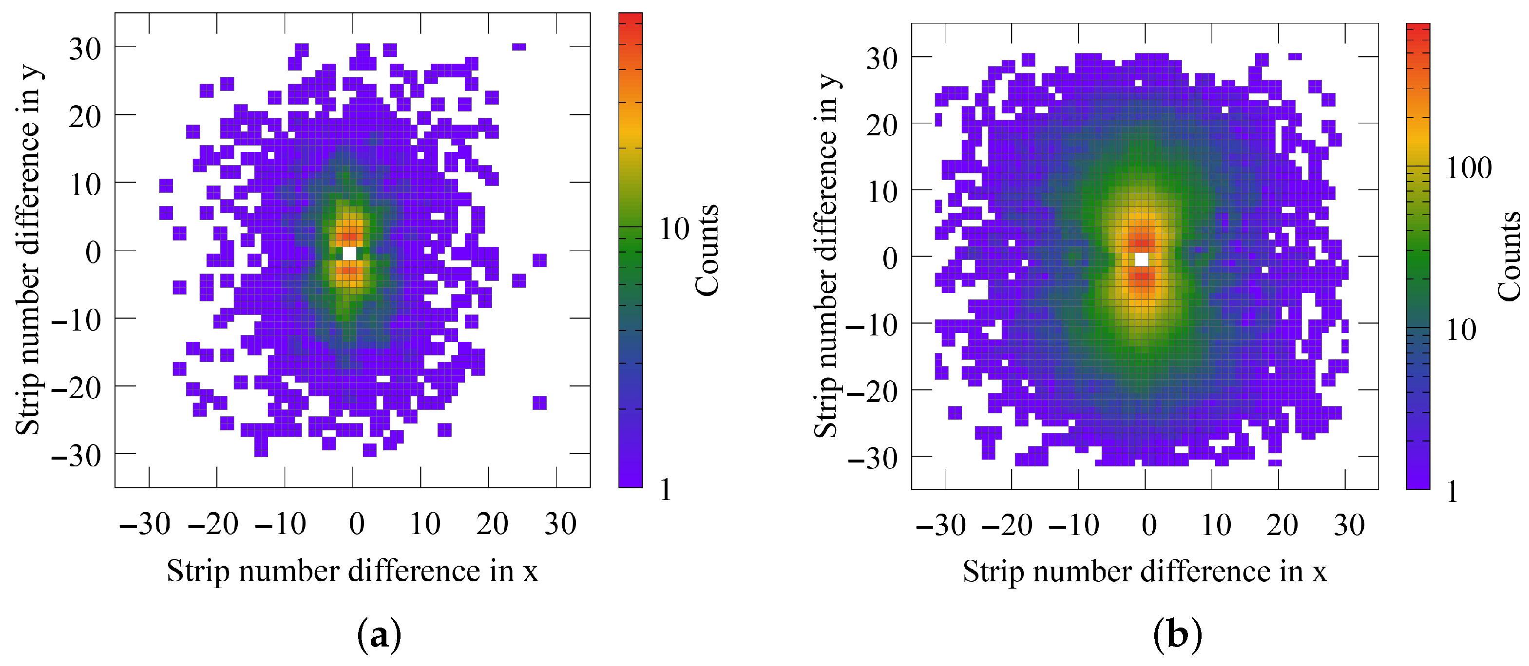
Additionally, we present the result for the radiation being observed within an energy window of $\left(147\pm 1\right) \mathrm{k}\mathrm{e}\mathrm{V}$. For the chosen observation angle of $63.4°$, this energy window corresponds to the center energy of the Compton peak, meaning the radiation being inelastically scattered off the gold target. The 2D scattering distribution of the detector crystal results from Compton scattering events on the detector crystal, where the incident photons were previously also Compton-scattered from the gold target within the set energy window, as well as the reconstruction of the experimental data, as can be seen in Figure 4. Note that we have two subsequent Compton scattering events: the first is the scattering of the gold targets; the scattered radiation will be analyzed upon polarization by the second scattering event, which is Compton scattering on the detector crystal.

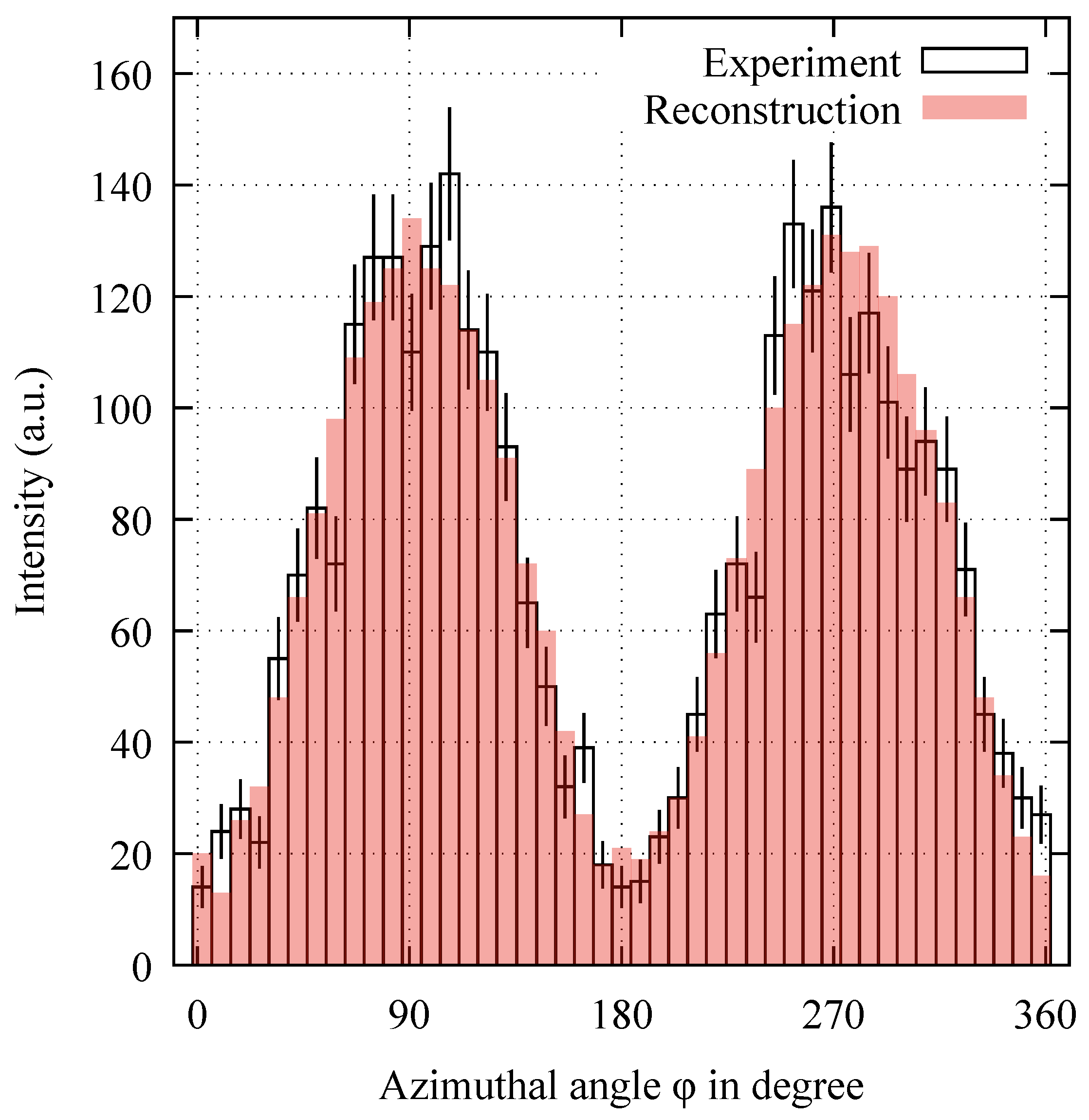
In this representation, for each Compton event, the Compton scattering on the detector crystal is located at the origin. The individual Compton events are therefore shown as the relative distance of the subsequent photoabsorption from the scattering center. Through integrating the counts of Figure 4a, located along a straight line from the center of scattering, the azimuthal scattering distribution (Figure 5) can be generated. Note that, for a better visualization, the azimuthal scattering distribution is corrected by an isotropic distribution to reduce detector effects.

Furthermore, Figure 4b and the red-shaded curve in Figure 5 show the reconstruction of the experimental scattering distribution, which is normalized to the magnitude of the experimental distribution, displayed in Figure 4a and Figure 5, respectively, using the model function in Equation (4). As can be seen, a good agreement between the experimental and reconstructed scattering distribution was reached. From our new algorithm, we reconstructed a degree of polarization of $P_L=0.899\pm 0.028$ and a polarization angle of $\chi =2.9\pm 1.3$ for the photon beam, which Compton scattered off the gold foil at an observation angle of 63.4°. From a calculation of the Compton scattering process based on the transfer matrix method [23], we would expect the scattered photon beam to be linearly polarized with $P_{L,th}=0.879\pm 0.029$ and ${\chi }_{th}=1.5\pm 3.7$. Thus, for this example, the reconstruction algorithm also yields good results compared to the expected values.

7. Conclusions

We briefly explained the technique of Compton polarimetry and presented a state-of-the-art Compton polarimeter setup based on a double-sided segmented semiconductor crystal. This kind of detector can be applied for the efficient determination of the linear polarization of hard X-rays, which are emitted in a lot of fundamental interaction processes. For this detector setup, we presented a new polarization reconstruction algorithm based solely on Monte Carlo-simulated azimuthal scattering distributions on the detector crystal. The model function is build from a linear combination of these simulated data sets. We tested the reconstruction algorithm with the simulated test polarization states, finding good agreement between the test state and reconstruction. Additionally we tested the routine on experimental data, which also showed good consistency. For real data, an additional correction of random double hits was introduced. We expect this polarization reconstruction to provide a good alternative to the already existing method, which is based on an adjustment of the Klein–Nishina formula to an experimental data set and relies on additional corrections by simulated isotropic scattering distribution [19,21]. As the Klein–Nishina formula treats the electrons as free, binding effects (especially the electron momentum distribution) were not considered in the evaluation of the experimental scattering distribution in the previous reconstruction method. On the other hand, the simulation generating the model of azimuthal scattering distribution treats the Compton scattering on the detector crystal within the impulse approximation [31], and thus explicitly considers the scattering of bound electrons. Additionally, the previously necessary pre- and post-processing corrections due to detector properties is now no longer required, as we directly simulated our detector. Moreover, we plan to further improve this reconstruction algorithm. Based on the simulated scattering distributions, not only is an adjustment to the azimuthal scattering distributions possible, but an evaluation of the 3D-resolved $\theta$–$\phi$ scattering distribution can also be performed. This will probably improve the accuracy of the polarization reconstruction as more information will become available due to the inclusion of both the polar and azimuthal scattering angle and because the accepted scattering events do not need to be reduced to polar scattering angles of $\theta =(90°\pm 15°)$, providing more usable scattering events.

In a recent experiment, hard X-rays were scattered off a gold target [29]. The presented reconstruction algorithm was used to determine the linear polarization of the scattered radiation. The publication of the polarization analysis is pending. This routine will be used in future experiments to analyze the polarization of atomic emission and scattering processes for energies beyond $200 \mathrm{k}\mathrm{e}\mathrm{V}$. This will be realized with our novel Compton telescope, which is in the commissioning phase [15].