Effects of Coupling Constants on Chaos of Charged Particles in the Einstein–Æther Theory

Abstract

There are two free coupling parameters $c_{13}$ and $c_{14}$ in the Einstein–Æther metric describing a non-rotating black hole. This metric is the Reissner–Nordström black hole solution when $0\le 2c_{13}<c_{14}<2$, but it is not for $0\le c_{14}<2c_{13}<2$. When the black hole is immersed in an external asymptotically uniform magnetic field, the Hamiltonian system describing the motion of charged particles around the black hole is not integrable; however, the Hamiltonian allows for the construction of explicit symplectic integrators. The proposed fourth-order explicit symplectic scheme is used to investigate the dynamics of charged particles because it exhibits excellent long-term performance in conserving the Hamiltonian. No universal rule can be given to the dependence of regular and chaotic dynamics on varying one or two parameters $c_{13}$ and $c_{14}$ in the two cases of $0\le 2c_{13}<c_{14}<2$ and $0\le c_{14}<2c_{13}<2$. The distributions of order and chaos in the binary parameter space $(c_{13},c_{14})$ rely on different combinations of the other parameters and the initial conditions.

1. Introduction

Detections of gravitational waves [1] and event-horizon-scale images of M87* [2] have strongly supported the prediction of Einstein’s general theory of relativity on the existence of black holes. Although the standard general relativity has attained great success, its extension and development are still necessary because of its limits. One example is that the dark universe beyond the Einstein’s theory may provide a good explanation for the apparent accelerating expansion of the Universe. Another example is the difficulty of building a complete theory unifying interactions and particles in the general relativity and quantum mechanics. Such theories of gravity are called as extended, alternative, or modified gravitational theories.

There are numerous modified gravitational theories in the literature. Some of them are scalar-tensor theories of gravity [3,4], scalar-tensor-vector theories [5,6], Hořava–Lifschitz gravity [7], Kaluza–Klein theories of gravity [8,9], $F\left(R\right)$ gravity [10], quantum field theory in curved spacetime [7,11], and Einstein–Æther theories [12,13,14]. As far as the Einstein–Æther theories are concerned, they are obtained by coupling the Æther field with other fields, such as an electromagnetic field. They violate the Lorentz invariance that is one of the fundamental principles of Einstein’s general relativity. The so-called Æther means the presence of Lorentz-violating vector fields. This particular property can dramatically affect cosmology, and can even affect the growth rate of structure in the Universe. See [15,16,17] for more information on these modified gravitational theories.

From the astrophysical perspective, it is interesting to study the motion of test particles around a black hole in the standard general relativity or a certain modified theory of gravity. The radiation emission by the particles with high energies in the accretion disk leads to the electromagnetic spectrum of astrophysical black hole. The spectrum is useful to understand the effects of Doppler and gravitational red-shift. Circular orbits and the innermost stable circular orbits (ISCOs) of the particles near the black hole can give some important astrophysical information on the nearby activity of the black hole. Thus, their studies have appeared in a large number of publications (see, e.g., [18,19,20,21,22,23,24,25,26,27,28]). The study of photon circular orbits also has a crucial application in astrophysics because the existence of photon circular orbits is closely related to the computation of black hole shadows [29,30,31]. When an external asymptotically uniform magnetic field is included in the vicinity of the black hole, the dynamics of electrically charged particles is non-integrable in general, and is even chaotic. In fact, there are lots of works about the presence of chaotic motions of charged particles around black holes (see, e.g., [32,33,34,35,36,37,38,39]). The chaotic charged particle dynamics is helpful for charged particle acceleration along the magnetic field lines [36]. Chaotic photon motions in non-integrable black hole spacetimes also give self-similar fractal structures to the black hole shadows [40,41].

Rayimbaev et al. [14] studied the effects of Einstein–Æther gravity on the dynamics of magnetized particles around a black hole surrounded by an external asymptotically uniform magnetic field in the equatorial plane. They mainly discussed the impacts of varying the free coupling parameters $c_{13}$ and $c_{14}$ of the Einstein–Æther theory on the radii of the ISCOs, the location of circular orbits, the amount of center-of-mass energy and the strength of the magnetic field. Unlike these authors, we consider in the present work how the two coupling parameters affect the dynamics of electrically charged particles in the 3-dimensional space rather than the equatorial plane. In addition, we design explicit symplectic integrators for the Hamiltonian system describing the motion of charged particles near the Einstein–Æther black hole by following the recent works [42,43,44,45,46]. Such symplectic methods that maintain symplectic nature of Hamiltonian dynamics are the most appropriate solvers for studying the long-term evolution of Hamiltonian systems [47]. One of the proposed explicit symplectic integrators combined with chaos indications such as fast Lyapunov indicators (FLIS) [48] is used to explore the dependence of regular and chaotic dynamics on varying one or two parameters $c_{13}$ and $c_{14}$.

The paper is organized as follows. In Section 2, we introduce the Einstein–Æther black hole metric and its corresponding Hamiltonian system. In Section 3, we establish explicit symplectic integrators and investigate the regular and chaotic dynamics of charged particles. Finally, results are summarized in Section 4.

2. Einstein–Æther Black Hole Metric

Based on the action of Einstein–Æther theory, a metric describing a non-rotating black hole [14] is written in the Schwarzschild coordinates $(t,r,\theta ,\phi )$ as

$$\begin{array}{ccc}\hfill d{s}^2& =& g_{\alpha \beta }d{x}^{\alpha }d{x}^{\beta }=-fd{t}^2+f^{-1}d{r}^2+r^2(d{\theta }^2+{sin}^2\theta d{\phi }^2),\hfill \end{array}$$

(1)

$$\begin{array}{ccc}\hfill f\left(r\right)& =& 1-\frac{2M}{r}\left(1+\frac{2c_{13}-c_{14}}{4(1-c_{13})}\frac{M}{r}\right).\hfill \end{array}$$

(2)

In the metric, t is a coordinate time, and M is the mass of the black hole. $c_{13}=c_1+c_3$ and $c_{14}=c_1+c_4$ are two coupling constants of the Einstein-Æther theory. Of course, $c_1$, $c_3$, $c_4$, and the following parameter $c_2$ are still coupling constants. In fact, they are some of the coefficients in the tensor

$$\begin{array}{c}\hfill M_{\mu \nu }^{\alpha \beta }=c_1{g}_{\mu \nu }{g}^{\alpha \beta }+c_2{\delta }_{\mu }^{\alpha }{\delta }_{\nu }^{\beta }+c_3{\delta }_{\nu }^{\alpha }{\delta }_{\mu }^{\beta }-c_4{u}^{\alpha }{u}^{\beta }{g}_{\mu \nu },\end{array}$$

(3)

which determines the Lagrangian of Æther field

$$\begin{array}{c}\hfill \mathcal{L}=-M_{\mu \nu }^{\alpha \beta }\left(D_{\alpha }{u}^{\mu }\right)\left(D_{\beta }{u}^{\nu }\right)+\Lambda (g_{\mu \nu }{u}^{\mu }{u}^{\nu }+1)\end{array}$$

(4)

in the action

$$\begin{array}{c}\hfill S=\frac{1}{16\pi G}\int d^{4}x\sqrt{-g}\left(\mathcal{R}+\mathcal{L}\right).\end{array}$$

(5)

$G=G_N/(1-c_{14}/2)$ is the Æther gravitational constant, where $G_N$ stands for the Newtonian gravitational constant. $D_{\alpha }$ denotes the covariant derivative with respect to $x^{\alpha }$, $\Lambda$ is the Lagrangian multiplier, and $u^{\alpha }$ is the Æther four-velocity. $g=|g_{\mu \nu }|$, and $\mathcal{R}$ is the curvature. The speed of light C and Newton’s constant of gravity $G_N$ are given geometrized units, $C=G_N=1$.

When the coupling constants $c_{13}$ and $c_{14}$ are given different values, Equation (1) represents different spacetimes. Here, three cases are listed. Case (i): if $c_{14}=2c_{13}\ne 2$, Equation (1) is the Schwarzschild metric. Case (ii): when $0\le c_{13}<1$ and $2c_{13}<c_{14}<2$, Equation (1) represents the Reissner–Nordström (RN) black hole with the electric charge

$$\begin{array}{c}\hfill Q=M\sqrt{(c_{14}-2c_{13})/\left[2(1-c_{13})\right]}\end{array}$$

(6)

and two horizons

$$\begin{array}{c}\hfill R_h^{\pm }=M\left(1\pm \sqrt{(2-c_{14})/\left[2(1-c_{13})\right]}\right).\end{array}$$

(7)

Case (iii): if $0\le c_{13}<1$ and $0\le c_{14}<2c_{13}<2$, Equation (1) shows that the black hole with one horizon $R^{+}$ has no electric charge and is not the RN black hole. In the three cases, the coupling constants $c_{13}$ and $c_{14}$ satisfy the constraints $0\le c_{13}<1$ and $0\le c_{14}<2$ from theoretical and observational bounds [14], which correspond to the presence of one or two horizons.

Consider that an external asymptotically uniform magnetic field exists in the vicinity of black hole. This magnetic field is static, axially symmetric, and homogeneous at the spatial infinity, and has its strength $B>0$ at the spatial infinity. It is so weak that it does not affect the spacetime geometry. Based on the Wald’s method, only one non-vanishing component of the electromagnetic four potential was given in Ref. [14] by:

$$\begin{array}{c}\hfill A_{\phi }=\frac{1}{2}B{r}^2{sin}^2\theta .\end{array}$$

(8)

Although such a weak magnetic field exerts a negligible influence on the spacetime geometry, it plays an important role in the motion of a charged test particle with mass m and charge q. The motion is described by the following Hamiltonian

$$\begin{array}{c}\hfill H=\frac{1}{2m}{g}^{\mu \nu }(p_{\mu }-q{A}_{\mu })(p_{\nu }-q{A}_{\nu }),\end{array}$$

(9)

where the momentum $p_{\mu }$ satisfies the condition

$$\begin{array}{c}\hfill {\dot{x}}^{\mu }=\frac{\partial H}{\partial p_{\mu }}=\frac{1}{m}{g}^{\mu \nu }(p_{\nu }-q{A}_{\nu }),\end{array}$$

(10)

or an equivalent form

$$\begin{array}{c}\hfill p_{\mu }=m{g}_{\mu \nu }{\dot{x}}^{\nu }+q{A}_{\mu }.\end{array}$$

(11)

The four-velocity ${\dot{x}}^{\mu }=(\dot{t},\dot{r},\dot{\theta },\dot{\phi })$ is a derivative of coordinate $x^{\mu }$ with respect to the proper time $\tau$.

To simplify the expressions, we adopt dimensionless operations through scale transformations as follows: $t\to tM$, $\tau \to \tau M$, $r\to rM$, $B\to B/M$, $E\to mE$, $p_t\to m{p}_t$, $p_r\to m{p}_r$, $L\to MmL$, $p_{\theta }\to Mm{p}_{\theta }$, $q\to mq$, and $H\to mH$. In this case, m and M as two mass factors are eliminated in the above expressions.

Because the Hamiltonian (9) does not explicitly depend on the coordinates t and $\phi$, $p_t$ and $p_{\phi }$ are constants of motion, which correspond to the energy E and angular momentum L of the particle:

$$\begin{array}{ccc}\hfill p_t& =& -f\dot{t}=-E,\hfill \end{array}$$

(12)

$$\begin{array}{ccc}\hfill p_{\phi }& =& r^2{sin}^2\theta \dot{\phi }+q{A}_{\phi }=L.\hfill \end{array}$$

(13)

The Hamiltonian (9) is rewritten as

$$\begin{array}{ccc}\hfill H& =& T+V,\hfill \end{array}$$

(14)

$$\begin{array}{ccc}\hfill T& =& \frac{p_r^2}{2}-\frac{p_r^2}{r}+\frac{p_{\theta }^2}{2r^2}-\frac{p_r^2(2c_{13}-c_{14})}{4r^2(1-c_{13})},\hfill \end{array}$$

(15)

$$\begin{array}{cc}\hfill V=& \frac{L^2}{2r^2{sin}^2\theta }+\frac{b^2{r}^2}{8}+\frac{bL}{2sin\theta }\hfill \\ & +\frac{E^2{r}^2(1+c_{13})}{2c_{13}-c_{14}+4(1-c_{13})r-2(1-c_{13})r^2},\hfill \end{array}$$

(16)

where $b=Bq$. Noticing that the four-velocity ${\dot{x}}^{\mu }$ always satisfies the relation $g_{\mu \nu }{\dot{x}}^{\mu }{\dot{x}}^{\nu }=-1$ for a timelike geodesic, we have a third motion constant:

$$\begin{array}{c}\hfill H=-\frac{1}{2}.\end{array}$$

(17)

3. Numerical Simulations

At first, we introduce how to design explicit symplectic integrators for the Hamiltonian (14). Then, an appropriate one of the integrators is used to study the regular and chaotic dynamics of charged particles near the black hole.

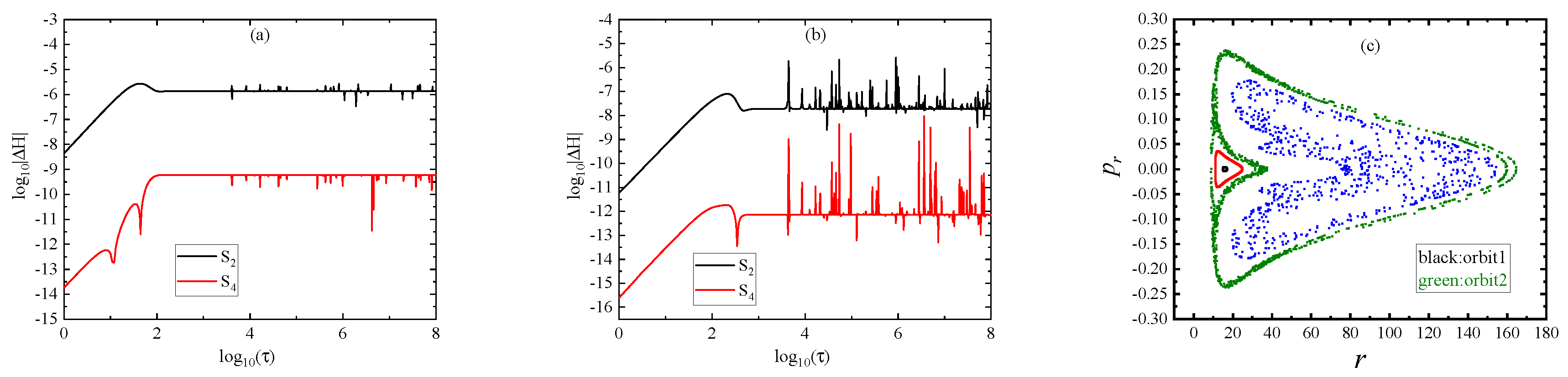
3.1. Explicit Symplectic Integrations

As the authors of [43] claimed, the Hamiltonian (14) can be split into five parts

$$\begin{array}{c}\hfill H=H_1+H_2+H_3+H_4+H_5\end{array}$$

(18)

where these sub-Hamiltonian systems are:

$$\begin{array}{ccc}\hfill H_1& =& V,\hfill \end{array}$$

(19)

$$\begin{array}{ccc}\hfill H_2& =& \frac{p_r^2}{2},\hfill \end{array}$$

(20)

$$\begin{array}{ccc}\hfill H_3& =& -\frac{p_r^2}{r},\hfill \end{array}$$

(21)

$$\begin{array}{ccc}\hfill H_4& =& \frac{p_{\theta }^2}{2r^2},\hfill \end{array}$$

(22)

$$\begin{array}{ccc}\hfill H_5& =& \frac{p_r^2(c_{14}-2c_{13})}{4r^2(1-c_{13})}.\hfill \end{array}$$

(23)

The five splitting parts are solved analytically and their analytical solutions are explicit functions of the proper $\tau$. Operators for analytically solving these sub-Hamiltonians are ${\mathcal{H}}_1$, ${\mathcal{H}}_2$, ${\mathcal{H}}_3$, ${\mathcal{H}}_4$, and ${\mathcal{H}}_5$ in turn. The five-splitting-part method is based on the exclusion of Case (i) with $c_{14}=2c_{13}$.

Setting h as a time step, we have a second-order explicit symplectic algorithm for the Hamiltonian (14)

$$\begin{array}{ccc}\hfill S_2\left(h\right)& =& {\mathcal{H}}_5\left(\frac{h}{2}\right)\times {\mathcal{H}}_4\left(\frac{h}{2}\right)\times {\mathcal{H}}_3\left(\frac{h}{2}\right)\times {\mathcal{H}}_2\left(\frac{h}{2}\right)\times {\mathcal{H}}_1\left(h\right)\hfill \\ & & \times {\mathcal{H}}_2\left(\frac{h}{2}\right)\times {\mathcal{H}}_3\left(\frac{h}{2}\right)\times {\mathcal{H}}_4\left(\frac{h}{2}\right)\times {\mathcal{H}}_5\left(\frac{h}{2}\right).\hfill \end{array}$$

(24)

In such a construction, the sub-Hamiltonian $H_5$ is integrated by advancing the time $h/2$. When the obtained solutions are taken as the initial conditions, we solve the sub-Hamiltonian $H_4$ by advancing the time $h/2$. The operation is also applied to the sub-Hamiltonians $H_3$ and $H_2$. Taking the numerical solutions at the time as the initial conditions, we work out the sub-Hamiltonian $H_1$ by advancing the time h. Then, we continue to solve the sub-Hamiltonian $H_2$, $H_3$, $H_4$, and $H_5$ in sequence by advancing the time $h/2$. As a result, the numerical solutions are outputted in one integration step.

According to the idea of Yoshida [49], the second-order explicit symplectic integrator can be risen to a fourth-order algorithm

$$\begin{array}{c}\hfill S_4=S_2\left(\gamma h\right)\times S_2\left(\delta h\right)\times S_2\left(\gamma h\right),\end{array}$$

(25)

where $\gamma =1/(2-\sqrt[3]{2})$ and $\delta =1-2\gamma$. This construction is explained as follows. We use the algorithm $S_2$ to act on the Hamiltonian (18) by advancing the time $\gamma h$. Taking the numerical solutions as the initial conditions, we continue to solve the Hamiltonian (18) by using the algorithm $S_2$ in a span of time $\delta h$. Finally, we repeat to use the algorithm $S_2$ to integrate the Hamiltonian (18) by advancing the time $\gamma h$. In this way, $\gamma h+\delta h+\gamma h=h$; that is, one step computation finishes.

In our numerical tests, the fixed proper time step $h=1$ is used. The parameters are given by $E=0.995$, $L=4.7$, and $b=9.1\times {10}^{-4}$. The coupling constants are taken as $c_{13}=0.01$ and $c_{14}=0.03$. The initial conditions are $p_r=0$ and $\theta =\pi /2$. Given the initial separation r, the initial value of $p_{\theta }(>0)$ is determined in terms of Equations (14)–(17). The initial separations are $r=15$ for Orbit 1 and $r=35$ for Orbit 2. When the two orbits are integrated by the second-order method $S_2$ and the fourth-order method $S_4$, Hamiltonian errors $\Delta H=H+1/2$ are plotted in Figure 1a,b. These errors show no secular drift with time. This property is an advantage of symplectic integrators. Of course, the errors are sensitive dependence on the step choice. They decrease with a decrease in the time step. However, extremely small steps are not permitted due to the increase in computational cost and the rapid accumulation of round-off errors. Relatively large steps are not, either, because they lead to large errors and make the algorithms unstable. The time step $h=1$ is an appropriate choice in the present problem. Clearly, $S_4$ is superior to $S_2$ in accuracy. Thus, it will be employed in the later computations.

In fact, Orbit 1 is regular and Orbit 2 is chaotic. The regularity or chaoticity is seen from the Poincaré map in the two-dimensional $r-p_r$ plane in Figure 1c. All points in the two-dimensional plane are intersections of the particles’ trajectories with the surface of section $\theta =\pi /2$ with $p_{\theta }>0$ in phase space. The regular dynamics of Orbit 1 is shown because the points in the surface of section form a closed curve, which corresponds to a cross section of a torus in the phase space. The chaotic dynamics of Orbit 2 is known by the points that are distributed randomly in the Poincaré map. The Poincaré map method is a good description of the regular and chaotical dynamical structure of trajectories in a conservative four-dimensional phase space. The algorithms $S_2$ and $S_4$ exhibit good long-term performance in the conservation of the Hamiltonian (14) or (18), irrespective of whether or not the integrated orbit is chaotic.

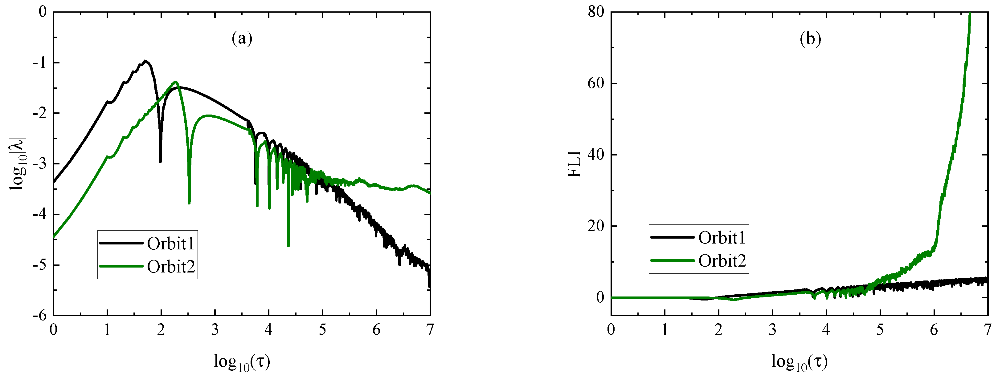
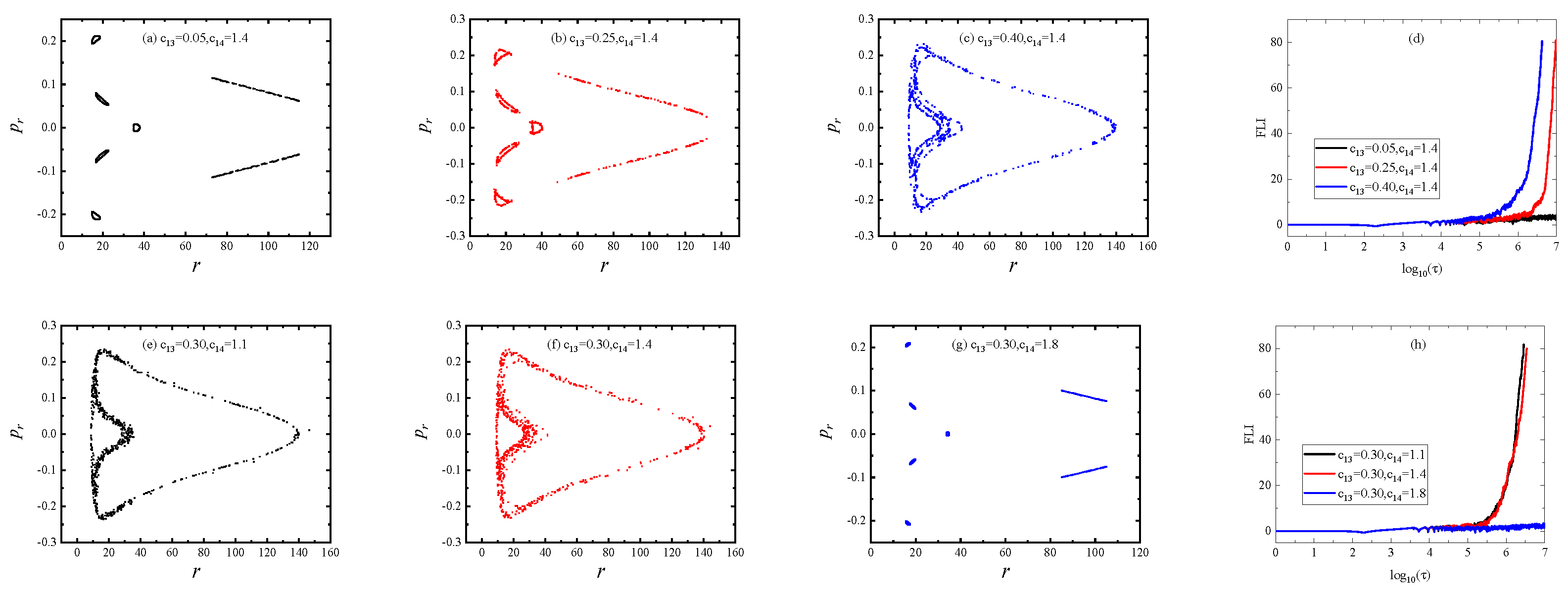
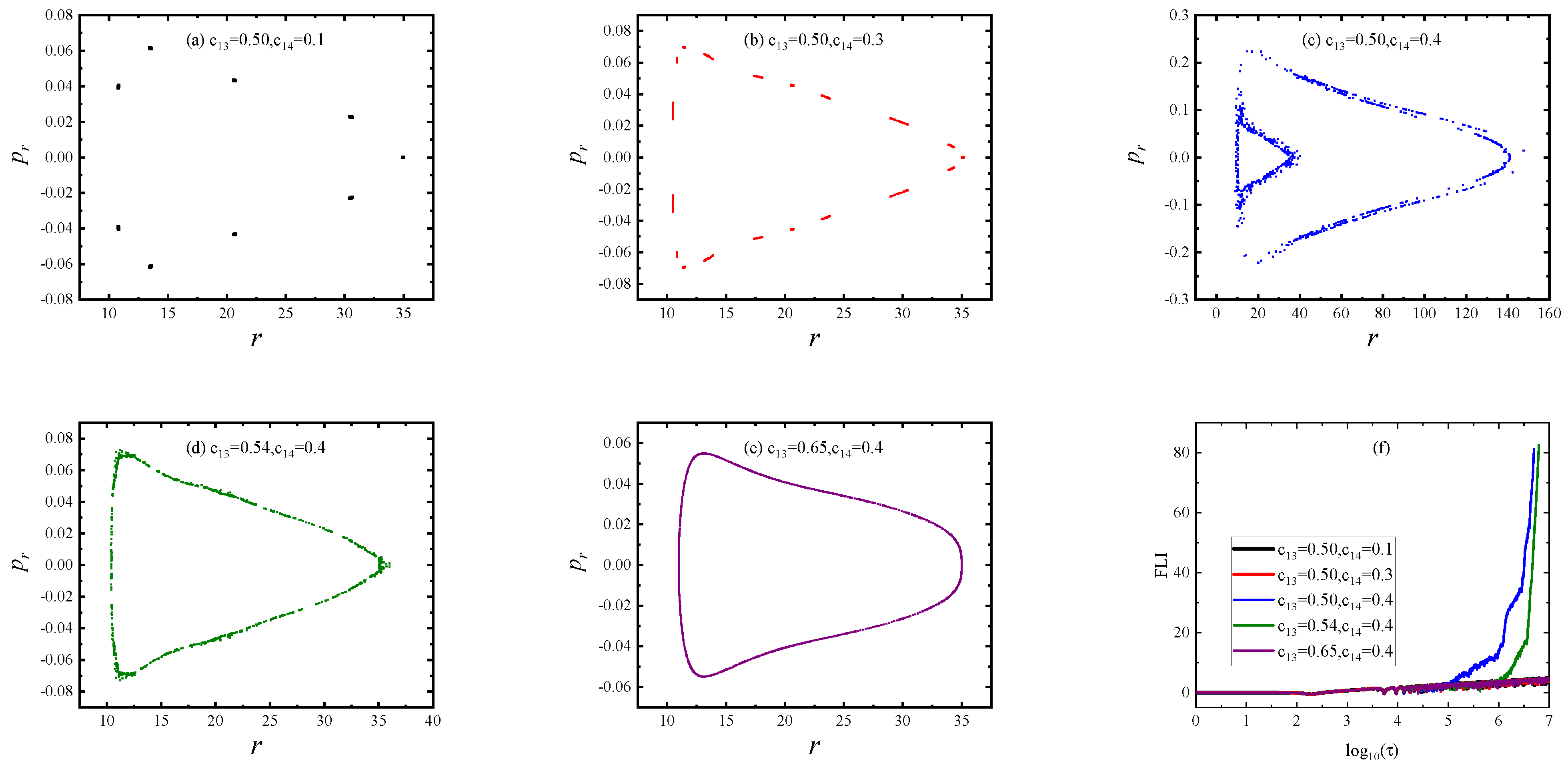
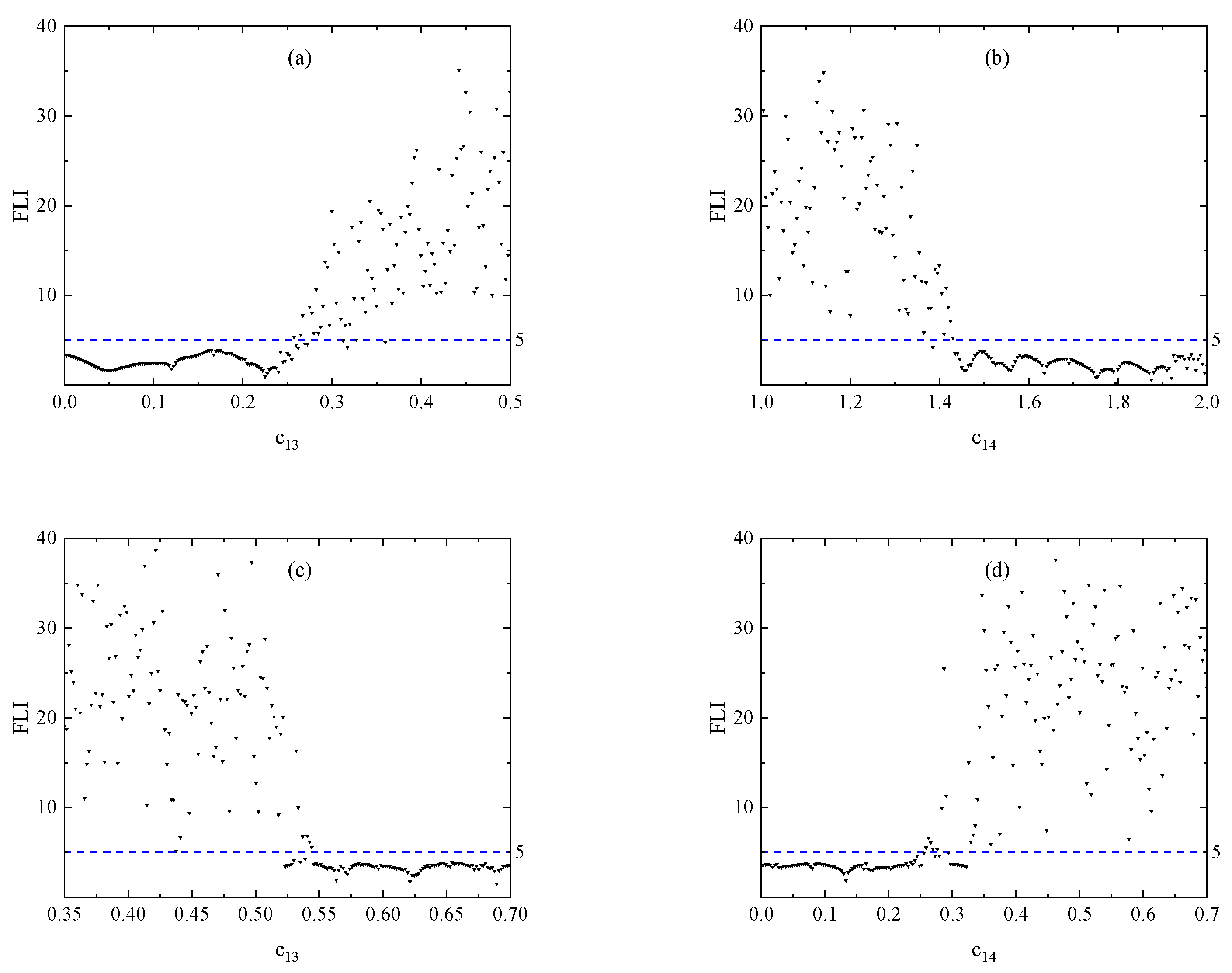
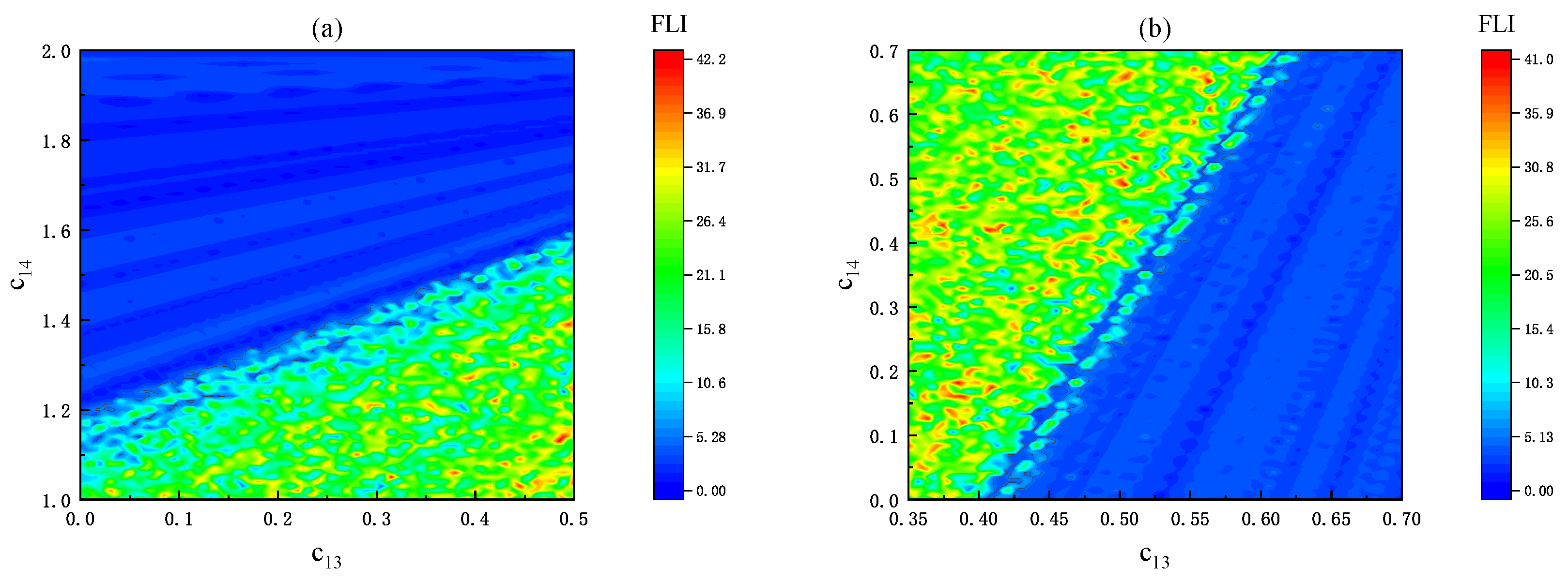
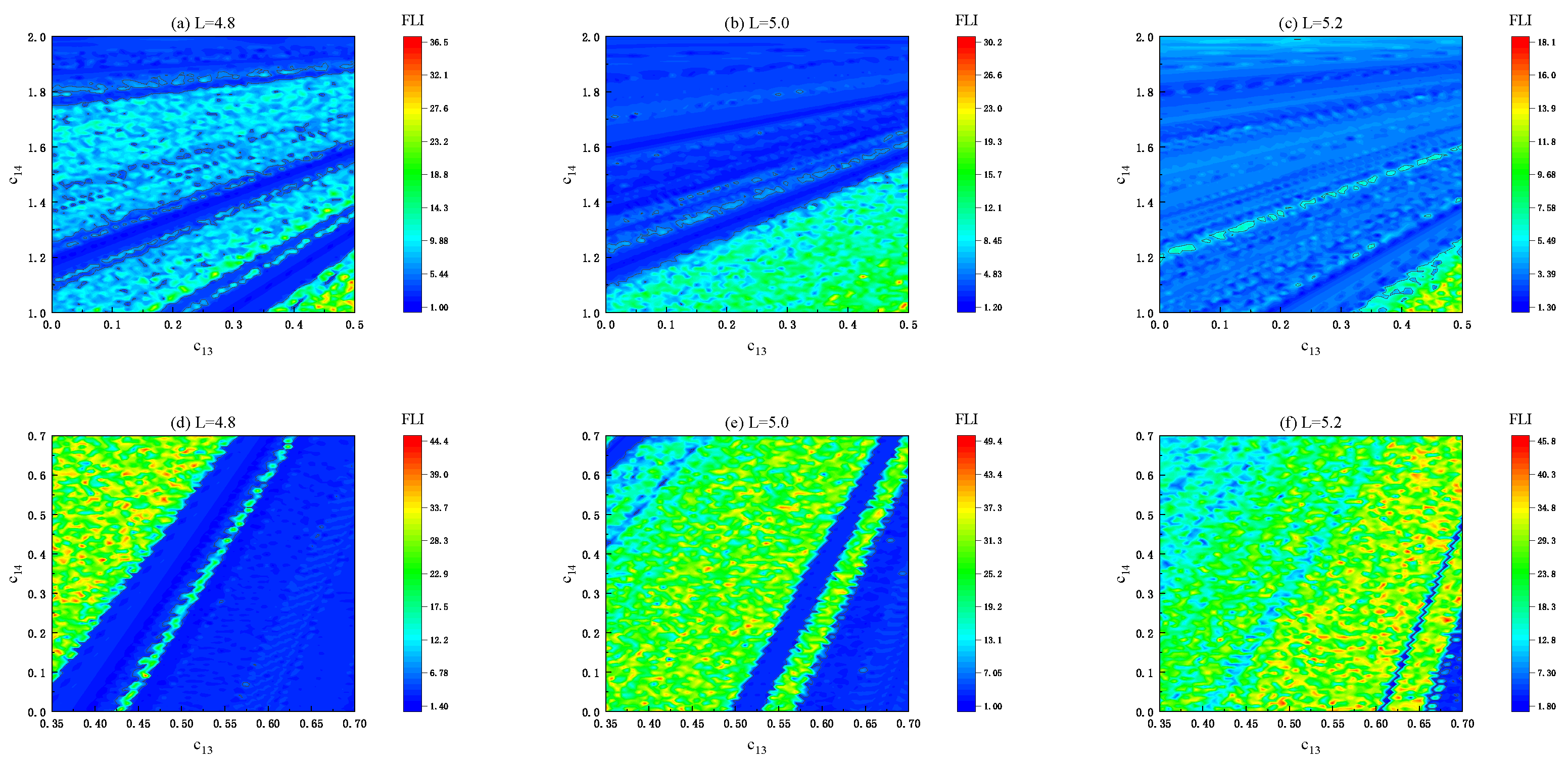
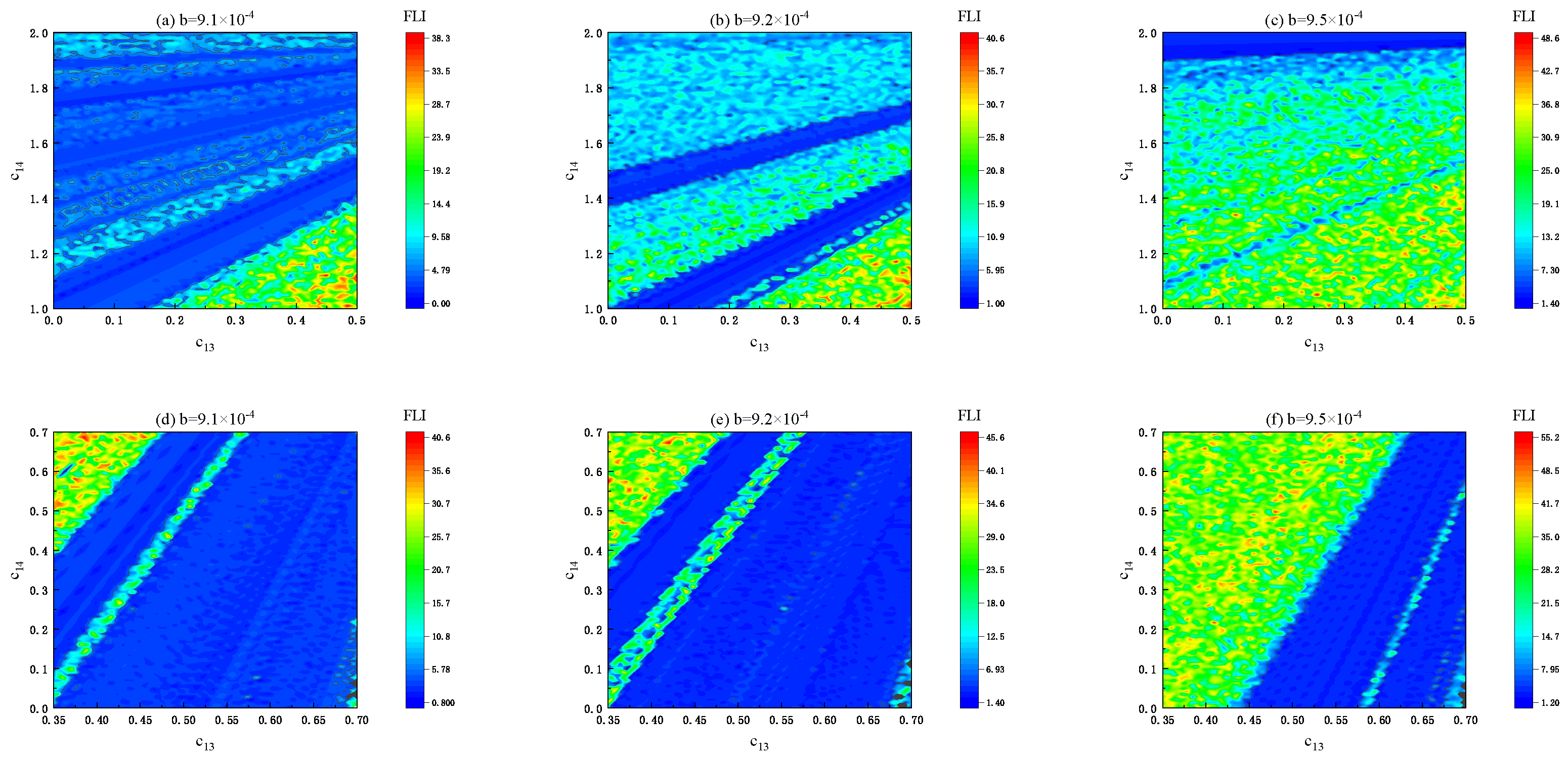
3.2. Orbital Dynamics

In addition to the Poincaré map method, Lyapunov exponents and fast Lyapunov indicators (FLIs) are common methods to detect chaos from order. The maximal Lyapunov exponent corresponding to the most unstable direction in the phase space directly measures how the given orbit is sensitive dependence on the initial conditions. It is defined in [50] as an invariant indicator of chaos under spacetime coordinate transformations within the relativistic framework

$$\begin{array}{c}\hfill \lambda ={\displaystyle \underset{\tau \to \infty }{lim}}ln\frac{1}{\tau }\frac{d\left(\tau \right)}{d\left(0\right)},\end{array}$$

(26)

where $d\left(\tau \right)$ and $d\left(0\right)$ are the proper distances of two nearby orbits at the proper time $\tau$ and the starting time, respectively. $\lambda$ tends to zero for a bounded, regular orbit, while it attains a positive value for a bounded, chaotic orbit. The distinct evolution tendency of $\lambda$ can distinguish between chaotic and regular orbits. Based on this point, the regular dynamics of Orbit 1 and the chaotic dynamics of Orbit 2 are confirmed by the maximal Lyapunov exponents in Figure 2a. The FLI is a quicker method to detect chaos and quasiperiodicity than the largest Lyapunov exponent. Its invariant definition [51] is:

$$\begin{array}{c}\hfill FLI={log}_{10}\frac{d\left(\tau \right)}{d\left(0\right)}.\end{array}$$

(27)

If a bounded orbit has an exponentially increasing FLI with time ${log}_{10}\tau$, it is chaotic. When a bounded orbit has an algebraically increasing FLI, it is ordered. The different deviation of two adjacent orbits with time is used to distinguish between chaotic and regular dynamics. The FLIs in Figure 2b also describe different dynamical behaviors of Orbits 1 and 2.

In what follows, we use the methods of FLIs and Poincaré map to trace the influences of the coupling constants $c_{13}$ and $c_{14}$ on the transition from regular to chaotic dynamics. This consideration is based on Case (ii) with $0\le 2c_{13}<c_{14}<2$ and Case (iii) with $0\le c_{14}<2c_{13}<2$.

In fact, the coupling constants $c_{13}$ and $c_{14}$ considered in Figure 1 correspond to one of the RN type black holes in Case (ii) with $0\le 2c_{13}<c_{14}<2$. In this case, we continue our numerical simulations by taking the parameters $b=9.7\times {10}^{-4}$, $E=0.994$ and $L=4.6$ with the initial separation $r=35$. Given $c_{14}=1.4$, the values of $c_{13}=$ 0.05, 0.25, and 0.40 correspond to the existence of order, weak chaos and strong chaos in Figure 3a–c. Although the orbits seem to be seven-island orbits for $c_{13}=0.05$ and 0.25 from the Poincaré map, $c_{13}=0.05$ indicates the regular dynamics and $c_{13}=0.25$ yields the chaotic dynamics from the FLIs in Figure 3d. These facts seem to show that the transition from regular to chaotic dynamics occurs easily and chaos becomes stronger as the coupling constant $c_{13}$ increases. On the other hand, an increase in the coupling constant $c_{14}$ seems to suppress the occurrence of chaos and to weaken the extent of chaos when the coupling constant $c_{13}=0.3$ is given in Figure 3e–h.

Figure 4 describes the phase space structures of orbits for several values of $c_{14}$ or $c_{13}$ in Case (iii) with $0\le c_{14}<2c_{13}<2$ corresponding to non-RN black holes, where $b=9.4\times {10}^{-4}$, $E=0.994$, $L=4.8$ and $r=35$. In Figure 4a–c, $c_{14}=0.1$ and $c_{14}=0.3$ yield regular dynamics, but $c_{14}=0.4$ exhibits chaotic dynamics for $c_{13}=0.50$. When $c_{14}=0.4$ is given in Figure 4c–e, $c_{13}=0.50$, 0.54 and 0.65 correspond to strong chaos, weak chaos and order in sequence. This fact can also be seen clearly from the FLIs in Figure 4f.

Figure 5a plots the dependence of the FLI on the coupling parameter $c_{13}$ in Case (ii), where the other parameters and the initial separation are those of Figure 3d. Each FLI is computed until the integration time reaches $1\times {10}^6$; 5 is the threshold of the FLI between chaos and order. That is, all FLIs less than 5 indicate the regularity, whereas those larger than or equal to 5 show the chaoticity. Chaos occurs almost everywhere for $c_{13}>0.2611$ in Figure 5a. On the other hand, there is chaos almost everywhere for $c_{14}<1.4302$ with $c_{13}=0.3$ in Figure 5b. The two cases in Figure 5a,b are considered together in Figure 6a that lists a distribution of order and chaos in the binary parameter space $(c_{13},c_{14})$. The region under the line $c_{14}=0.7767c_{13}+1.1972$ is chaotic almost everywhere, while the region over the line is almost regular. The dynamics in Case (iii) are unlike that in Case (ii). Chaos occurs mainly for $c_{13}<0.5396$ with $c_{14}=0.4$ in Figure 5c, and so does it for $c_{14}>0.2610$ with $c_{13}=0.5$ in Figure 5d. The two cases in Figure 5c,d can be shown together through the distribution of order and chaos in the binary parameter space $(c_{13},c_{14})$ in Figure 6b. The main chaotic region is over the line $c_{14}=3.5155c_{13}-1.4968$, and the ordered region is mainly below the line.

Replacing b, E, and L in Figure 6a with $b=9.1\times {10}^{-4}$, $E=0.995$, and $L=4.8,5.0,5.2$, we give distributions of order and chaos in the binary parameter space $(c_{13},c_{14})$ in Figure 7a–c. Based on Case (ii), the distributions are typically different for distinct values of the angular momentum L. When Case (ii) gives place to Case (iii) in Figure 7d–f, the dependence of chaotic dynamics on $c_{13}$ or $c_{14}$ is varied with the variation of L. The chaotic region is enlarged as the angular momentum L increases. The result is unlike that of Refs. [43,44] on the increase in L weakening the degree of chaos.

Figure 8a–c relates to the distributions of order and chaos for several different values of the magnetic parameter b with $L=4.7$ and $E=0.995$ in Case (ii). The chaotic region increases with the magnetic parameter b increasing. This result is also suitable for the increase in energy E in Figure 9a–c and initial radius r in Figure 10a–c. The distributions of order and chaos for several values of b, E or r in Case (iii) (i.e., Figure 8d–f, Figure 9d–f and Figure 10d–f) are different from those in Case (ii).

4. Conclusions

In short, no universal rule can be given to the dependence of regular and chaotic dynamics on varying one or two parameters, $c_{13}$ and $c_{14}$, in Cases (ii) and (iii). The distributions of order and chaos in the binary parameter space $(c_{13},c_{14})$ are different when different combinations of the other parameters E, L, b, and the initial radius r are considered. This result should be reasonable because not only one or two parameters but also a combination of the other parameters and the initial conditions are responsible for the occurrence of chaos.

The Einstein–Æther gravity is a covariant theory of gravity violating the local Lorentz symmetry. In the Einstein–Æther metric describing a non-rotating black hole, there are two free parameters, $c_{13}$ and $c_{14}$. This metric corresponds to the RN black hole solution when the two free parameters satisfy the condition $0\le 2c_{13}<c_{14}<2$, but it is a non-RN black hole solution for the case of $0\le c_{14}<2c_{13}<2$. The spacetime is integrable in the two cases. When the black hole is immersed in an external asymptotically uniform magnetic field, the dynamic of charged particles moving around the non-rotating black hole is not integrable.

There are five explicitly integrable splitting terms in the Hamiltonian system describing the motion of charged test particles around the Einstein–Æther black hole surrounded by the external magnetic field. This gives a good chance for the construction of explicit symplectic integrators. Numerical tests show that the established second- and fourth-order explicit symplectic methods exhibit excellent long-term performance in accuracy of conserving the Hamiltonian. The fourth-order explicit symplectic scheme is chosen to investigate the dynamics of charged particles.

There is no universal rule for the dependence of regular and chaotic dynamics on varying one or two parameters, $c_{13}$ and $c_{14}$, in the two cases of $0\le 2c_{13}<c_{14}<2$ and $0\le c_{14}<2c_{13}<2$. The distributions of order and chaos in the binary parameter space $(c_{13},c_{14})$ rely on different combination of the other parameters and the initial conditions.

References

1. Abbott, B.P. et al. [LIGO Scientific Collaboration and Virgo Collaboration] Observation of Gravitational Waves from a Binary Black Hole Merger. Phys. Rev. Lett. 2016, 116, 061102. [Google Scholar] [CrossRef] [PubMed] [Green Version]
2. Akiyama, K. et al. [The Event Horizon Telescope Collaboration] First M87 Event Horizon Telescope Results. I. The Shadow of the Supermassive Black Hole. Astrophys. J. Lett. 2019, 875, L1. [Google Scholar]
3. Wagoner, R.V. Scalar tensor theory and gravitational waves. Phys. Rev. D 1970, 1, 3209–3216. [Google Scholar] [CrossRef]
4. Deng, X.-M.; Xie, Y. Solar System tests of a scalar-tensor gravity with a general potential: Insensitivity of light deflection and Cassini tracking. Phys. Rev. D 2016, 93, 044013. [Google Scholar] [CrossRef]
5. Moffat, J.W. Scalar tensor vector gravity theory. J. Cosmol. Astropart. Phys. 2006, 3, 4. [Google Scholar] [CrossRef] [Green Version]
6. Skordis, C. The tensor-vector-scalar theory and its cosmology. Class. Quantum Gravity 2009, 26, 143001. [Google Scholar] [CrossRef] [Green Version]
7. Horava, P. Spectral Dimension of the Universe in Quantum Gravity at a Lifshitz Point. Phys. Rev. Lett. 2009, 102, 161301. [Google Scholar] [CrossRef] [Green Version]
8. Deng, X.-M.; Xie, Y. Improved upper bounds on Kaluza-Klein gravity with current Solar System experiments and observations. Eur. Phys. J. C 2015, 75, 539. [Google Scholar] [CrossRef] [Green Version]
9. Katore, S.D.; Hatkar, S.P.; Tadas, D.P. Accelerating Kaluza-Klein Universe in Modified Theory of Gravitation. Astrophysics 2023, 66, 98. [Google Scholar] [CrossRef]
10. Sotiriou, T.P.; Faraoni, V. f(R) theories of gravity. Rev. Mod. Phys. 2010, 82, 451. [Google Scholar] [CrossRef] [Green Version]
11. Gao, B.; Deng, X.-M. Dynamics of charged test particles around quantum-corrected Schwarzschild black holes. Eur. Phys. J. C 2021, 81, 983. [Google Scholar] [CrossRef]
12. Jacobson, T.; Mattingly, D. Einstein-æther gravity: A status report. Phys. Rev. D 2001, 64, 024028. [Google Scholar] [CrossRef] [Green Version]
13. Ding, C.; Wang, A.; Wang, X. Charged Einstein-Æther black holes and Smarr formula. Phys. Rev. D 2015, 92, 084055. [Google Scholar] [CrossRef] [Green Version]
14. Rayimbaev, J.; Abdujabbarov, A.; Jamil, M.; Han, W.-B. Dynamics of magnetized particles around Einstein-Æther black hole with uniform magnetic field. Nucl. Phys. B 2021, 966, 115364. [Google Scholar] [CrossRef]
15. Clifton, T.; Ferreira, P.G.; Padilla, A.; Skordis, C. Modified gravity and cosmology. Phys. Rep. 2012, 513, 1–189. [Google Scholar] [CrossRef] [Green Version]
16. Nojiri, S.; Odintsov, S.D. Unified cosmic history in modified gravity: From F(R) theory to Lorentz non-invariant models. Phys. Rep. 2011, 505, 59. [Google Scholar] [CrossRef] [Green Version]
17. Nojiri, S.; Odintsov, S.D.; Oikonomou, V.K. Modified gravity theories on a nutshell: Inflation, bounce and late-time evolution. Phys. Rep. 2017, 692, 1–104. [Google Scholar] [CrossRef] [Green Version]
18. Esteban, E.P.; Medina, I.R. Accretion onto black holes in external magnetic fields. Phys. Rev. D 1990, 42, 307. [Google Scholar] [CrossRef]
19. de Felice, F.; Sorge, F. Magnetized orbits around a Schwarzschild black hole. Class. Quantum Gravity 2003, 20, 469–481. [Google Scholar] [CrossRef]
20. Abdujabbarov, A.; Ahmedov, B.; Rahimov, O.; Salikhbaev, U. Magnetized particle motion and acceleration around a Schwarzschild black hole in a magnetic field. Phys. Scr. 2014, 89, 084008. [Google Scholar] [CrossRef]
21. Kološ, M.; Stuchlík, Z.; Tursunov, A. Quasi-harmonic oscillatory motion of charged particles around a Schwarzschild black hole immersed in a uniform magnetic field. Class. Quantum Gravity 2015, 32, 165009. [Google Scholar] [CrossRef] [Green Version]
22. Shaymatov, S.; Patil, M.; Ahmedov, B.; Joshi, P.S. Destroying a near-extremal Kerr black hole with a charged particle: Can a test magnetic field serve as a cosmic censor? Phys. Rev. D 2015, 91, 064025. [Google Scholar] [CrossRef] [Green Version]
23. Tursunov, A.; Stuchlík, Z.; Kološ, M. Circular orbits and related quasiharmonic oscillatory motion of charged particles around weakly magnetized rotating black holes. Phys. Rev. D 2016, 93, 084012. [Google Scholar] [CrossRef] [Green Version]
24. Lin, H.-Y.; Deng, X.-M. Rational orbits around 4 D Einstein–Lovelock black holes. Phys. Dark Universe 2021, 31, 100745. [Google Scholar] [CrossRef]
25. Gao, B.; Deng, X.-M. Bound orbits around modified Hayward black holes. Mod. Phys. Lett. A 2021, 36, 2150237. [Google Scholar] [CrossRef]
26. Deng, X.-M. Geodesics and periodic orbits around quantum-corrected black holes. Phys. Dark Universe 2020, 30, 100629. [Google Scholar] [CrossRef]
27. Deng, X.-M. Periodic orbits around brane-world black holes. Eur. Phys. J. C 2020, 80, 489. [Google Scholar] [CrossRef]
28. Gao, B.; Deng, X.-M. Bound orbits around Bardeen black holes. Ann. Phys. 2020, 418, 168194. [Google Scholar] [CrossRef]
29. Odintsov, S.D.; Oikonomou, V.K. Dissimilar donuts in the sky? Effects of a pressure singularity on the circular photon orbits and shadow of a cosmological black hole. Europhys. Lett. 2022, 139, 59003. [Google Scholar] [CrossRef]
30. Chakraborty, S. Bound on Photon Circular Orbits in General Relativity and Beyond. Galaxies 2021, 9, 96. [Google Scholar] [CrossRef]
31. Qiao, C.-K.; Li, M. Geometric approach to circular photon orbits and black hole shadows. Phys. Rev. D 2022, 106, L021501. [Google Scholar] [CrossRef]
32. Nakamura, Y.; Ishizuka, T. Motion of a Charged Particle Around a Black Hole Permeated by Magnetic Field and its Chaotic Characters. Astrophys. Space Sci. 1993, 210, 105–108. [Google Scholar] [CrossRef]
33. Takahashi, M.; Koyama, H. Chaotic Motion of Charged Particles in an Electromagnetic Field Surrounding a Rotating Black Hole. Astrophys. J. 2009, 693, 472. [Google Scholar] [CrossRef] [Green Version]
34. Kopáček, O.; Karas, V.; Kovář, J.; Stuchlík, Z. Transition from Regular to Chaotic Circulation in Magnetized Coronae near Compact Objects. Astrophys. J. 2010, 722, 1240. [Google Scholar] [CrossRef]
35. Kopáček, O.; Karas, V. Inducing Chaos by Breaking Axil Symmetry in a Black Hole Magenetosphere. Astrophys. J. 2014, 787, 117. [Google Scholar] [CrossRef] [Green Version]
36. Stuchlík, Z.; Kološ, M. Acceleration of the charged particles due to chaotic scattering in the combined black hole gravitational field and asymptotically uniform magnetic field. Eur. Phys. J. C 2016, 76, 32. [Google Scholar] [CrossRef] [Green Version]
37. Kopáček, O.; Karas, V. Near-horizon Structure of Escape Zones of Electrically Charged Particles around Weakly Magnetized Rotating Black Hole. Astrophys. J. 2018, 853, 53. [Google Scholar] [CrossRef] [Green Version]
38. Pánis, R.; Kološ, M.; Stuchlík, Z. Determination of chaotic behaviour in time series generated by charged particle motion around magnetized Schwarzschild black holes. Eur. Phys. J. C 2019, 79, 479. [Google Scholar] [CrossRef] [Green Version]
39. Stuchlík, Z.; Kološ, M.; Kovář, J.; Tursunov, A. Influence of Cosmic Repulsion and Magnetic Fields on Accretion Disks Rotating around Kerr Black Holes. Universe 2020, 6, 26. [Google Scholar] [CrossRef] [Green Version]
40. Shipley, J.O.; Dolan, S.R. Binary black hole shadows, chaotic scattering and the Cantor set. Class. Quantum Gravity 2016, 33, 175001. [Google Scholar] [CrossRef] [Green Version]
41. Wang, M.; Chen, S.; Wang, J.; Jing, J. Shadow of a Schwarzschild black hole surrounded by a Bach-Weyl ring. Eur. Phys. J. C 2020, 80, 110. [Google Scholar] [CrossRef] [Green Version]
42. Wang, Y.; Sun, W.; Liu, F.; Wu, X. Construction of Explicit Symplectic Integrators in General Relativity. I. Schwarzschild Black Holes. Astrophys. J. 2021, 907, 66. [Google Scholar] [CrossRef]
43. Wang, Y.; Sun, W.; Liu, F.; Wu, X. Construction of Explicit Symplectic Integrators in General Relativity. II. Reissner-Nordström Black Holes. Astrophys. J. 2021, 909, 22. [Google Scholar] [CrossRef]
44. Wang, Y.; Sun, W.; Liu, F.; Wu, X. Construction of Explicit Symplectic Integrators in General Relativity. III. Reissner-Nordström-(anti)-de Sitter Black Holes. Astrophys. J. Suppl. Ser. 2021, 254, 8. [Google Scholar] [CrossRef]
45. Wu, X.; Wang, Y.; Sun, W.; Liu, F. Construction of Explicit Symplectic Integrators in General Relativity. IV. Kerr Black Holes. Astrophys. J. 2021, 914, 63. [Google Scholar] [CrossRef]
46. Wu, X.; Wang, Y.; Sun, W.; Liu, F.-Y.; Han, W.-B. Explicit Symplectic Methods in Black Hole Spacetimes. Astrophys. J. 2022, 940, 166. [Google Scholar] [CrossRef]
47. Yoshida, H. Recent Progress in the Theory and Application of Symplectic Integrators. Celest. Mech. Dyn. Astron. 1993, 56, 27. [Google Scholar] [CrossRef]
48. Froeschlé, C.; Lega, E. On the Structure of Symplectic Mappings. The Fast Lyapunov Indicator: A Very Sensitive Tool. Celest. Mech. Dyn. Astron. 2000, 78, 167. [Google Scholar] [CrossRef]
49. Yoshida, H. Construction of higher order symplectic integrators. Phys. Lett. A 1990, 150, 262. [Google Scholar] [CrossRef]
50. Wu, X.; Huang, T.-Y. Computation of Lyapunov exponents in general relativity. Phys. Lett. A 2003, 313, 77. [Google Scholar] [CrossRef] [Green Version]
51. Wu, X.; Huang, T.-Y.; Zhang, H. Lyapunov indices with two nearby trajectories in a curved spacetime. Phys. Rev. D 2006, 74, 083001. [Google Scholar] [CrossRef] [Green Version]
Figure 1. (a) Hamiltonian errors  Δ H = H + 1 / 2  in Equation (17) for the two sympletic methods  S 1  and  S 4  acting on Orbit 1. (b) Same as (a) but Orbit 1 replaced with Orbit 2. (c) Poincaré map at the plane  θ = π / 2  with  p θ > 0 . The parameters are  E = 0.995 L = 4.7 b = 9.1 × 10 4 q = 1 c 13 = 0.01  and  c 14 = 0.03  in Case (ii); the initial conditions are  p r = 0  and  θ = π / 2 . Orbit 1 with the initial separation  r = 15  is regular, whereas Orbit 2 with the initial separation  r = 35  is chaotic.
Universe 09 00365 g001
Figure 2. (a) The largest Lyapunov exponents  λ  for Orbits 1 and 2. (b) The fast Lyapunov indicators (FLIs) for Orbits 1 and 2.
Universe 09 00365 g002
Figure 3. (ac): Poincaré sections in Case (ii) of  0 2 c 13 < c 14 < 2 . The parameters are  b = 9.7 × 10 4 E = 0.994 L = 4.6 c 14 = 1.4 , and  c 13  is given different values in (ac). The initial radius is  r = 35 . (d): The FLIs for the orbits in (ac). (eh): Same as (ad), but  c 13 = 0.30  is given and  c 14  has distinct values.
Universe 09 00365 g003
Figure 4. (ae): Poincaré sections in Case (iii) of  0 c 14 < 2 c 13 < 2 . The parameters are  b = 9.4 × 10 4 E = 0.994 L = 4.8 ; the initial radius is  r = 35 . In (ac),  c 13 = 0.50 , and  c 14  has different values. In (d,e),  c 14 = 0.40 , and  c 13  has two different values. (f): The FLIs for the orbits in (ae).
Universe 09 00365 g004
Figure 5. Dependence of FLI on  c 13  or  c 14 . (a,b): Corresponding to Figure 3 c 14 = 1.4  is fixed in (a), and  c 13 = 0.3  is fixed in (b). (c,d): Corresponding to Figure 4 c 14 = 0.4  is fixed in (c), and  c 13 = 0.5  is fixed in (d).
Universe 09 00365 g005
Figure 6. Distributions of order and chaos in the two parameter space  ( c 13 , c 14 )  using the FLIs. The initial radius is  r = 35 . (a b = 9.7 × 10 4 E = 0.994  and  L = 4.6  in Case (ii). (b B = 9.4 × 10 4 E = 0.994  and  L = 4.8  in Case (iii).
Universe 09 00365 g006
Figure 7. Same as Figure 6, but several values are given to the angular momentum L. The initial radius is  r = 35 , and the other parameters are  b = 9.1 × 10 4  and  E = 0.995 . (ac): Case (ii) is considered. (df): Case (iii) is considered.
Universe 09 00365 g007
Figure 8. Same as Figure 7, but several values are given to the magnetic field parameter b. The initial radius is  r = 35 , and the other parameters are  L = 4.7  and  E = 0.995 . (ac): Case (ii). (df): Case (iii).
Universe 09 00365 g008
Figure 9. Same as Figure 8, but several values are given to the energy E. The initial radius is  r = 35 , and the other parameters are  b = 9.5 × 10 4  and  L = 4.7 . (ac): Case (ii). (df): Case (iii).
Universe 09 00365 g009
Figure 10. Same as Figure 9, but several values are given to the initial radius r. The other parameters are  b = 9.1 × 10 4 E = 0.995  and  L = 4.7 . (ac): Case (ii). (df): Case (iii).
Universe 09 00365 g010
Disclaimer/Publisher’s Note: The statements, opinions and data contained in all publications are solely those of the individual author(s) and contributor(s) and not of MDPI and/or the editor(s). MDPI and/or the editor(s) disclaim responsibility for any injury to people or property resulting from any ideas, methods, instructions or products referred to in the content.