
Analysis of Resonant Periodic Orbits in the Framework of the Perturbed Restricted Three Bodies Problem


Abstract
1. Introduction
- Alpha Eridani is Achernar’s closest neighbour. It is also known as “Achernar B” is an oblate star that orbit around Achernar as part of a binary system.
- Zaurak also known as Gamma Eridani is another oblate star located near Achernar.
2. Perturbed Forces
2.1. Radiation Perturbed Forces
2.2. Oblateness Effect
3. Mean Motion of Two Oblate Bodies
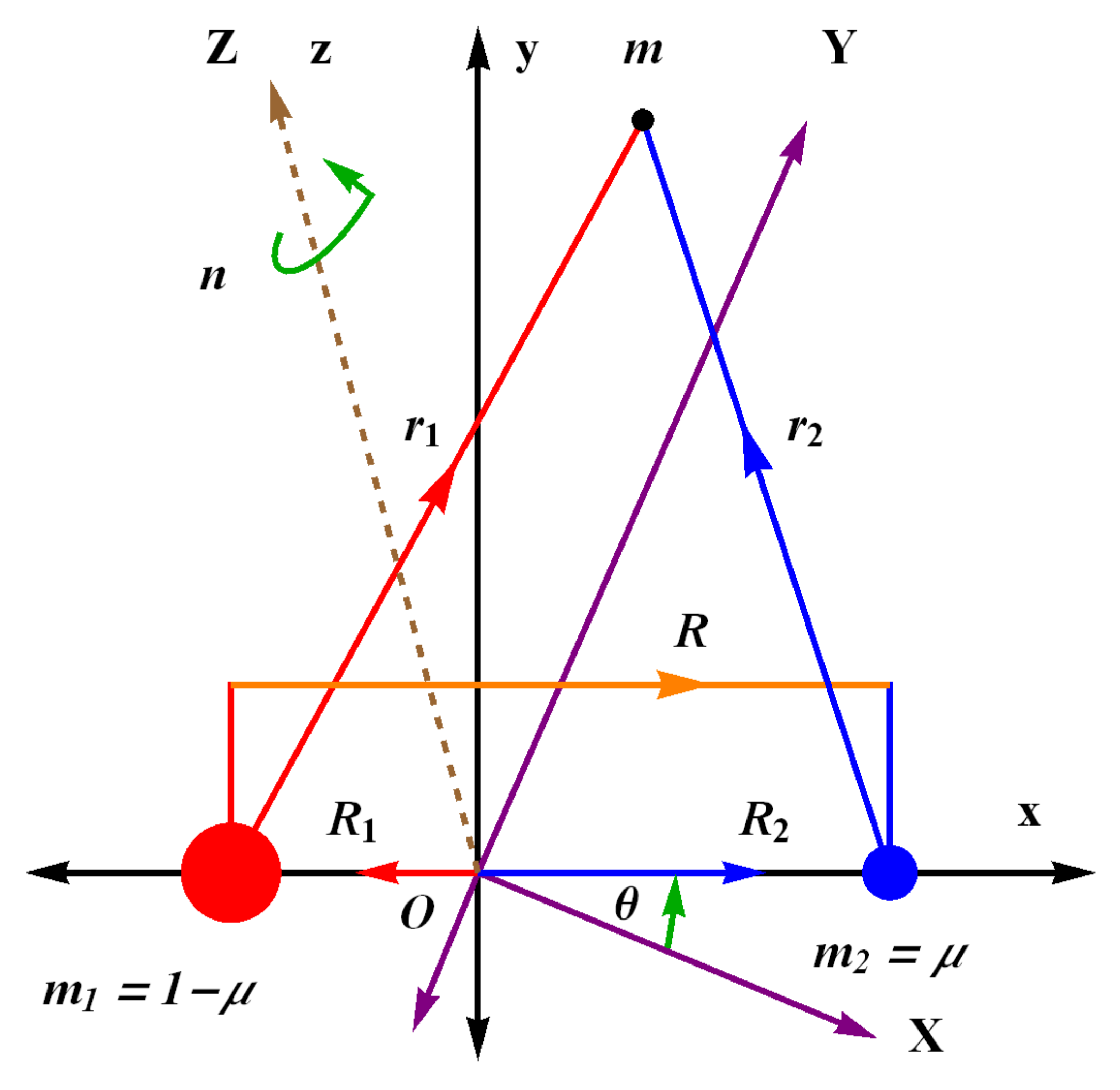
4. Model Description
5. Computation of Collinear Lagrange Points
- Location of
- Location of
- Location of
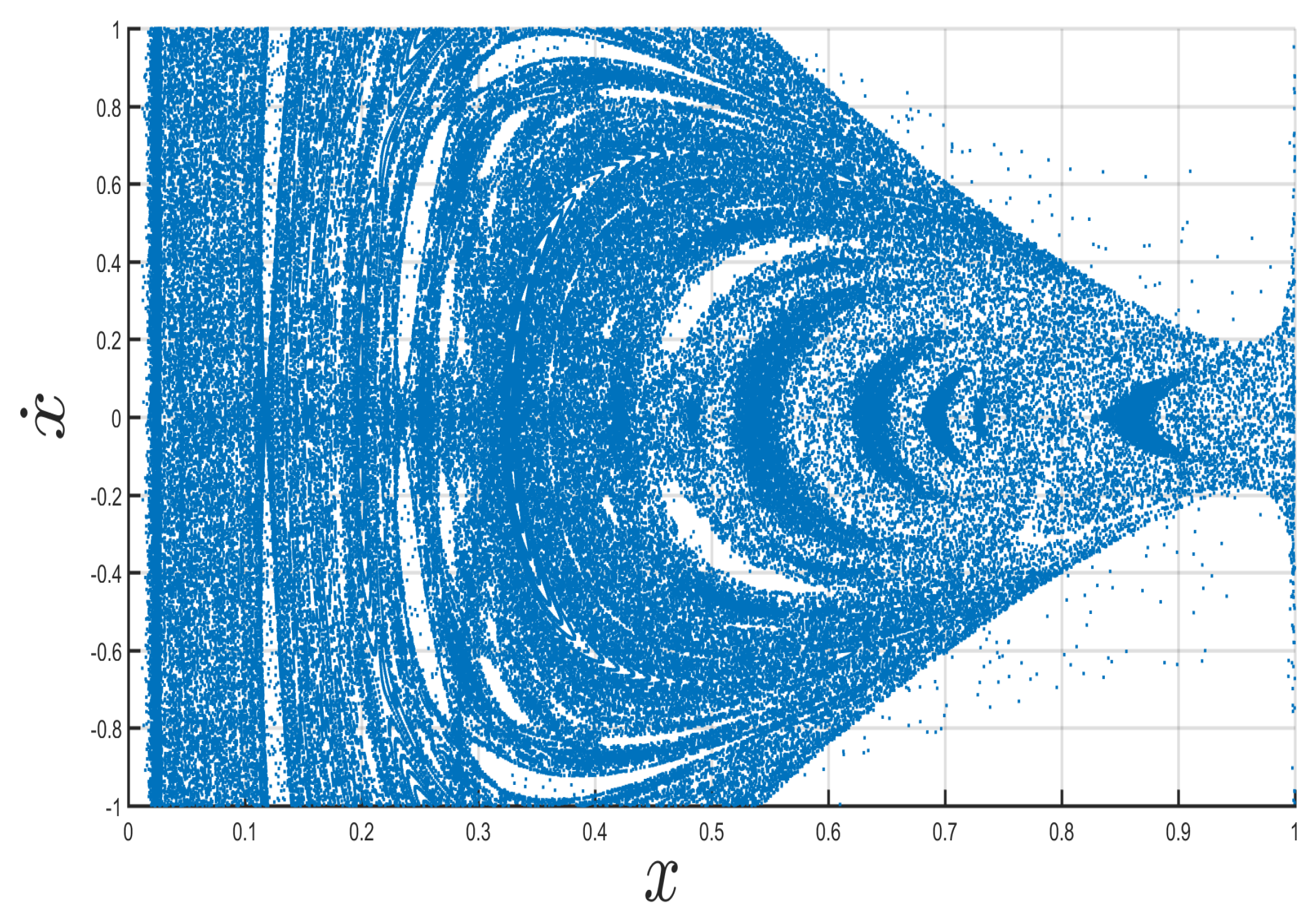
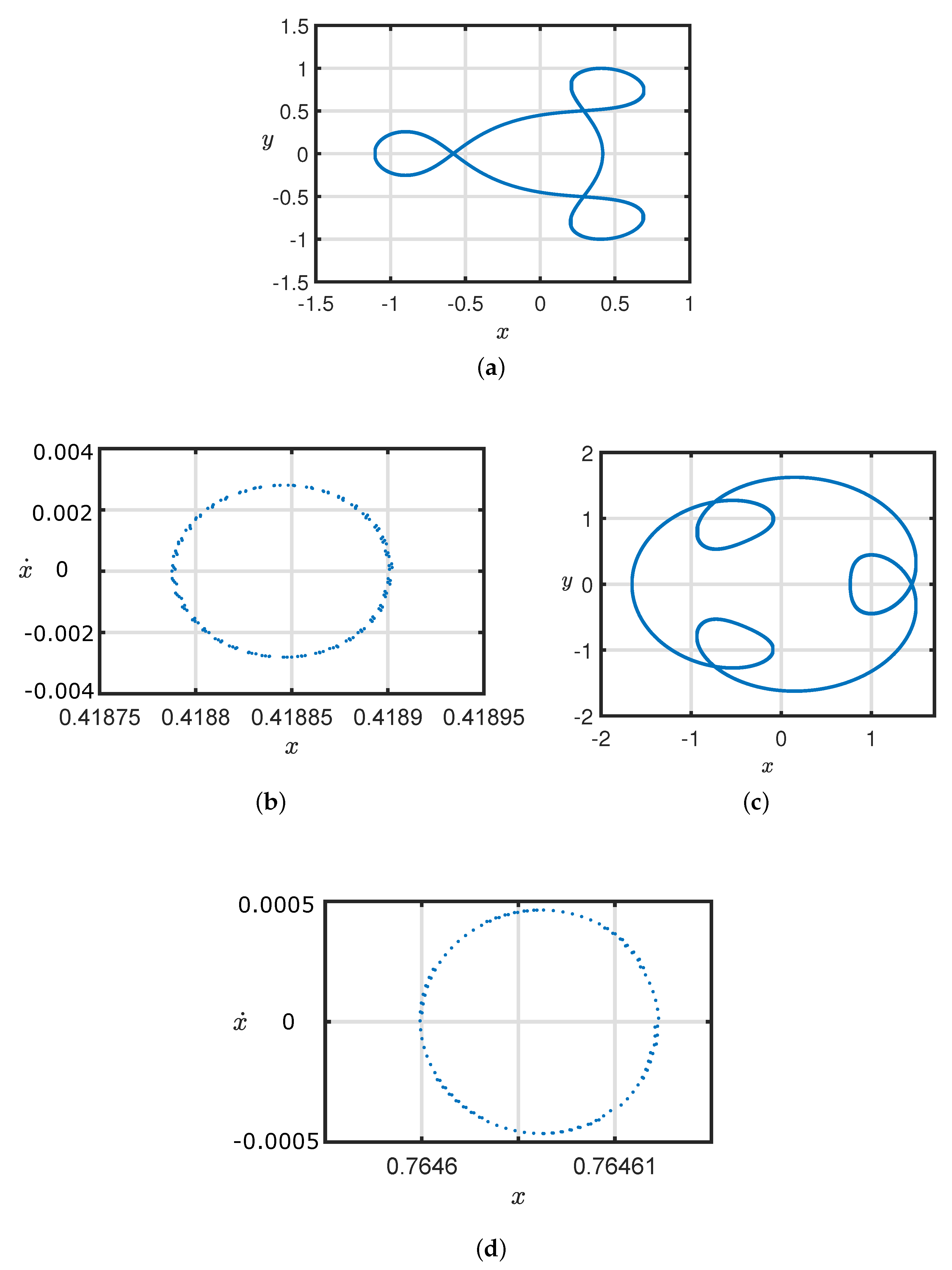
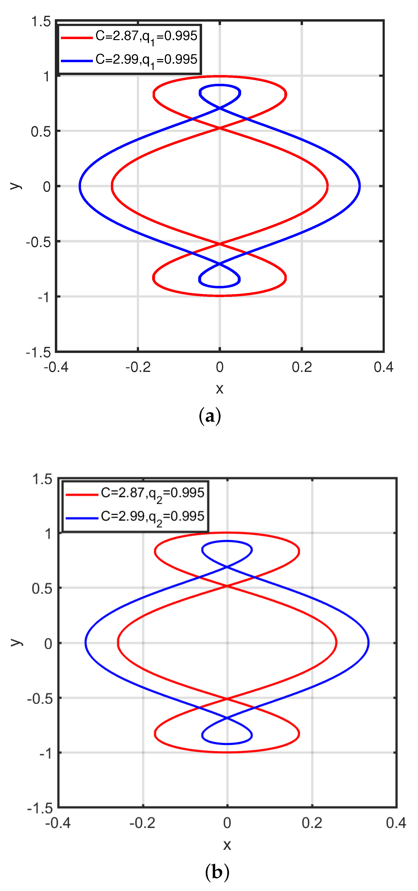
6. Resonant Periodic Orbits
7. Numerical Analysis of Periodic Orbits
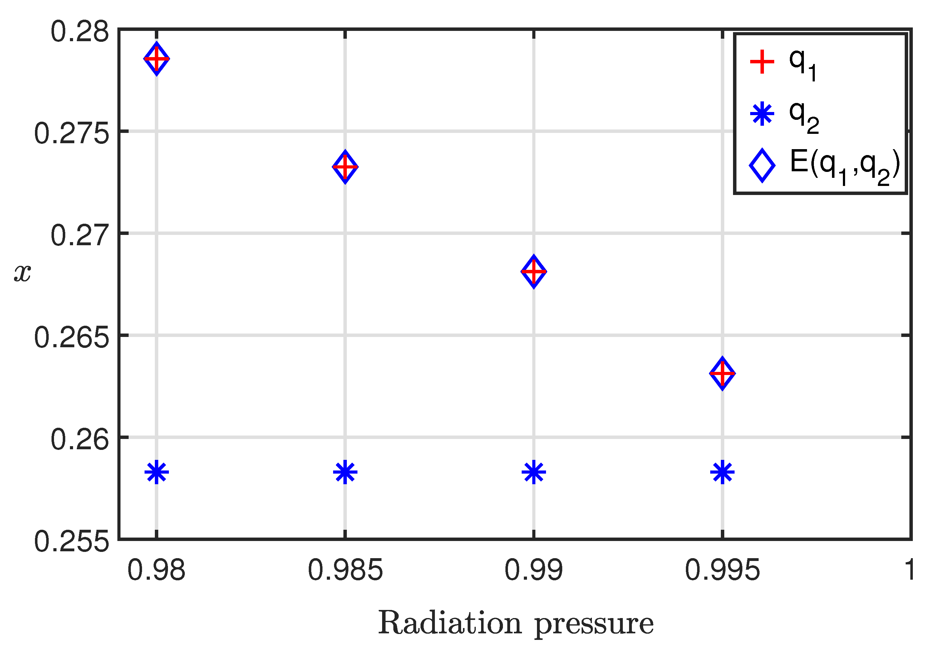
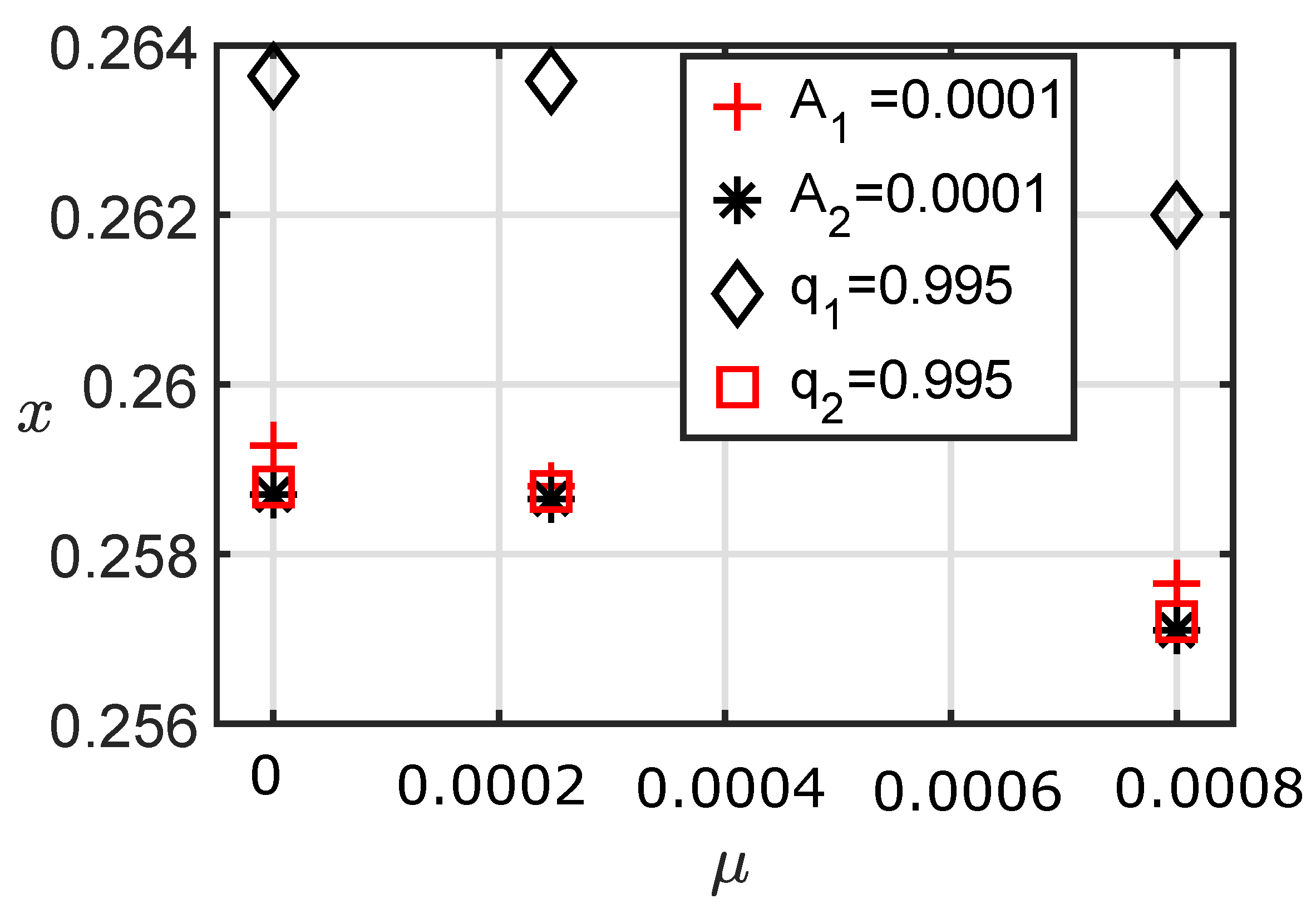
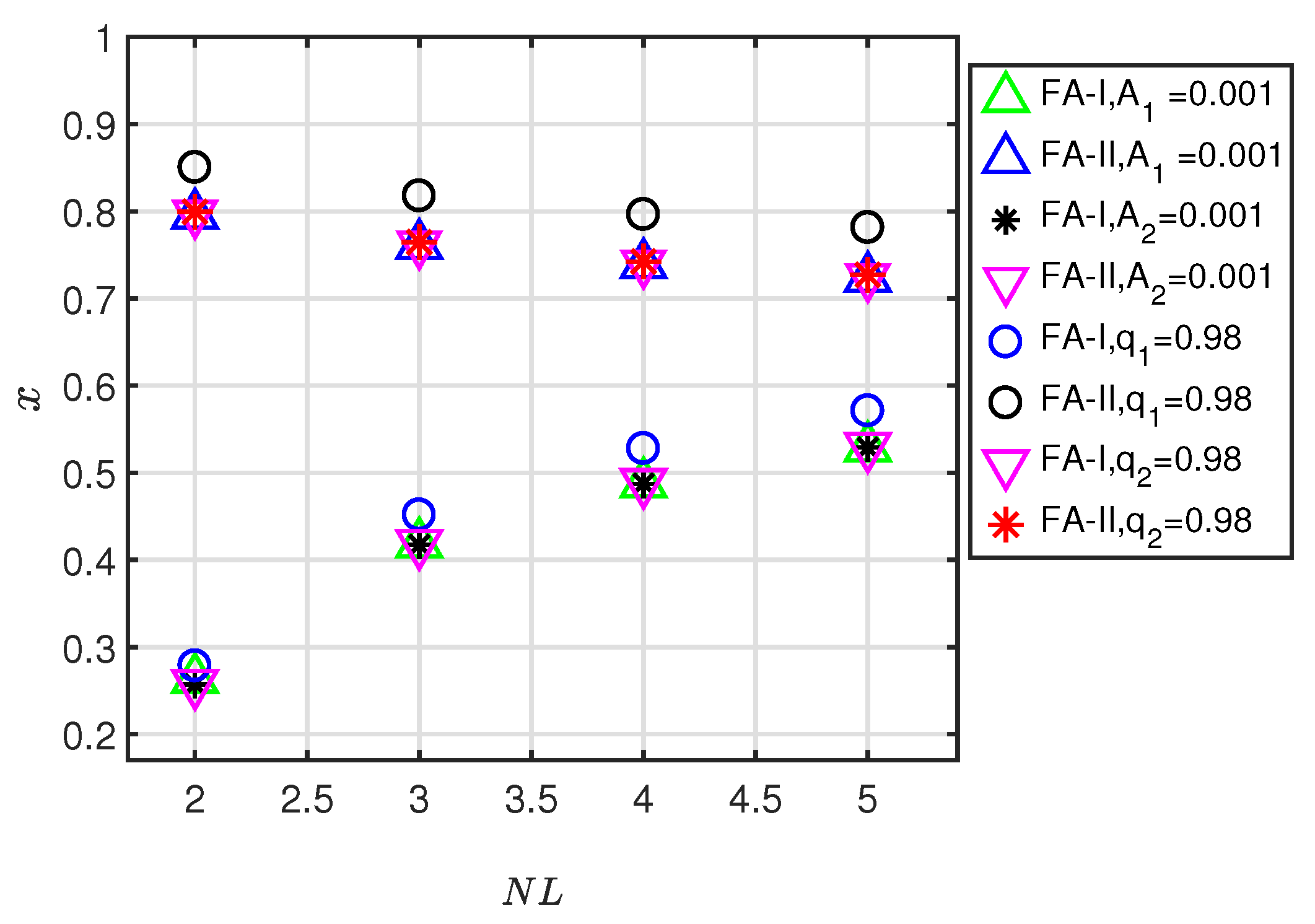
7.1. Initial Position Analysis of Periodic Orbits
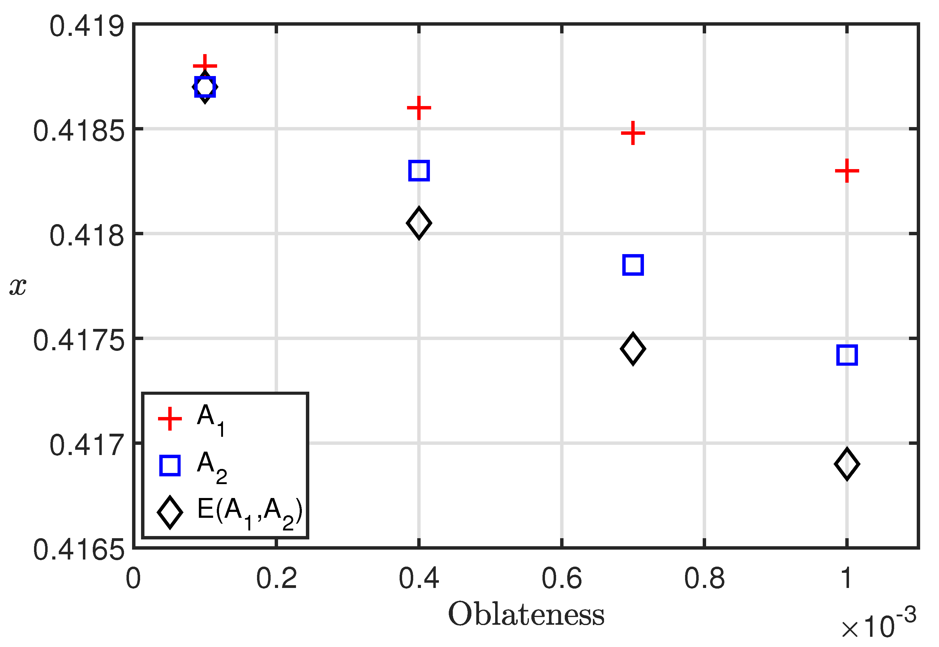
- Effect of is the largest among all the perturbations which shifts x towards the one (i.e., near to the less massive primary).
- Under the combine effects of and , x shifts towards the one.
- The next higher effect on x is due to .
- and both shift the x towards the zero (i.e., near to the more massive primary).
- Under the effects of and , x shifts towards the zero.
- has less effect than in shifting x towards zero.
- As a result, combine effects of is more compare to in shifting x towards one.
- combine effects of shift x more towards zero compared to .
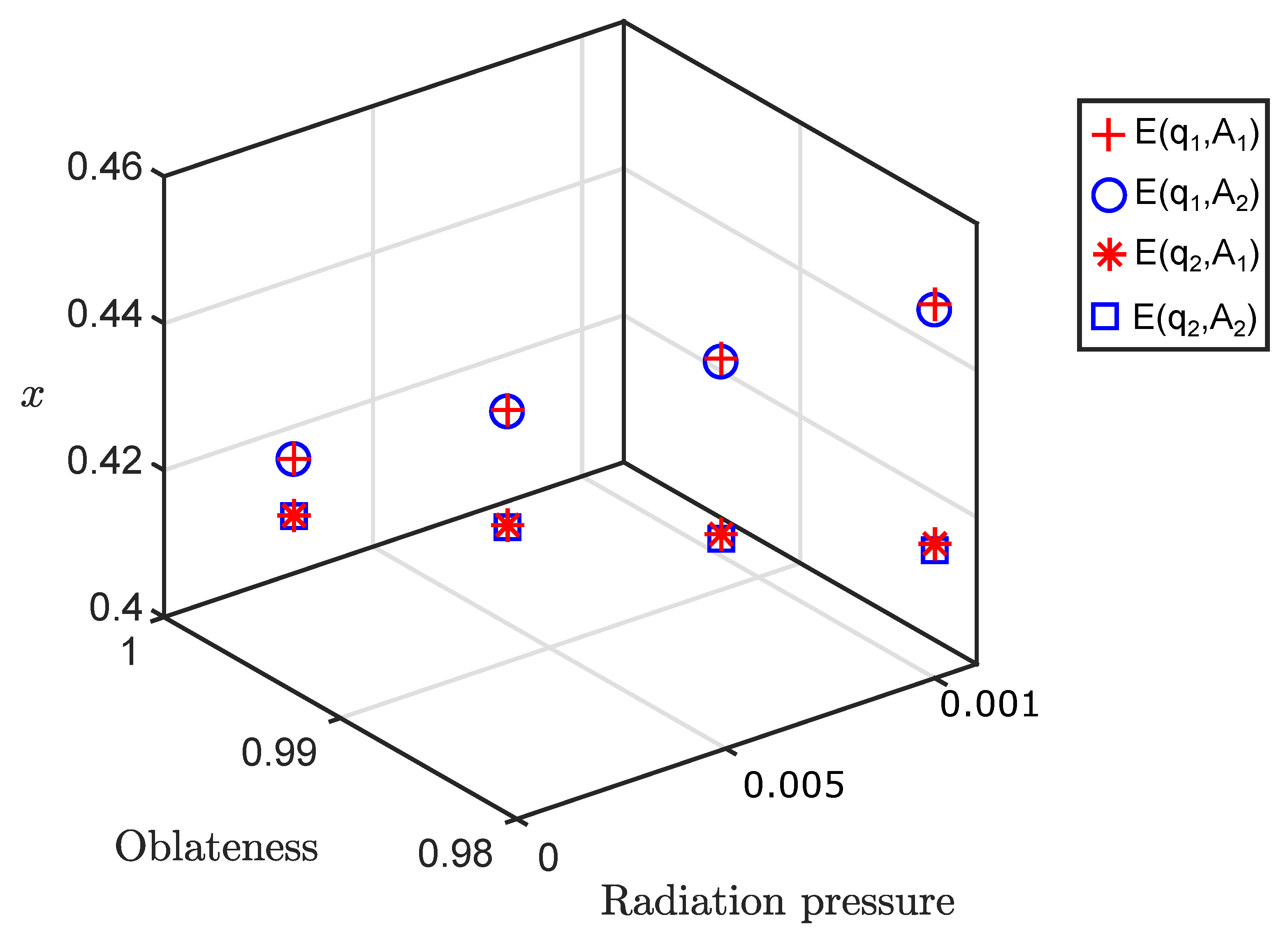
- Effect of on x of periodic orbits from both families is significant compared to other perturbations.
- Under the combine effects of the perturbations in which is one of the perturbation parameter (i.e., , and ) initial position x of the periodic orbits shifts towards the one.
- Also, the second largest effect on x shift towards zero is due to .
- As a result, initial position x of both family orbits shifts towards the zero as perturbations rises except in the case of 2:1 orbit.
- From the second and seventeenth rows of Table 4, it can be observed that only for 2:1 resonant orbit initial position x shifts towards 1 due to increment in the perturbation .
- Effect of is much more less than effect of in shifting x towards zero.
- As a result, combine d effect of is more in shifting x towards one in comparison to and .
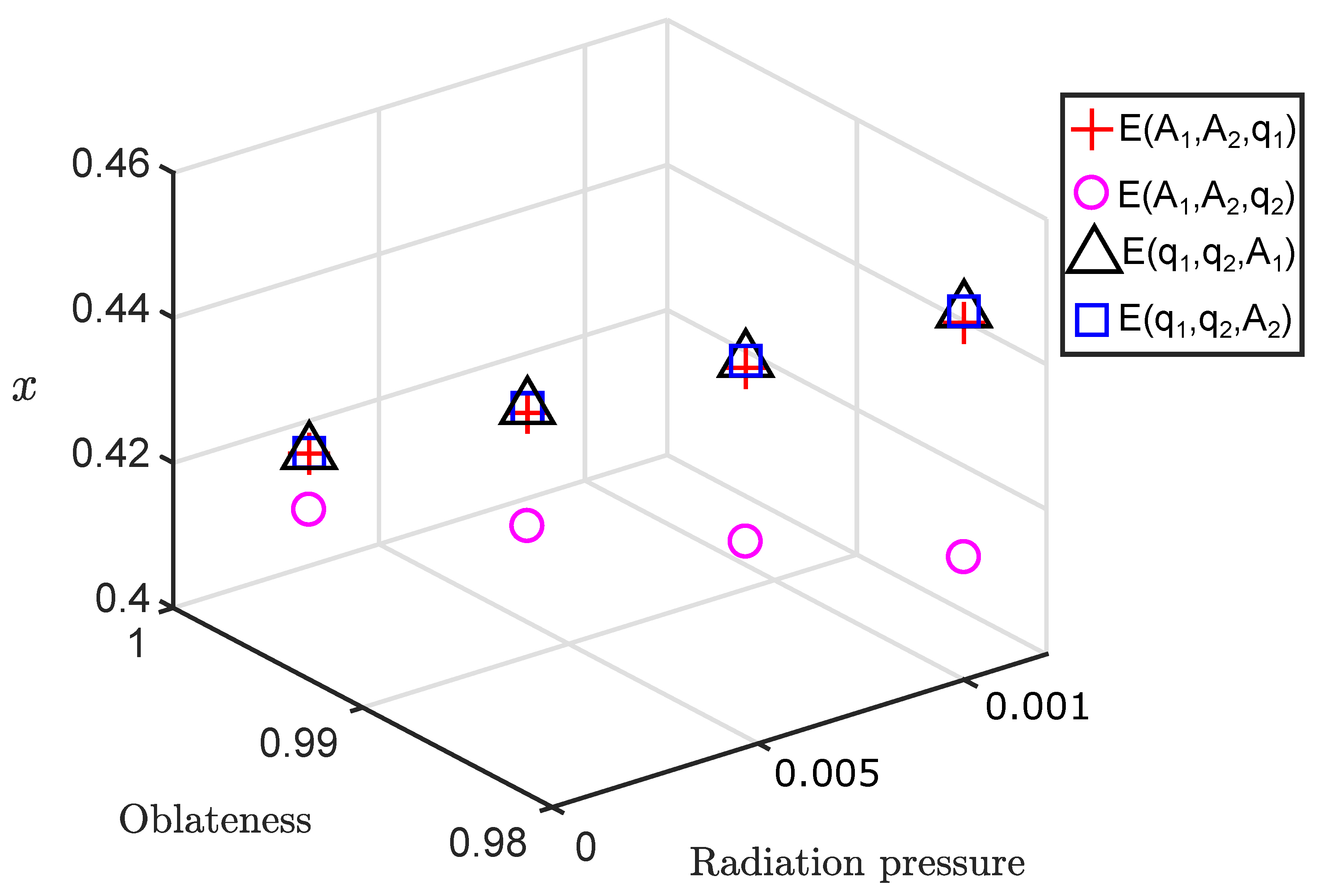
- Effect of is more than effect of on x.
- Increment in shifts x towards zero where as increment in shifts x towards one.
- As a result, combine effect of is more than in shifting x towards one.
- For both families of periodic orbits, under the combine increment of four perturbations , x shifts towards the one observed in Table 4.
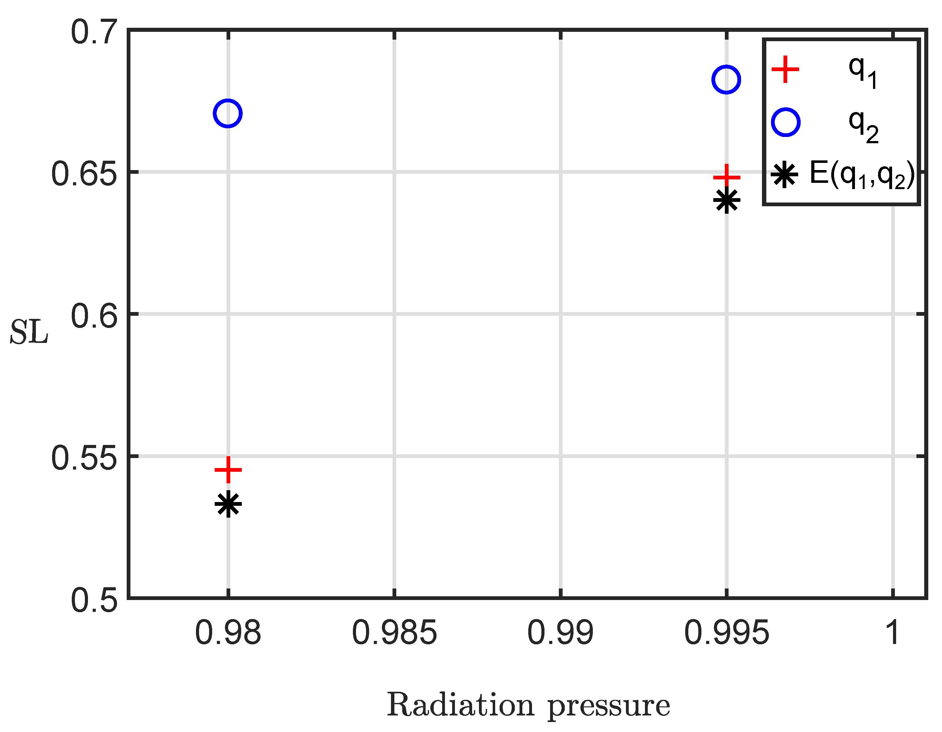
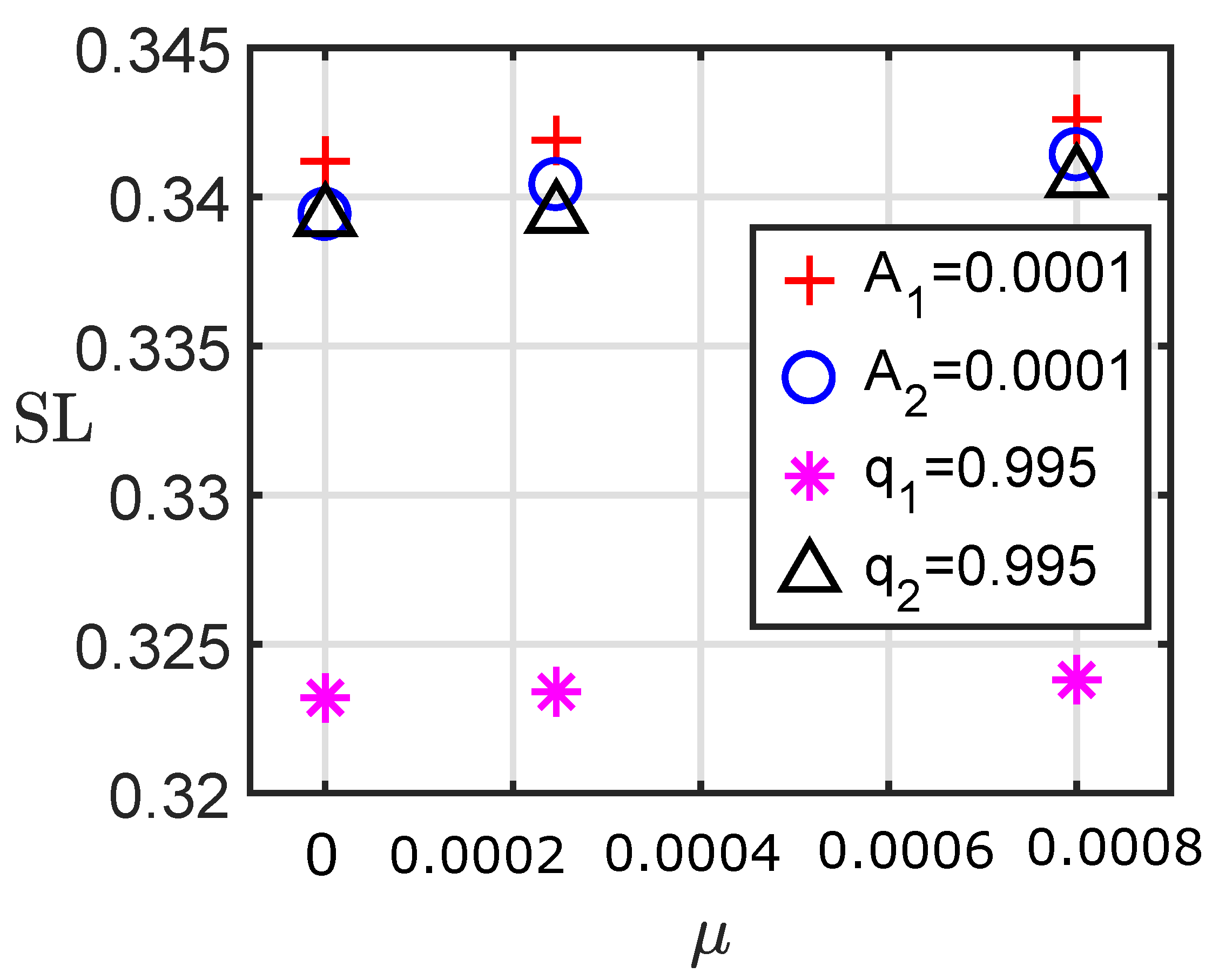
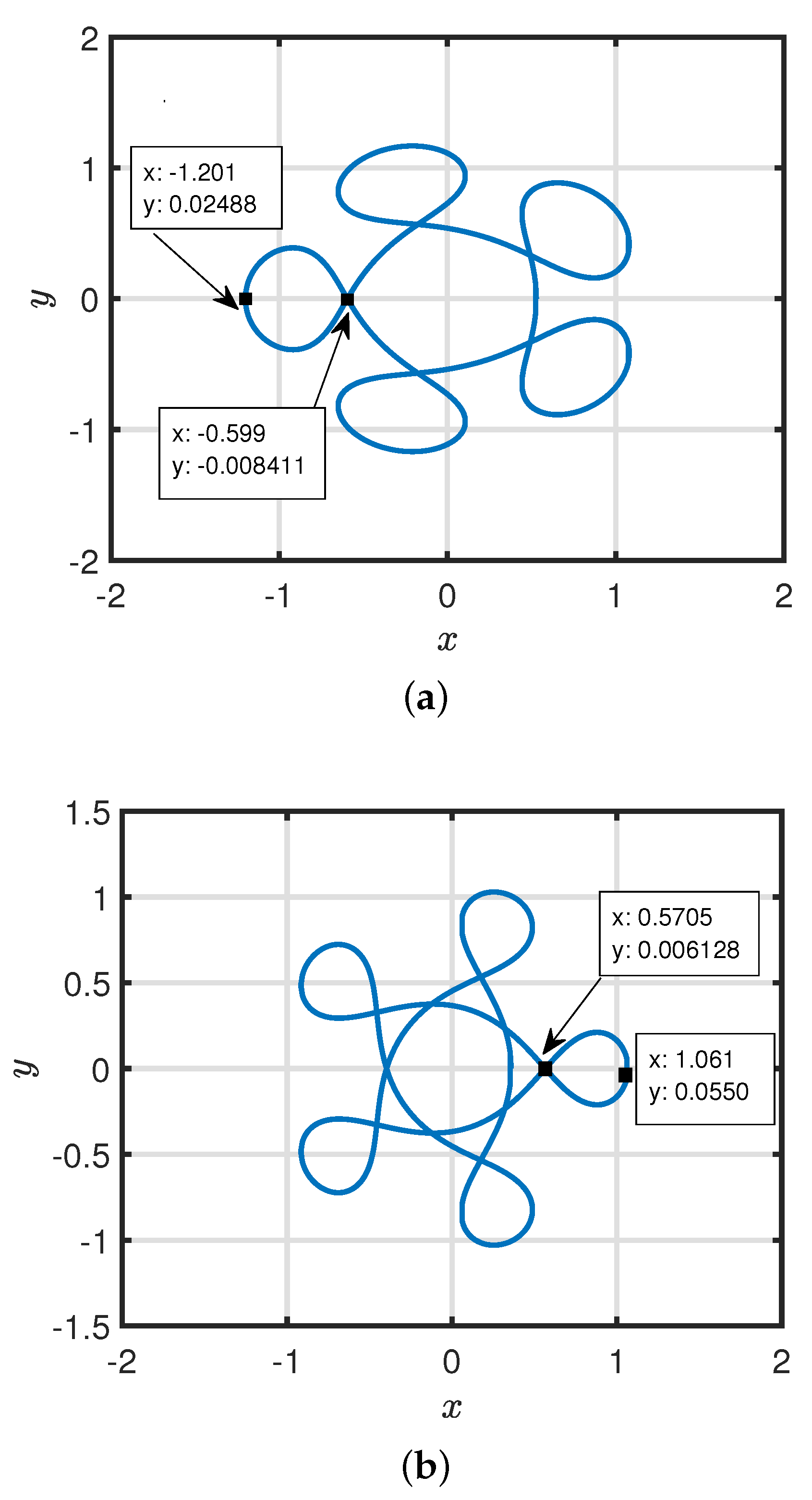
7.2. Size Loops Analysis of Periodic Orbits
8. Physical and Geometrical Parameters Analysis of Periodic Orbits
9. Conclusions
- Effect of perturbations on initial position () of periodic orbits.
- Effect of perturbations on size of the loop () of periodic orbits.
- Effect of Jacobi constant on and of perturbed periodic orbits.
- Effect of mass factor on and of perturbed periodic orbits.
- Effect of resonance order on and of perturbed periodic orbits.
- Effect of number of loops on and of perturbed periodic orbits.
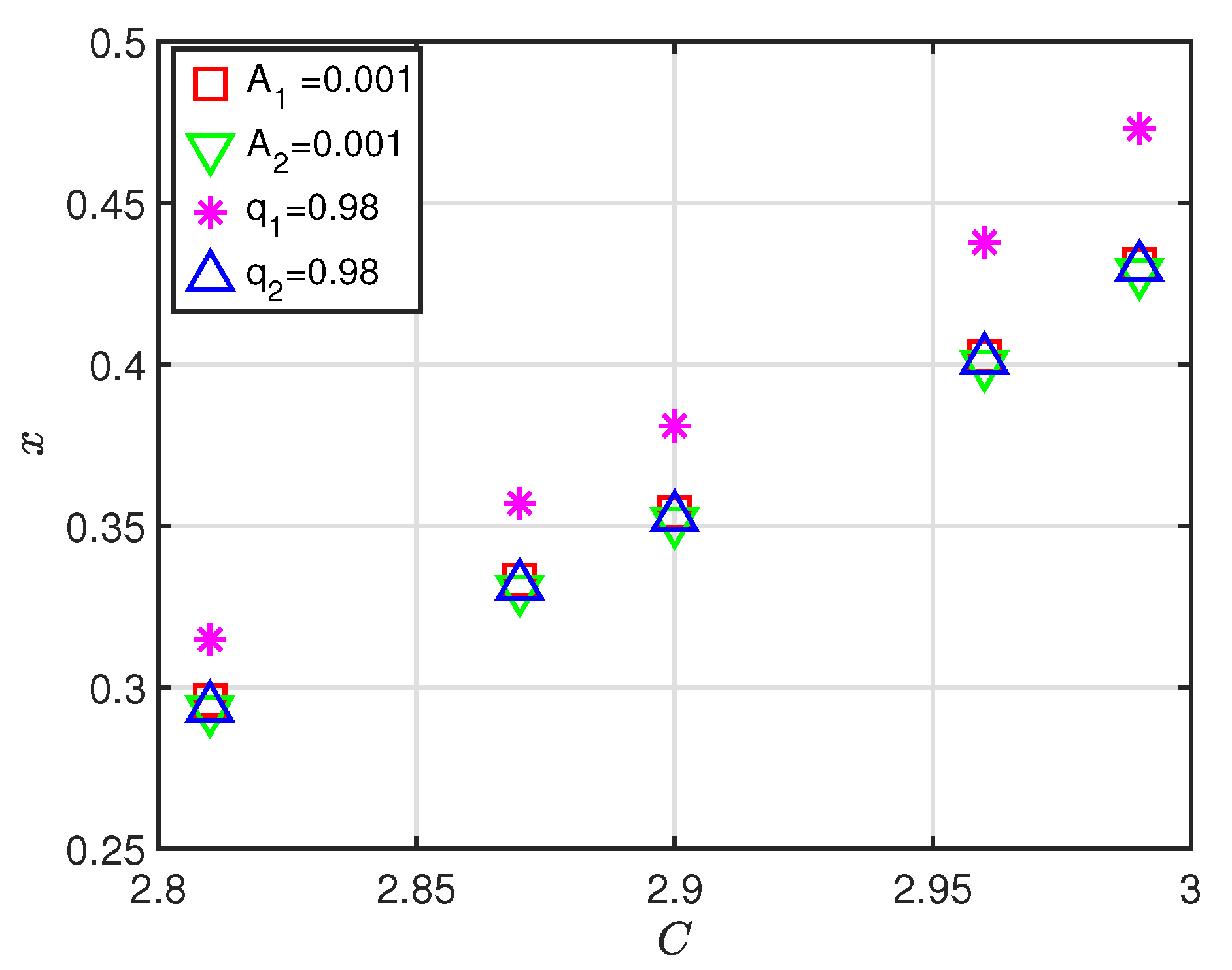
- Degree of perturbations effects from highest to smallest on the initial position of periodic orbits are radiation pressure of bigger primary, oblateness coefficient of smaller primary, oblateness coefficient of bigger primary and radiation pressure of the smaller primary
- Radiation pressure shifts initial condition towards smaller primary. Whereas, oblateness coefficient shifts initial condition towards bigger primary.
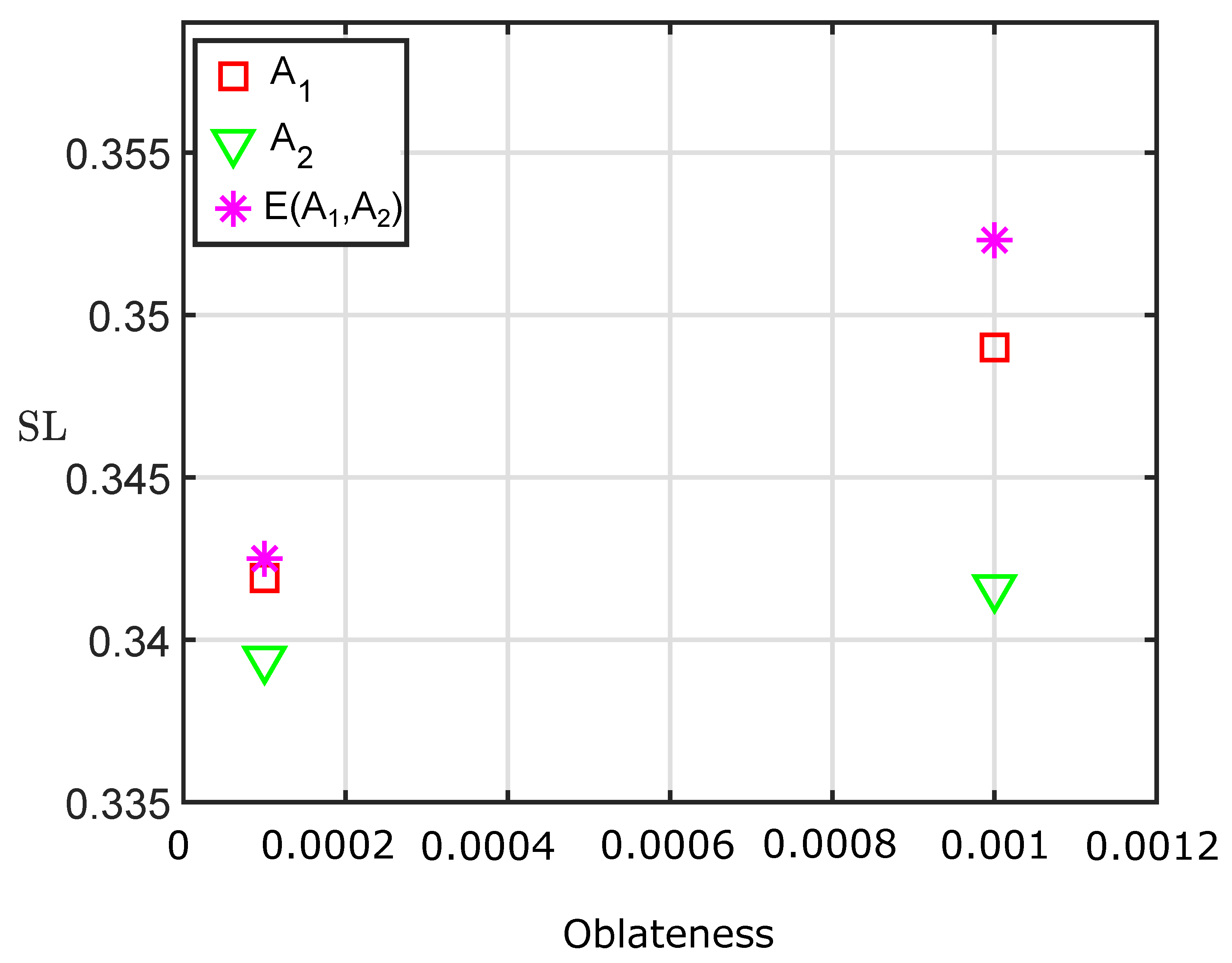
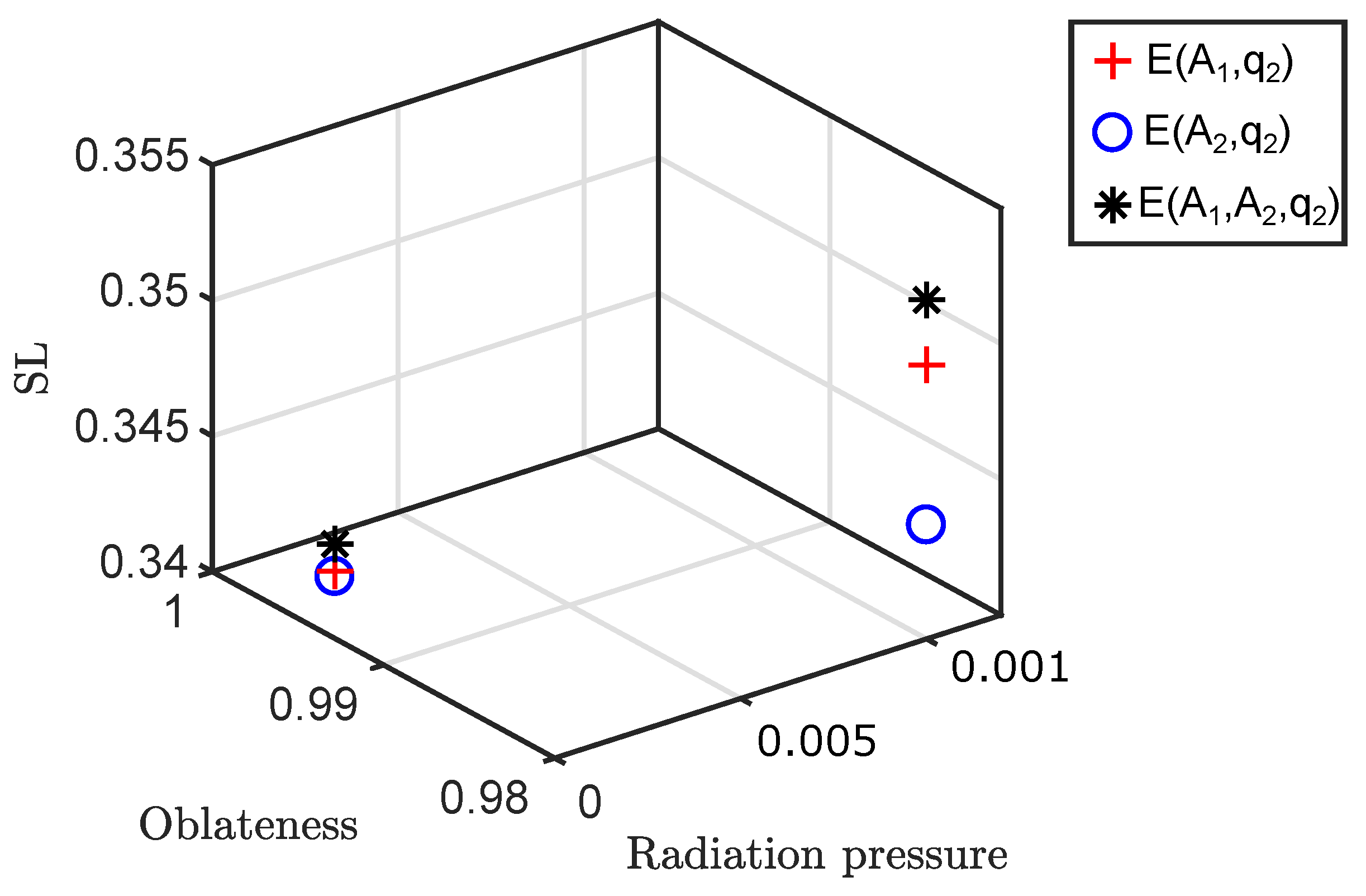
- Size of the loops is highest affected by radiation pressure of bigger primary, followed by oblateness coefficient of bigger primary, followed by oblateness coefficient of smaller primary and then lastly by radiation pressure of the smaller primary.
- Radiation pressure reduces the size of the loops. Whereas, oblateness coefficient increases the size of the loops.
- Increment in Jacobi constance shifts initial position towards smaller primary and reduces the size of the loops.
- Increment in the mass factor shifts initial position towards bigger primary and increases the size of the loops.
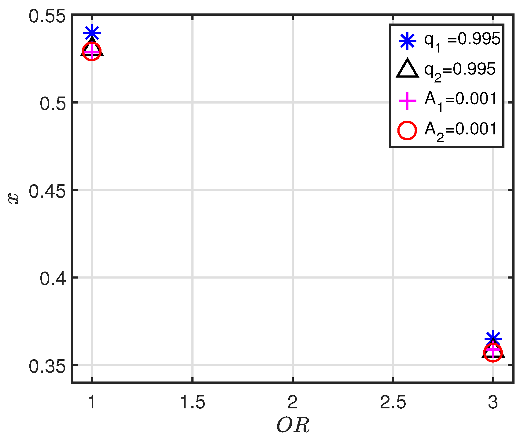
- Increment in the order of resonance shifts initial position towards bigger primary and reduces the size of the loops.
- Increment in the number of loops shifts initial position of family–I periodic orbits towards smaller primary.
- Increment in the number of loops shifts initial position of family– periodic orbits towards bigger primary.
Author Contributions
Funding
Data Availability Statement
Acknowledgments
Conflicts of Interest
Abbreviations
| RTBP | Restricted three-body problem |
| CRTBP | Circular restricted three-body problem |
| PSS | Poincaré surface section |
| Combine effects of and | |
| Combine effects of and | |
| Combine effects of and | |
| Combine effects of and |
| Combine effects of and | |
| Combine effects of and | |
| Combine effects of , and | |
| Combine effects of , and | |
| Combine effects of , and | |
| Combine effects of , and | |
| Combine effects of , , and |
References
- Szebehely, V.; Grebenikov, E. Theory of Orbits-The Restricted Problem of Three Bodies. Sov. Astron. 1969, 13, 364. [Google Scholar]
- Murray, C.D.; Dermott, S.F. Solar System Dynamics; Cambridge University Press: Cambridge, UK, 1999. [Google Scholar]
- Duffy, B. Analytical Methods and Perturbation Theory for the Elliptic Restricted three-body Problem of Astrodynamics. Ph.D. Thesis, The George Washington University, Washington, DC, USA, 2012. [Google Scholar]
- Melton, R.G. Fundamentals of astrodynamics and applications. J. Guid. Control. Dyn. 1998, 21, 672. [Google Scholar] [CrossRef]
- Sharma, R.K.; Taqvi, Z.; Bhatnagar, K. Existence and stability of libration points in the restricted three-body problem when the primaries are triaxial rigid bodies. Celest. Mech. Dyn. Astron. 2001, 79, 119–133. [Google Scholar] [CrossRef]
- Singh, J. Combined effects of perturbations, radiation, and oblateness on the nonlinear stability of triangular points in the restricted three-body problem. Astrophys. Space Sci. 2011, 332, 331–339. [Google Scholar] [CrossRef]
- Selim, H.H.; Guirao, J.L.; Abouelmagd, E.I. Libration points in the restricted three-body problem: Euler angles, existence and stability. Discret. Contin. Dyn. Syst.-S 2018, 12, 703. [Google Scholar] [CrossRef]
- Hallan, P.; Rana, N. Effect of perturbations in coriolis and centrifugal forces on the location and stability of the equilibrium point in the Robe’s circular restricted three body problem. Planet. Space Sci. 2001, 49, 957–960. [Google Scholar] [CrossRef]
- Kalantonis, V.; Douskos, C.; Perdios, E. Numerical determination of homoclinic and heteroclinic orbits at collinear equilibria in the restricted three-body problem with oblateness. Celest. Mech. Dyn. Astron. 2006, 94, 135–153. [Google Scholar] [CrossRef]
- Singh, J.; Kalantonis, V.; Gyegwe, J.M.; Perdiou, A. Periodic motions around the collinear equilibrium points of the R3BP where the primary is a triaxial rigid body and the secondary is an oblate spheroid. Astrophys. J. Suppl. Ser. 2016, 227, 13. [Google Scholar] [CrossRef]
- Yousuf, S.; Kishor, R. Effects of the albedo and disc on the zero velocity curves and linear stability of equilibrium points in the generalized restricted three-body problem. Mon. Not. R. Astron. Soc. 2019, 488, 1894–1907. [Google Scholar] [CrossRef]
- Kalantonis, V.S.; Perdiou, A.E.; Perdios, E.A. On the stability of the triangular equilibrium points in the elliptic restricted three-body problem with radiation and oblateness. Math. Anal. Appl. 2019, 154, 273–286. [Google Scholar]
- Gao, F.; Wang, Y. Approximate analytical periodic solutions to the restricted three-body problem with perturbation, oblateness, radiation and varying mass. Universe 2020, 6, 110. [Google Scholar] [CrossRef]
- Gao, F.; Wang, R. Bifurcation analysis and periodic solutions of the HD 191408 system with triaxial and radiative perturbations. Universe 2020, 6, 35. [Google Scholar] [CrossRef]
- Abouelmagd, E.I. The effect of photogravitational force and oblateness in the perturbed restricted three-body problem. Astrophys. Space Sci. 2013, 346, 51–69. [Google Scholar] [CrossRef]
- Patel, B.M.; Pathak, N.M.; Abouelmagd, E.I. First-order resonant in periodic orbits. Int. J. Geom. Methods Mod. Phys. 2021, 18, 2150011. [Google Scholar] [CrossRef]
- Patel, B.M.; Pathak, N.M.; Abouelmagd, E.I. Stability analysis of first order resonant periodic orbit. Icarus 2022, 387, 115165. [Google Scholar] [CrossRef]
- Érdi, B.; Rajnai, R.; Sándor, Z.; Forgács-Dajka, E. Stability of higher order resonances in the restricted three-body problem. Celest. Mech. Dyn. Astron. 2012, 113, 95–112. [Google Scholar] [CrossRef]
- Luk’yanov, L. On the restricted circular conservative three-body problem with variable masses. Astron. Lett. 2009, 35, 349–359. [Google Scholar] [CrossRef]
- Pal, A.K.; Abouelmagd, E.I.; Kishor, R. Effect of Moon perturbation on the energy curves and equilibrium points in the Sun–Earth–Moon system. New Astron. 2021, 84, 101505. [Google Scholar] [CrossRef]
- Bairwa, L.K.; Pal, A.K.; Kumari, R.; Alhowaity, S.; Abouelmagd, E.I. Study of Lagrange Points in the Earth–Moon System with Continuation Fractional Potential. Fractal Fract. 2022, 6, 321. [Google Scholar] [CrossRef]
- Suleiman, R.; Umar, A.; Singh, J. Collinear Points in the Photogravitational ER3BP with Zonal Harmonics of the Secondary. Differ. Equ. Dyn. Syst. 2020, 28, 901–922. [Google Scholar] [CrossRef]
- Sheth, D.; Thomas, V. Halo orbits around L1, L2, and L3 in the photogravitational Sun–Mars elliptical restricted three-body problem. Astrophys. Space Sci. 2022, 367, 99. [Google Scholar] [CrossRef]
- Howell, K.C.; Spencer, D.B. Periodic orbits in the restricted four-body problem. Acta Astronaut. 1986, 13, 473–479. [Google Scholar] [CrossRef]
- Liu, C.; Gong, S. Hill stability of the satellite in the elliptic restricted four-body problem. Astrophys. Space Sci. 2018, 363, 162. [Google Scholar] [CrossRef]
- Carletta, S.; Pontani, M.; Teofilatto, P. Characterization of Low-Energy Quasiperiodic Orbits in the Elliptic Restricted 4-Body Problem with Orbital Resonance. Aerospace 2022, 9, 175. [Google Scholar] [CrossRef]
- Pathak, N.; Thomas, V.; Abouelmagd, E.I. The perturbed photogravitational restricted three-body problem: Analysis of resonant periodic orbits. Discret. Contin. Dyn. Syst.-S 2019, 12, 849. [Google Scholar] [CrossRef]
- Pathak, N.; Abouelmagd, E.I.; Thomas, V. On Higher Order Resonant Periodic Orbits in the Photo–Gravitational Planar Restricted three-body Problem with Oblateness. J. Astronaut. Sci. 2019, 66, 475–505. [Google Scholar] [CrossRef]
- Patel, B.M.; Pathak, N.M.; Abouelmagd, E.I. Nonlinear regression multivariate model for first order resonant periodic orbits and error analysis. Planet. Space Sci. 2022, 219, 105516. [Google Scholar] [CrossRef]
- Ugai, S.; Ichikawa, A. Lunar Synchronous Orbits in the Earth-Moon Circular-Restricted Three-Body Problem. J. Guid. Control. Dyn. 2010, 33, 995–1000. [Google Scholar] [CrossRef]
- Musielak, Z.E.; Quarles, B. The three-body problem. Rep. Prog. Phys. 2014, 77, 065901. [Google Scholar] [CrossRef]
- Heinrich, W.; Roesler, S.; Schraube, H. Physics of cosmic radiation fields. Radiat. Prot. Dosim. 1999, 86, 253–258. [Google Scholar] [CrossRef]
- Schuerman, D.W. The restricted three-body problem including radiation pressure. Astrophys. J. 1980, 238, 337–342. [Google Scholar] [CrossRef]
- Zotos, E.E. Fractal basins of attraction in the planar circular restricted three-body problem with oblateness and radiation pressure. Astrophys. Space Sci. 2016, 361, 181. [Google Scholar] [CrossRef]
- Dutt, P.; Sharma, R. Evolution of periodic orbits in the Sun-Mars system. J. Guid. Control. Dyn. 2011, 34, 635–644. [Google Scholar] [CrossRef]
- Poynting, J. Radiation in the solar system: Its effect on temperature and its pressure on small bodies. Mon. Not. R. Astron. Soc. 1903, 64, 1. [Google Scholar] [CrossRef]
- Radzievskii, V. The restricted problem of three bodies taking account of light pressure. Astron. Zhurnal 1950, 27, 250. [Google Scholar]
- Chernikov, Y.A. The Photogravitational Restricted Three-Body Problem. Sov. Astron. 1970, 14, 176. [Google Scholar]
- Kunitsyn, A.; Perezhogin, A. On the stability of triangular libration points of the photogravitational restricted circular three-body problem. Celest. Mech. 1978, 18, 395–408. [Google Scholar] [CrossRef]
- Schuerman, D.W. The effect of radiation pressure on the restricted three-body problem. In Symposium-International Astronomical Union; Cambridge University Press: Cambridge, UK, 1980; Volume 90, pp. 285–288. [Google Scholar]
- Markellos, V.; Perdios, E.; Papadakis, K. The stability of inner collinear equilibrium points in the photogravitational elliptic restricted problem. Astrophys. Space Sci. 1993, 199, 139–146. [Google Scholar] [CrossRef]
- Papadakis, K. Asymptotic orbits at the triangular equilibria in the photogravitational restricted three-body problem. Astrophys. Space Sci. 2006, 305, 57–66. [Google Scholar] [CrossRef]
- AbdulRaheem, A.; Singh, J. Combined effects of perturbations, radiation, and oblateness on the stability of equilibrium points in the restricted three-body problem. Astron. J. 2006, 131, 1880. [Google Scholar] [CrossRef]
- Vishnu Namboodiri, N.; Sudheer Reddy, D.; Sharma, R.K. Effect of oblateness and radiation pressure on angular frequencies at collinear points. Astrophys. Space Sci. 2008, 318, 161–168. [Google Scholar] [CrossRef]
- Proctor, R.A. Essays on Astronomy: A Series of Papers on Planets and Meteors, the Sun and Sun-Surrounding Space, Stars and Star Cloudlets; and a Dissertation on the Approaching Transits of Venus. Preceded by a Sketch of the Life and Works of Sir John Herschel; Longman’s, Green, and Company. 1872. [Google Scholar]
- Kaufmann, W.J., III. Universe, 2nd ed.; W H Freeman and Co.: USA, 1988. [Google Scholar]
- Ershkov, S.V. About tidal evolution of quasi-periodic orbits of satellites. Earth Moon Planets 2017, 120, 15–30. [Google Scholar] [CrossRef]
- Ershkov, S.; Leshchenko, D.; Abouelmagd, E.I. About influence of differential rotation in convection zone of gaseous or fluid giant planet (Uranus) onto the parameters of orbits of satellites. Eur. Phys. J. Plus 2021, 136, 1–9. [Google Scholar] [CrossRef]
- Kalvouridis, T.; Arribas, M.; Elipe, A. Parametric evolution of periodic orbits in the restricted four-body problem with radiation pressure. Planet. Space Sci. 2007, 55, 475–493. [Google Scholar] [CrossRef]
- Lukyanov, L. Family of Libration Points in the Restricted Photogravitational Three-Body Problem. Sov. Astron. 1988, 32, 215. [Google Scholar]
- Ansari, A.A.; Abouelmagd, E.I. Gravitational potential formulae between two bodies with finite dimensions. Astron. Nachrichten 2020, 341, 656–668. [Google Scholar] [CrossRef]
- McCuskey, S.W. Introduction to Celestial Mechanics; Addison-Wesley Publishinig Company: Reading, MA, USA, 1963. [Google Scholar]


| 0.0000 | 0.0000 | 1.000 | 1.000 | 0.95693741 | 1.04382876 | −1.00010255 |
| 0.0001 | 0.0000 | 1.000 | 1.000 | 0.95694108 | 1.04382519 | −1.00010257 |
| 0.0000 | 0.0000 | 0.995 | 1.000 | 0.95635803 | 1.04329584 | −0.99843327 |
| 0.0001 | 0.0000 | 0.995 | 1.000 | 0.95636177 | 1.04329232 | −0.99843345 |
| 0.0001 | 0.0001 | 1.000 | 0.995 | 0.95592836 | 1.04480535 | −1.00005248 |
| 0.0001 | 0.0001 | 0.995 | 1.000 | 0.95530538 | 1.04437017 | −0.99838355 |
| 0.0000 | 0.0001 | 0.995 | 0.995 | 0.95537066 | 1.04430062 | −0.99838326 |
| 0.0001 | 0.0001 | 0.995 | 0.995 | 0.95537431 | 1.04429719 | −0.99838345 |
| 0.001 | 0.000 | 1.000 | 1.000 | 0.95697410 | 1.04379311 | −1.00010267 |
| 0.000 | 0.000 | 0.980 | 1.000 | 0.95451793 | 1.04176914 | −0.99339163 |
| 0.001 | 0.000 | 0.980 | 1.000 | 0.95455716 | 1.04173546 | −0.99339846 |
| 0.000 | 0.001 | 0.980 | 0.980 | 0.94797343 | 1.04902983 | −0.99289510 |
| 0.001 | 0.001 | 0.980 | 1.000 | 0.94774406 | 1.04927703 | −0.99290358 |
| 0.000 | 0.001 | 0.980 | 0.980 | 0.94797343 | 1.04902983 | −0.99289510 |
| 0.001 | 0.001 | 0.980 | 0.980 | 0.94801050 | 1.04899904 | −0.99290317 |
| Family–I | Family–II | |||||||||||
|---|---|---|---|---|---|---|---|---|---|---|---|---|
| 2 | 2:1 | 0.0001 | 0 | 1 | 1 | 0.25880 | 2:3 | 0.0001 | 0 | 1 | 1 | 0.79910 |
| 0 | 0.0001 | 1 | 1 | 0.25820 | 0 | 0.0001 | 1 | 1 | 0.79925 | |||
| 0 | 0 | 0.995 | 1 | 0.26314 | 0 | 0 | 0.995 | 1 | 0.81140 | |||
| 0 | 0 | 0 | 0.995 | 0.25830 | 0 | 0 | 0 | 0.995 | 0.79948 | |||
| 3 | 3:2 | 0.0001 | 0 | 1 | 1 | 0.41880 | 3:4 | 0.0001 | 0 | 1 | 1 | 0.76420 |
| 0 | 0.0001 | 1 | 1 | 0.41870 | 0 | 0.0001 | 1 | 1 | 0.76440 | |||
| 0 | 0 | 0.995 | 1 | 0.42655 | 0 | 0 | 0.995 | 1 | 0.77690 | |||
| 0 | 0 | 0 | 0.995 | 0.41890 | 0 | 0 | 0 | 0.995 | 0.76460 | |||
| 4 | 4:3 | 0.0001 | 0 | 1 | 1 | 0.48880 | 4:5 | 0.0001 | 0 | 1 | 1 | 0.74200 |
| 0 | 0.0001 | 1 | 1 | 0.48816 | 0 | 0.0001 | 1 | 1 | 0.74220 | |||
| 0 | 0 | 0.995 | 1 | 0.49745 | 0 | 0 | 0.995 | 1 | 0.75490 | |||
| 0 | 0 | 0 | 0.995 | 0.48830 | 0 | 0 | 0 | 0.995 | 0.74245 | |||
| 5 | 5:4 | 0.0001 | 0 | 1 | 1 | 0.53030 | 5:6 | 0.0001 | 0 | 1 | 1 | 0.72670 |
| 0 | 0.0001 | 1 | 1 | 0.53030 | 0 | 0.0001 | 1 | 1 | 0.72680 | |||
| 0 | 0 | 0.995 | 1 | 0.53970 | 0 | 0 | 0.995 | 1 | 0.73960 | |||
| 0 | 0 | 0 | 0.995 | 0.53040 | 0 | 0 | 0 | 0.995 | 0.72710 | |||
| 2 | 2:1 | 0.001 | 0 | 1 | 1 | 0.26298 | 2:3 | 0.001 | 0 | 1 | 1 | 0.79575 |
| 0 | 0.001 | 1 | 1 | 0.25739 | 0 | 0.001 | 1 | 1 | 0.79720 | |||
| 0 | 0 | 0.98 | 1 | 0.27855 | 0 | 0 | 0.98 | 1 | 0.85040 | |||
| 0 | 0 | 0 | 0.98 | 0.25830 | 0 | 0 | 0 | 0.98 | 0.79950 | |||
| 3 | 3:2 | 0.001 | 0 | 1 | 1 | 0.41830 | 3:4 | 0.001 | 0 | 1 | 1 | 0.76080 |
| 0 | 0.001 | 1 | 1 | 0.41742 | 0 | 0.001 | 1 | 1 | 0.76225 | |||
| 0 | 0 | 0.98 | 1 | 0.45170 | 0 | 0 | 0.98 | 1 | 0.81775 | |||
| 0 | 0 | 0 | 0.98 | 0.41882 | 0 | 0 | 0 | 0.98 | 0.76460 | |||
| 4 | 4:3 | 0.001 | 0 | 1 | 1 | 0.48725 | 4:5 | 0.001 | 0 | 1 | 1 | 0.73860 |
| 0 | 0.001 | 1 | 1 | 0.48730 | 0 | 0.001 | 1 | 1 | 0.74010 | |||
| 0 | 0 | 0.98 | 1 | 0.52790 | 0 | 0 | 0.98 | 1 | 0.79640 | |||
| 0 | 0 | 0 | 0.98 | 0.48890 | 0 | 0 | 0 | 0.98 | 0.74242 | |||
| 5 | 5:4 | 0.001 | 0 | 1 | 1 | 0.52860 | 5:6 | 0.001 | 0 | 1 | 1 | 0.72330 |
| 0 | 0.001 | 1 | 1 | 0.52890 | 0 | 0.001 | 1 | 1 | 0.72470 | |||
| 0 | 0 | 0.98 | 1 | 0.57110 | 0 | 0 | 0.98 | 1 | 0.78140 | |||
| 0 | 0 | 0 | 0.98 | 0.53030 | 0 | 0 | 0 | 0.98 | 0.72710 | |||
| Family–I | Family–II | |||||||||||
|---|---|---|---|---|---|---|---|---|---|---|---|---|
| 2 | 2:1 | 0.0001 | 0.0001 | 1 | 1 | 0.25870 | 2:3 | 0.0001 | 0.0001 | 1 | 1 | 0.79890 |
| 0.0001 | 0 | 0.995 | 1 | 0.26362 | 0.0001 | 0 | 0.995 | 1 | 0.81100 | |||
| 0.0001 | 0 | 1 | 0.995 | 0.25880 | 0.0001 | 0 | 1 | 0.995 | 0.79910 | |||
| 0 | 0.0001 | 0.995 | 1 | 0.26305 | 0 | 0.0001 | 0.995 | 1 | 0.81120 | |||
| 0 | 0.0001 | 1 | 0.995 | 0.25820 | 0 | 0.0001 | 1 | 0.995 | 0.79925 | |||
| 0 | 0 | 0.995 | 0.995 | 0.26315 | 0 | 0 | 0.995 | 0.995 | 0.81140 | |||
| 3 | 3:2 | 0.0001 | 0.0001 | 1 | 1 | 0.41870 | 3:4 | 0.0001 | 0.0001 | 1 | 1 | 0.76400 |
| 0.0001 | 0 | 0.995 | 1 | 0.42650 | 0.0001 | 0 | 0.995 | 1 | 0.77651 | |||
| 0.0001 | 0 | 1 | 0.995 | 0.41880 | 0.0001 | 0 | 1 | 0.995 | 0.76420 | |||
| 0 | 0.0001 | 0.995 | 1 | 0.42640 | 0 | 0.0001 | 0.995 | 1 | 0.77670 | |||
| 0 | 0.0001 | 1 | 0.995 | 0.41870 | 0 | 0.0001 | 1 | 0.995 | 0.76440 | |||
| 0 | 0 | 0.995 | 0.995 | 0.42660 | 0 | 0 | 0.995 | 0.995 | 0.77690 | |||
| 4 | 4:3 | 0.0001 | 0.0001 | 1 | 1 | 0.48860 | 4:5 | 0.0001 | 0.0001 | 1 | 1 | 0.74180 |
| 0.0001 | 0 | 0.995 | 1 | 0.49785 | 0.0001 | 0 | 0.995 | 1 | 0.75450 | |||
| 0.0001 | 0 | 1 | 0.995 | 0.48875 | 0.0001 | 0 | 1 | 0.995 | 0.74210 | |||
| 0 | 0.0001 | 0.995 | 1 | 0.49780 | 0 | 0.0001 | 0.995 | 1 | 0.75470 | |||
| 0 | 0.0001 | 1 | 0.995 | 0.48880 | 0 | 0.0001 | 1 | 0.995 | 0.74220 | |||
| 0 | 0 | 0.995 | 0.995 | 0.49800 | 0 | 0 | 0.995 | 0.995 | 0.75490 | |||
| 2 | 2:1 | 0.001 | 0.001 | 1 | 1 | 0.26210 | 2:3 | 0.001 | 0.001 | 1 | 1 | 0.79350 |
| 0.001 | 0 | 0.98 | 1 | 0.28289 | 0.001 | 0 | 0.98 | 1 | 0.84620 | |||
| 0.001 | 0 | 1 | 0.98 | 0.26298 | 0.001 | 0 | 1 | 0.98 | 0.79570 | |||
| 0 | 0.001 | 0.98 | 1 | 0.27755 | 0 | 0.001 | 0.98 | 1 | 0.84780 | |||
| 0 | 0.001 | 1 | 0.98 | 0.25740 | 0 | 0.001 | 1 | 0.98 | 0.79715 | |||
| 0 | 0 | 0.98 | 0.98 | 0.27855 | 0 | 0 | 0.98 | 0.98 | 0.85035 | |||
| 3 | 3:2 | 0.001 | 0.001 | 1 | 1 | 0.41690 | 3:4 | 0.001 | 0.001 | 1 | 1 | 0.75850 |
| 0.001 | 0 | 0.98 | 1 | 0.45090 | 0.001 | 0 | 0.98 | 1 | 0.81340 | |||
| 0.001 | 0 | 1 | 0.98 | 0.41822 | 0.001 | 0 | 1 | 0.98 | 0.76080 | |||
| 0 | 0.001 | 0.98 | 1 | 0.45010 | 0 | 0.001 | 0.98 | 1 | 0.81500 | |||
| 0 | 0.001 | 1 | 0.98 | 0.41740 | 0 | 0.001 | 1 | 0.98 | 0.76225 | |||
| 0 | 0 | 0.98 | 0.98 | 0.45170 | 0 | 0 | 0.98 | 0.98 | 0.81770 | |||
| 4 | 4:3 | 0.001 | 0.001 | 1 | 1 | 0.48560 | 4:5 | 0.001 | 0.001 | 1 | 1 | 0.73630 |
| 0.001 | 0 | 0.98 | 1 | 0.52580 | 0.001 | 0 | 0.98 | 1 | 0.79200 | |||
| 0.001 | 0 | 1 | 0.98 | 0.48720 | 0.001 | 0 | 1 | 0.98 | 0.73860 | |||
| 0 | 0.001 | 0.98 | 1 | 0.52590 | 0 | 0.001 | 0.98 | 1 | 0.79365 | |||
| 0 | 0.001 | 1 | 0.98 | 0.48720 | 0 | 0.001 | 1 | 0.98 | 0.74010 | |||
| 0 | 0 | 0.98 | 0.98 | 0.52780 | 0 | 0 | 0.98 | 0.98 | 0.79640 | |||
| Family–I | Family–II | |||||||||||
|---|---|---|---|---|---|---|---|---|---|---|---|---|
| 2 | 2:1 | 0.0001 | 0.0001 | 0.995 | 1 | 0.26351 | 2:3 | 0.0001 | 0.0001 | 0.995 | 1 | 0.81080 |
| 0.0001 | 0.0001 | 1 | 0.995 | 0.25870 | 0.0001 | 0.0001 | 1 | 0.995 | 0.79890 | |||
| 0.0001 | 0 | 0.995 | 0.995 | 0.26362 | 0.0001 | 0 | 0.995 | 0.995 | 0.81100 | |||
| 0 | 0.0001 | 0.995 | 0.995 | 0.26304 | 0 | 0.0001 | 0.995 | 0.995 | 0.81120 | |||
| 0.0001 | 0.0001 | 0.995 | 0.995 | 0.26352 | 0.0001 | 0.0001 | 0.995 | 0.995 | 0.81080 | |||
| 3 | 3:2 | 0.0001 | 0.0001 | 0.995 | 1 | 0.42638 | 3:4 | 0.0001 | 0.0001 | 0.995 | 1 | 0.77630 |
| 0.0001 | 0.0001 | 1 | 0.995 | 0.41865 | 0.0001 | 0.0001 | 1 | 0.995 | 0.76400 | |||
| 0.0001 | 0 | 0.995 | 0.995 | 0.42650 | 0.0001 | 0 | 0.995 | 0.995 | 0.77652 | |||
| 0 | 0.0001 | 0.995 | 0.995 | 0.42640 | 0 | 0.0001 | 0.995 | 0.995 | 0.77670 | |||
| 0.0001 | 0.0001 | 0.995 | 0.995 | 0.42635 | 0.0001 | 0.0001 | 0.995 | 0.995 | 0.77628 | |||
| 4 | 4:3 | 0.0001 | 0.0001 | 0.995 | 1 | 0.49760 | 4:5 | 0.0001 | 0.0001 | 0.995 | 1 | 0.75430 |
| 0.0001 | 0.0001 | 1 | 0.995 | 0.48860 | 0.0001 | 0.0001 | 1 | 0.995 | 0.74183 | |||
| 0.0001 | 0 | 0.995 | 0.995 | 0.49780 | 0.0001 | 0 | 0.995 | 0.995 | 0.75450 | |||
| 0 | 0.0001 | 0.995 | 0.995 | 0.49780 | 0 | 0.0001 | 0.995 | 0.995 | 0.75470 | |||
| 0.0001 | 0.0001 | 0.995 | 0.995 | 0.49765 | 0.0001 | 0.0001 | 0.995 | 0.995 | 0.75425 | |||
| 2 | 2:1 | 0.001 | 0.001 | 0.98 | 1 | 0.28190 | 2:3 | 0.001 | 0.001 | 0.98 | 1 | 0.84360 |
| 0.001 | 0.001 | 1 | 0.98 | 0.26210 | 0.001 | 0.001 | 1 | 0.98 | 0.79345 | |||
| 0.001 | 0 | 0.98 | 0.98 | 0.28290 | 0.001 | 0 | 0.98 | 0.98 | 0.84620 | |||
| 0 | 0.001 | 0.98 | 0.98 | 0.27755 | 0 | 0.001 | 0.98 | 0.98 | 0.84773 | |||
| 0.001 | 0.001 | 0.98 | 0.98 | 0.28190 | 0.001 | 0.001 | 0.98 | 0.98 | 0.84357 | |||
| 3 | 3:2 | 0.001 | 0.001 | 0.98 | 1 | 0.44920 | 3:4 | 0.001 | 0.001 | 0.98 | 1 | 0.81070 |
| 0.001 | 0.001 | 1 | 0.98 | 0.41690 | 0.001 | 0.001 | 1 | 0.98 | 0.75845 | |||
| 0.001 | 0 | 0.98 | 0.98 | 0.45083 | 0.001 | 0 | 0.98 | 0.98 | 0.81335 | |||
| 0 | 0.001 | 0.98 | 0.98 | 0.45010 | 0 | 0.001 | 0.98 | 0.98 | 0.81500 | |||
| 0.001 | 0.001 | 0.98 | 0.98 | 0.44920 | 0.001 | 0.001 | 0.98 | 0.98 | 0.81070 | |||
| 4 | 4:3 | 0.001 | 0.001 | 0.98 | 1 | 0.52380 | 4:5 | 0.001 | 0.001 | 0.98 | 1 | 0.78930 |
| 0.001 | 0.001 | 1 | 0.98 | 0.48556 | 0.001 | 0.001 | 1 | 0.98 | 0.73628 | |||
| 0.001 | 0 | 0.98 | 0.98 | 0.52570 | 0.001 | 0 | 0.98 | 0.98 | 0.79197 | |||
| 0 | 0.001 | 0.98 | 0.98 | 0.52585 | 0 | 0.001 | 0.98 | 0.98 | 0.79363 | |||
| 0.001 | 0.001 | 0.98 | 0.98 | 0.52380 | 0.001 | 0.001 | 0.98 | 0.98 | 0.78925 | |||
Disclaimer/Publisher’s Note: The statements, opinions and data contained in all publications are solely those of the individual author(s) and contributor(s) and not of MDPI and/or the editor(s). MDPI and/or the editor(s) disclaim responsibility for any injury to people or property resulting from any ideas, methods, instructions or products referred to in the content. |
© 2023 by the authors. Licensee MDPI, Basel, Switzerland. This article is an open access article distributed under the terms and conditions of the Creative Commons Attribution (CC BY) license (https://creativecommons.org/licenses/by/4.0/).
Share and Cite
Patel, B.M.; Pathak, N.M.; Abouelmagd, E.I. Analysis of Resonant Periodic Orbits in the Framework of the Perturbed Restricted Three Bodies Problem. Universe 2023, 9, 239. https://doi.org/10.3390/universe9050239
Patel BM, Pathak NM, Abouelmagd EI. Analysis of Resonant Periodic Orbits in the Framework of the Perturbed Restricted Three Bodies Problem. Universe. 2023; 9(5):239. https://doi.org/10.3390/universe9050239
Chicago/Turabian StylePatel, Bhavika M., Niraj M. Pathak, and Elbaz I. Abouelmagd. 2023. "Analysis of Resonant Periodic Orbits in the Framework of the Perturbed Restricted Three Bodies Problem" Universe 9, no. 5: 239. https://doi.org/10.3390/universe9050239
APA StylePatel, B. M., Pathak, N. M., & Abouelmagd, E. I. (2023). Analysis of Resonant Periodic Orbits in the Framework of the Perturbed Restricted Three Bodies Problem. Universe, 9(5), 239. https://doi.org/10.3390/universe9050239