Fine Structure of Solar Metric Radio Bursts: ARTEMIS-IV/JLS and NRH Observations

Abstract

Radio bursts provide important diagnostics of energetic phenomena of the Sun. In particular, bursts in decimetric and metric wavelengths probe the physical conditions and the energy release processes in the low corona as well as their association with heliospheric phenomena. The advent of spectral radio data with high time and high frequency resolution has provided a wealth of information on phenomena of short duration and narrow bandwidth. Of particular value are spectral data combined with imaging observations at specific frequencies. In this work we briefly review the results of a series of observations comprised from high-sensitivity, low-noise dynamic spectra obtained with the acousto-optic analyzer (SAO) of the ARTEMIS-IV/JLS solar radiospectrograph, in conjunction with high time-resolution images from the Nançay Radioheliograph (NRH). Our studies include fine structures embedded in type-IV burst continua (mostly narrow-band “spikes” and intermediate drift “fiber” bursts) and spike-like structures detected near the front of type-II bursts. The implications of the observational results to theoretical models are discussed.

1. Introduction

Solar radio bursts provide a unique diagnostic of the development of flare/CME events in the low corona (see for example, [1,2,3,4,5]); their onset and evolution coincides with an extended opening of the magnetic field and/or solar flare reconnection [6,7] accompanied by energetic-particle acceleration and injection into interplanetary space as well as shocks (e.g., reviews by [8,9,10]). Their signatures in microwave, decimetric, and metric and longer waves trace disturbances propagating from the base of the corona to interplanetary space. The radio signatures associated with the onset of these energetic phenomena on the Sun constitute potential radio precursors of space weather disturbances (e.g., [11,12,13,14,15]), including Solar Energetic Particles (SEPs).

Often the radio bursts encase groups of smaller bursts with different time scales, referred to as fine structure (FS). Our understanding of metric radio burst fine structure continuously improves with the advent of radio data with high time and frequency resolution. As the radio bursts provide readily available diagnostics of the development of energetic phenomena of the Sun, their fine structure may provide the details. To this end, high resolution dynamic spectra are required. Furthermore, radio imaging data supplementing the corresponding dynamic spectra are equally necessary.

The complexity of the processes associated with the flare/CME event development is reflected in a diversity of forms in dynamic spectra, which exhibit a variety of fine structures in time and frequency; these are characterized by a wide range in period, bandwidth, amplitude, temporal, and spatial signatures. The fine structures may be used for the detailed study of the magnetic field restructuring and the corresponding energy release associated with solar flare/CME events (e.g., reviews by [16,17]). A number of morphological taxonomy schemes, mostly in the microwave and the decimetric frequency range, have been presented [18,19,20,21,22,23,24,25,26], of which the most recent are also the most comprehensive. In the metric wavelength range, Bouratzis et al. [27] proposed a morphological classification consistent with the works mentioned in this paragraph; in their work, fine structures were divided in five basic classes with two or more subclasses each, thus providing a more structured approach (see Section 3).

The wide variety of fine structures necessitates the limitation of the present review to specific categories, in line with the authors’ recent results. Thus, we focus on the study of fine structure associated with type-IV and II solar radio bursts at metric wavelengths. Emphasis is placed on the analysis of narrow-band bursts associated with type-IV continua and type-II shocks (Section 4, Section 5 and Section 5.3) and of the intermediate-drift bursts embedded in the type-IV continuum (Section 6). We also include a more general but brief reference to the remaining types of fine structures. All of these are part of an ongoing research program for the detailed study of the fine structure at metric wavelengths as discussed in Section 7; zebras, pulsations, etc., will be studied in subsequent works.

This review is organized as follows. The observations and data analysis are presented in Section 2, which includes a brief description (in Section 2.1) of the capabilities of the ARTEMIS-IV/JLS multichannel radio-spectrograph and the Nançay radio-heliograph (NRH) and a discussion of the advantages of the dynamic spectra–radio images combination. In Section 2.2, the data processing techniques are outlined. In Section 3, we present a flexible and readily expandable scheme of fine structure classification, and we provide a brief overview of the FS properties. Our results of the study of spike and fiber bursts based on joint ARTEMIS-IV/JLS–NRH oservations are presented in the following Section 4, Section 5 and Section 6. In Section 7, we summarize and discuss the results exposed in the previous sections; the discussion includes the constraints imposed by the observational results to the often questioned theoretical interpretations (Section 7.1, Section 7.2 and Section 7.3). Finally, the future prospects in this line of research are discussed in Section 8.

2. Observations and Data Analysis

2.1. Instrumentation

The high resolution dynamic spectra were provided by the ARTEMIS-IV/JLS solar radio spectrograph, which operates at the Thermopylae Satellite Telecommunication Station (38.824166${}^{\circ }$ N, 22.686666${}^{\circ }$ E) since 1996 [28,29,30,31,32]. It consists of a 7 m parabolic antenna covering the metric range (650–110 MHz), which has a beamwidth of 4.6${}^{\circ }$ degrees at 650 MHz. To this, a dipole aerial adapted to the decametric range (100–20 MHz) was added in October 2002 (see also technical description at http://artemis-iv.phys.uoa.gr/ARTEMIS%20PRESENTATION%20FOR%20LOIS.htm (accessed on 23 July 2023)). Two receivers operate in parallel, a sweep frequency analyzer (Analyseur de Spectre Global ASG) covering the 650–20 MHz range in 630 channels with a cadence of 10 samples/sec and a high sensitivity multi-channel acousto-optical analyzer (Spectrographe Acousto Optique-SAO), which covers the 270–450 MHz range in 128 channels at 100 samples/s. The narrow band, high time resolution SAO recordings are used in the analysis of the fine temporal and spectral structures and they constitute the major data set of this work. The broad band and medium time resolution data of the ASG, on the other hand, are used for the detection and analysis of radio emission from the base of the corona to ∼2$R_{\odot }$. Our data are not calibrated; in the dynamic spectra we subtract the background value for each channel and use a logarithmic flux display.

Two-dimensional images of the Sun, usually at five frequencies (164, 236.6, 327, 410.5, and 432 MHz) were obtained from the Nançay Radio Heliograph (NRH) [33,34], which is a synthesis instrument that provides two-dimensional images of the Sun with 150 ms time resolution and 1.13${}^{\prime }$ to 1.57${}^{\prime }$ angular resolution at 432 MHz. The angular resolution improves significantly (0.6${}^{\prime }$ EW and 0.75${}^{\prime }$ NS) when 1D images are computed using the baselines of the EW and NS antennas. This stems from the fact that the contribution of the extension antennas to the 1D images is significant, but it is almost negligible for the 2D images. All five frequencies are within the spectral range of the ASG, while the last three are also within the range of the SAO. The 2D NRH images from the Nançay site (https://rsdb.obs-nancay.fr/ (accessed on 23 July 2023)) supplement the ARTEMIS-IV/JLS dynamic spectra by providing information on the position and on the morphological evolution of the radio features on the solar disk (See for example [35,36,37,38]). Furthermore, the imaging information contributes to the determination of the nature of the emission.

Additional data, regarding the overall time evolution of the flare/CME events, were obtained from observations of the SOHO/LASCO white-light coronagraph [39,40,41,42] (https://cdaw.gsfc.nasa.gov/CME_list/index.html (accessed on 23 July 2023)), the Transition Region and Coronal Explorer (TRACE) EUV images [43], the NOAA Solar Geophysical Data catalogs, the soft X-ray (SXR) online light curves from GOES (https://www.ncei.noaa.gov/data/goes-space-environment-monitor/access/full/(accessed on 23 July 2023)) [44,45] and the Extreme Ultraviolet Imaging Telescope (SOHO/EIT) onboard SOHO [46] images. Furthermore, the associated signatures of electron acceleration were obtained from Hard X-ray (HXR) from the RHESSI [47,48], the MTI/HXRS [49] and the BATSE/GRP [50,51]. In the absense of HXR recordings, microwave data from the Radio Solar Telescope Network (RSTN, [52]) at 4.995 GHz and, occasionally, from the 2.695 GHz channel of the Trieste Solar Radio System (TSTS, [53]) were used as HXR proxies.

2.2. Data Analysis

In this section, we present numerical processing techniques for the enhancement of fine structures and the measurement of their bulk parameters. We further discuss the derivation of the exciter speed from the frequency drift rate.

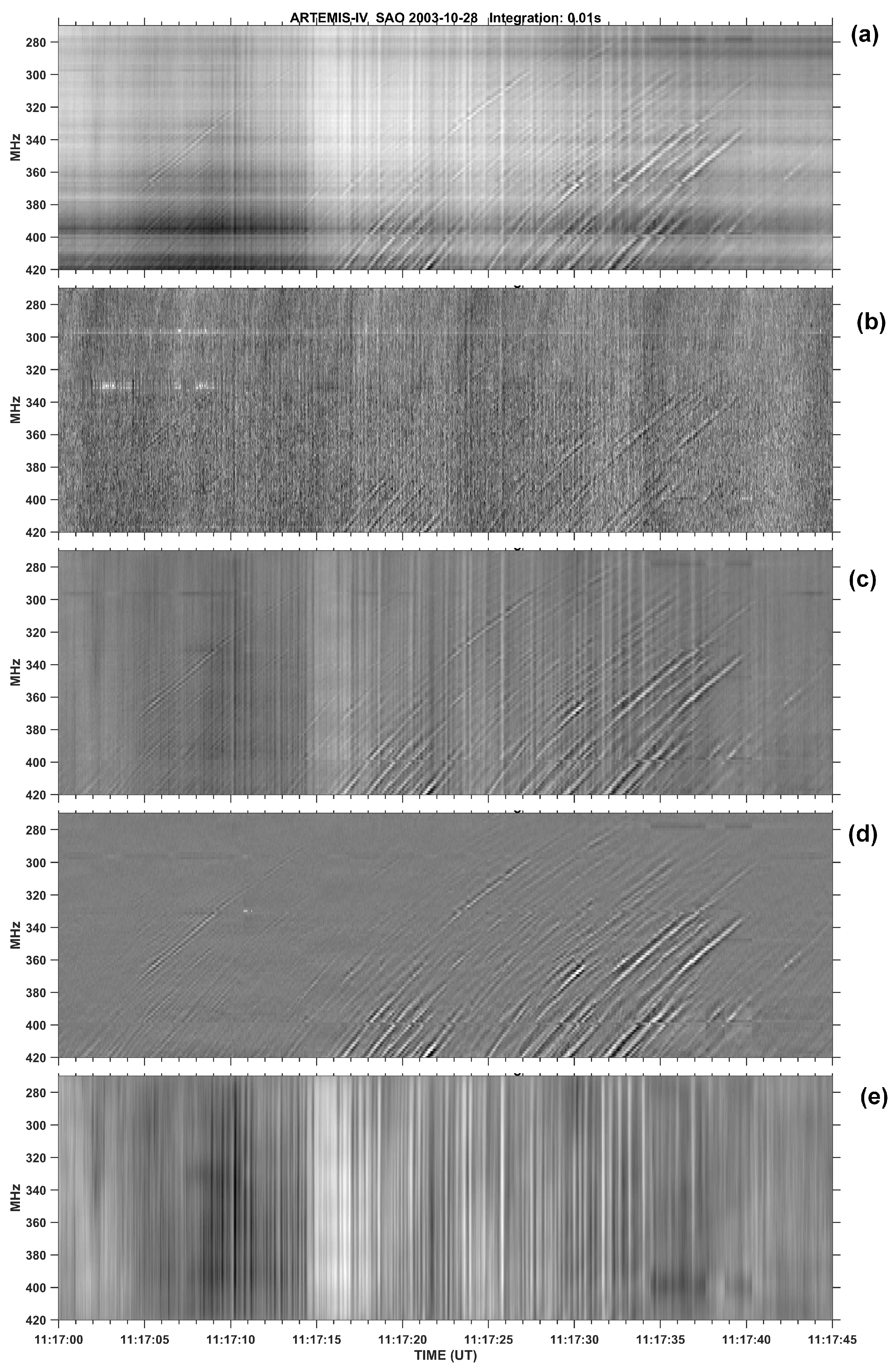
2.2.1. Enhancement of Fine Structures in Dynamic Spectra

As overlapping fine structures in dynamic spectra are embedded in the broad band and longer timescale continuum emission, we used the following techniques for their enhancement and separation:

• Suppression of the continuum background: It was performed by means of high-pass filtering in time, using either Gaussian filters or time derivatives (differential spectra), which enhanced fast time-varying spectral structures, such as pulsations, fibers, and zebras.
• Separation of overlapping fine structures: It was used mostly in the case of the type-IV data set. We used both high-pass and low-pass filters on dynamic spectra along the frequency axis. In this case, the high-pass filtering provides pulsation suppression and facilitates detecting fibers and similar structures, while the complementary low-pass filtering provides suppression of drifting structures, such as fibers (see [30,32] for a detailed description of this method).

An example of background suppression followed by separation of overlapping fine structure is presented in Figure 1.

2.2.2. Measurement of Bulk Parameters

Most of the fine structure bursts appear in groups and clusters. Their study necessitates the use of autocorrelation analysis of their intensity-time profiles or 2D autocorrelation function of the dynamic spectrum for the measurement of their bulk parameters, i.e., the duration at fixed frequency, the instantaneous bandwidth, the periodicity, and the frequency drift rate. The results need to be corroborated by direct measurement of parameters at subsets of clearly isolated fine structures. The fine-structure bursts of interest in this work, narrow-band bursts and intermediate-drift bursts, differ in the details dictating an adaptation of the methodology for each type, as described in this section.

In the case of spike groups, a 2D autocorrelation of the dynamic spectra provides the average spike duration, the frequency drift rate, and the bandwidth for a group of spikes. An example is shown in Figure 2. The results were validated by a semi-automatic evaluation of the duration and the instantaneous spectral width for the entire data set of narrow-band bursts. These were identified by inspection, and the width was determined by fitting the temporal and spectral profiles with a smooth curve. An example of the computation of the spectral and temporal width of a spike is presented in Figure 3. It shows part of the dynamic spectrum of a spike group and the measurement of the width of temporal and frequency profiles of an individual spike.

Similar to the method outlined above is the measurement of the spike duration and size in 1D NRH data through fitting of the positional and spectral profiles with Gaussians (Figure 4).

In the case of fiber bursts, which have a significant frequency extent, the characteristics of individual fibers were determined by means of a semi-automatic tracking algorithm which followed the peak of the flux from one frequency channel to the next [56,57]. This procedure was used in the measurement of the total bandwidth $\Delta f$, the total duration $\Delta t$ and the drift rate $df/dt$ of individual IDBs. In Figure 5a we show the track of individual fibers isolated from a group by this algorithm. In Figure 5b tracks as a function of difference from start time are plotted; the average track calculated from the fiber frequency drift (red line) is also plotted for comparison.

For the measurement of bulk parameters of fiber burst groups, 2D autocorrelation, cross-correlation, and 2D Fourier transform were used. The frequency-averaged 2D autocorrelation gave us the fiber duration, $\delta \tau$, computed from full width at half maximum (FWHM) of the central peak; the bandwidth, $\delta f$, of the emission was similarly obtained from the central peak of the time-averaged 2D autocorrelation (Figure 6d,e respectively). The fiber repetition rate (cadence) $T^{-1}$ within the group was calculated from the position of the first peak of the autocorrelation function on the time axis. Lastly, the bulk frequency drift rate, $df/dt$, of the group was estimated from the inclination of the 2D-autocorrelation function. The 2D-autocorrelation method gives only the average characteristics of the fiber bursts in a group, as opposed to the tracking algorithm mentioned above. However, it is fast, accurate, and easy to implement. Furthermore, the comparison with the tracking algorithm for individual bursts in our data set indicates that the values of the parameters of interest differ less than ∼10% between the two.

The fiber group drift rate as a function of frequency (and hence of time) was calculated by choosing a ten-channel spectral window and sliding it on the dynamic spectrum. The frequency drift was derived from the time shift of each channel with respect to the central one at each location of the sliding window, obtained by means of 1D cross-correlation (see Figure 7 for example); the characteristic curvature of the fiber burst in the dynamic spectrum is a result of the frequency drift rate decreasing with time.

When two or more fiber groups with different drift rates overlap on the dynamic spectra, the 2D Fourier transform was used for the estimation of the bulk frequency drift rate, $df/dt$, of each group as proposed by Tsitsipis et al. [58,59]. In this case, the 2D Fourier transform of the dynamic spectrum was converted to polar coordinates, ($s,\theta$). Then, the spectral power was plotted as a function of the polar angle, $\theta$, by integrating along the radius. In Figure 8, we show how this process separates well the different fiber groups in the inclination $\theta$ plot (panel b) and in the plot of the mean frequency drift rate, $df/dt$ (panel c).

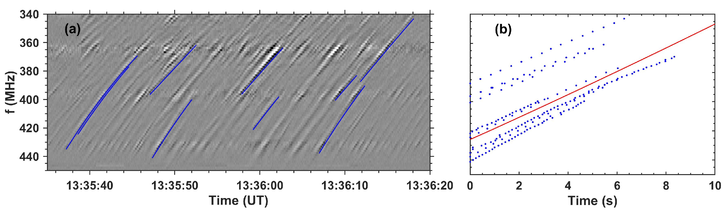
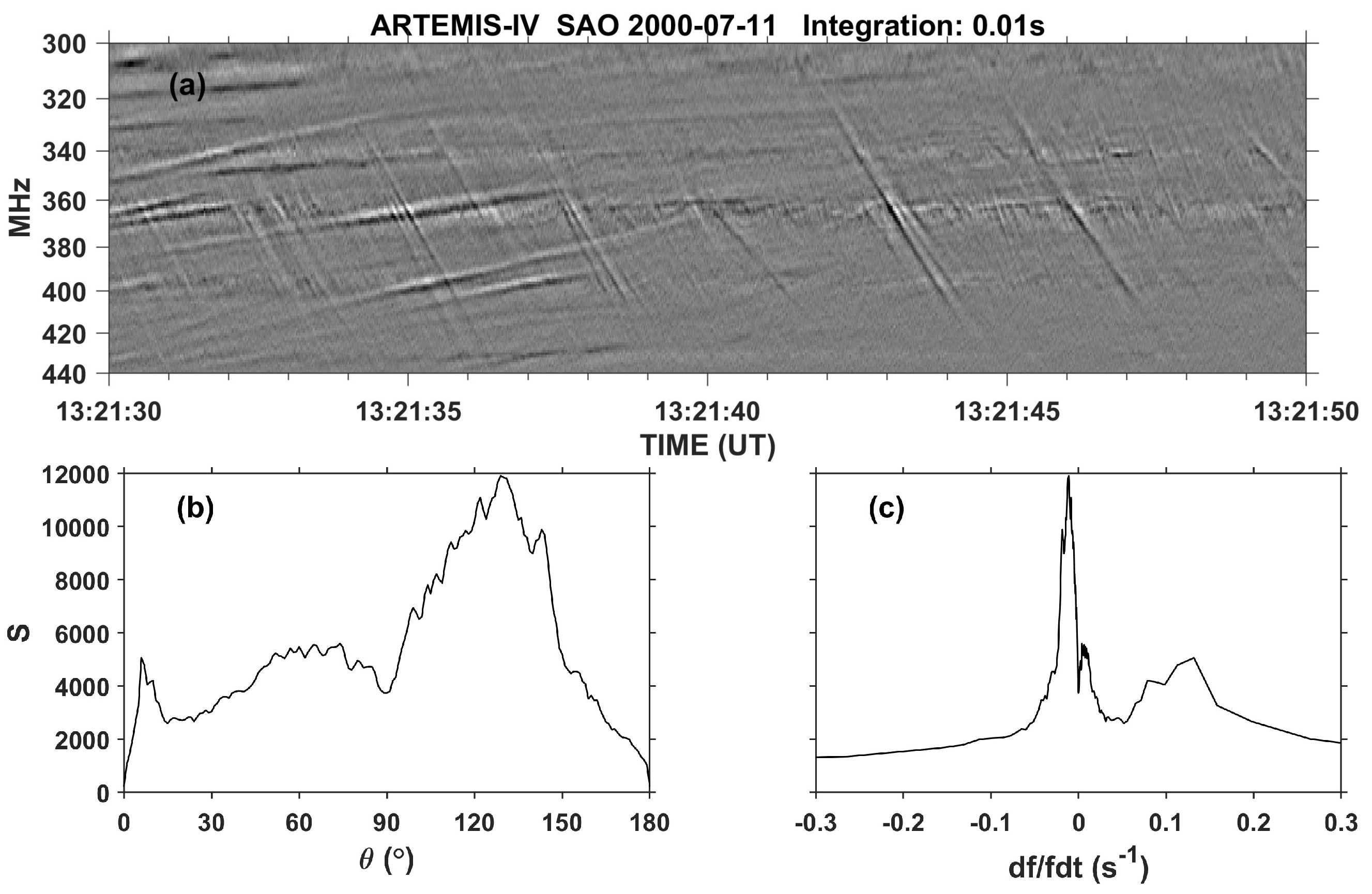
2.2.3. Drift Rate and Exciter Speed

In is well known, since the early days of solar radio astronomy, that the frequency drift rate in metric wavelengths is related to the speed of the exciter. Assuming that the radio emission is at the plasma frequency or the first harmonic, the emission frequency is associated with the electron density; hence, the speed of the burst exciter, $v_{exc}$, can be computed from the frequency drift rate, using the expression

$$v_{exc}=\frac{ds}{dt}=\frac{dz}{dt·cos\varphi }=\frac{H_f}{cos\varphi }\left(\frac{df}{fdt}\right)$$

(1)

where s is the distance along the path of the exciter, z is the height above the photosphere, and $\varphi$ is the angle between s and z. $H_f$ is the frequency scale height which is twice the density scale height, H; for an isothermal corona we have:

$$H_f=2H=\frac{2kT}{\mu m_p{g}_{\odot }}{\left(\frac{R}{R_{\odot }}\right)}^2$$

(2)

where k is the Boltzmann constant, T is the temperature, $\mu$ is the mean molecular weight (0.6 in the corona), $m_p$ is the proton mass, $g_{\odot }$ is the acceleration of gravity in the photosphere, and R (=z + $R_{\odot }$) the distance of the emission region from the center of the sun. Substituting numerical values we obtain

$$H_f\left[Mm\right]\approx 100T\left[MK\right]{\left(\frac{R}{R_{\odot }}\right)}^2$$

(3)

The vertical source size, $\Delta R$, is obtained by multiplying by the ambient coronal plasma frequency scale height, $H_f$, by the the relative bandwidth, $\delta f/f$.

$$\Delta R=H_f\left(\frac{\delta f}{f}\right)$$

(4)

For a given frequency, R can be computed from a coronal density model, yet this calculation is affected by ambiguities introduced by variations in the ambient medium properties and the model selection. A thorough discourse on coronal density models has been provided by Pohjolainen et al. [60,61].

In our fine-structure calculations [54,55,57,62], we have used the twofold Newkirk [63] model and the hybrid model of Vršnak et al. [64]. These well-established quiet-Sun models have frequency scale heights which are almost constant within the SAO frequency range and not too different from the barometric scale height at $T\approx 1.5$ MK. For the former, we have $H_f=140\times {10}^3$ km for emission at the fundamental and $190\times {10}^3$ km at the harmonic, and for the latter $H_f=100\times {10}^3$ km for emission at the fundamental and $150\times {10}^3$ km at the harmonic. Under the circumstances, an average frequency scale height of $H_f\approx 120\times {10}^3$ km at the fundamental and $H_f\approx 170\times {10}^3$ km at the harmonic was deemed acceptable.

The frequency drift rate from which the speed of the exciter is computed has a natural upper limit corresponding to the speed of light, c. An approximate upper bound of the relative frequency drift rate may be derived for both the fundamental (F) and the harmonic (H) from Equation (1):

$${\left(\frac{df}{fdt}\right)}_{\max }^{\mathrm{F}}\approx \left(\frac{c}{H_f}\right)\approx 2.5{\mathrm{s}}^{-1},{\left(\frac{df}{fdt}\right)}_{\max }^{\mathrm{H}}\approx 1.75{\mathrm{s}}^{-1}$$

(5)

When frequency drift rates beyond the limits set by Equation (5) are measured, they are referred to as “superluminal” exciter apparent motion; this observational contradiction may be resolved in two ways: First, the local scale height might be less than predicted by quiet-Sun models. Secondly, following Poquerusse [65], Klassen et al. [66], Benz et al. [67], a geometric correction which accounts for the radio emission “time of flight” needs be applied to both the measured speed, $V_m$, and the relative frequency apparent drift rate, ${(df/fdt)}_m$:

$$V=V_m·{\left(1+\frac{V_m}{ccos\theta }\right)}^{-1}\iff \left(\frac{df}{fdt}\right)={\left(\frac{df}{fdt}\right)}_m·{\left(1+\frac{V_m}{ccos\theta }\right)}^{-1}$$

(6)

where V is the actual exciter speed and $\theta$ is the the angle between the exciter path and the line of sight. Thus, for an exciter moving outwards in the radial direction, this factor is unity at the solar limb, but at the center of the disk and for an exciter speed of 0.7c, it is ≈4. The effect of the correction factor is quite pronounced in the case of exciter speeds exceeding $c/10$. This is often the case with bursts of the type-III family, drifting narrow-band structures, and pulsations

Alternative interpretations of apparent superluminal velocities have been provided in terms of multiple sources (see Section 6.2.2 below and [68]) as well as in terms of geometric effects [38].

3. Fine-Structure Classification in the Metric Wavelength Range

The criteria used in the development a fine-structure classification scheme were based on the morphology of the fine structure on dynamic spectra from the ARTEMIS-IV/JLS/SAO receiver. The basic data set was in the metric wavelength range, yet we have strived for a flexible scheme capable to accommodate different fine structure frequency bands, including the highly complex structures of the microwave range. The results are consistent with the Ondrejov catalogue [23,24,26], which was based on data in the 0.8–2.0 GHz range. However, at variance with previous attempts, we opted for a more structured approach adopting two-level classification. The fine structures were thus allocated into five basic classes, corresponding to coarse-grained spectral features. Each basic class was further divided in two or more subclasses based on the finer details of the spectral features [27]. This two-level hierarchical arrangement serves the diversity of the microwave–decimetric bursts which exceeds that of their counterparts in the meter range and below [69]. Details of the two-level scheme are given in the following Section 3.1, Section 3.2, Section 3.3, Section 3.4 and Section 3.5. In the classification process, statistical results were also obtained regarding the association of the various types with the various phases of the flare/CME phenomenon, which could be useful in understanding details of the evolution of the solar energetic phenomena through their radio signatures.

3.1. Featureless Broadband or Diffuse Continuum

This class includes both diffuse segments of type-IV bursts and radio emissions of smaller bandwidth and duration, such as slowly drifting bursts and patches. Intensity variations within the smooth periods of the recorded type-IV bursts might qualify as patches too. In Bouratzis et al. [27], long periods of broadband continuum were found to overlap in time with the SXR emission and with embedded intermittent periods of the fine structure mentioned in Section 3.2, Section 3.3, Section 3.4 and Section 3.5 below. The smooth periods devoid of fine structure varied between 0% and 60% of the type-IV continuum duration; the relatively longer smooth periods were found to increase with the duration of the type-IV burst. Although periods of featureless diffuse continuum have been recorded in abundance in the past, our data suggest that fine structure may still be detected at sufficiently high resolution and sensitivity.

3.2. Pulsating Structures

The dynamic spectra pulsating structures appear either as drifting or stationary (see [17] for a review); the shortest groups of these structures with durations ∼10 s are known as isolated broadband pulses in [23,24,26]. They are considered as the result of quasi-periodic acceleration episodes in reconnecting current sheets [7]. The ensuing kinetic plasma instabilities and the corresponding energetic electron populations are thought to produce the characteristic radio signature which are known as quasi-periodic pulsations (QPPs). In the microwave frequency range (0.8–2.0 GHz), drifting QPPs are thought to be among the possible flare radio precursors as they were found to precede the flare onset by ∼1–4 min [70].

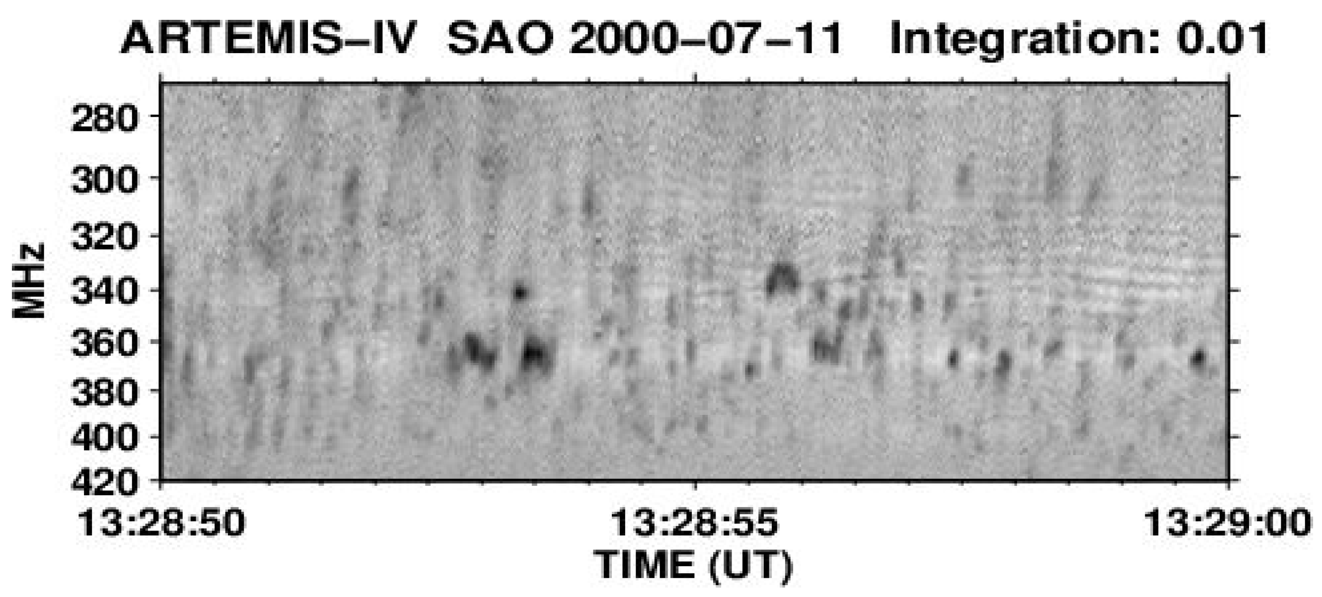
3.3. Narrow-Band Bursts

The signatures of small-scale acceleration episodes (see review by Nindos et al. [10]) manifest themselves as narrow-band bursts of the type-III family: spikes, dots, and subsecond patches [71], depending on their shape in the dynamic spectra. Part of the same family are the III(U) and III(J) narrow-band bursts [25,72] and the supershort structures (SSSs) found embedded in the metric solar type-IV continua [73,74]. The high time-resolution of the SAO receiver made the morphological distinction possible between a large number of different narrow-band structures of the ARTEMIS-IV/JLS data set, such as narrow-band J or U bursts, and the unusual inverted U burst. The duration and bandwidth distributions, however, did not show any clear separation in groups (see

Table A1. Durations and spectral widths of the radio spikes observed in the 19 MHz to 7.5 GHz band (derived from Table 1 of Da̧browski et al. [197] augmented with additional data from [54,62,198,199]).

Freq. [GHz]	Duration [ms]	Time Res. [ms]	Width [MHz]	Freq. Res. [MHz]	Reference
0.011	800.0	100	0.025	1	Shevchuk et al. [199]
0.019	1400.0	100	0.060	1	Melnik et al. [198]
0.024	1000.0	100	0.060	1	Melnik et al. [198]
0.029	800.0	100	0.080	1	Melnik et al. [198]
0.040	410.0	100	0.080	1	Shevchuk et al. [199]
0.330	–	–	9.900	1–10	Benz et al. [200]
0.350	100.0	10	10.00	1.6	Bouratzis et al. [54]
0.350	96.0	10	10.00	1.4	Armatas et al. [62]
0.350	–	–	4.800	1	Messmer and Benz [201]
0.360	–	–	7.320	1	Csillaghy and Benz [151]
0.360	73.0	2	–	1	Guedel and Benz [148]
0.400	4–30	1 & 10	∼20	–	Magdalenić et al. [73]
0.470	41.0	0.5	–	3	Guedel and Benz [148]
0.480	–	–	12.600	6	Csillaghy and Benz [151]
0.600	–	100	∼2	0.061	Benz et al. [67]
0.730	20.0	10	–	10	Guedel and Benz [148]
0.770	20.0	2	–	10	Guedel and Benz [148]
0.830	–	–	7.040	1	Csillaghy and Benz [151]
0.870	19.0	10	–	10	Guedel and Benz [148]
0.940	–	–	7.500	1	Messmer and Benz [201]
1.010	17.0	10	–	10	Guedel and Benz [148]
1.160	–	–	49.500	14	Csillaghy and Benz [151]
1.340	–	–	17.000	10	Csillaghy and Benz [151]
1.420	2.0	1	–	–	Wang and Xie [202]
1.420	9.0	1 & 10	–	–	Mészárosová et al. [149]
1.690	–	–	32.300	10	Csillaghy and Benz [151]
2.000	1.3	1	–	–	Wang and Xie [202]
2.700	5.1	1 & 10	–	–	Mészárosová et al. [149]
2.800	–	–	10.800	10	Csillaghy and Benz [151]
2.840	13.2	1	–	–	Wang and Xie [202]
3.200	14.0	8	–	10	Chernov et al. [203]
3.200	42.7	8	117.300	10	Wang and Xie [202]
3.200	8–36	8	20–110	10	Wang et al. [204]
5.250	–	5	∼30	10	Rozhansky et al. [150]
7.300	∼100	100	120.000	10	Benz et al. [205]
7.400	–	–	48.700	11	Csillaghy and Benz [151]

of the Appendix A). The narrow-band bursts occasionally comprise the “superfine structure” (or “hypefine structure”) of various type of bursts as already mentioned in Section 1. Examples of radio bursts formed from spike chains are type-III bursts in the 1–2 GHz range [75], pulsating structures in the 2.6–2.8 GHz range [76], etc. Furthermore, the narrow-band bursts are part of both the type-II and the type-IV-associated fine structure; as such, they are discussed further in the following Section 4 and Section 5.1. We note that type-I bursts, superposed on type-I continua (noise storms) at metric frequencies (See [77]), also have small duration and bandwidth and spike-like dynamic spectra. Their duration and bandwidth is close to the type-II-associated spike-like bursts and the type-IV-associated spikes observed in the same frequency range [78,79]; high-resolution observations by Iwai et al. [80] corroborate this similarity.

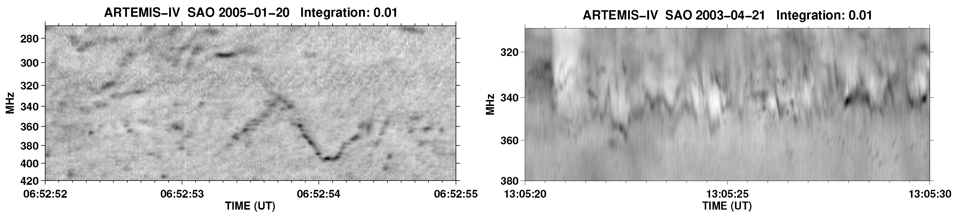
3.4. Intermediate-Drift Bursts

The intermediate-drift bursts are characterized by their drifting stripe-like form, whose drift rate exceeds that of the type-II bursts but does not reach the type-IIIs and their absorbtion ridge. They include the typical fibers [81,82,83,84,85], the narrow-band rope-like fibers [86,87,88,89], the narrow-band fibers, and the fast drift fibers (FDBs). The fiber bursts are mainly detected drifting along coronal magnetic structures and, in particular, postflare loops. In the metric wavelengths, they usually appear some minutes after the first energy release marked by the first HXR or microwave peak (see, for example [27], Figure 9). The intermediate-drift burst radio emission has been interpreted as the result of whistler–Langmuir [82,83,84] or Alfvén–Langmuir wave interaction [90], based on their characteristic drifting stripes in emission and absorption; they provide, thus, a valuable radio–diagnostic of Solar Coronal Magnetic Fields [91,92]. The theory of whistler (or Alfvén) origin stipulates a three-wave coupling process ($l+w\to t$ or $l+A\to t$), where whistlers (w) or Alfvén (A) coalesce with the Langmuir waves (l) of the type-IV background, resulting in transverse wave emission (t). The three wave interaction ($l+w\to t$ or $l+A\to t$) depletes the background Langmuir wave energy, resulting in the absorption ridge at the the plasma frequency (low-frequency side of the fiber) and produces enhanced emission at the sum of the frequencies of the interacting waves. A different approach was presented recently by Ni et al. [93,94], who considered the production of fundamental electromagnetic radiation (ordinary mode, O) at the plasma frequency induced by the resonant coupling of Z-mode and whistler (w) waves ($Z+w\to O$); this might offer an alternative IDB interpretation. In Section 6 below, where the intermediate-drift bursts are described in more detail, we posit that the $l+w\to t$ interaction is the dominant fiber emission process at the metric wavelength range. The Alfvén–Langmuir wave interaction case, on the other hand, is improbable as it requires too high a magnetic field at the coronal height corresponding to this range.

3.5. Emission Bands

The zebra family is the the emission bands and it shows significant diversity, including the classic or pulsation-superposed zebra patterns, the fiber-associated zebras [88,95], and the zebras with a drifting emission envelope [96]. The corresponding emission mechanism interpretations vary from double plasma resonance [97,98], Bernstein modes, or plasma waves trapped in resonators, and more (see Nindos et al. [10], Chernov [95]). The rare lace-burst, first reported by Karlický et al. [99], is also member of the zebra family; its emission has been attributed to the double plasma resonance [6,100,101], and observational evidence in support of this interpretation has been provided by Chen et al. [102]. The zebra bursts exhibit stripes in emission and absorption comparable to the fibers, and hence they provide an additional radio–diagnostic for Solar Coronal Magnetic Fields [91,92].

Some uncommon band structures from the metric–decimetric frequency range have been also included in this class:

• A single-emission band, designated as evolving emission line (EEL), first reported by Chernov et al. [103] in the 350–450 MHz frequency range, at the low-frequency cutoff of a pulsating structure, and by Fu et al. [25] and Ning et al. [104] in the GHz range is included in this class, although the emission mechanism appears to be somewhat different from the zebras. After Chernov et al. [103], the observed EEL was the result of electrostatic maser at double plasma resonance.
• Some “serpentine” single-emission bands recorded in the ∼5 GHz frequency and designated as a “quasi-periodic drifting” structure ([25], Figure 9), or “M-shaped structure” ([105], Figure 3) may be classified, either as emission bands or as narrow-band bursts of the type-III family (M-Bursts).
• A structure detected at about 1416–1420 MHz by Oberoi et al. [106]. It consists of a group of short 2–4 ms parallel stripes with a relative delay with decreasing frequency. The total duration of the group is about 16 ms. Due to the band structure, this burst may be considered as a group of emission bands; the short time scale and frequency bandwidth of these bands, however, show some similarity of this burst to narrow-band burst chains.

4. Type-IV-Associated Narrow-Band Bursts (Spikes)

The narrow-band bursts are characterized by very small duration (∼50 ms in the metric frequency range) and bandwidth ($\delta lnf\approx$ 1–2%). They often appear embedded in the continuum background of the type-IV radio bursts. In the lower frequency range (metric and lower wavelengths), the narrow-band bursts are thought to be signatures of small-scale acceleration episodes which induce enhanced Langmuir waves by means of bump-on-tail instability. These in turn are converted into electromagnetic radiation in the fundamental and the first harmonic of the local plasma frequency. In the microwave range, on the other hand, they are interpreted as gyrosynchrotrons or electron cyclotron masers (see [107,108,109]). In this section, we summarize our results, presented in Bouratzis et al. [54].

4.1. Characteristics of Individual Bursts and Chains

The characteristic parameters of both individual narrow-band bursts and chains, such as their duration, $\delta \tau$; bandwidth, $\delta f$; and drift rate, $df/dt$, were measured using the methods presented in Section 2.2. For the individual spikes, the semiautomatic algorithm described in Section 2.2 was used on a selection of 11,579 narrow-band bursts (see example in Figure 3). In Figure 9a,b, we present histograms of the duration and the bandwidth of the narrow-band structures. For comparison, the spike durations and spectral widths in the 11 MHz–7.40 GHz range, published in a number of articles, are given in Table A1.

The individual spike characteristics, such as normalized (or relative) bandwidth, $\delta f/f$, and duration, $\delta \tau$, were found to be on the average 2% (≈7.8 MHz) and 100 ms, respectively, with the bandwidth tending to increase with duration. The observed relative bandwidth corresponds to a spike vertical size of about 2.4–3.4 $\times {10}^3$ km (see Equation (4)). A small number (less than 1% of our data sample) of outliers were found, with $\delta f/f\approx 0.2$. These corresponded to the very rare broadband spikes, first reported in [110] in the 175–235 MHz range, and are shown in the left panel of Figure 10. In the right panel of the same figure we show a cluster of typical narrow-band structures for comparison.

The spike frequency drift rate, $df/dt$, was measured on a sample of 295 spikes, some of which showed positive (sunward) and some negative (outbound) drifts (see for example Figure 11) with average rates of 506 MHz s${}^{-1}$ and −390 MHz s${}^{-1}$ respectively; these correspond to relative frequency drifts of 1.43 s${}^{-1}$ and −1.12 s${}^{-1}$. In addition to the drifting spikes, a number of spikes with non measurable drift was also recorded.

A number of parallel chains were found, where the spikes of the low-frequency chain had negative drift, while the corresponding spikes of the high frequency chain had positive drift (Figure 11, left). These “bi-directional spikes” appear to be the signatures of a sequence of small-scale X-reconnection events. The small number of the observations of such chains is probably due to the fact that they are quite difficult to distinguish within spike clusters. Moreover, as already mentioned in Section 3.3, narrow-band bursts have been recorded on dynamic spectra in diverse forms, such as type-III, -III(U), and -III(J) narrow-band bursts, spikes, dots, and subsecond patches and supershort structures (SSSs) [25,71,72,73,74]. Examples are shown in Figure 12.

In dynamic spectra, as a rule, spike bursts tend to cluster close to one another in time or in frequency. When large groups of individual spikes are grouped within a very short time interval (≲1 s) over a wide frequency range, the clusters are labeled as columns [111]. In our data, the reverse (sunward) drifting columns had an average group drift rate of about 517 MHz s${}^{-1}$ (logarithmic drift rate $df/fdt\approx 1.36$ s${}^{-1}$); the negative (outbound) drifting columns, on the other hand, had $df/fdt\approx 3.25$ s${}^{-1}$ ($-1260$ MHz s${}^{-1}$). The drift rate of the latter is similar to that of the fastest member of the type-III family (the type-IIId bursts); these were found to have a drift rate of about $-1500$ MHz s${}^{-1}$ in the 500–100 MHz frequency range by Poquerusse [65]. The outbound columns are also similar to the fastest of the chains of dot-like structures reported by Sawant et al. [112] in the frequency range 1000 to 2000 MHz, with drift rates in the −180 to −1200 MHz s${}^{-1}$ range. These apparent drift rates correspond to “superluminal” exciter speeds (for example a $3.25$ s${}^{-1}$ drift corresponds to exciter speed equal to $1.3$c). As discussed in Section 2.2.3, the application of the geometrical correction at the center of the disk reduces the exciter speed to $0.6$c.

Spike chains represent another interesting class of clusters. Their group frequency drift is mostly negative, $df/fdt\approx -0.021$, with only a few exhibiting reverse drift at a rate of $df/fdt\approx 0.033$ s${}^{-1}$ and even fewer with zero drift. In our data set, the average chain duration was in the 2–20 s range. The chain group drift rate is similar to the drift of fiber bursts recorded at the same time as the chain; an example is presented in Figure 13.

Some unusual kinds of spike groups were detected by ARTEMIS-IV/JLS. In dynamic spectra, these groups appear in the form of N bursts [113] or in the form of lace bursts [99], composed of sequences of spikes. An example of N burst-like pattern is presented in the left panel of Figure 14; it consists of three branches with each branch formed by a fast spike chain. Their duration is about 1–3 s and the relative drift rate of each component is ∼0.4 s${}^{-1}$, similar to the drift rate of the type-III(N) bursts. An example of lace burst-like patterns is presented in the right panel of Figure 14. Similar results for superfine structures were reported in [114,115,116] for zebra bursts in the microwave frequency range.

The theoretical interpretation of the superfine structures of zebra and laces by Bárta and Karlický [117,118], Bárta et al. [119] is based on the combined effects of the double resonance emission mechanism and the background turbulence. The lace and zebra emission bands are expected to form at positions where the upper hybrid plasma frequency equals a low harmonic of the electron cyclotron frequency. The spike superfine structure results, in turn, from the cascade of the background turbulence to small spatial scales.

Both the observations and theory suggest that it is possible that a significant part of the fine-structure bursts may be resolved in spikes as higher resolution observations become available. This assertion has been corroborated by very-high-resolution (80 $\mathsf{\mu }$s) observations of spikes in the 1352–1490 MHz frequency range with 46 channels and 3MHz frequency resolution by Dabrowski and Kus [111], Dąbrowski et al. [120]. These spikes were partitioned into bursts “with internal structure” and bursts “without”, where the internal structure was distingushed by local peaks, within the time and frequency limits of the spike. The question whether a real internal structure exists or if it is a case of very short chains of tightly packed spikes is, to the best of our knowledge, open, but it still underlines the importance of high frequency and time resolution observations.

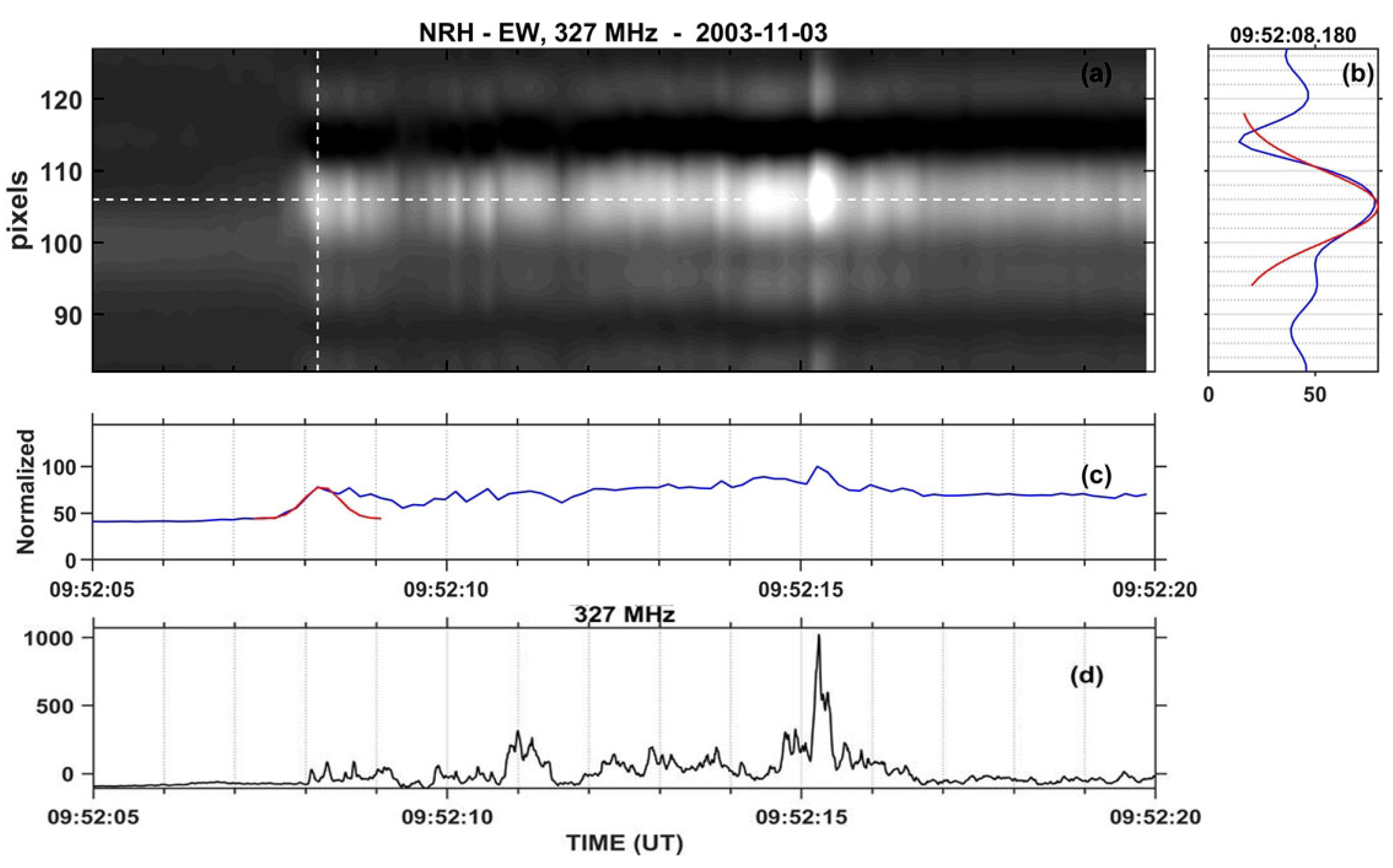
4.2. Spectral Imaging of Spikes with ARTEMIS-IV/JLS & NRH

In this section, we present spike observations during the event of 21 April 2003 (SOL2003-04-21T13:07:30), recorded by the ARTEMIS-IV/JLS and the NRH. This event was associated with a GOES M2.8 class flare in NOAA AR10338 at N18E02 and a CME (see Figures 13 and 14 of Bouratzis et al. [54]). During the rise phase of the microwave emission, a large number of type-III bursts appeared which extended into interplanetary space (see https://secchirh.obspm.fr/ (accessed on 23 July 2023)). Two type-II bursts with fundamental-harmonic structure, a type-IV continuum and a moving type-IV were also recorded as parts of the same event.

Intense spike emission was observed during the early phase of the event with a duration of about 23 s from 13:03:22 to 13:03:45 UT. Several spikes occurred at the NRH frequencies that were within the SAO spectral range, and practically all of them were detectable in the NRH 1D mages. The spikes were on top of a slowly varying background NRH source at all frequencies (see Figure 15); they were smaller and often displaced with respect to that background, forming preferentially at its periphery. Figure 16 shows contour plots of 1D intensity during the same time interval, after high-pass filtering in time aiming at suppressing the background. The figure shows that most spikes are smaller than the background source, and many of them are displaced with respect to it, always remaining within its half width.

2D NRH difference images between some prominent spikes and the nearest background image were used to measure spike parameters, with the average values given in

Table 1. Average parameters of spikes for the 21 April 2003 event. From Table 3 of Bouratzis et al. [54], reproduced with permission.

Parameter	327 MHz	411 MHz	432 MHz
Number of spikes	8	15	13
Shift, ${}^{″}$	35	11	18
Spike $T_B$, 10${}^8$ K	1.2	1.9	1.6
$T_B/T_b$ ratio, spikes/background	0.57	0.85	0.66
Area ratio from 2D	0.86	0.81	0.83
Area ratio from 1D	0.32	0.50	0.41
Size from 1D, in ${}^{″}$	86	82	72

; the brightness temperature of the spikes was 1.2 to $1.9\times {10}^8$ K, i.e., 0.5 to $3.5\times {10}^8$ K above that of the background source. The average temperature ratio was found to be ≈0.7. The area of spike sources was about 80% that of the background, which is double the area ratio computed from the 1D NRH recordings due to the better resolution of the 1D images, as discussed in Section 2.2. The spikes, on average, were shifted by 10${}^{″}$–30${}^{″}$ with respect to the background; the NRH resolution exceeds the shift, yet it may be confirmed from the 1D images of Figure 15 and Figure 16, which indicate that spikes are often at the flanks of the slowly varying source.

We note that the observed brightness temperature, $T_B$, is a lower limit to the true one, due to the limitations of the NRH spatial resolution, which resulted in a measured spike source extent greater than the actual, as well as due to possible scattering effects. We further note that these results ($T_B\approx 2\times {10}^8$ K) are significantly lower than similar calculations by Benz [78], which give $T_B\approx 2\times {10}^{15}$ K and reasonably so, as this author used a much smaller source size, ≈0.3${}^{″}$, based on the spike duration and the speed of light. In any case, the measured brightness temperature of $T_B\approx 2\times {10}^8$ K is much greater than that of the quiet Sun (4–6 ${10}^5$ K, see Lantos et al. [121], Lantos [122]) and precludes thermal emission but corroborates non-thermal or coherent emission mechanisms.

The above analysis suggests that the spikes are additional emissions, apparently from small-scale reconnection events within or very close to the background source, rather than fluctuations of the background.

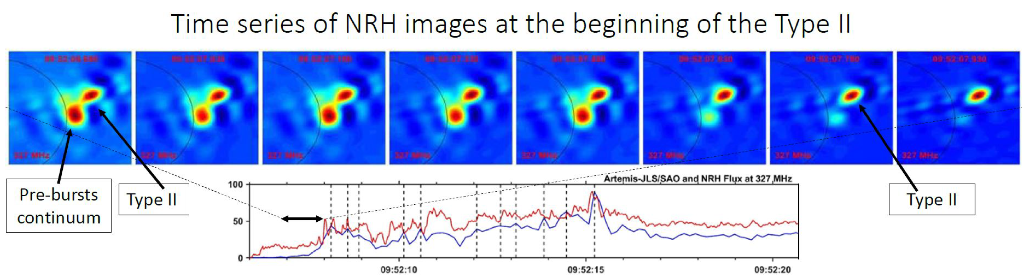
5. Type-II-Associated Fine Structure

The type-II bursts are the radio signatures of MHD shocks in the solar corona, drifting [123,124,125,126] or stationary [7,127,128,129]. The latter have been interpreted [7,127,128,129] as terminationshocks. It is possible that a number of them are due to the coronal conditions as is the case of a narrow CME shock front which propagates and eventually expands within a streamer [130] forming a stationary type-II. Type-II bursts sometimes show a split in two lanes with a small frequency offset of ≈f/8–f/4 [64,131,132,133]. The shock-accelerated suprathermal electrons drive the emission mechanisms of both the type-II bursts [134,135] and the associated fine structure. The fine structure is quite diverse including, but not restricted to, herringbone bursts [136,137,138,139,140,141], low-drift fiber-like bursts [142,143] and narrow-band bursts [136,144,145,146].

In this section, we describe the results of the study of four well-observed type-II events (see Armatas et al. [55,62]); emphasis is placed on the 3 November 2003 Event (SOL2003-11-03T09:43:20), for which both ARTEMIS-IV/JLS/SAO and NRH observations were available.

5.1. Overview of the 3 November 2003 Event (SOL2003-11-03T09:43:20)

The event was selected to illustrate the basic spectral and spatial characteristics of the type-II-associated FS bursts. The bursts recorded on the top panel of Figure 17 by the ASG include a type-II exhibiting fundamental-harmonic structure preceded by groups of type-III bursts and followed by a type-IV continuum. The dynamic spectrum obtained at high time-resolution by the SAO revealed a variety of fine structures, described in detail in Figure 5 of Armatas et al. [62]. The fine structure is enhanced by means of high-pass filtering (middle panel of the Figure 17) and in the differential spectrum (lower panel).

Among the fine-structure bursts, chains of spike-like dots, quite similar to the type-IV-associated spikes stand out (better seen in the top panel of Figure 18). We note that an additional type of fine structure was recorded, consisting of groups of almost vertical structures, looking more like pulsations rather than herringbones. These appeared at frequencies higher than the type-II lanes, had negative (anti-sunward) drift, and terminated at the spike chains.

As already mentioned in Section 4.1, the basic characteristic of the individual spike bursts are their very short duration (∼100 ms in the metric frequency range) and bandwidth (∼1–2%).

An important question is whether these spike-like structures are similar to the type-IV-associated spikes exposed in previous sections. In the case of type-II-associated spikes, the tendency to form chains is considerably more pronounced than the type-IV-associated spikes discussed in Section 4. Multiple spike-like chains were detected on all four events of our sample. These chains drifted in frequency, approximately parallel to one another, forming emission lanes, apparently portraying different regions of the shock front. We note that the spike emission constitutes a significant part of the type-II radio emission.

The average duration of the type-II-associated spike-like structures was found to be 96 ± 54 ms and the average relative bandwidth 1.7 ± 0.5%, which are the same as the characteristic parameters of the type-IV-associated spikes within the ARTEMIS-IV/JLS/SAO resolution.

5.2. Comparison of Spectral and Imaging Data

Due to the frequency drift of the type-II lanes, only a small number of the spike chains presented in Figure 18 were detectable in the fixed frequency channels of the NRH. Furthermore, the NRH time resolution of 150 ms is significantly lower than the 10 ms resolution of the ARTEMIS/JLS SAO receiver; therefore, individual spikes closely placed in time recorded by the SAO cannot be resolved by the NRH.

Important information on the type-II burst source positions and structure and the pre-existing continuum source was provided by the NRH 2D images. Figure 19 shows a sequence of 327.0 MHz images at the onset of the type-II emission. We note that the projected location of the pre-type-II emission was 0.1$R_{\odot }$ above the west limb, whereas the type-II source was displaced by about 5.3${}^{\prime }$ (0.3$R_{\odot }$), and their position angles differed by 13${}^{\circ }$.

The position difference between the pre-burst and burst sources during the full event is shown in the left panel of Figure 20, where the source positions at 236.6 MHz were included This frequency was below the SAO range, yet the ASG recordings (top panels of Figure 17) depict clearly the type-II front; furthermore the NRH images at 236.6 MHz show a multitude of short timescale structures, some of which might be isolated spikes or spike groups. At 236.6 MHz, the sources of the continuum and the type-II were above the corresponding 327 MHz sources: the burst sources were displaced by about 6.4${}^{\prime }$, or 0.4$R_{\odot }$ with respect to the continuum sources, and their position angles are almost identical. Similar positions of the emission sources are shown in Figure 7 of Dauphin et al. [147].

An important question is whether the spike emission is at the same location as the emission between spikes or, as in the case with type-IV-associated spikes, it is located at the periphery of the background emission. To this end, we plot in the middle panel of Figure 20 the brightness temperature, position, and size of the 327 MHz burst sources as a function of time; asterisks mark the spike sources. The right panel of the same figure shows the source positions on the plane of the sky, with red asterisks marking again the spikes. Soon after the initial rise of $T_b$ at 09:52:08 UT, the position of most sources falls on a straight line, reflecting the outbound motion of the type-II front. Spikes 1–9 also fall along this line, whereas spikes 10–12 do not; the latter are part of a different spike chain, apparently associated with a different part of the shock front than the one which produced spikes 1–9.

The results presented above demonstrate the rather insignificant position difference between spike and inter-spike emission. As the spike-like bursts appear to be associated with the entire emitting region, they constitute the principal radio signature of the MHD shock type-II radio emission. Thus, the spike-chains delineate the shock front emission, which in low-resolution dynamic spectra appears continuous. The prevalence of spike-like burst chains virtually forming the type-II fronts suggests some type of organized structure in the small-scale reconnection driving the energetic electrons which excite the spike bursts.

5.3. TypeII- and Type IV-Associated Narrow-Band Bursts: Similarities & Differences

In this section, we compare the type-II and type-IV-associated narrow-band bursts, based on the average parameters of individual bursts, on the structure of burst groups and chains, and on their relationship to the associated type-II and type-IV bursts. The similarity of the characteristics between the type-II-associated spike-like structures and the type-IV-associated spikes provide evidence of the emission process relationship. In

Table 2. Parameters of type-II-associated spike-like bursts and type-IV-associated spikes. Adapted from Table 1 of [62].

Parameter	Type-II Spike-like Bursts	Type-IV Spikes
Number of spikes	642	11,579
Number of spikes/event 160	330
Duration (ms)
Average	96	100
Standard deviation	54	66
Relative bandwidth
Average	1.7%	2.0%
Standard deviation	0.5%	1.1%

, we compare the average parameters (duration and relative bandwidth) of the two spike categories; these appear quite similar, allowing for the standard deviation of the samples. The difference in spike counts per event stems from type-IV events having significantly longer duration than type-II bursts, within the same frequency range.

The duration–frequency and instantaneous bandwidth–frequency relations for spikes are usually expressed by phenomenological power laws of the form $\delta \tau \propto f^a$, ($a\approx 1.32$) [148,149,150] and $\delta f\propto 0.66f^{0.42}$ [151]. In Figure 21, plots of these two power laws are presented, together with the data in the 0.3–3 GHz range from Table A1. We note that average values obtained with the SAO are near the values expected from the empirical relations.

The results in Table 1 and Table 2, as well as Figure 21, show the similarities between type-IV-associated narrow-band bursts and their type-II-associated counterparts, providing strong evidence for a common emission mechanism. The principal differences between the two are: (a) the form of spike groups in the case of type-IV-associated spikes is quite diverse (see Section 4.1), comprising of clusters of isolated spikes and chains of consecutive spikes with widely varying group drift rate. The type-II-associated spike groups, in contrast, form chains drifting at a similar to the type-II burst rate. (b) Type-IV spikes form at the periphery of the background continuum (see Section 4.2), whereas the type-II-associated spikes did not exhibit any substantial position difference with respect to the inter-spike emission, thus appearing to be related to the entire emitting region of the shock front.

6. Type IV-Associated Intermediate-Drift Bursts (Fibers)

The basic characteristics and the proposed emission mechanisms of fiber bursts were discussed in Section 3.4 and will not be repeated here. In this section we will discusse our spectral and imaging results, obtained with ARTEMIS-JLS and the NRH (see [57,68]). These include classification, statistics, estimates of the magnetic field, and spatial structure.

6.1. Information from Dynamic Spectra

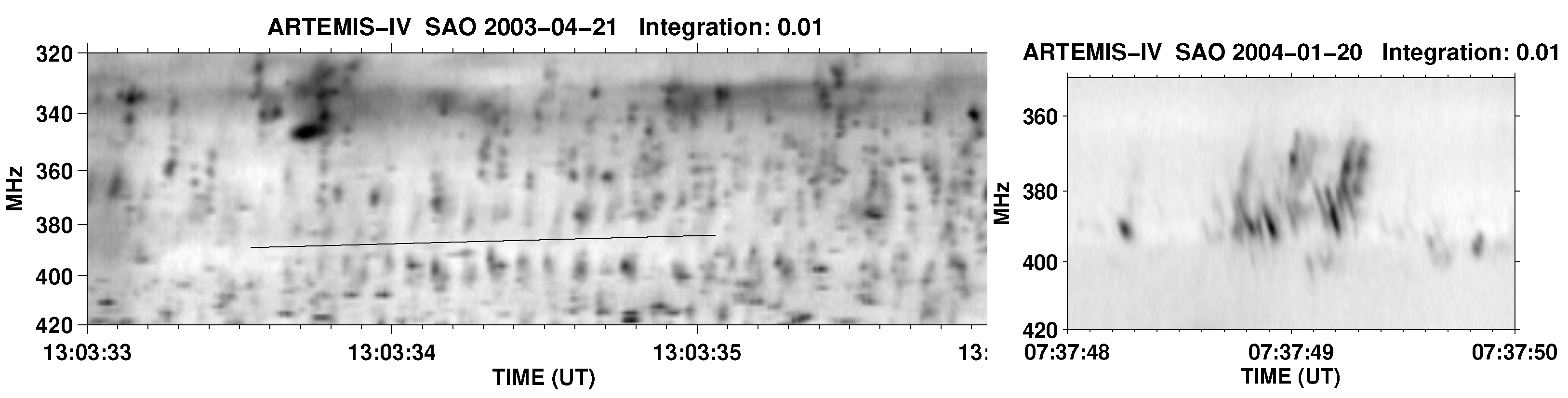
6.1.1. Fiber Burst Classes

Based on the particulars of the emission–absorption ridge combinations in the dynamic spectra, the fiber bursts can be divided in the following classes:

• Fibers with an emission ridge and a lower frequency (LF) absorption ridge: They are the majority of our data set, with the remaining five classes represented by a few cases only (see [57]). The three-wave coupling process, $l+w\to t$, implies that the emission is enhanced at ${\omega }_{pe}+{\omega }_w$ and reduced at ${\omega }_{pe}$, ${\omega }_w$ being the whistler frequency.
• Fibers with an emission ridge and high frequency (HF) absorption ridge [81,152,153]: A three-wave decay $l\to t+w$ may result in HF absorption [154]
• Fibers with emission ridges only: It is possible for the whistler–Langmuir wave coupling ($l+w\to t$) to produce an emission ridge without absorption if the background is suppressed (e.g., by induced scattering) (see [155])
• Fibers appearing in absorption on the type-IV continuum: They may appear when the emission is suppressed or scattered (see [81])
• Fibers with an emission ridge between two absorption ridges [109,156]: This type of fiber probably results from a combination of coalescence ($l+w\to t$) and decay ($l\to t+w$). This implies energy flow from the Langmuir wave background toward higher and lower frequencies, which is expected to create an absorption ridge between two emission ridges.
• Two emission ridges separated by an absorption ridge: This might be interpreted by the same as above combination of coalescence and decay, but in this case we have two absorption ridges transfering their energy to an emission ridge sandwiched between them. The question on the conditions that favor either direction of energy flow is, to the best knowledge of the authors, open.

Examples of these classes of typical fibers are presented in Figure 22 and Figure 23.

In addition to the typical fibers, three more classes have been recorded in our data set, whereas one more class has been recently reported by Chernov and Fomichev [157]:

• Narrow-band intermediate-drift bursts (also narrow-band stripes or small fibers in the decimetric wave band after Chernov et al. [158]): In the Bouratzis et al. [57] spectra, there are few recordings of IDBs of narrow frequency extent (∼10 MHz on average, corresponding to 3% relative bandwidth). Their frequency drift rate was about equal or somewhat lower than the typical fiber drift; they had either an LF absorption–HF emission or an HF emission–absorption–LF emission ridge structure.
• Fast drift fiber bursts (FDBs): They are similar in form to the “typical” fibers exhibiting the characteristic emission–absorption pattern but their drift rate is comparable to the drift rate of the type-III bursts.
• Rope-like fiber bursts: They consist of recuring chains of narrow-band fibers with negative frequency drift, relative bandwidth $\Delta f\simeq 3.5\%$ and repetition rates exceeding that of the typical fibers; the group drift rate of the chains is comparable to the type-II drift. These characteristics are thought to result from whistler generation within localized magnetic traps [86,159] possibly guided by MHD disturbances, such as fast shock fronts in reconnection or shocks overcoming the leading edge of a CME [87,88,160,161,162]. The relatively high repetition rate has been interpreted in terms of being smaller than a coronal loop size of the magnetic trap; this corresponds to a higher bounce frequency of the trapped electrons.
• Isolated slow-drifting fibers [157]: They appear mainly in the decimetric range, with very few in the metric and the microwave ranges. Contrary to the “typical” fibers, which tend to appear in groups, they are isolated. The main difference from the “typical” fibers is their frequency drift rate; sometimes it is near zero; in others, the drift rate varies sharply with time giving a sawtooth-like appearance on the dynamic spectra.

Examples of the above-mentioned first three classes are presented in Figures 11 and 13 of Bouratzis et al. [57] and Figure 2 of Chernov et al. [161]; for the fourth class, see Chernov and Fomichev [157].

6.1.2. Fiber Statistics

The average properties of individual IDBs were computed as already described in Section 2.2: The parameters of fiber groups (such as the average frequency difference between absorption-emission peaks, the average frequency drift rate, the average duration at fixed frequency, and the average repetition rate) were obtained by means of 2D autocorrelation and are summarized in

Table A2. Average properties of individual intermediate-drift bursts (direct measurement) and groups analyzed by means of 2D autocorrelation (adapted from Table 1 of Bouratzis et al. [57]): $\delta \tau$ is duration at fixed frequency, T is the time interval between successive fibers in a group, $f_w$ the frequency difference between absorption–emission peaks, $\delta f$ the bandwidth (FWHM along the frequency axis), $\Delta t_{tot}$ the total duration from the fiber onset to the end, and $\Delta f_{tot}$ the corresponding, onset-to-end frequency extent.

Normal (<0)  Drift Fiber Groups	Typical Fibers 38	Fast Drift Bursts One	Rope-like One	Narrow-Band IDFs One
$\frac{df}{dt}$ (MHz s${}^{-1}$)	−8.43 ± 3.29	−142.8	−45.3	−5.86
$\frac{df}{fdt}$ (s${}^{-1}$)	(20±8) × 10${}^{-3}$	−0.36	−0.10	−0.014
$\delta \tau$ (s)	0.30 ± 0.20	6 × 10${}^{-2}$	0.21	0.30
T (s)	0.98 ± 0.74	0.24	0.43	0.80
$\delta f$ (MHz)	2.4 ± 0.8	4.0	6.0	2.0
$\frac{\delta f}{f}$ (10${}^{-3}$)	9.0 ± 4	13.2	25.1	9.4
$f_w$ (MHz)	5.5 ± 2.2	7.5	6.90	3.18
$\frac{f_w}{f}$ (10${}^{-3}$)	15 ± 6	25	20	9
Individual Fibers	441	11	13	19
$\Delta t_{tot}$ (s)	4.26 ± 2.61	0.55 ± 0.17	0.49 ± 0.11	2.66 ± 1.10
$\Delta f_{tot}$ (MHz)	−37.9 ± 16.4	−44.3 ± 19.1	16.8 ± 2.9	7.9 ± 4.3
$\frac{\Delta f_{tot}}{f}$ (${10}^{-3}$)	−103 ± 44	−138 ± 66	−60 ± 10	−23 ± 13
Reverse (>0)  Drift Fiber Groups	Typical Fibers One	Fast Drift Bursts Three	Rope-like	Narrow-Band IDFs Two
$\frac{df}{dt}$ (MHz s${}^{-1}$)	8.15	73.4 ± 31.0	–	3.71 ± 2.6
$\frac{df}{fdt}$ (s${}^{-1}$)	$20\times {10}^{-3}$	$(191\pm 84){10}^{-3}$	–	0.009 ± 0.006
$\delta \tau$ (s)	$24\times {10}^{-2}$	$(9\pm 2)\times {10}^{-2}$	–	0.58 ± 0.39
T (s)	0.60	$(18\pm 1)\times {10}^{-2}$	–	0.80
$\delta f$ (MHz)	2.4	4.3 ± 1.2	–	3.0 ± 1.4
$\frac{\delta f}{f}$ (10${}^{-3}$)	8.2	12.7 ± 2.2	–	9.1 ± 4.8
$f_w$ (MHz)	6.4	5.9 ± 1.4	–	3.33 ± 1.65
$\frac{f_w}{f}$ (10${}^{-3}$)	18	17 ± 5	–	9 ± 5
Individual Fibers	13	61	–	31
$\Delta t_{tot}$ (s)	3.73 ± 2.29	1.04 ± 0.47	–	2.0 ± 0.80
$\Delta f_{tot}$ (MHz)	33.8 ± 21.3	67.4 ± 14.0	–	8.4 ± 6.0
$\frac{\Delta f_{tot}}{f}$ (10${}^{-3}$)	92 ± 58	198 ± 42	–	23 ± 16

; the corresponding histograms are presented in Figure 15 of Bouratzis et al. [57]. The total duration and frequency extent of a 540-individual-fiber-burst sample were directly measured on the dynamic spectra, and the statistical results are also included in Table A2 and presented in Figure 16 of Bouratzis et al. [57] as histograms.

Most of the fibers have negative drift rates (outbound), with only one inbound group of typical fibers, two of narrow-band IDBs and three of FDBs. We note that all recorded inbound fiber groups appear in the dynamic spectra accompanied by outbound groups. This result is consistent with similar statistics in the decimetric range (see for example Fernandes et al. ([101], Table 2)). The measured mean logarithmic drift rates were $df/fdt\approx -0.027$s${}^{-1}$, akin to results reported by Elgarøy [81], Young et al. [152], Benz and Mann [163].

We wish to state at this point that fibers with two absorption or emission ridges mentioned above are represented by few isolated cases, and hence our measurements of the bulk parameters were not affected. The drift rate of the outliers within our IDB sample (namely FDBs) reach $\approx -0.35$ s${}^{-1}$, which is within the range of the type-III bursts drift rate reported in Jiřička et al. [23], Jiřička et al. [24], Mészárosová et al. [26], Elgarøy [81], Young et al. [152], Nishimura et al. [164]. Fiber bursts in emission and in absorption with high drift rate ($df/fdt\approx 0.15{\mathrm{s}}^{-1}$) in the decametric range (10–30 MHz) have been reported by Melnik et al. [165]. Lastly, the rope-like intermediate-drift burst family mentioned above (also [86,89,109]) represent another exceptional IDB case (see also Bouratzis et al. ([57], Table 1).

The results of the IDB statistics, corresponding to the histograms of Figures 15 and 16 of Bouratzis et al. [57] and in Table A2, were:

• The frequency difference between the absorption and emission peaks ($f_w$) was in the range 3.0–9.5 MHz with an average of about 5.6 MHz.
• The fiber instantaneous bandwidth ($\delta f$) of the emission ridge measured at FWHM had a mean value equal to 2.4 MHz; the relative instantaneous bandwidth ($\delta f/f$) was $9.0\times {10}^{-3}$, which is about half the mean of the $f_w/f$.
• The duration at fixed frequency was on average ≈0.28 s, with very few values above 0.5 s (cf. [81,90,152,166], for similar results).
• The average repetition time was ≈0.90 s, with few values above 1.5 s (see also Bernold and Treumann ([90], Figure 5f)).
• The average value and the dispersion of the IDB frequency range for the regular (negative $\Delta f$) and reverse drift (positive $\Delta f$) bursts were −37.9 ± 16.4 MHz and 33.8 ± 21.3 MHz, respectively.
• The average value of the total duration of fiber emission was 3.7 s with few fibers lasting more than 10 s.

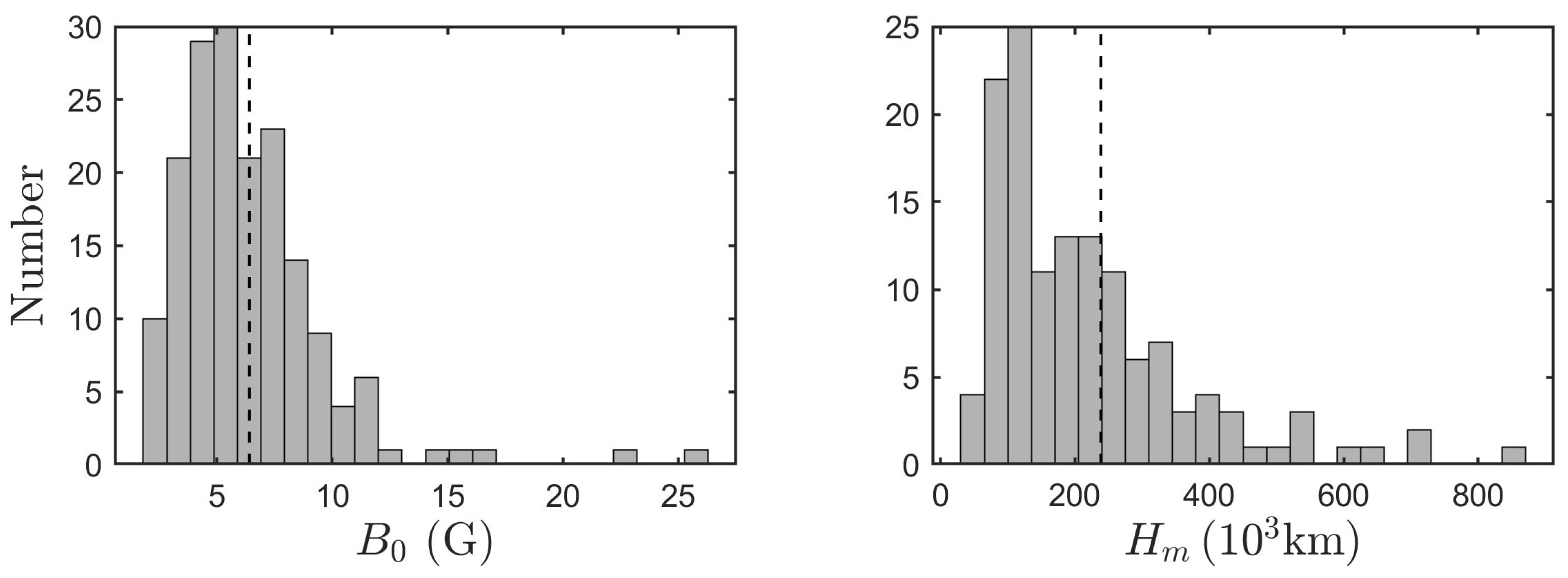
6.1.3. Computation of the Exciter Speed and the Magnetic Field

The observational data can be used to estimate the characteristic parameters of the fiber bursts, such as the exciter speed, $v_{exc}$, and the ambient magnetic field, B; the magnetic field value leads to the identification of the emission process. We start this section with the description of a simple computation, and then we precede to more sophisticated ones.

In the simplest case, the exciter speed, $v_{exc}$, can be computed from the fiber frequency drift rate, $\left(\frac{df}{fdt}\right)$, under the assumption of a coronal density model, which will provide the frequency scale height, $H_f$ (see Equations (1) and (2) in Section 2.2.3). In our computations [57], we used the hydrostatic model of Equation (2) with a coronal temperature $T=2.0\times {10}^{6}K$ and a four fold Newkirk coronal density model. The histogram of the exciter speed is shown in the left panel of Figure 24.

From the exciter speed, the magnetic field can be calculated under the assumption that the fiber exciter is either a whistler or an Alfvén wave, as outlined below; from the comparison of the value of B with independent estimates, the type of the exciter can be deduced.

In the case of whistler–Langmuir wave interaction we set the exciter speed equal to the whistler group speed, $v_{exc}=v_w$ and, following Kuijpers [83], we have

$$v_w=2c\left(\frac{{\omega }_{ce}}{{\omega }_p}\right)\sqrt{x{(1-x)}^3}=2c\left(\frac{f_w}{f}\right)\sqrt{\frac{{(1-x)}^3}{x}},$$

(7)

where

$$x=\frac{{\omega }_w}{{\omega }_{ce}}=\frac{f_w\left[\mathrm{MHz}\right]}{2.8B\left[\mathrm{G}\right]}$$

(8)

and the whistler frequency, $f_w$, is equal to the frequency difference between the absorption and emission peaks. Combining with Equation (1), we obtain for the drift rate:

$$\frac{df}{dt}=-2c{f}_w\frac{cos\varphi }{H_f}\sqrt{\frac{{(1-x)}^3}{x}}$$

(9)

which can be solved for x and hence for B. For propagation close to the radial, the $cos\varphi$ term can be ignored. In the case of Alfvén–Langmuir interaction [90], the exciter speed $v_{exc}$ is set equal to the Alfvén speed, $v_A$, from which the magnetic field can be directly computed.

In the middle and right panels of Figure 24, the magnetic fields in the case of whistler-driven and Alfvén-driven fibers are shown. In the first case, the average magnetic field was found to be $B=4.6\pm 1.5$ G and in the second $B=120\pm 50$ G.

Independent computations of the coronal magnetic field, B, (see the review by Alissandrakis and Gary [91]) are consistent with the value of B obtained under the assumption of whistler–Langmuir origin of the fiber exciter. Moreover, Bouratzis et al. [57] noted that the Alfvén emission mechanism requires an exceptionally cool and underdense loop for acceptable values of the coronal magnetic field.

We note that the above approach is model dependent, as a coronal density model is required. However, once the fiber emission process has been established, the characteristic parameters can be calculated independently of the density model. Bouratzis et al. [57] assumed constant scale height, $H_f/cos\varphi$, and a linear variation of x along the fiber, so that the drift rate in Equation (9) is expressed in terms of three parameters (scale height and the values of x at the start and at the end of the fiber), which can be determined from a least square fit. In one step further, (9) can be integrated to give an expression for the fiber track, $f\left(t\right)$, on the dynamic spectrum, again in terms of same three parameters.

In Figure 25, histograms of the values of the derived parameters, for the two computations mentioned above (fit of the drift rate for 38 outbound fiber groups and fit of the tracks for 209 individual fibers) are presented. The resulting histograms are quite similar. The average magnetic field was ≈4.44 G, very close to the results of the previous computation of the magnetic field at the beginning of this section. The minimum value of x computed from the fit was ≈0.29 and the maximum ≈0.6, consistent with the theoretical range of 0.25–0.5 in [83]. On the other hand, the range of x in individual fibers or groups was found to be ≲0.12, which is rather small. Therefore, the question regarding the exact conditions of the start and the end of the whistler–Langmuir wave interaction that gives rise to the electromagnetic emission almost suggests itself. Since the Landau and cyclotron damping in the case of whistler propagation at an angle (Section 3.3 [83]) is treated as negligible, it is possible that the range of x represents an upper bound. Furthermore, the effects of the dynamics of the energetic electrons trapped in the magnetic loop and the decrease of the loss-cone distribution with height might also result in a reduced range for x.

The average value of the deduced $H_f/cos\varphi$ was ∼220 Mm, comparable to the average model value of 250 Mm adopted in the previous computation of the ambient magnetic field. It is greater than the Newkirk frequency scale height (190–150 Mm), since it was calculated along the non-radial exciter trajectory.

Finally, Bouratzis et al. ([57], in their Section 5.2) employed a simple geometrical model of fiber propagation on a semi-circular coronal loop and a dipole magnetic field. From the frequency range of the fibers, their onset was found to be at an average height of 46 Mm, with an average vertical extent of 15 Mm. Then, from the scale height computed in the previous paragraphs, $cos\varphi$ and the semicircular loop radius were calculated; the latter was found to be ≈50–200 Mm, with few cases exceeding 250 Mm. Finally, the magnetic field (Figure 26) at the loop footpoints (16 G), the magnetic scale height (≈238 Mm on average), and the magnetic mirror ratio of the loop (≈1.9) were estimated. The value of the magnetic scale height and the rather small mirror ratio imply that the variation of the magnetic field with height is rather small. The results are consistent with previous calculations by [85,167] of the 3D path of a few select fibers along magnetic lines.

6.1.4. Relations between Observed Parameters

A number of empirical relations between measured parameters of fibers and the other members of the intermediate-drift bursts family are discussed below:

• Fiber repetition time, T, versus frequency drift rate, $\left|df/fdt\right|$: Based on the discussion in Kuijpers ([83], Section 4.2) and their measurements of fiber parameters, Bouratzis et al. ([57], Section 6.2) showed that, the $T\left|df/fdt\right|$ product, $\xi =0.0245\pm 0.0025$, is almost constant; they also provided a theoretical interpretation. The left panel of Figure 27 shows a scatter-plot of the the repetition time T, versus frequency drift rate bounded by the $\xi =0.0245\pm 0.0025$.
• Relative drift rate ($df/fdt$) versus relative instantaneous bandwidth ($\delta f/f$): Elgaroy and Soldal [168] were the first to obtain a linear relation between $df/fdt$ and $\delta f/f$ (see their Equation (2)). In ([57], Section 6.2) upper and lower bounds of the slope C of the linear equation were estimated; the results are shown in the middle panel panel of Figure 27.
• Repetition time, T, and duration at fixed frequency, $\delta t$: In ([57], Section 6.3) an empirical relationship $\delta t\approx 0.33T$ was presented and duly justified theoretically. The right panel of Figure 27 presents the scatter plot of measured duration at fixed frequency versus the repetition time, which is consistent with the linear relationship.

6.2. Spectral Imaging of Fibers

The question of the nature of the radiation process generating intermediate-drift bursts, fibers in particular, was addressed in Section 6.1.3. On the other hand, the relationship of the fibers to the type-IV burst background and the details of the fiber source structure are better studied with joint observations of images and dynamic spectra. To this end, two time intervals during the 14 July 2000 large solar event were selected for further study. This event was well covered by the SAO and ASG receivers and the three NRH frequencies (327.0 MHz, 410.5 MHz and 432.0 MHz) that fall within the SAO range. The intervals were 10:38:55–10:39:40 UT (Interval 1) and 11:00:05–11:00:50 UT (Interval 2) and contained fiber groups embedded in a broad-band continuum but no pulsations and other broad-band structures.

In our analysis of the data, the methods presented in Section 2.2 were used. These included computations of two-dimensional and one-dimensional NRH images and application of high-pass time filters to both the NRH images and the SAO dynamic spectra in order to enhance the fiber-associated emission. Low-pass filtering (30 s time integration) was used in the study of the background continuum.

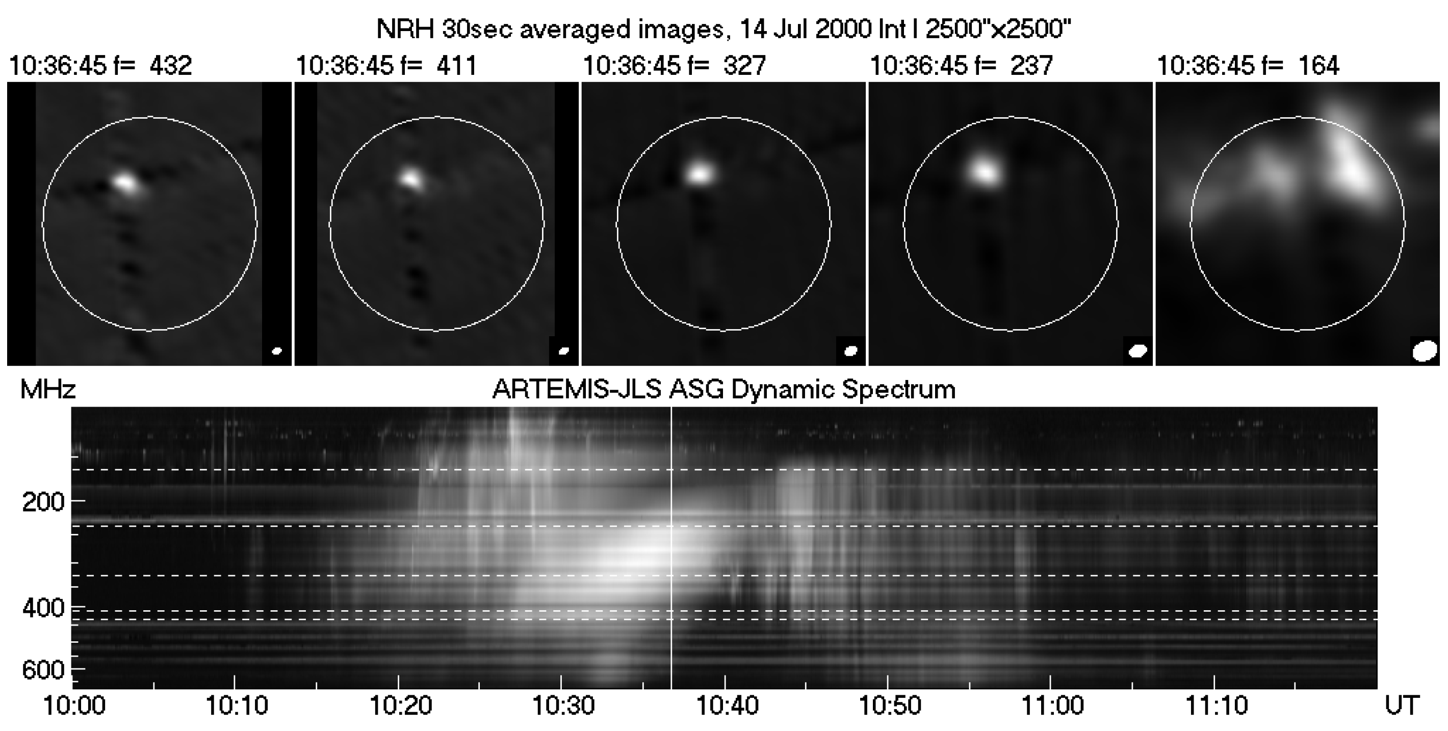
6.2.1. The Event of 14 July 2000—Evolution of the Type-IV Continuum

The event SOL2000-07-14T10:26:45, (see [169,170,171]) was quite complex. It originated in AR 9077 and was associated with an X5.7 extended flare (∼6${}^{\circ }$ E–8${}^{\circ }$ W, at ∼16${}^{\circ }$ N) starting at 10:03 UT and to a halo CME; an impressive loop system was recorded at 195 Å by TRACE (see Figure 1 of [172]). In [68,172], the evolution of the radio signatures of the event, jointly recorded by the ARTEMIS-IV/JLS and the NRH, were described; an outline of the associated fine structure is presented in Appendix A: Table 2 of [27].

A snapshot of the evolution of the continuum source, which provides the background to the fibers, is shown in the top panel of Figure 28 at the five NRH frequencies; the corresponding ASG dynamic spectrum is shown in the bottom panel of the same figure. The intensity of the embedded fibers represented a ∼10% rms fluctuation of the background. The full evolution of the background source is presented in [68], where a movie from 10:00 UT to 11:20 UT is given.

The details of the source displacement with time in the metric wavelengths are presented in [68,169,172]. In brief, at the onset of the event, the metric emission originated in the northwest, part of the solar disk, possibly associated with the primary energy release and the CME lift off. A new source northeast of the flare appeared at 10:27 UT (movie 1 of Alissandrakis et al. [68]), which dominated the drifting continuum. The first fibers were detected at 10:34 UT in this source. Soon after that, the continuum source drifted further to the northeast, at all frequencies except for 164 MHz until 10:39 UT. The motion of the continuum source could not be tracked after 10:40 UT, yet the development of multiple components and a net displacement to the southeast was detected, indicating a shift of the emission source lower in the corona. At 164 MHz, which was outside the drifting continuum, the emission did not follow the same evolution.

The above description indicates that the fibers first appeared in a moving type-IV source, which developed after the primary energy release. The fiber appearance was probably associated with the rapid expansion of the flare ribbons and the formation of post-flare loops in the eastern part of the flaring region. An association with the eastern footpoint of the CME flux rope is also possible.

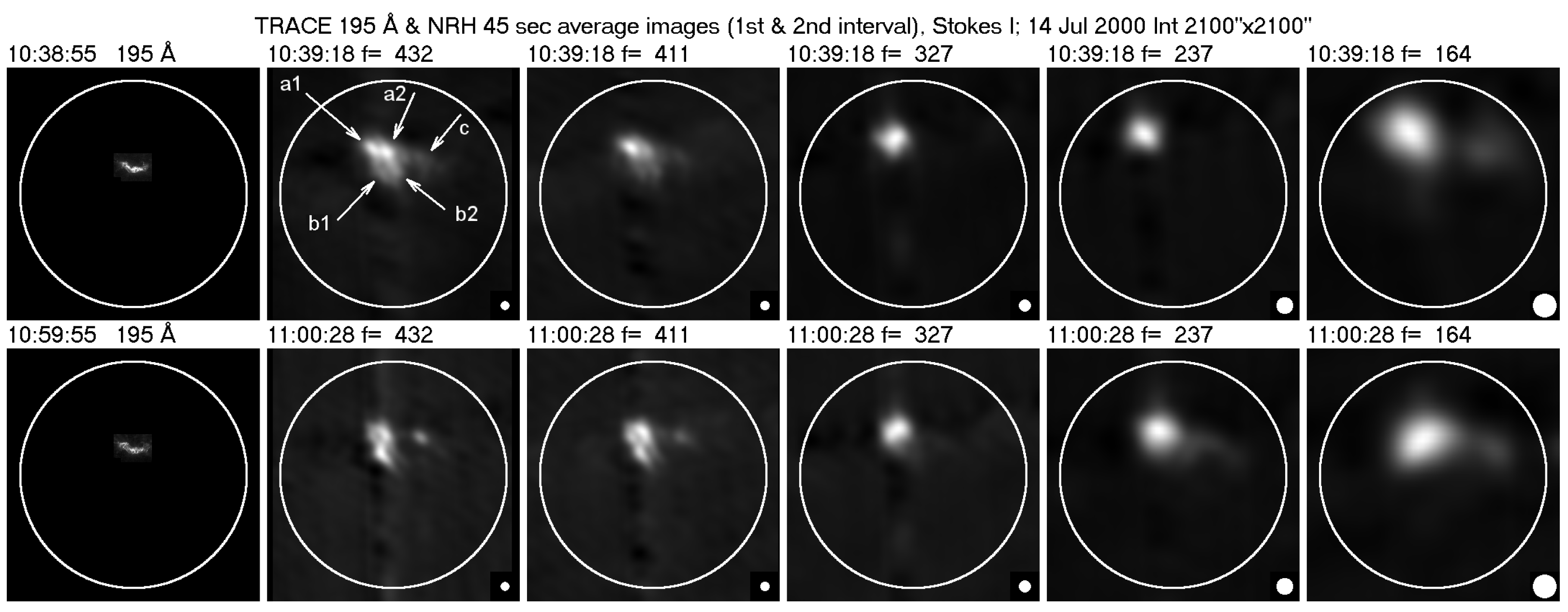
6.2.2. Structure of the Fiber-Emitting Sources

Before proceeding to the imaging of individual fibers, it is instructive to examine the overall structure of the fiber-emitting region. Average NRH images during Interval 1 (10:38:55–10:39:40 UT) and Interval 2 (11:00:05–11:00:50 UT) of spike activity are shown in Figure 29, together with the corresponding TRACE images at 195 Å. During the first interval the 432.0 and 327.0 MHz emission was dominated by two sources, marked a1 and a2 in the figure. These sources were located at the tip of two parallel, low-intensity stripes (b1 and b2 in the figure) extending to the southwest; there was also a weak source, c, in the west. Although there is considerable structural change between the two intervals, the same sources are detectable during the second interval.

All sources were strongly polarized, 50% or more, at all frequencies with the exception of 164 MHz in Interval 1. With the exception of source c during Interval 2, the polarization is in the right circular sense which, for o-mode emission, corresponds to magnetic polarity south of the neutral line. We note that the mere presence of fiber bursts indicates plasma emission and the strong polarization points to emission at the fundamental, which is expected to be highly polarized in the ordinary sense because the extraordinary mode is evanescent near this frequency.

The relative positions of the metric and EUV emissions are shown better in Figure 30. Here the EUV loop arcade serves in marking the neutral line of the magnetic field. In the same figure, we have plotted the positions of the stripes, measured on the 432.0 MHz image during the first interval (blue lines). The two stripes appear to define segments of large scale loops, with projected length of about 300 Mm. It is thus certain that the continuum source and the fibers were not associated with the 195 Å post-flare loops but with a much larger magnetic structure.

A possible explanation of the large size of the stripes compared to the EUV loops in terms of the flux rope flare/CME model is that they are segments of large-scale loops (red line in Figure 31) encompassing both the CME-associated flux rope and the EUV flare loops (blue line in the figure). The fact that we do not observe emission from the entire large scale loops could be attributed to the asymmetry of the magnetic field; in this case, it is possible that the instability will develop in one leg of the loop as, according to Aurass et al. [85], conditions for whistlers are more favorable at the weak field footpoint. The fact that all sources implicated in the fiber emission were polarized in the same sense supports the geometry suggested above.

6.2.3. Imaging of Individual Fibers

As noted previously, the most convenient way to visualize fine structures present in the NRH images is to compute 1D images (scans) and compare them with the dynamic spectrum, after application of time filtering [54]. Figure 32 shows the original and time-filtered 1D NRH intensity as a function of time for the second interval, with the 1D images computed in the NS direction; in the same figure we give the SAO dynamic spectrum (original, filtered in frequency and time, and filtered in time only), as well as the averaged NRH 2D images for reference. We note that, although fibers are hard to see in the original spectrum, they are readily visible in the filtered spectra. A similar improvement is noticed when comparing the time-filtered NRH 1D images to the original ones.

In spite of the lower time resolution of the NRH, practically all fiber bursts in the SAO spectra are detectable in the NRH 1D scans. They appear as short duration enhancements above the slowly varying background, rather than as discrete sources, which was the case with type-IV spikes (Section 4.2). Many fibers cross both the 432.0 and 410.5MHz frequency levels, but hardly any cross all three. Similar results were obtained for the first time interval.

6.2.4. Apparent Motions in Individual Fibers

In most cases, fibers in the 1D intensity–time displays (Figure 32) have the form of vertical streaks, which implies that the emission appears simultaneously over the entire structure. There are, however, cases where the fiber signatures are inclined, indicating apparent motions of individual features on the sky plane. One example is near 11:00:32 UT in the NS cuts of Figure 32. The inclinations suggest apparent motions from west to east and from south to north, i.e., from from the lower to the upper part of the loops associated with the two stripes. The apparent velocity, measured by 2d autocorrelation, is supra-luminal, ranging from 4c to 10c.

A different picture emerged from the examination of 2D images. In the left panel of Figure 33, we present 5-image (500 ms) long sequences of time filtered 2D images for four fibers at 432.0 MHz. The fiber around 11:00:05 UT (first row below the average image in the left panel) was practically stationary, while the other three showed clear apparent motions from southwest to northeast, in conformity with the results from the 1D image analysis. We first note that in some of the images shown in this figure, as well as in many others, fibers in absorption coexist with fibers in emission, both rapidly varying. Thus, what in the dynamic spectrum appears as a single fiber is actually a complex of multiple wave train that crosses the plasma level at slightly different times and positions, giving the impression of an apparent motion which may exhibit supra-luminal velocity. Figure 33 indicates that the duration of each train is comparable to the time difference between successive trains, which explains why such trains do not appear as separate fibers in the dynamic spectrum.

In the right panel of Figure 33, we give 5-image sequences at 432.0 MHz of the same fibers shown in the left panel. The comparison of fiber images at these closely spaced frequencies gave a time delay of 2.75 s for the first fiber and 1.5 s for the other three, corresponding to frequency drifts of $-7.8$ and $-14.3$ MHz s${}^{-1}$ respectively. Although the images of the same fiber at the two frequencies are similar, they are not identical. Differences could be attributed to the fact that the actual time delay is not an integer multiple of the image cadence, so that evolution effects play a role in the form of the radio sources.

6.2.5. Exciter Speed and Frequency Scale Length

During the second interval, we identified a pattern of fibers that varied smoothly between 432.0 MHz and 327.0 MHz. Using the method of cross correlation with a sliding spectral window, we computed the average track of this group of fibers on the dynamic spectrum, and from that we obtained time delays of 1.74 and 8.52 s for 410.5 MHz and 327.0 MHz, with respect to 432.0 MHz. We also measured the position shift in the average 2D images and we obtained shifts of 18${}^{″}$ and 58${}^{″}$ for 410.5 MHz and 327.0 MHz, with respect to 432.0 MHz. From these measurements, we computed the speed of the exciter on the plane of the sky and found a value of 5 Mm s${}^{-1}$, in good agreement with the computation from the frequency drift rate.

From the position shifts and the corresponding frequencies, we also computed the frequency scale length along the loop, projected on the plane of the sky, ${\ell }_f$ and obtained a value of ${\ell }_f=146$ Mm. On the other hand, the value of the frequency scale length along the loop, $h_f=H_f/cos\varphi$, where $H_f$ is the scale in the radial direction and $\varphi$ the angle between the loop segment and the vertical can be computed by fitting the average fiber track (see Section 6.1.3), assuming whistler origin of the emission. We obtained $h_f=183$ Mm. The comparison of ${\ell }_f$ and $h_f$ gave a value of $\varphi \sim 37$${}^{\circ }$, which places the fiber-emitting source above the middle of the leg of the large-scale loop.

Thus, the 2D images and the dynamic spectrum gave consistent results both for the exciter velocity and for the frequency scale length. In addition, spectral imaging provided an estimate of the angle between the loop segment and the vertical. Moreover, the analysis provided one more element in favor of whistler origin of fibers, since it was based on that assumption.

6.2.6. Fibers in Emission and Absorption

According to the theory of whistler origin (cf. Section 6.1.3), the fiber emission appears at $f_{pe}+f_w$ and the absorption at $f_{pe}$. Thus, at a fixed frequency, the absorption will precede the emission by $\Delta t=-f_w{(df/dt)}^{-1}$, where $df/dt$ is the frequency drift rate. The whistler frequency is equal to the frequency difference of the absorption and emission ridges, hence $\Delta t$ can be computed from the dynamic spectrum. It amounts to 350 ms for Interval 1 and 250 ms for Interval 2.

Figure 34 shows examples of fiber pairs in absorption and in emission; two pairs are presented for each frequency, all from Interval 1. The time difference is from 250 ms to 500 ms (2–4 NRH images), in conformity with the prediction of the previous paragraph. We note that the shape and size of the absorption and emission of each fiber pair are very similar, which verifies the hypothesis that they are manifestations of the same wave train.

7. Summary and Discussion

In this article, we have reviewed results of the study of fine structure associated with type-IV and -II solar radio bursts at metric wavelengths, based on radio spectra obtained by the SAO receiver of ARTEMIS-IV/JLS in the 270–450 MHz range at 128 frequency channels and some concurrent NRH imaging data. We focused on narrow-band bursts associated with type-IV continua and type-II shocks and on intermediate-drift bursts embedded in the type-IV continua. We note some inherent difficulties in the combined ARTEMIS/NRH studies, due to (a) the small number of common frequencies and (b) the lower time resolution of the NRH. In spite of these difficulties, fine structures were identified in both instruments, thus enriching our knowledge of their observable characteristics and providing improved insight into the emission mechanisms. In this section, we summarize the results presented in this review.

7.1. Classification of Fine-Structure Radio Bursts

Several, if not all, fine-structure classification efforts have been based on morphological criteria derived from dynamic spectra. The same approach has been adopted in the scheme proposed in [27] and presented in Section 3, which was based on observations in metric wavelengths. Compared with previous schemes, a novel two-level classification approach was adopted, which comprised a first level of five categories based on coarse spectral features and a second level with two or more subcategories based on the finer details of the features. This hierarchical arrangement provided some flexibility dictated by the diversity of the fine structures and a certain degree of compatibility with previous catalogs in the microwave–decimetric range (e.g., [23,24,26]). Furthermore, the five basic categories were statistically associated with the phases of the associated flare/CME evolution and the energy release process.

The inherent drawback of the above-mentioned classification method as well as most of its predecessors lies in the fact that they are based solely on morphology and not on the underlying physical and radiation processes. Thus certain subclasses, or even classes, may include bursts that are morphologically similar yet originate from different processes. There are several examples including, but not restricted to, narrow-band bursts (see Section 3.3), intermediate-drift bursts (Section 3.4), and emission bands (Section 3.5). Furthermore, the distinction between classes or subclasses is occasionally uncertain (see Section 3.5). However, despite these limitations, a classification scheme is necessary as a background for theoretical work (see, e.g., [16,174]).

7.2. Narrow-Band Burst (Spike) Source Structure

Our analysis of spikes (Section 4.1) in high time resolution dynamic spectra revealed their arrangement in various patterns, including spike chains in the form of N-bursts and lace-like bands, in addition to precise measurement and statistics of their observational characteristics. The analysis of simultaneous spectral and imaging data (Section 4.2) showed that spikes were located on top of a slowly varying background, provided by the type-IV continuum, at all frequencies. Most spikes were smaller than this background source, and many of them were displaced with respect to it, always remaining within its half width (see Figure 15 and Figure 16). This suggests that the spikes are additional emission, from small-scale reconnection within or very close to the continuum source, rather than fluctuations of the continuum background.

The data set of this report indicates that the spike brightness temperature of $T_B>2·{10}^8$ K precludes thermal emission and corroborates non-thermal or coherent emission mechanisms. Furthermore, the study of the dynamic spectra of spike chains provides evidence in favor of the plasma emission mechanism as it includes some chains of bi-directional spikes recorded in the 270–450 MHz range (see Figure 11 of Section 4.1), which appear to outline an X–reconnection front. A counter example was presented in [175,176], where multiple harmonics of spike groups in the 200–400 MHz range were reported.

The joint SAO and NRH observations of type-II–associated narrow-band spikes (Section 5.3) demonstrated that they constitute the predominant radio signature of the MHD shock. The comparison of characteristic parameters of type-II and type-IV spikes, such as their relative bandwidth and their duration, as well as their comparable brightness temperature, indicates that they are produced by similar emission processes.

We note that the spike chains which outline the shock front emission would appear as a continuous emission in dynamic spectra of lower resolution. It is therefore possible that, in low time-resolution spectra, quasi-parallel drifting spike chains might appear as multiple type-II lanes or “band-split of the band-split” as first reported by Magdalenić et al. [177].

7.3. Intermediate Drift Bursts (Fibers)

Our investigation of fiber bursts showed that this type of fine structure is by no means homogeneous but includes six morphological subclasses, which differ in the position of the emission and the absorption ridges (Section 3.4 and Section 6). The typical fibers with an emission ridge and a lower frequency absorption ridge comprise the dominant subclass, with the fibers of the remaining five subclasses being rare. Furthermore, a number of uncommon bursts of the intermediate-drift burst family, such as narrow-band fibers, rope-like fibers and fast-drift bursts have been recorded.

In addition to the classification and the statistics of the observational parameters of fibers (Section 6.1.2), we presented estimates of the magnetic field (Section 6.1.3). As mentioned previously, the fiber exciter could be the result of whistler–Langmuir interaction or of Alfvén–Langmuir interaction. Assuming a hydrostatic density model, we obtained from the observed drift rate a value of $B=4.6\pm 1.5G$ for whistler-driven fibers and $B=116\pm 50G$, for Alfvén-wave-driven fibers. The former value is close to estimates of B by other methods (e.g., [56,85,91,178,179]), thus suggesting the whistler mechanism as the most plausible. The Alfvén-wave-driven mechanism might be possible only within cool and underdense loops.

Having established the emission mechanism, the frequency drift rate and the track of a fiber on the dynamic spectrum can be computed. Furthermore, assuming a small, linear variation of the magnetic field along the path of the exciter, the magnetic field and its scale length along the exciter path can be computed by fitting the data, without resorting to a density model. This approach gave an average value of ∼4.4 G for the magnetic field and of ∼220 Mm for its scale along the exciter path.

The analysis of a spatially resolved type-IV continuum with embedded fiber-bursts employing SAO, NRH, and TRACE data gave additional important information:

In the NRH data the fibers did not appear as discrete sources but as short duration intensity modulations (approximately 10%) of the background continuum radio emission. (Section 6.2.1). We note that at decimetric wavelengths a modulation of about 30–40% has been reported (e.g., [56]).

The sources of the type-IV continuum and the embedded fibers were located on segments of large-scale loops, overlying the smaller EUV post flare loops (Section 6.2.2). We suggest that these large scale loops encompass both the CME-associated flux rope and the flare loops visible in EUV (Figure 31). The fact that the radiation was polarized in the same sense suggests further that the radio emission comes from one leg of these loops.

The appearance of multiple fibers in close succession and at slightly different positions on the radioheliograph images conveys the impression of apparent motion at supra-luminal velocities.

Direct measurement of the exciter speed in NRH images of fibers visible at two frequencies gave values consistent with the drift rate. Consistent results from spectral and imaging data were also obtained for the frequency scale length.

Finally, images of fiber pairs in absorption and in emission (Figure 34) showed that their shape and size were very similar; this verifies the hypothesis that they are manifestations of the same wave train.

8. Future Prospects and the New Generation of Spectroscopic Imaging Systems

The study of the radio-burst fine structure in the decimetric to decametric range is an open and promising field of research. Questions ranging from the plasma processes responsible for this type of radio emission to the association of the emission with active solar phenomena and different types of radiation (such as HXR) abound. The observational results obtained up to the present time have been subject to multiple interpretations for each type of FS. The future observational data of higher quality may lead to the resolution of the controversies related to the various theoretical models.

Results of particular interest have been obtained in the case of joint radioheliographic imaging and high resolution radio spectroscopy. However, a relatively limited set of observations have been available for this type of analysis. This is due to the lack of instruments capable of providing both spectral and imaging data, with the exception of LOFAR; thus, most spectral imaging has been performed with spectra and images from different instruments with different characteristics. The situation is improving; however, with a number of spectral imaging instruments in operation or under development (See also the review by [180]):

The Expanded Owens Valley Solar Array (EOVSA) [181,182] is a radio array dedicated to solar observations. It operates in the frequency range of 1–18 GHz and has a fast 20 ms sample time with a frequency resolution of approximately 50 MHz. EOVSA has the ability to measure and analyze the polarization properties of the solar radio signals in all four Stokes parameters (IQUV). The angular resolution of EOVSA varies depending on the observed frequency, ranging from 3.2${}^{″}$ to 57${}^{″}$.

SRH is a solar dedicated intereferometer, succeeding the Siberian Solar Radio Telescope (SSRT). Currently, it operates in the 3–12 GHz range, but when completed, it will cover the frequency range of 3–24 GHz with 10 MHz spectral, 0.1 s time and up to 7${}^{″}$ spatial resolution [183].

The RATAN-600 radio telescope is being equipped with a new receiver complex, capable of 122 kHz spectral and 8 ms time resolution in the 1–3 GHz range [184]. Although RATAN-600 is a transit instrument providing 1D solar images, it is expected to give interesting results if a burst occurs during the transit.

MUSER (Mingantu Ultrawide Spectral Radioheliograph, [185]) is a solar-dedicated radio telescope situated at the Mingantu Observing Station in China. With two arrays, MUSER-I and MUSER-II, it covers a frequency range from 400 MHz to 15 GHz. MUSER-I provides full-disk solar radio images in 64 frequency channels, with a time cadence of 25 ms and a spatial resolution of 51.6${}^{″}$ to 10.3${}^{″}$. MUSER-II records full-disk solar images in 520 channels, with a time cadence of 206.25 ms and a spatial resolution of 10.3${}^{″}$ to 1.3${}^{″}$. MUSER offers high temporal, spatial, and spectral resolutions, a dynamic range of 25 dB, and polarization capabilities. An extension of MUSER into the 30–400 MHz range is under way.

The Low-Frequency Array (LOFAR, [186,187]), though not a solar-dedicated instrument, provides extended capabilities in the radio observation of the Sun at the 10–240 MHz frequency range; furthermore, it is capable of radio spectroscopic imaging. The LOFAR high spatial, spectral, and temporal resolution characteristics vary with the selected observation mode as they are subject to the necessary design trade-offs. The angular resolution depends on frequency and baseline; at 1550 Km, the resolution is nominally 0.1${}^{″}$–3.2${}^{″}$ but the scattering of radio waves within the solar corona may limit it to ∼10${}^{″}$ [188]. In “tied-array” observation mode, for example, the time resolution is about 83 ms and the frequency resolution is 12.5 kHz [189,190]. On the other hand, with core and remote baselines (stations within the Netherlands) in solar observations, the highest achieved spatial resolution for LOFAR-LBA at 30 MHz was ∼80${}^{″}$, [191]. This was obtained using the longest baseline length of 48 km.

Finally, the Square Kilometer Array (SKA) will have solar observing capabilities [192]. The Murchison–Widefield Array (MWA), an SKA pathfinder, has already produced some interesting results (see, e.g., [193]).

The specifications of the next generation of instruments and the quality of the data need to be defined on the basis of the accumulated experience. Tan et al. [194] have compiled a number of recommendations as regards the constraints imposed by the narrow-band radio bursts, such as spikes, since they are the fine structures with the smallest frequency extend and the shortest duration. Thee recommendations, summarized below, may serve as guidelines for the design of new solar radio telescopes. They apply to the solar broadband radiospectrographs, solar radioheliographs, and to the imaging spectroscopy instruments capable of high time and frequency resolution multifrequency imaging [195]:

• The time and frequency resolution of a radiospectrograph should be consistent with the duration and the frequency extend of the smallest fine structure (e.g., spikes); in the case of radioheliographs, similar time resolution is highly desirable. The angular resolution should also be consistent with the bandwidth of the FS as the latter corresponds to its spatial extend. The duration and the frequency extent of the spikes depend on the observation frequency (see Section 5.3 and [148,149,150,151,194] for the applicable scaling laws) so that the corresponding resolution may be selected accordingly.
• At least two data points need be recorded per isolated spike burst. This corresponds to a sampling interval less than half of the averaged spike duration. Furthermore, the two data points are the minimum resolution required for spike frequency drift rate calculations. By the same argument, the frequency resolution should be less than half the averaged bandwidth.
• For radioheliographs, the same requirements as regards time and frequency resolution appear reasonable; however, the number of available frequency channels, the sensitivity requirement, and the computational power in the data processing pipeline may impose trade-offs (see [194]).
• The constraints presented above are applicable also to the members of the the inter- mediate-drift burst family; although the frequency extend of a considerable part of these exceeds significantly that of the spikes, their possible hyperfine structure of spike-like constituents should be considered.
• A combined radioheliograph-radiospectrograph capability with high time, frequency and angular resolution, as exemplified by the LOFAR, is highly desirable. The latter, depending on the observation frequency, is bound to require a rather large baseline.

References

1. Simnett, G.M.; Benz, A.O. The role of metric and decimetric radio emission in the understanding of solar flares. Astron. Astrophys. 1986, 165, 227–234. [Google Scholar]
2. Klein, K.L. Energetic electrons in impulsive solar flares: Radio diagnostics. Adv. Space Res. 2005, 35, 1759–1768. [Google Scholar] [CrossRef]
3. Huang, J.; Yan, Y.H.; Liu, Y.Y. A Study of Solar Radio Bursts with Fine Structures during Flare/CME Events. Sol. Phys. 2008, 253, 143–160. [Google Scholar] [CrossRef]
4. Morosan, D.E.; Kumari, A.; Kilpua, E.K.J.; Hamini, A. Moving solar radio bursts and their association with coronal mass ejections. Astron. Astrophys. 2021, 647, L12. [Google Scholar] [CrossRef]
5. Morosan, D.E.; Pomoell, J.; Kumari, A.; Vainio, R.; Kilpua, E.K.J. Shock-accelerated electrons during the fast expansion of a coronal mass ejection. Astron. Astrophys. 2022, 668, A15. [Google Scholar] [CrossRef]
6. Bárta, M.; Karlický, M. Radio Diagnostics of Solar Flare Reconnection. Hvar Obs. Bull. 2005, 29, 205–214. [Google Scholar]
7. Aurass, H. Signatures of magnetic reconnection in solar radio observations? Adv. Space Res. 2007, 39, 1407–1414. [Google Scholar] [CrossRef]
8. Pick, M. Overview of Solar Radio Physics and Interplanetary Disturbances. In Solar and Space Weather Radiophysics; Gary, D.E., Keller, C.U., Eds.; Astrophysics and Space Science Library Series; Springer: Berlin/Heidelberg, Germany, 2004; Volume 314, p. 17. [Google Scholar] [CrossRef]
9. Pick, M.; Vilmer, N. Sixty-five years of solar radioastronomy: Flares, coronal mass ejections and Sun Earth connection. Astron. Astrophys. Rev. 2008, 16, 1–153. [Google Scholar] [CrossRef]
10. Nindos, A.; Aurass, H.; Klein, K.L.; Trottet, G. Radio Emission of Flares and Coronal Mass Ejections. Invited Review. Sol. Phys. 2008, 253, 3–41. [Google Scholar] [CrossRef]
11. Kouloumvakos, A.; Nindos, A.; Valtonen, E.; Alissandrakis, C.E.; Malandraki, O.; Tsitsipis, P.; Kontogeorgos, A.; Moussas, X.; Hillaris, A. Properties of solar energetic particle events inferred from their associated radio emission. Astron. Astrophys. 2015, 580, A80. [Google Scholar] [CrossRef]
12. Kalaivani, P.P.; Prakash, O.; Shanmugaraju, A.; Feng, L.; Lu, L.; Gan, W.; Michalek, G. Analysis of Type II and Type III Radio Bursts Associated with SEPs from Non-Interacting/Interacting Radio-Loud CMEs. Astrophysics 2021, 64, 327–344. [Google Scholar] [CrossRef]
13. Kalaivani, P.P.; Shanmugaraju, A.; Prakash, O.; Kim, R.S. Statistical Characteristics on SEPs, Radio-Loud CMEs, Low Frequency Type II and Type III Radio Bursts Associated with Impulsive and Gradual Flares. Earth Moon Planets 2020, 123, 61–85. [Google Scholar] [CrossRef]
14. Miteva, R.; Samwel, S.W.; Zabunov, S. Solar Radio Bursts Associated with In Situ Detected Energetic Electrons in Solar Cycles 23 and 24. Universe 2022, 8, 275. [Google Scholar] [CrossRef]
15. Klein, K.L.; Musset, S.; Vilmer, N.; Briand, C.; Krucker, S.; Francesco Battaglia, A.; Dresing, N.; Palmroos, C.; Gary, D.E. The relativistic solar particle event on 28 October 2021: Evidence of particle acceleration within and escape from the solar corona. Astron. Astrophys. 2022, 663, A173. [Google Scholar] [CrossRef]
16. Benz, A.O. Radio Diagnostics of Flare Energy Release. In Energy Conversion and Particle Acceleration in the Solar Corona; Lecture Notes in Physics Series; Klein, L., Ed.; Springer: Berlin, Germany, 2003; Volume 612, pp. 80–95. [Google Scholar] [CrossRef]
17. Nindos, A.; Aurass, H. Pulsating Solar Radio Emission. In The High Energy Solar Corona: Waves, Eruptions, Particles; Lecture Notes in Physics Series; Klein, K.-L., MacKinnon, A.L., Eds.; Springer: Berlin, Germany, 2007; Volume 725, pp. 251–277. [Google Scholar] [CrossRef]
18. Bernold, T. A catalogue of fine structures in type IV solar radio bursts. Astron. Astrophys. Suppl. Ser. 1980, 42, 43–58. [Google Scholar]
19. Slottje, C. Atlas of Fine Structures of Dynamic Spectra of Solar Type IV-dm and Some Type II Radio Bursts. Ph.D. Dissertation, Utrecht Observatory, Utrecht, The Netherlands, 1981. [Google Scholar]
20. Guedel, M.; Benz, A.O. A catalogue of decimetric solar flare radio emission. Astron. Astrophys. Suppl. Ser. 1988, 75, 243–259. [Google Scholar]
21. Isliker, H.; Benz, A.O. Catalogue of 1–3 GHz solar flare radio emission. Astron. Astrophys. Suppl. Ser. 1994, 104, 145–160. [Google Scholar]
22. Allaart, M.A.F.; van Nieuwkoop, J.; Slottje, C.; Sondaar, L.H. Fine structure in solar microwave bursts. Sol. Phys. 1990, 130, 183–199. [Google Scholar] [CrossRef]
23. Jiřička, K.; Karlický, M.; Mészárosová, H.; Snížek, V. Global statistics of 0.8–2.0 GHz radio bursts and fine structures observed during 1992-2000 by the Ondřejov radiospectrograph. Astron. Astrophys. 2001, 375, 243–250. [Google Scholar] [CrossRef]
24. Jiřička, K.; Karlický, M.; Mészárosová, H. Occurrences of different types of 0.8–2.0 GHz solar radio bursts and fine structures during the solar cycle. In Proceedings of the Second Solar Cycle and Space Weather Euroconference, Solspa 2001, Vico Equense, Italy, 24–29 September 2001; Sawaya-Lacoste, H., Ed.; ESA Special Publication: Paris, France, 2001; Volume 477, pp. 351–354. [Google Scholar]
25. Fu, Q.J.; Yan, Y.H.; Liu, Y.Y.; Wang, M.; Wang, S.J. A New Catalogue of Fine Structures Superimposed on Solar Microwave Bursts. Chin. J. Astron. Astrophys. 2004, 4, 176–188. [Google Scholar] [CrossRef]
26. Mészárosová, H.; Karlický, M.; Jiřička, K. Ten Types of Solar Radio Bursts and Fine Structures Observed by the Ondřejov 0.8–2.0 GHz Radio-Spectrograph. Hvar Obs. Bull. 2005, 29, 309–318. [Google Scholar]
27. Bouratzis, C.; Hillaris, A.; Alissandrakis, C.E.; Preka-Papadema, P.; Moussas, X.; Caroubalos, C.; Tsitsipis, P.; Kontogeorgos, A. Fine Structure of Metric Type IV Radio Bursts Observed with the ARTEMIS-IV Radio-Spectrograph: Association with Flares and Coronal Mass Ejections. Sol. Phys. 2015, 290, 219–286. [Google Scholar] [CrossRef]
28. Caroubalos, C.; Maroulis, D.; Patavalis, N.; Bougeret, J.L.; Dumas, G.; Perche, C.; Alissandrakis, C.; Hillaris, A.; Moussas, X.; Preka-Papadema, P.; et al. The New Multichannel Radiospectrograph ARTEMIS-IV/HECATE, of the University of Athens. Exp. Astron. 2001, 11, 23–32. [Google Scholar] [CrossRef]
29. Caroubalos, C.; Alissandrakis, C.E.; Hillaris, A.; Preka-Papadema, P.; Polygiannakis, J.; Moussas, X.; Tsitsipis, P.; Kontogeorgos, A.; Petoussis, V.; Bouratzis, C.; et al. Ten Years of the Solar Radiospectrograph ARTEMIS-IV. In Recent Advances in Astronomy and Astrophysics, Proceedings of the 7th International Conference of the Hellenic Astronomical Society, Lixourion, Greece, 8–11 September 2005; Conference Series; Solomos, N., Ed.; AIP: College Park, MD, USA, 2006; Volume 848, pp. 864–873. [Google Scholar] [CrossRef]
30. Kontogeorgos, A.; Tsitsipis, P.; Moussas, X.; Preka-Papadema, G.; Hillaris, A.; Caroubalos, C.; Alissandrakis, C.; Bougeret, J.L.; Dumas, G. Observing the Sun at 20–650 MHz at Thermopylae with Artemis. Space Sci. Rev. 2006, 122, 169–179. [Google Scholar] [CrossRef]
31. Kontogeorgos, A.; Tsitsipis, P.; Caroubalos, C.; Moussas, X.; Preka-Papadema, P.; Hilaris, A.; Petoussis, V.; Bouratzis, C.; Bougeret, J.L.; Alissandrakis, C.E.; et al. The improved ARTEMIS IV multichannel solar radio spectrograph of the University of Athens. Exp. Astron. 2006, 21, 41–55. [Google Scholar] [CrossRef]
32. Kontogeorgos, A.; Tsitsipis, P.; Caroubalos, C.; Moussas, X.; Preka-Papadema, P.; Hilaris, A.; Petoussis, V.; Bougeret, J.L.; Alissandrakis, C.E.; Dumas, G. Measuring solar radio bursts in 20–650 MHz. Measurement 2008, 41, 251–258. [Google Scholar] [CrossRef]
33. Kerdraon, A.; Delouis, J.M. The Nançay Radioheliograph. In Coronal Physics from Radio and Space Observations, Proceedings of the CESRA Workshop, Nouan le Fuzelier, France, 3–7 June 1996; Lecture Notes in Physics; Trottet, G., Ed.; Springer: Berlin, Germany, 1997; Volume 483, pp. 192–201. [Google Scholar] [CrossRef]
34. Klein, K.L.; Kerdraon, A. Solar physics at Nançay radio observatory: Recent developments. In Proceedings of the 2011 XXXth URSI General Assembly and Scientific Symposium, Istanbul, Turkey, 13–20 August 2011; IEEE: Piscataway, NJ, USA. [Google Scholar] [CrossRef]
35. Vasanth, V.; Chen, Y.; Feng, S.; Ma, S.; Du, G.; Song, H.; Kong, X.; Wang, B. An Eruptive Hot-channel Structure Observed at Metric Wavelength as a Moving Type-IV Solar Radio Burst. Astrophys. J. Lett. 2016, 830, L2. [Google Scholar] [CrossRef]
36. Vasanth, V.; Chen, Y.; Lv, M.; Ning, H.; Li, C.; Feng, S.; Wu, Z.; Du, G. Source Imaging of a Moving Type IV Solar Radio Burst and Its Role in Tracking Coronal Mass Ejection from the Inner to the Outer Corona. Astrophys. J. 2019, 870, 30. [Google Scholar] [CrossRef]
37. Alissandrakis, C.E.; Nindos, A.; Patsourakos, S.; Hillaris, A. Multiwavelength observations of a metric type II event. Astron. Astrophys. 2021, 654, A112. [Google Scholar] [CrossRef]
38. Alissandrakis, C.E.; Patsourakos, S.; Nindos, A.; Bouratzis, C.; Hillaris, A. First detection of metric emission from a solar surge. Astron. Astrophys. 2022, 662, A14. [Google Scholar] [CrossRef]
39. Brueckner, G.E.; Howard, R.A.; Koomen, M.J.; Korendyke, C.M.; Michels, D.J.; Moses, J.D.; Socker, D.G.; Dere, K.P.; Lamy, P.L.; Llebaria, A.; et al. The Large Angle Spectroscopic Coronagraph (LASCO). Sol. Phys. 1995, 162, 357–402. [Google Scholar] [CrossRef]
40. Yashiro, S.; Gopalswamy, N.; Michalek, G.; St. Cyr, O.C.; Plunkett, S.P.; Rich, N.B.; Howard, R.A. A catalog of white light coronal mass ejections observed by the SOHO spacecraft. J. Geophys. Res. 2004, 109, 7105. [Google Scholar] [CrossRef]
41. Gopalswamy, N.; Yashiro, S.; Michalek, G.; Stenborg, G.; Vourlidas, A.; Freeland, S.; Howard, R. The SOHO/LASCO CME Catalog. Earth Moon Planets 2009, 104, 295–313. [Google Scholar] [CrossRef]
42. Yashiro, S.; Gopalswamy, N.; St. Cyr, O.C.; Lawrence, G.; Michalek, G.; Young, C.A.; Plunkett, S.P.; Howard, R.A. Development of SOHO/LASCO CME Catalog and Study of CME Trajectories. In AGU Spring Meeting Abstracts; American Geophysical Union: Washington, DC, USA, 2001; p. 31. [Google Scholar]
43. Handy, B.N.; Acton, L.W.; Kankelborg, C.C.; Wolfson, C.J.; Akin, D.J.; Bruner, M.E.; Caravalho, R.; Catura, R.C.; Chevalier, R.; Duncan, D.W.; et al. The transition region and coronal explorer. Sol. Phys. 1999, 187, 229–260. [Google Scholar] [CrossRef]
44. Kahler, S.W.; Kreplin, R.W. The NRL SOLRAD X-ray detectors: A summary of the observations and a comparison with the SMS/GOES detectors. Sol. Phys. 1991, 133, 371–384. [Google Scholar] [CrossRef]
45. Lemen, J.R.; Duncan, D.W.; Edwards, C.G.; Friedlaender, F.M.; Jurcevich, B.K.; Morrison, M.D.; Springer, L.A.; Stern, R.A.; Wuelser, J.P.; Bruner, M.E.; et al. The solar x-ray imager for GOES. In Proceedings of the Telescopes and Instrumentation for Solar Astrophysics, San Diego, CA, USA, 3–8 August 2003; Proc. SPIE. Fineschi, S., Gummin, M.A., Eds.; SPIE: Washington, DC, USA, 2003; Volume 5171, pp. 65–76. [Google Scholar] [CrossRef]
46. Delaboudinière, J.P.; Artzner, G.E.; Brunaud, J.; Gabriel, A.H.; Hochedez, J.F.; Millier, F.; Song, X.Y.; Au, B.; Dere, K.P.; Howard, R.A.; et al. EIT: Extreme-Ultraviolet Imaging Telescope for the SOHO Mission. Sol. Phys. 1995, 162, 291–312. [Google Scholar] [CrossRef]
47. Lin, R.P.; Hurford, G.J.; Madden, N.W.; Dennis, B.R.; Crannell, C.J.; Holman, G.D.; Ramaty, R.; von Rosenvinge, T.T.; Zehnder, A.; van Beek, H.F.; et al. High-Energy Solar Spectroscopic Imager (HESSI) Small Explorer mission for the next (2000) solar maximum. In Proceedings of the Missions to the Sun II, San Diego, CA, USA, 19–24 July 1998; Society of Photo-Optical Instrumentation Engineers (SPIE) Conference Series. Korendyke, C.M., Ed.; SPIE: Washington, DC, USA, 1998; Volume 3442, pp. 2–12. [Google Scholar] [CrossRef]
48. Lin, R.P.; Dennis, B.R.; Hurford, G.J.; Smith, D.M.; Zehnder, A.; Harvey, P.R.; Curtis, D.W.; Pankow, D.; Turin, P.; Bester, M.; et al. The Reuven Ramaty High-Energy Solar Spectroscopic Imager (RHESSI). Sol. Phys. 2002, 210, 3–32. [Google Scholar] [CrossRef]
49. Fárník, F.; Garcia, H.; Karlický, M. New Solar Broad-Band Hard X-Ray Spectrometer: First Results. Sol. Phys. 2001, 201, 357–372. [Google Scholar] [CrossRef]
50. Fishman, G.J.; Meegan, C.A.; Parnell, T.A.; Wilson, R.B. The Burst and Transient Source Experiment for the Gamma-Ray Observatory. In Proceedings of the Gamma Ray Transients and Related Astrophysical Phenomena, La Jolla, CA, USA, 5–8 August 1981; American Institute of Physics Conference Series. Lingenfelter, R.E., Hudson, H.S., Worrall, D.M., Eds.; AIP: College Park, MD, USA, 1982; Volume 77, pp. 443–451. [Google Scholar] [CrossRef]
51. Fishman, G.J.; Meegan, C.A.; Parnell, T.A.; Wilson, R.B.; Paciesas, W. BATSE/GRO observational capabilities. In Proceedings of the High Energy Transients in Astrophysics, Santa Cruz, CA, USA, 11–22 July 1983; American Institute of Physics Conference Series. Woosley, S.E., Ed.; AIP: College Park, MD, USA, 1983; Volume 115, pp. 651–664. [Google Scholar] [CrossRef]
52. Guidice, D.A.; Cliver, E.W.; Barron, W.R.; Kahler, S. The Air Force RSTN System. Bull. Am. Astron. Soc. 1981, 13, 553. [Google Scholar]
53. Messerotti, M.; Zlobec, P.; Padovan, S. The Trieste near-real-time coronal radio surveillance program: A tool for solar activity monitoring and forecasting. Mem. Soc. Astron. Ital. 2001, 72, 633–636. [Google Scholar]
54. Bouratzis, C.; Hillaris, A.; Alissandrakis, C.E.; Preka-Papadema, P.; Moussas, X.; Caroubalos, C.; Tsitsipis, P.; Kontogeorgos, A. High resolution observations with Artemis-IV and the NRH. I. Type IV associated narrow-band bursts. Astron. Astrophys. 2016, 586, A29. [Google Scholar] [CrossRef]
55. Armatas, S.; Bouratzis, C.; Hillaris, A.; Alissandrakis, C.E.; Preka-Papadema, P.; Kontogeorgos, A.; Tsitsipis, P.; Moussas, X. High-resolution observations with ARTEMIS/JLS and the NRH. IV. Imaging spectroscopy of spike-like structures near the front of type II bursts. Astron. Astrophys. 2022, 659, A198. [Google Scholar] [CrossRef]
56. Wang, Z.; Chen, B.; Gary, D.E. Dynamic Spectral Imaging of Decimetric Fiber Bursts in an Eruptive Solar Flare. Astrophys. J. 2017, 848, 77. [Google Scholar] [CrossRef]
57. Bouratzis, C.; Hillaris, A.; Alissandrakis, C.E.; Preka-Papadema, P.; Moussas, X.; Caroubalos, C.; Tsitsipis, P.; Kontogeorgos, A. High resolution observations with Artemis-JLS. II. Type IV associated intermediate drift bursts. Astron. Astrophys. 2019, 625, A58. [Google Scholar] [CrossRef]
58. Tsitsipis, P.; Kontogeorgos, A.; Moussas, X.; Preka-Papadema, P.; Hillaris, A.; Petoussis, V.; Caroubalos, C.; Alissandrakis, C.E.; Bougeret, J.L.; Dumas, G. Detection of slopes of linear and quasi-linear structures in noisy background, using 2D-FFT. In Recent Advances in Astronomy and Astrophysics, Proceedings of the 7th International Conference of the Hellenic Astronomical Society, Lixourion, Greece, 8–11 September 2005; American Institute of Physics Conference Series; Solomos, N., Ed.; AIP: College Park, MD, USA, 2006; Volume 848, pp. 874–882. [Google Scholar] [CrossRef]
59. Tsitsipis, P.; Kontogeorgos, A.; Hillaris, A.; Moussas, X.; Caroubalos, C.; Preka-Papadema, P. Fast estimation of slopes of linear and quasi-linear structures in noisy background, using Fourier methods. Pattern Recogn. 2007, 40, 563–577. [Google Scholar] [CrossRef]
60. Pohjolainen, S.; van Driel-Gesztelyi, L.; Culhane, J.L.; Manoharan, P.K.; Elliott, H.A. CME Propagation Characteristics from Radio Observations. Sol. Phys. 2007, 244, 167–188. [Google Scholar] [CrossRef]
61. Pohjolainen, S.; Hori, K.; Sakurai, T. Radio Bursts Associated with Flare and Ejecta in the 13 July 2004 Event. Sol. Phys. 2008, 253, 291–303. [Google Scholar] [CrossRef]
62. Armatas, S.; Bouratzis, C.; Hillaris, A.; Alissandrakis, C.E.; Preka-Papadema, P.; Moussas, X.; Mitsakou, E.; Tsitsipis, P.; Kontogeorgos, A. Detection of spike-like structures near the front of type II bursts. Astron. Astrophys. 2019, 624, A76. [Google Scholar] [CrossRef]
63. Newkirk, G.J. The Solar Corona in Active Regions and the Thermal Origin of the Slowly Varying Component of Solar Radio Radiation. Astrophys. J. 1961, 133, 983–1013. [Google Scholar] [CrossRef]
64. Vršnak, B.; Magdalenić, J.; Zlobec, P. Band-splitting of coronal and interplanetary type II bursts. III. Physical conditions in the upper corona and interplanetary space. Astron. Astrophys. 2004, 413, 753–763. [Google Scholar] [CrossRef]
65. Poquerusse, M. Relativistic type III solar radio bursts. Astron. Astrophys. 1994, 286, 611–625. [Google Scholar]
66. Klassen, A.; Karlický, M.; Mann, G. Superluminal apparent velocities of relativistic electron beams in the solar corona. Astron. Astrophys. 2003, 410, 307–314. [Google Scholar] [CrossRef]
67. Benz, A.O.; Monstein, C.; Beverland, M.; Meyer, H.; Stuber, B. High Spectral Resolution Observation of Decimetric Radio Spikes Emitted by Solar Flares—First Results of the Phoenix-3 Spectrometer. Sol. Phys. 2009, 260, 375–388. [Google Scholar] [CrossRef]
68. Alissandrakis, C.E.; Bouratzis, C.; Hillaris, A. High-resolution observations with ARTEMIS-JLS and the NRH. III. Spectroscopy and imaging of fiber bursts. Astron. Astrophys. 2019, 627, A133. [Google Scholar] [CrossRef]
69. Benz, A.O. Decimeter Burst Emission and Particle Acceleration. In Solar and Space Weather Radiophysics; Gary, D.E., Keller, C.U., Eds.; Astrophysics and Space Science Library Series; Springer: Berlin/Heidelberg, Germany, 2004; Volume 314, p. 203. [Google Scholar] [CrossRef]
70. Zhang, Y.; Tan, B.; Karlický, M.; Mészárosová, H.; Huang, J.; Tan, C.; Simões, P.J.A. Solar Radio Bursts with Spectral Fine Structures in Preflares. Astrophys. J. 2015, 799, 30. [Google Scholar] [CrossRef]
71. Huang, J.; Tan, B. Microwave Bursts with Fine Structures in the Decay Phase of a Solar Flare. Astrophys. J. 2012, 745, 186. [Google Scholar] [CrossRef]
72. Bouratzis, C.; Preka-Papadema, P.; Hillaris, A.; Tsitsipis, P.; Kontogeorgos, A.; Kurt, V.G.; Moussas, X. Radio Observations of the 20 January 2005 X-class Flare. Sol. Phys. 2010, 267, 343–359. [Google Scholar] [CrossRef]
73. Magdalenić, J.; Vršnak, B.; Zlobec, P.; Hillaris, A.; Messerotti, M. Classification and Properties of Supershort Solar Radio Bursts. Astrophys. J. Lett. 2006, 642, L77–L80. [Google Scholar] [CrossRef]
74. Magdalenić, J.; Hillaris, A.; Zlobec, P.; Vršnak, B. Millisecond solar radio bursts in the metric wavelength range. In Recent Advances in Astronomy and Astrophysics, Proceedings of the 7th International Conference of the Hellenic Astronomical Society, Lixourion, Greece, 8–11 September 2005; American Institute of Physics Conference Series; Solomos, N., Ed.; AIP: College Park, MD, USA, 2006; Volume 848, pp. 224–228. [Google Scholar] [CrossRef]
75. Tan, C.; Tan, B.; Yan, Y.; Wang, W.; Chen, L.; Liu, F.; Dou, Y. Fine structure events in microwave emission during solar minimum. Sol.-Terr. Phys. 2019, 5, 3–8. [Google Scholar] [CrossRef]
76. Tan, B.; Tan, C. Microwave Quasi-periodic Pulsation with Millisecond Bursts in a Solar Flare on 2011 August 9. Astrophys. J. 2012, 749, 28. [Google Scholar] [CrossRef]
77. Elgaroy, E.O. Solar Noise Storms; Pergamon Press: Oxford, UK, 1977; Volume 90, ISBN 0-08-021039-2. [Google Scholar]
78. Benz, A.O. Millisecond radio spikes. Sol. Phys. 1986, 104, 99–110. [Google Scholar] [CrossRef]
79. Benz, A.O. 4.1.2.8 Radio bursts of the non-thermal Sun. In Solar System, Landolt Börnstein- Group VI Astronomy and Astrophysics, Volume 4B; Springer: Berlin/Heidelberg, Germany, 2009; p. 189. [Google Scholar] [CrossRef]
80. Iwai, K.; Miyoshi, Y.; Masuda, S.; Tsuchiya, F.; Morioka, A.; Misawa, H. Spectral Structures and Their Generation Mechanisms for Solar Radio Type-I Bursts. Astrophys. J. 2014, 789, 4. [Google Scholar] [CrossRef]
81. Elgarøy, Ø. Intermediate drift bursts. In Proceedings of the CESRA-3, Committee of European Solar Radio Astronomers, Bordeaux, France, 21–22 September 1972; Delannoy, J., Poumeyrol, F., Eds.; Volume 3, p. 174. [Google Scholar]
82. Kuijpers, J. A possible generating mechanism for intermediate drift bursts. In Proceedings of the CESRA-3, Committee of European Solar Radio Astronomers, Bordeaux, France, 21–22 September 1972; Delannoy, J., Poumeyrol, F., Eds.; Volume 3, p. 130. [Google Scholar]
83. Kuijpers, J. Generation of intermediate drift bursts in solar type IV radio continua through coupling of whistlers and Langmuir waves. Sol. Phys. 1975, 44, 173–193. [Google Scholar] [CrossRef]
84. Kuijpers, J. Theory of type IV DM bursts. In Radio Physics of the Sun; Kundu, M.R., Gergely, T.E., Eds.; IAU Symposium; Springer: Berlin/Heidelberg, Germany, 1980; Volume 86, pp. 341–360. [Google Scholar]
85. Aurass, H.; Rausche, G.; Mann, G.; Hofmann, A. Fiber bursts as 3D coronal magnetic field probe in postflare loops. Astron. Astrophys. 2005, 435, 1137–1148. [Google Scholar] [CrossRef]
86. Mann, G.; Baumgaertel, K.; Chernov, G.P.; Karlicky, M. Interpretation of a special fine structure in type IV solar radio bursts. Sol. Phys. 1989, 120, 383–391. [Google Scholar] [CrossRef]
87. Chernov, G.P. Whistlers in the solar corona and their relevance to fine structures of type IV radio emission. Sol. Phys. 1990, 130, 75–82. [Google Scholar] [CrossRef]
88. Chernov, G.P. Solar Radio Bursts with Drifting Stripes in Emission and Absorption. Space Sci. Rev. 2006, 127, 195–326. [Google Scholar] [CrossRef]
89. Chernov, G.P. Unusual stripes in emission and absorption in solar radio bursts: Ropes of fibers in the meter wave band. Astron. Lett. 2008, 34, 486–499. [Google Scholar] [CrossRef]
90. Bernold, T.E.X.; Treumann, R.A. The fiber fine structure during solar type IV radio bursts - Observations and theory of radiation in presence of localized whistler turbulence. Astrophys. J. 1983, 264, 677–688. [Google Scholar] [CrossRef]
91. Alissandrakis, C.E.; Gary, D.E. Radio Measurements of the Magnetic field in the Solar Chromosphere and the Corona. Front. Astron. Space Sci. 2021, 7, 77. [Google Scholar] [CrossRef]
92. Tan, B. Diagnostic Functions of Solar Coronal Magnetic Fields from Radio Observations. Res. Astron. Astrophys. 2022, 22, 072001. [Google Scholar] [CrossRef]
93. Ni, S.; Chen, Y.; Li, C.; Zhang, Z.; Ning, H.; Kong, X.; Wang, B.; Hosseinpour, M. Plasma Emission Induced by Electron Cyclotron Maser Instability in Solar Plasmas with a Large Ratio of Plasma Frequency to Gyrofrequency. Astrophys. J. Lett. 2020, 891, L25. [Google Scholar] [CrossRef]
94. Ni, S.; Chen, Y.; Li, C.; Sun, J.; Ning, H.; Zhang, Z. An alternative form of the fundamental plasma emission through the coalescence of Z-mode waves with whistlers. Phys. Plasmas 2021, 28, 040701. [Google Scholar] [CrossRef]
95. Chernov, G.P. Manifestation of quasilinear diffusion on whistlers in the fine-structure radio sources of solar radio bursts. Plasma Phys. Rep. 2005, 31, 314–324. [Google Scholar] [CrossRef]
96. Zlotnik, E.Y.; Zaitsev, V.V.; Aurass, H.; Mann, G. A Special Radio Spectral Fine Structure Used for Plasma Diagnostics in Coronal Magnetic Traps. Sol. Phys. 2009, 255, 273. [Google Scholar] [CrossRef]
97. Zlotnik, E.Y.; Zaitsev, V.V.; Aurass, H.; Mann, G.; Hofmann, A. Solar type IV burst spectral fine structures. II. Source model. Astron. Astrophys. 2003, 410, 1011–1022. [Google Scholar] [CrossRef]
98. Aurass, H.; Klein, K.L.; Zlotnik, E.Y.; Zaitsev, V.V. Solar type IV burst spectral fine structures. I. Observations. Astron. Astrophys. 2003, 410, 1001–1010. [Google Scholar] [CrossRef]
99. Karlický, M.; Bárta, M.; Jiřička, K.; Mészárosová, H.; Sawant, H.S.; Fernandes, F.C.R.; Cecatto, J.R. Radio bursts with rapid frequency variations - Lace bursts. Astron. Astrophys. 2001, 375, 638–642. [Google Scholar] [CrossRef]
100. Fernandes, F.C.R.; Sawant, H.S.; Cecatto, J.R.; Krishan, V.; Karlický, M.; Rosa, R.R. Evidence of Plasma Resonance Instability from Observations of Solar Decimetric Fine Structures. Braz. J. Phys. 2003, 33, 109–114. [Google Scholar] [CrossRef]
101. Fernandes, F.C.R.; Krishan, V.; Andrade, M.C.; Cecatto, J.R.; Freitas, D.C.; Sawant, H.S. High resolution studies of intermediate drift bursts. Adv. Space Res. 2003, 32, 2545–2550. [Google Scholar] [CrossRef]
102. Chen, B.; Bastian, T.S.; Gary, D.E.; Jing, J. Spatially and Spectrally Resolved Observations of a Zebra Pattern in a Solar Decimetric Radio Burst. Astrophys. J. 2011, 736, 64. [Google Scholar] [CrossRef]
103. Chernov, G.P.; Markeev, A.K.; Poquerusse, M.; Bougeret, J.L.; Klein, K.L.; Mann, G.; Aurass, H.; Aschwanden, M.J. New features in type IV solar radio emission: Combined effects of plasma wave resonances and MHD waves. Astron. Astrophys. 1998, 334, 314–324. [Google Scholar]
104. Ning, Z.; Wu, H.; Xu, F.; Meng, X. High-Frequency Evolving Emission Lines for the 25 August 1999 Solar Flare. Sol. Phys. 2008, 250, 107–113. [Google Scholar] [CrossRef]
105. Xu, F.Y.; Yao, Q.J.; Meng, X.; Wu, H.A. Some Observed Results of Solar Radio Spectrometer at 4.5–7.5 GHz. Chin. J. Astron. Astrophys. 2001, 1, 469. [Google Scholar] [CrossRef]
106. Oberoi, D.; Evarts, E.R.; Rogers, A.E.E. High Temporal and Spectral Resolution Interferometric Observations of Unusual Solar Radio Bursts. Sol. Phys. 2009, 260, 389–400. [Google Scholar] [CrossRef]
107. Melrose, D.B.; Dulk, G.A. Electron-cyclotron masers as the source of certain solar and stellar radio bursts. Astrophys. J. 1982, 259, 844–858. [Google Scholar] [CrossRef]
108. Fleishman, G.D.; Mel’Nikov, V.F. Millisecond solar radio spikes. Sov. Phys. Uspekhi 1998, 41, 1157–1189. [Google Scholar] [CrossRef]
109. Chernov, G.P. Fine Structure of Solar Radio Bursts; Springer: Berlin/Heidelberg, Germany, 2011; Volume 375. [Google Scholar] [CrossRef]
110. Bakunin, L.M.; Chernov, G.P. Broadband Solar Bursts of the Spike Type. Sov. Astron. 1985, 29, 564–568. [Google Scholar]
111. Dabrowski, B.P.; Kus, A.J. Millisecond solar radio spikes observed at 1420 MHz. Mem. Soc. Astron. Ital. 2007, 78, 264. [Google Scholar]
112. Sawant, H.S.; Fernandes, F.C.R.; Cecatto, J.R.; Vats, H.O.; Neri, J.A.C.F.; Portezani, V.A.; Martinon, A.R.F.; Karlický, M.; Jiřička, K.; Mészárosová, H. Decimetric dot-like structures. Adv. Space Res. 2002, 29, 349–354. [Google Scholar] [CrossRef]
113. Caroubalos, C.; Poquerusse, M.; Bougeret, J.; Crepel, R. Radio evidence for a magnetic mirror effect on beams of subrelativistic electrons in the solar corona. Astrophys. J. 1987, 319, 503–513. [Google Scholar] [CrossRef]
114. Kuznetsov, A.A. On the superfine structure of solar microwave bursts. Astron. Lett. 2007, 33, 319–326. [Google Scholar] [CrossRef]
115. Chernov, G.P.; Sych, R.A.; Meshalkina, N.S.; Yan, Y.; Tan, C. Spectral and spatial observations of microwave spikes and zebra structure in the short radio burst of May 29, 2003. Astron. Astrophys. 2012, 538, A53. [Google Scholar] [CrossRef]
116. Tan, B.; Yan, Y.; Tan, C.; Sych, R.; Gao, G. Microwave Zebra Pattern Structures in the X2.2 Solar Flare on 2011 February 15. Astrophys. J. 2012, 744, 166. [Google Scholar] [CrossRef]
117. Bárta, M.; Karlický, M. Turbulent plasma model of the narrowband dm-spikes. Astron. Astrophys. 2001, 379, 1045–1051. [Google Scholar] [CrossRef]
118. Bárta, M.; Karlický, M. Radio Signatures of Solar Flare Reconnection. Astrophys. J. 2005, 631, 612–617. [Google Scholar] [CrossRef]
119. Bárta, M.; Büchner, J.; Karlický, M.; Skála, J. Spontaneous Current-layer Fragmentation and Cascading Reconnection in Solar Flares. I. Model and Analysis. Astrophys. J. 2011, 737, 24. [Google Scholar] [CrossRef]
120. Da̧browski, B.P.; Rudawy, P.; Falewicz, R.; Siarkowski, M.; Kus, A.J. Millisecond radio spikes in the decimetre band and their related active solar phenomena. Astron. Astrophys. 2005, 434, 1139–1153. [Google Scholar] [CrossRef]
121. Lantos, P.; Alissandrakis, C.E.; Rigaud, D. Quiet-Sun Emission and Local Sources at Meter and Decimeter Wavelengths and Their Relationship with the Coronal Neutral Sheet. Sol. Phys. 1992, 137, 225–256. [Google Scholar] [CrossRef]
122. Lantos, P. Low Frequency Observations of the Quiet Sun: A Review. In Proceedings of the Nobeyama Symposium, Kiyosato, Japan, 27–30 October 1998; Bastian, T.S., Gopalswamy, N., Shibasaki, K., Eds.; pp. 11–24. [Google Scholar]
123. Payne-Scott, R.; Yabsley, D.E.; Bolton, J.G. Relative Times of Arrival of Bursts of Solar Noise on Different Radio Frequencies. Nature 1947, 160, 256–257. [Google Scholar] [CrossRef]
124. Wild, J.P.; McCready, L.L. Observations of the Spectrum of High-Intensity Solar Radiation at Metre Wavelengths. I. The Apparatus and Spectral Types of Solar Burst Observed. Aust. J. Sci. Res. A Phys. Sci. 1950, 3, 387. [Google Scholar] [CrossRef]
125. Wild, J.P.; Smerd, S.F. Radio Bursts from the Solar Corona. Annu. Rev. Astron. Astrophys. 1972, 10, 159. [Google Scholar] [CrossRef]
126. Uchida, Y. On the Exciters of Type II and Type III Solar Radio Bursts. PPubl. ASJ 1960, 12, 376. [Google Scholar]
127. Aurass, H.; Mann, G. Radio Observation of Electron Acceleration at Solar Flare Reconnection Outflow Termination Shocks. Astrophys. J. 2004, 615, 526–530. [Google Scholar] [CrossRef]
128. Mann, G.; Warmuth, A.; Aurass, H. Generation of highly energetic electrons at reconnection outflow shocks during solar flares. Astron. Astrophys. 2009, 494, 669–675. [Google Scholar] [CrossRef]
129. Warmuth, A.; Mann, G.; Aurass, H. Modelling shock drift acceleration of electrons at the reconnection outflow termination shock in solar flares. Observational constraints and parametric study. Astron. Astrophys. 2009, 494, 677–691. [Google Scholar] [CrossRef]
130. Chrysaphi, N.; Reid, H.A.S.; Kontar, E.P. First Observation of a Type II Solar Radio Burst Transitioning between a Stationary and Drifting State. Astrophys. J. 2020, 893, 115. [Google Scholar] [CrossRef]
131. Smerd, S.F.; Sheridan, K.V.; Stewart, R.T. Split-band structure in type II radio bursts from the sun. Astrophys. Lett. 1975, 16, 23–28. [Google Scholar]
132. Du, G.; Chen, Y.; Lv, M.; Kong, X.; Feng, S.; Guo, F.; Li, G. Temporal Spectral Shift and Polarization of a Band-splitting Solar Type II Radio Burst. Astrophys. J. Lett. 2014, 793, L39. [Google Scholar] [CrossRef]
133. Du, G.; Kong, X.; Chen, Y.; Feng, S.; Wang, B.; Li, G. An Observational Revisit of Band-split Solar Type-II Radio Bursts. Astrophys. J. 2015, 812, 52. [Google Scholar] [CrossRef]
134. Ginzburg, V.L.; Zhelezniakov, V.V. On the mechanisms of sporadic solar radio emission. In Proceedings of the URSI Symp. 1: Paris Symposium on Radio Astronomy, Paris, France, 30 July–6 August 1958; IAU, Symposium. Bracewell, R.N., Ed.; Stanford University: Palo Alto, CA, USA, 1959; Volume 9, p. 574. [Google Scholar]
135. Gopalswamy, N. Recent advances in the long-wavelength radio physics of the Sun. Planet. Space Sci. 2004, 52, 1399–1413. [Google Scholar] [CrossRef]
136. Roberts, J.A. Solar Radio Bursts of Spectral Type II. Aust. J. Phys. 1959, 12, 327. [Google Scholar] [CrossRef]
137. Zaitsev, V.V.; Stepanov, A.V. Origin of electron streams generating the “herringbone” structure of type II bursts. Radiophys. Quantum Electron. 1974, 17, 936–943. [Google Scholar] [CrossRef]
138. Cairns, I.H.; Robinson, R.D. Herringbone bursts associated with type II solar radio emission. Sol. Phys. 1987, 111, 365–383. [Google Scholar] [CrossRef]
139. Vandas, M.; Karlický, M. On a Herringbone Structure of Solar Type II Bursts. In Magnetic Fields and Solar Processes, Proceedings of the 9th European Meeting on Solar Physics, Florence, Italy, 12–18 September, 1999; ESA Special Publication; Wilson, A., Ed.; ESA: Paris, France, 1999; Volume 448, p. 1071. [Google Scholar]
140. Carley, E.P.; Long, D.M.; Byrne, J.P.; Zucca, P.; Bloomfield, D.S.; McCauley, J.; Gallagher, P.T. Quasiperiodic acceleration of electrons by a plasmoid-driven shock in the solar atmosphere. Nat. Phys. 2013, 9, 811–816. [Google Scholar] [CrossRef]
141. Dorovskyy, V.V.; Melnik, V.N.; Konovalenko, A.A.; Brazhenko, A.I.; Panchenko, M.; Poedts, S.; Mykhaylov, V.A. Fine and Superfine Structure of the Decameter-Hectometer Type II Burst on 7 June 2011. Sol. Phys. 2015, 290, 2031–2042. [Google Scholar] [CrossRef]
142. Chernov, G.P. The relationship between fine structure of the solar radio emission at meter wavelengths and coronal transients. Astron. Lett. 1997, 23, 827–837. [Google Scholar]
143. Chernov, G.P.; Stanislavsky, A.A.; Konovalenko, A.A.; Abranin, E.P.; Dorovsky, V.V.; Rucker, G.O. Fine structure of decametric type II radio bursts. Astron. Lett. 2007, 33, 192–202. [Google Scholar] [CrossRef]
144. Chen, B.; Bastian, T.S.; Shen, C.; Gary, D.E.; Krucker, S.; Glesener, L. Particle acceleration by a solar flare termination shock. Science 2015, 350, 1238–1242. [Google Scholar] [CrossRef]
145. Fomichev, V.V.; Chernov, G.P. Solar Radio Bursts Associated with Standing Shock Waves. Geomagn. Aeron. 2020, 60, 137–150. [Google Scholar] [CrossRef]
146. Fomichev, V.; Chernov, G. Termination Shock as a Source of Unusual Solar Radio Bursts. Astrophys. J. 2020, 901, 65. [Google Scholar] [CrossRef]
147. Dauphin, C.; Vilmer, N.; Krucker, S. Observations of a soft X-ray rising loop associated with a type II burst and a coronal mass ejection in the 03 November 2003 X-ray flare. Astron. Astrophys. 2006, 455, 339–348. [Google Scholar] [CrossRef]
148. Guedel, M.; Benz, A.O. Time profiles of solar radio spikes. Astron. Astrophys. 1990, 231, 202–212. [Google Scholar]
149. Mészárosová, H.; Veronig, A.; Zlobec, P.; Karlický, M. Analysis of solar narrow band dm-spikes observed at 1420 and 2695 MHz. Astron. Astrophys. 2003, 407, 1115–1125. [Google Scholar] [CrossRef]
150. Rozhansky, I.V.; Fleishman, G.D.; Huang, G.L. Millisecond Microwave Spikes: Statistical Study and Application for Plasma Diagnostics. Astrophys. J. 2008, 681, 1688–1697. [Google Scholar] [CrossRef]
151. Csillaghy, A.; Benz, A.O. The bandwidth of millisecond radio spikes in solar flares. Astron. Astrophys. 1993, 274, 487. [Google Scholar]
152. Young, C.W.; Spencer, C.L.; Moreton, G.E.; Roberts, J.A. A Preliminary Study of the Dynamic Spectra of Solar Radio Bursts in the Frequency Range 500–950 Mc/s. Astrophys. J. 1961, 133, 243. [Google Scholar] [CrossRef]
153. Jiricka, K.; Karlický, M.; Mészárosová, H. High-frequency Intermediate Drift Bursts and Zebra Patterns. In Magnetic Fields and Solar Processes, Proceedings of the 9th European Meeting on Solar Physics, Florence, Italy, 12–18 September 1999; ESA Special Publication; Wilson, A., Ed.; ESA: Paris, France, 1999; Volume 448, p. 829. [Google Scholar]
154. Chernov, G.P. Some Features of the Formation of Filaments in Type IV Radio Bursts. Sov. Astron. 1990, 34, 66. [Google Scholar]
155. Kuijpers, J.; Slottje, C. Fiber bursts concurrent with a weak noise storm. Sol. Phys. 1976, 46, 247–252. [Google Scholar] [CrossRef]
156. Messmer, P.; Chernov, G.P.; Zlobec, P.; Gorgutsa, R. Unusual behaviour of zebra-pattern in the event July 28, 1999. In Solar Variability: From Core to Outer Frontiers, Proceedings of the 10th European Solar Physics Meeting, Prague, Czech Republic, 9–14 September 2002; ESA Special Publication; Wilson, A., Ed.; ESA: Paris, France, 2002; Volume 2, pp. 701–704. [Google Scholar]
157. Chernov, G.P.; Fomichev, V.V. Slowly drifting radio fibres. MNRAS 2023, 522, 1930–1938. [Google Scholar] [CrossRef]
158. Chernov, G.P.; Yan, Y.; Fu, Q.; Tan, C.; Wang, S. Unusual Zebra Patterns in the Decimeter Wave Band. Sol. Phys. 2008, 250, 115–131. [Google Scholar] [CrossRef]
159. Mann, G. Fiber bursts and related phenomena. Astron. Nachrichten 1990, 311, 409–412. [Google Scholar] [CrossRef]
160. Chernov, G.P. Behaviour of Whistlers in Coronal Magnetic Traps and its Relevance to a New Fine Structure in Solar Type–IV Radio Bursts. In Basic Plasma Processes on the Sun; IAU Symposium; Priest, E.R., Krishan, V., Eds.; Springer: Dordrecht, The Netherlands, 1990; Volume 142, p. 515. [Google Scholar]
161. Chernov, G.P.; Fomichev, V.V.; Gorgutsa, R.V.; Markeev, A.K.; Sobolev, D.E.; Hillaris, A.; Alissandrakis, K. Fine structural features of radio-frequency radiation of the solar flare of February 12, 2010. Geomagn. Aeron. 2014, 54, 406–415. [Google Scholar] [CrossRef]
162. Chernov, G. Chapter 5: Latest news on zebra patterns in the solar radio emission. In Solar Flares: Investigations and Selected Research; Nova Science Publishers, Inc.: Hauppauge, NY, USA, 2016; pp. 101–150. ISBN 978-1-53610-204-8. [Google Scholar]
163. Benz, A.O.; Mann, G. Intermediate drift bursts and the coronal magnetic field. Astron. Astrophys. 1998, 333, 1034–1042. [Google Scholar]
164. Nishimura, Y.; Ono, T.; Tsuchiya, F.; Misawa, H.; Kumamoto, A.; Katoh, Y.; Masuda, S.; Miyoshi, Y. Narrowband frequency-drift structures in solar type IV bursts. Earth Planets Space 2013, 65, 1555–1562. [Google Scholar] [CrossRef]
165. Melnik, V.N.; Konovalenko, A.A.; Brazhenko, A.I.; Rucker, H.O.; Dorovskyy, V.V.; Abranin, E.P.; Lecacheux, A.; Lonskaya, A.S. Bursts in emission and absorption as a fine structure of Type IV bursts. AIP Conf. Proc. 2010, 1206, 450–454. [Google Scholar] [CrossRef]
166. Slottje, C. Peculiar absorption and emission microstructures in the type IV solar radio outburst of March 2, 1970. Sol. Phys. 1972, 25, 210–231. [Google Scholar] [CrossRef]
167. Rausche, G.; Aurass, H.; Mann, G. Fiber Bursts and the Coronal Magnetic Field. Cent. Eur. Astrophys. Bull. 2008, 32, 43–50. [Google Scholar]
168. Elgaroy, O.; Soldal, O. Correlation between bandwidth and frequency drift velocity of intermediate drift bursts. Astron. Astrophys. 1981, 104, 99. [Google Scholar]
169. Klein, K.L.; Trottet, G.; Lantos, P.; Delaboudinière, J.P. Coronal electron acceleration and relativistic proton production during the 14 July 2000 flare and CME. Astron. Astrophys. 2001, 373, 1073–1082. [Google Scholar] [CrossRef]
170. Masuda, S.; Kosugi, T.; Hudson, H.S. A Hard X-ray Two-Ribbon Flare Observed with Yohkoh/HXT. Sol. Phys. 2001, 204, 55–67. [Google Scholar] [CrossRef]
171. Wang, S.; Yan, Y.; Zhao, R.; Fu, Q.; Tan, C.; Xu, L.; Wang, S.; Lin, H. Broadband Radio Bursts and Fine Structures during the Great Solar Event on 14 July 2000. Sol. Phys. 2001, 204, 153–164. [Google Scholar] [CrossRef]
172. Caroubalos, C.; Alissandrakis, C.E.; Hillaris, A.; Nindos, A.; Tsitsipis, P.; Moussas, X.; Bougeret, J.L.; Bouratzis, K.; Dumas, G.; Kanellakis, G.; et al. ARTEMIS IV Radio Observations of the 14 July 2000 Large Solar Event. Sol. Phys. 2001, 204, 165–177. [Google Scholar] [CrossRef]
173. Reeves, K.K.; Forbes, T.G. Predicted Light Curves for a Model of Solar Eruptions. Astrophys. J. 2005, 630, 1133–1147. [Google Scholar] [CrossRef]
174. Elgaroy, O. Discussion on the classification of fine structures in continua. Sol. Phys. 1986, 104, 41. [Google Scholar] [CrossRef]
175. Feng, S.W.; Chen, Y.; Li, C.Y.; Wang, B.; Wu, Z.; Kong, X.L.; Du, Q.F.; Zhang, J.R.; Zhao, G.Q. Harmonics of Solar Radio Spikes at Metric Wavelengths. Sol. Phys. 2018, 293, 39. [Google Scholar] [CrossRef]
176. Feng, S.W. The properties of solar radio spikes with harmonics and the associated EUV brightenings. Astrophys. Space Sci. 2019, 364, 4. [Google Scholar] [CrossRef]
177. Magdalenić, J.; Marqué, C.; Fallows, R.A.; Mann, G.; Vocks, C.; Zucca, P.; Dabrowski, B.P.; Krankowski, A.; Melnik, V. Fine Structure of a Solar Type II Radio Burst Observed by LOFAR. Astrophys. J. Lett. 2020, 897, L15. [Google Scholar] [CrossRef]
178. Rausche, G.; Aurass, H.; Mann, G.; Karlický, M.; Vocks, C. On Solar Intermediate Drift Radio Bursts at Decimeter and Meter Wavelength. Sol. Phys. 2007, 245, 327–343. [Google Scholar] [CrossRef]
179. Carley, E.P.; Vilmer, N.; Simões, P.J.A.; Ó Fearraigh, B. Estimation of a coronal mass ejection magnetic field strength using radio observations of gyrosynchrotron radiation. Astron. Astrophys. 2017, 608, A137. [Google Scholar] [CrossRef]
180. Gary, D.E. New Insights from Imaging Spectroscopy of Solar Radio Emission. Annu. Rev. Astron. Astrophys. 2023, 61. [Google Scholar] [CrossRef]
181. Gary, D.E.; Hurford, G.J.; Nita, G.M.; White, S.M.; McTiernan, J.; Fleishman, G.D. The Expanded Owens Valley Solar Array (EOVSA). In American Astronomical Society Meeting Abstracts #224; AAS: Washington, DC, USA, 2014; Volume 224, p. 123.60. [Google Scholar]
182. Gary, D.E. Early Observations with the Expanded Owens Valley Solar Array. In AAS/Solar Physics Division Abstracts #47; AAS: Washington, DC, USA, 2016; Volume 47, p. 301.01. [Google Scholar]
183. Altyntsev, A.; Lesovoi, S.; Globa, M.; Gubin, A.; Kochanov, A.; Grechnev, V.; Ivanov, E.; Kobets, V.; Meshalkina, N.; Muratov, A.; et al. Multiwave Siberian Radioheliograph. Sol.-Terr. Phys. 2020, 6, 30–40. [Google Scholar] [CrossRef]
184. Bogod, V.M.; Lebedev, M.K.; Ovchinnikova, N.E.; Ripak, A.M.; Storozhenko, A.A. Spectroradiometry of the Solar Corona on the RATAN-600. Cosm. Res. 2023, 61, 27–33. [Google Scholar] [CrossRef]
185. Yan, Y.; Chen, Z.; Wang, W.; Liu, F.; Geng, L.; Chen, L.; Tan, C.; Chen, X.; Su, C.; Tan, B. Mingantu Spectral Radioheliograph for Solar and Space Weather Studies. Front. Astron. Space Sci. 2021, 8, 20. [Google Scholar] [CrossRef]
186. de Vos, M.; Gunst, A.W.; Nijboer, R. The LOFAR Telescope: System Architecture and Signal Processing. IEEE Proc. 2009, 97, 1431–1437. [Google Scholar] [CrossRef]
187. van Haarlem, M.P.; Wise, M.W.; Gunst, A.W.; Heald, G.; McKean, J.P.; Hessels, J.W.T.; de Bruyn, A.G.; Nijboer, R.; Swinbank, J.; Fallows, R.; et al. LOFAR: The LOw-Frequency ARray. Astron. Astrophys. 2013, 556, A2. [Google Scholar] [CrossRef]
188. Dąbrowski, B.P.; Krankowski, A.; Rothkaehl, H.; Błaszkiewicz, L. Solar Studies with the LOFAR Telescope. In Proceedings of the 37th Meeting of the Polish Astronomical Society, Poznan, Poland, 7–10 September 2015; Różańska, A., Bejger, M., Eds.; The Polish Astronomical Society: Warszawa, Poland; Volume 3, pp. 116–119. [Google Scholar]
189. Morosan, D.E.; Gallagher, P.T.; Zucca, P.; Fallows, R.; Carley, E.P.; Mann, G.; Bisi, M.M.; Kerdraon, A.; Konovalenko, A.A.; MacKinnon, A.L.; et al. LOFAR tied-array imaging of Type III solar radio bursts. Astron. Astrophys. 2014, 568, A67. [Google Scholar] [CrossRef]
190. Carley, E.P.; Baldovin, C.; Benthem, P.; Bisi, M.M.; Fallows, R.A.; Gallagher, P.T.; Olberg, M.; Rothkaehl, H.; Vermeulen, R.; Vilmer, N.; et al. Radio observatories and instrumentation used in space weather science and operations. J. Space Weather Space Clim. 2020, 10, 7. [Google Scholar] [CrossRef]
191. Zhang, P.; Zucca, P.; Kozarev, K.; Carley, E.; Wang, C.; Franzen, T.; Dabrowski, B.; Krankowski, A.; Magdalenic, J.; Vocks, C. Imaging of the Quiet Sun in the Frequency Range of 20–80 MHz. Astrophys. J. 2022, 932, 17. [Google Scholar] [CrossRef]
192. Nindos, A.; Kontar, E.P.; Oberoi, D. Solar physics with the Square Kilometre Array. Adv. Space Res. 2019, 63, 1404–1424. [Google Scholar] [CrossRef]
193. Bhunia, S.; Carley, E.P.; Oberoi, D.; Gallagher, P.T. Imaging-spectroscopy of a band-split type II solar radio burst with the Murchison Widefield Array. Astron. Astrophys. 2023, 670, A169. [Google Scholar] [CrossRef]
194. Tan, B.l.; Cheng, J.; Tan, C.m.; Kou, H.x. Scaling-laws of Radio Spike Bursts and Their Constraints on New Solar Radio Telescopes. Chin. Astron. Astrophys. 2019, 43, 59–74. [Google Scholar] [CrossRef]
195. Bastian, T.S.; Gary, D.E.; White, S.M.; Hurford, G.J. Toward a Frequency-Agile Solar Radiotelescope. In Synoptic Solar Physics, Proceedings of the 18th NSO/Sacramento Peak Summer Workshop, Sunspot, NM, USA, 8–12 September 1997; Astronomical Society of the Pacific Conference Series; Balasubramaniam,, K.S., Harvey, J., Rabin, D., Eds.; ASP: Valencia, CA, USA, 1997; Volume 140, p. 563. [Google Scholar]
196. Lequeux, J.; Bertout, C.; Aghanim, N.; Forveille, T. Jean-Louis Steinberg (1922–2016). Astron. Astrophys. 2016, 586, E1. [Google Scholar] [CrossRef]
197. Da̧browski, B.P.; Rudawy, P.; Karlický, M. Millisecond Radio Spikes in the Decimetric Band. Sol. Phys. 2011, 273, 377–392. [Google Scholar] [CrossRef]
198. Melnik, V.N.; Shevchuk, N.V.; Konovalenko, A.A.; Rucker, H.O.; Dorovskyy, V.V.; Poedts, S.; Lecacheux, A. Solar Decameter Spikes. Sol. Phys. 2014, 289, 1701–1714. [Google Scholar] [CrossRef]
199. Shevchuk, N.V.; Melnik, V.N.; Poedts, S.; Dorovskyy, V.V.; Magdalenic, J.; Konovalenko, A.A.; Brazhenko, A.I.; Briand, C.; Frantsuzenko, A.V.; Rucker, H.O.; et al. The Storm of Decameter Spikes During the Event of 14 June 2012. Sol. Phys. 2016, 291, 211–228. [Google Scholar] [CrossRef]
200. Benz, A.O.; Csillaghy, A.; Aschwanden, M.J. Metric spikes and electron acceleration in the solar corona. Astron. Astrophys. 1996, 309, 291–300. [Google Scholar]
201. Messmer, P.; Benz, A.O. The Minimum bandwidth of narrowband spikes in solar flare decimetric radio waves. Astron. Astrophys. 2000, 354, 287–295. [Google Scholar]
202. Wang, M.; Xie, R.X. Millisecond spikes in a short decimetric solar radio burst. Sol. Phys. 1999, 185, 351–360. [Google Scholar] [CrossRef]
203. Chernov, G.P.; Fu, Q.J.; Lao, D.B.; Hanaoka, Y. Ion-Sound Model of Microwave Spikes with Fast Shocks in the Reconnection Region. Sol. Phys. 2001, 201, 153–180. [Google Scholar] [CrossRef]
204. Wang, S.J.; Yan, Y.H.; Liu, Y.Y.; Fu, Q.J.; Tan, B.L.; Zhang, Y. Solar Radio Spikes in 2.6–3.8 GHz during the 13 December 2006 Event. Sol. Phys. 2008, 253, 133–141. [Google Scholar] [CrossRef]
205. Benz, A.O.; Su, H.; Magun, A.; Stehling, W. Millisecond microwave spikes at 8 GHz during solar flares. Astron. Astrophys. Suppl. Ser. 1992, 93, 539–544. [Google Scholar]
Figure 1. An example of ARTEMIS-IV/JLS/SAO dynamic spectrum at 10 ms resolution, showing fiber bursts overlapping pulsating structure. (a) Original spectrum. (b) Differential spectrum (time derivative of flux). (c) After high-pass filtering along the time axis, which suppresses the continuum emission. (d) After an additional high-pass filter along the frequency axis, suppressing broad-band pulsation features. (e) Same as (c), after low-pass filtering along the frequency axis suppressing short time-scale features, fiber bursts in this case.
Universe 09 00442 g001
Figure 2. SAO dynamic spectrum of spikes during a six-second interval at full time resolution (10 ms). Dotted lines mark the frequencies of NRH data at 327.0, 410.5, and 432.0 MHz. The insert in the top right corner shows the autocorrelation function. (From [54] reproduced with permission).
Universe 09 00442 g002
Figure 3. Measurement of the width of temporal and frequency profiles of an individual spike within a cluster shown in the dynamic spectrum (a). Panel (b) shows the spectral profile and panel (c) the temporal profile. Panel (d) shows the full temporal profile at 340 MHz. (From [54], reproduced with permission).
Universe 09 00442 g003
Figure 4. Measurement of the duration and size of an individual spike in the NRH 1D (a) recording (same method as in Figure 3). Panel (b) shows the NRH total normalized flux in the east-west direction and panel (c) the temporal profile at 327 MHz. In panel (d), we present the ARTEMIS-JLS/SAO time profile at 327 MHz for comparison. The red curves in panels (b,c) trace the Gaussian fit used in the duration and width measurement of the spikes. The bright bands above and below the main one are due to sidelobes. (From [55] reproduced with permission).
Universe 09 00442 g004
Figure 5. (a) Tracking of individual fibers. (b) The same tracks are presented as a function of time from start. The red line corresponds to the average track reconstructed from integration of the drift rate measured using cross-correlation. (From [57], reproduced with permission).
Universe 09 00442 g005
Figure 6. (a): Original dynamic spectrum of a fiber group. (b) The same dynamic spectrum, filtered similarly to Figure 1c. (c): The two-dimensional autocorrelation function of the region delimited by the box in (b); the time lag in seconds is on the horizontal axis. (d,e) Profiles of the 2D autocorrelation function in the horizontal and the vertical direction, along the blue dashed lines in panel (c). (From [57], reproduced with permission).
Universe 09 00442 g006
Figure 7. Dynamic spectrum from SAO (a) for the fiber group (same group as in Figure 5) used in the computation of drift rate at a sliding frequency window using cross-correlation on each position of the window. Panels (b,c) show the frequency as a function of time shift from the first and last frequency window, labeled respectively with 1 and 2 in dynamic spectrum. Panel (d) shows the variation of the drift rate with frequency (From [57], reproduced with permission).
Universe 09 00442 g007
Figure 8. (a) Dynamic spectrum with two overlapping groups of intermediate-drift bursts. (b) Amplitude of the corresponding power spectrum as a function of the polar angle on the FT plane. (c) The same amplitude as a function of drift rate. The two peaks at 6 and 129 correspond to drift rates of 0.132 s 1 (fast drift burst) and −0.012 s 1 (typical fiber group), respectively (From [57], reproduced with permission).
Universe 09 00442 g008
Figure 9. (a) Histogram of spike duration; the line is an exponential fit. (b) Distribution of the relative instantaneous bandwidth of spikes. (Adapted from [54]).
Universe 09 00442 g009
Figure 10. Dynamic spectra of narrow-band bursts obtained by the ARTEMIS–JLS/SAO at high resolution (10 ms). (a) Broadband spike bursts. (b) Typical narrow-band structures. (From [54], reproduced with permission).
Universe 09 00442 g010
Figure 11. ARTEMIS/SAO high resolution (10 ms) dynamic spectra of drifting narrow-band structures. (Left): A group of bi-directional spikes. Above the line there are negative drifting spikes and below are positive drifting spikes. (Right): Spikes with positive and negative drifts. (From [54], reproduced with permission).
Universe 09 00442 g011
Figure 12. Dynamic spectra of U-like and J-like narrow-band bursts obtained by the ARTEMIS–JLS/SAO at high resolution. (From [54], reproduced with permission).
Universe 09 00442 g012
Figure 13. Spike chain recordings obtained by the ARTEMIS–JLS/SAO at high resolution (10 ms). The arrow points at a fiber that drifts almost parallel to the spike chain. (From [54], reproduced with permission).
Universe 09 00442 g013
Figure 14. Examples of peculiar spike group recordings obtained by the ARTEMIS–JLS/SAO at high resolution (10 ms): (Left): “Type III(N)” spike chain. (Right): Spike chain forming “lace-like” bands. (From [54], reproduced with permission).
Universe 09 00442 g014
Figure 15. (Top row):SAO dynamic spectrum. The position of the frequencies of the NRH are marked on the right. (Middle row): EW one-dimensional NRH images at 327 MHz as a function of time. (Bottom row): SAO time profiles at 327.1 and 325.6 MHz; the bar gives the intensity scale in arbitrary units. Adapted from [54].
Universe 09 00442 g015
Figure 16. Contour plots of 1D intensity vs. time after a high-pass filtering in time from the EW (left column) and the NS (right column) NRH arrays. The two lines along the time axis indicate the width of the background component (From [54], reproduced with permission).
Universe 09 00442 g016
Figure 17. Dynamic spectra of Event SOL2003-11-03T09:43:20 recorded by ARTEMIS-JLS. The top panel shows the full ASG spectrum with a time resolution of 1.5 s. In the middle panel, we show the SAO dynamic spectrum with a time resolution of 0.2 s and in the lower panel its time derivative, inside the 5 min box of the upper panel. The dashed horizontal lines mark three of the NRH frequencies. The boxes indicate selected segments of spike chains. (Adapted from [55]).
Universe 09 00442 g017
Figure 18. Panel (a) SAO dynamic spectrum for spike chain A (box in Figure 17). The corresponding frequency of the NRH is marked on the right. Panel (b) shows the NS 1D NRH images at 327 MHz. In Panel (c) we show the NRH (blue) and the SAO normalized total flux time profiles at 327 MHz and at 150 ms resolution (red) and 10 ms resolution (red dotted). Twelve spike-like structures are marked by vertical dashed lines. Panels (df): Same as in panels (ac) for the spike chain B at 410.5 MHz. Three spike-like structures are marked by vertical dashed lines (Adapted from [55]).
Universe 09 00442 g018
Figure 19. NRH images and SAO data at the beginning of the type-II emission at 327.0 MHz. Top: Sequence of NRH 2D images near the start of the type-II at 327 Mz. The color table of each image is normalized to the corresponding minimum and maximum intensity. The black arch marks the photosheric limb. Bottom: Flux as a function of time for NRH (blue) and for SAO (red). The time range of the images in the top row is marked by the double arrow (From [55], reproduced with permission).
Universe 09 00442 g019
Figure 20. Left: Source positions from 09:52:00 to 09:52:16 UT at 327.0 MHz and from 09:52:27 to 09:53:00 UT at 236.6 MHz, before (red) and during (black) the type-II. The black arch marks the photospheric limb. Middle: Brightness temperature, size, and position of sources as a function of time at 327.0 MHz. Right: Positions of the sources on the plane of the sky after 09:52:08 UT. Spike sources are marked as red asterisks in the middle and right panels (Adapted from [55]).
Universe 09 00442 g020
Figure 21. (a) Duration, δ τ , of narrow-band bursts and spikes versus frequency of observation, f; the dashed line is a plot of the empirical power law fit δ τ f 1.32 (b). Instantaneous bandwidth, δ f , in terms of the frequency of observation dependence of the same structures. The dashed line represents the empirical power law δ f 0.66 f 0.42 . ARTEMIS-IV/JLS results are color-coded in red and blue for type-IV and type-II bursts, respectively; the low frequency spikes are color-coded in black. The plotted data are from Table A1.
Universe 09 00442 g021
Figure 22. (Top Left): Isolated fiber with emission ridge only. (Top Right): Fibers appearing as absorption ridges on the type-IV continuum. (Bottom Left): Fibers with an emission ridge between two absorption ridges. (Bottom Right): Fibers with an absorption ridge between two emission ridges. All images are negative. Arrows point to emission ridges. Adapted from [57].
Universe 09 00442 g022
Figure 23. Typical fibers with an emission ridge and an LF absorption ridge. Adapted from [57].
Universe 09 00442 g023
Figure 24. Histograms of the exciter speed for 38 outbound typical fiber groups (left panel) and of the corresponding magnetic field assuming whistler (middle panel) and Alfvén waves (right panel) as exciters (From [57], reproduced with permission).
Universe 09 00442 g024
Figure 25. Histograms of fiber parameters derived from the least square fit of the drift rate of fiber groups (top) and the tracks of individual fibers (bottom). H f / cos ϕ is the frequency scale length along the exciter trajectory and B 1 , B 2 , the magnetic field at the start and at the end of the fibers (adapted from [57]).
Universe 09 00442 g025
Figure 26. Histograms of fiber parameters derived from a simple model dependent calculation; 209 individual fibers were used. Left: The magnetic field at the loop footpoints and Right: The magnetic scale height. The dashed vertical lines in each histogram mark the median of the respective data set (adapted from [57], Figure 20).
Universe 09 00442 g026
Figure 27. (Left): Fiber repetition time plotted against the relative drift rate. The blue lines represent the upper and lower bound of the dimensionless parameter, ξ (see text). Typical fibers are shown as red stars, rope-like fibers as blue triangles, and the FDBs as blue stars. (Middle): Relative drift rate ( d f / f d t ) versus relative instantaneous bandwidth ( δ f / f ). The data points are colour-coded as in the left panel; in addition, the fiber burst points from [152] (magenta diamond), [81] (blue and green diamond), and [90,166] (black diamond) are included in the same graph for comparison. The rope-like fibers from [89] are indicated with the black square. The dashed lines are the upper and lower bounds of the slope C = 0.8 s 1 and C = 8.0 s 1 . (Right Panel): Duration at fixed frequency ( δ t ) versus repetition time (T). The blue dashed line represents the linear relationship (see text). The data points are colour-coded as in the left panel (adapted from [57]).
Universe 09 00442 g027
Figure 28. (Top Panel): A sequence of 30 sec average NRH images in Stokes I at all five frequencies. The images have been normalized so that the minimum intensity of each image is black and the peak intensity is white. The white circles mark the photospheric limb. The NRH resolution (beam) is drawn in the lower right corner of each frame. The bottom panel shows the ARTEMIS-IV/JLS/ASG dynamic spectrum in the 100–670 MHz range, with the vertical white line marking the time of the images in the top panel and the dashed horizontal lines marking the NRH frequencies. (From [68], reproduced with permission).
Universe 09 00442 g028
Figure 29. Average NRH images in total intensity (Stokes I) during the first (top) and the second (bottom) interval, together with the corresponding TRACE images in the 195 Å band (left column). For the NRH images we used a circular clean beam in order to enhance some features. All images are normalized to their peak intensity. (From [68], reproduced with permission).
Universe 09 00442 g029
Figure 30. Contours of the average NRH images at 432 MHz during Interval 1 (left) and Interval 2 (right) superposed on top of the corresponding (negative) 195 Å TRACE images. The blue lines mark the position of the two stripes during the first interval. The red and green stars mark the position of the 327.0 and 237.0 MHz peaks, respectively. The NRH beam is plotted in the lower right corner (adapted from [68]).
Universe 09 00442 g030
Figure 31. Lines of force of the magnetic field, according to the model of Reeves and Forbes [173]. The blue line marks a flare loop and the red line a large scale loop. The flux rope and the current sheet are marked by the arrows. Positions are in arbitrary units.
Universe 09 00442 g031
Figure 32. (Left column): Original SAO dynamic spectrum and 1D Nançay NS images (scans) as a function of time for Interval 2. (Middle): The corresponding filtered images; in the top row the dynamic spectrum has been filtered in both time and frequency, in the others in time only. (Right): Average NRH images with the same orientation as the 1D images (north up). Dashed horizontal lines in the spectra mark the NRH frequencies. (From [68], reproduced with permission).
Universe 09 00442 g032
Figure 33. Time sequences of filtered NRH 2D images at 411 MHz (left) and 432 Mhz (right), showing the evolution of four fibers during the second interval. The time step is 125 ms. In the top row the corresponding average image is given for reference (Adapted from [68]).
Universe 09 00442 g033
Figure 34. Time−filtered images of fibers in absorption (top row) and in emission (bottom). One case is shown for each interval and each NRH frequency. Each pair of fiber images is normalized to the same minimum/maximum values. (From [68], reproduced with permission).
Universe 09 00442 g034