Gravitational Waves, μ Term and Leptogenesis from B − L Higgs Inflation in Supergravity

Abstract
1. Introduction
- (i)
- For , the observables depend on the ratio and can be done excellently consistent with the Planck [34] and Bicep2/Keck Array [35] results. More specifically, all data taken by the Bicep2/Keck Array CMB polarization experiments up to and including the 2014 observing season (BK14) [35] seem to favor r’s of order since the output of the analysis is
- (ii)
2. Model Description
2.1. Superpotential
- (a)
- is the part of W which contains the usual terms—except for the term—of MSSM, supplemented by Yukawa interactions among the left-handed leptons () and :Here the ith generation doublet left-handed quark and lepton superfields are denoted by and respectively, whereas the singlet antiquark [antilepton] superfields by and [ and ] respectively. The electroweak Higgs superfields which couple to the up [down] quark superfields are denoted by [].
- (b)
- is the part of W which is relevant for HI, the generation of the term of MSSM and the Majorana masses for ’s. It takes the form
2.2. Kähler Potential
3. Inflationary Scenario
3.1. Inflationary Potential
3.2. Stability and One-Loop Radiative Corrections
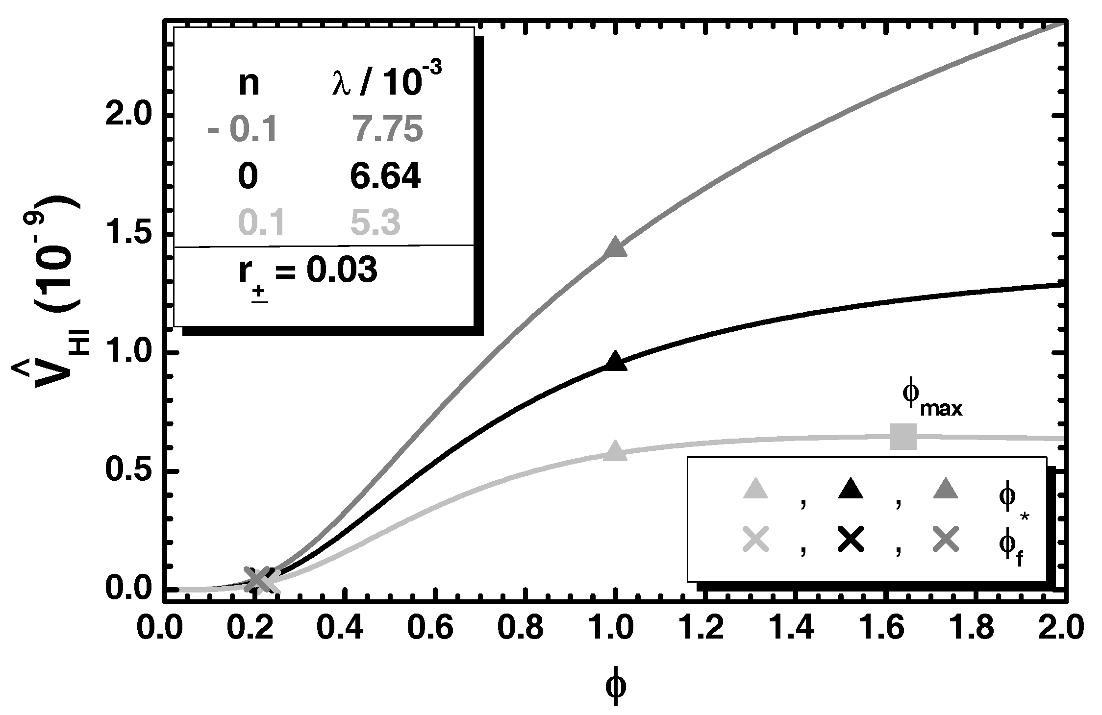
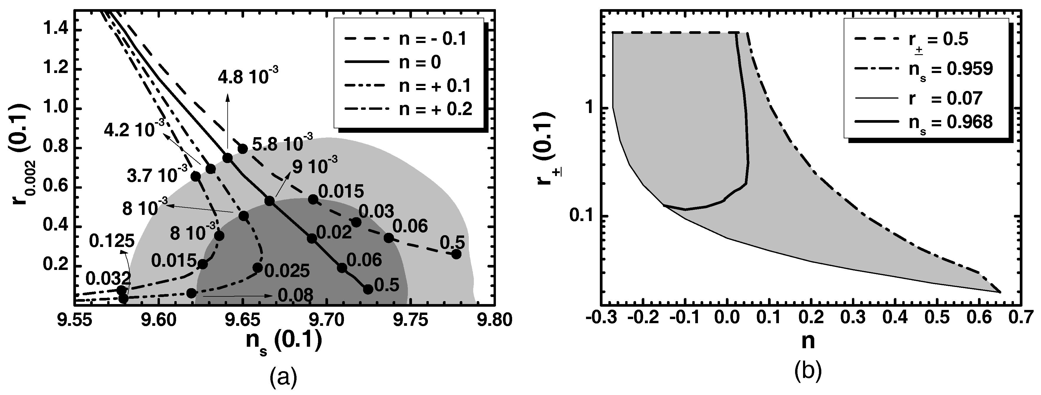
3.3. Inflationary Observables
3.4. Comparison with Observations
4. Higgs Inflation and μ Term of MSSM
4.1. SUSY Potential
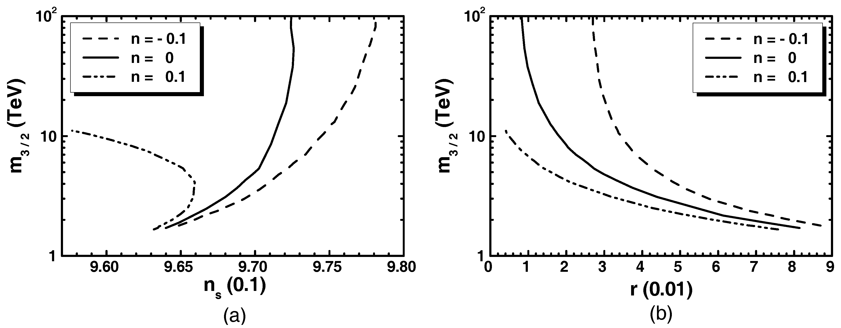
4.2. Generation of the μ Term of MSSM
4.3. Connection with the MSSM Phenomenology
5. Non-Thermal Leptogenesis and Neutrino Masses
5.1. Inflaton Mass and Decay
5.1.1. Mass Spectrum at the SUSY Vacuum
5.1.2. Inflaton Decay
5.2. Lepton-Number and Gravitino Abundances
5.3. Lepton-Number Asymmetry and Neutrino Masses
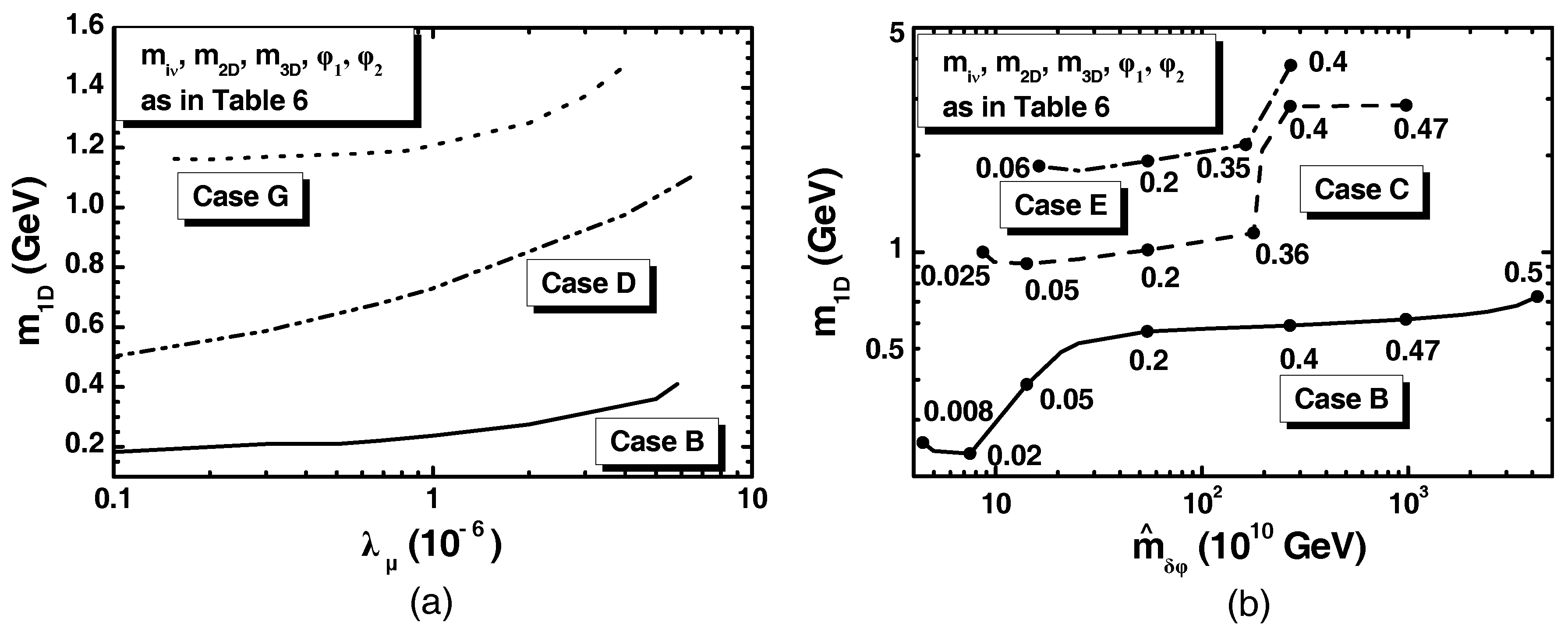
5.4. Results
6. Conclusions
Conflicts of Interest
References
- Guth, A.H. The Inflationary Universe: A Possible Solution to the Horizon and Flatness Problems. Phys. Rev. D 1981, 23, 347–356. [Google Scholar] [CrossRef]
- Linde, A.D. A New Inflationary Universe Scenario: A Possible Solution of the Horizon, Flatness, Homogeneity, Isotropy and Primordial Monopole Problems. Phys. Lett. B 1982, 108, 389–393. [Google Scholar] [CrossRef]
- Albrecht, A.; Steinhardt, P.J. Cosmology for Grand Unified Theories with Radiatively Induced Symmetry Breaking. Phys. Rev. Lett. 1982, 48, 1220–1223. [Google Scholar] [CrossRef]
- Salopek, D.S.; Bond, J.R.; Bardeen, J.M. Designing Density Fluctuation Spectra in Inflation. Phys. Rev. D 1989, 40, 1753–1788. [Google Scholar] [CrossRef]
- Cervantes-Cota, J.L.; Dehnen, H. Induced gravity inflation in the SU(5) GUT. Phys. Rev. D 1995, 51, 395–404. [Google Scholar] [CrossRef]
- Dvali, G.; Shafi, Q.; Schaefer, R. Large scale structure and supersymmetric inflation without fine tuning. Phys. Rev. Lett. 1994, 73, 1886–1889. [Google Scholar] [CrossRef] [PubMed]
- Covi, L.; Mangano, A.; Masiero, G.M. Hybrid inflation from supersymmetric SU(5). Phys. Lett. B 1998, 424, 253–258. [Google Scholar] [CrossRef]
- Kyae, B.; Shafi, Q. Inflation with realistic supersymmetric SO(10). Phys. Rev. D 2005, 72, 063515. [Google Scholar] [CrossRef]
- Kyae, B.; Shafi, Q. Flipped SU(5) predicts delta T/T. Phys. Lett. B 2006, 635, 247–252. [Google Scholar] [CrossRef]
- Jeannerot, R.; Khalil, S.; Lazarides, G. New shifted hybrid inflation. J. High Energy Phys. 2002, 2002, 069. [Google Scholar] [CrossRef]
- Buchmüller, W.; Domcke, V.; Schmitz, K. Spontaneous B-L Breaking as the Origin of the Hot Early Universe. Nucl. Phys. B 2012, 862, 587–632. [Google Scholar] [CrossRef]
- Pallis, C.; Toumbas, N. Non-Minimal Higgs Inflation and non-Thermal Leptogenesis in A Supersymmetric Pati-Salam Model. J. Cosmol. Astropart. Phys. 2011, 2011, 002. [Google Scholar] [CrossRef]
- Pallis, C.; Toumbas, N. Leptogenesis and Neutrino Masses in an Inflationary SUSY Pati-Salam Model. In Open Questions in Cosmology; Olmo, G.J., Ed.; InTech: Rijeka, Croatia, 2012; pp. 241–269. [Google Scholar]
- Antusch, S.; Bastero-Gil, M.; Baumann, J.P.; Dutta, K.; King, S.F.; Kostka, P.M. Gauge Non-Singlet Inflation in SUSY GUTs. J. High Energy Phys. 2010, 2010, 100. [Google Scholar] [CrossRef]
- Nakayama, K.; Takahashi, F. PeV-scale Supersymmetry from New Inflation. J. Cosmol. Astropart. Phys. 2012, 2012, 035. [Google Scholar] [CrossRef]
- Einhorn, M.B.; Jones, D.R.T. GUT Scalar Potentials for Higgs Inflation. J. Cosmol. Astropart. Phys. 2012, 2012, 049. [Google Scholar] [CrossRef]
- Heurtier, L.; Khalil, S.; Moursy, A. Single Field Inflation in Supergravity with a U(1) Gauge Symmetry. J. Cosmol. Astropart. Phys. 2015, 2015, 045. [Google Scholar] [CrossRef]
- Leontaris, G.K.; Okada, N.; Shafi, Q. Non-minimal quartic inflation in supersymmetric SO(10). Phys. Lett. B 2017, 2017, 256–259. [Google Scholar] [CrossRef]
- Arai, M.; Kawai, S.; Okada, N. Higgs inflation in minimal supersymmetric SU(5) grand unified theory. Phys. Rev. D 2011, 84, 123515. [Google Scholar] [CrossRef]
- Ellis, J.; He, H.J.; Xianyu, Z.Z. New Higgs Inflation in a No-Scale Supersymmetric SU(5) GUT. Phys. Rev. D 2015, 91, 021302. [Google Scholar] [CrossRef]
- Ellis, J.; He, H.J.; Xianyu, Z.Z. Higgs Inflation, Reheating and Gravitino Production in No-Scale Supersymmetric GUTs. J. Cosmol. Astropart. Phys. 2016, 2016, 068. [Google Scholar] [CrossRef]
- Kawai, S.; Kim, J. Multifield dynamics of supersymmetric Higgs inflation in SU(5) GUT. Phys. Rev. D 2016, 2016, 065023. [Google Scholar] [CrossRef]
- Ellis, J.; Garcia, M.A.G.; Nagata, N.; Nanopoulos, D.V.; Olive, K.A. Starobinsky-Like Inflation and Neutrino Masses in a No-Scale SO(10) Model. J. Cosmol. Astropart. Phys. 2016, 2016, 018. [Google Scholar] [CrossRef]
- Ellis, J.; Garcia, M.A.G.; Nagata, N.; Nanopoulos, D.V.; Olive, K.A. Starobinsky-like Inflation, Supercosmology and Neutrino Masses in No-Scale Flipped SU(5). J. Cosmol. Astropart. Phys. 2017, 2017, 006. [Google Scholar] [CrossRef]
- Pallis, C. Kinetically modified nonminimal Higgs inflation in supergravity. Phys. Rev. D 2015, 92, 121305. [Google Scholar] [CrossRef]
- Pallis, C. Variants of Kinetically Modified Non-Minimal Higgs Inflation in Supergravity. J. Cosmol. Astropart. Phys. 2016, 2016, 037. [Google Scholar] [CrossRef]
- Pallis, C. Kinetically modified nonminimal chaotic inflation. Phys. Rev. D 2015, 91, 123508. [Google Scholar] [CrossRef]
- Pallis, C. Observable Gravitational Waves from Kinetically Modified Non-Minimal Inflation. PoS PLANCK 2015, 2015, 095. [Google Scholar]
- Takahashi, F. Linear Inflation from Running Kinetic Term in Supergravity. Phys. Lett. B 2010, 693, 140–143. [Google Scholar] [CrossRef]
- Nakayama, K.; Takahashi, F. Running Kinetic Inflation. J. Cosmol. Astropart. Phys. 2010, 2010, 009. [Google Scholar] [CrossRef]
- Lee, H.M. Chaotic inflation and unitarity problem. Eur. Phys. J. C 2014, 74, 3022. [Google Scholar] [CrossRef]
- Pallis, C. Non-Minimally Gravity-Coupled Inflationary Models. Phys. Lett. B 2010, 692, 287–296. [Google Scholar] [CrossRef]
- Kallosh, R.; Linde, A.; Roest, D. Universal Attractor for Inflation at Strong Coupling. Phys. Rev. Lett. 2014, 112, 011303. [Google Scholar] [CrossRef] [PubMed]
- Ade, P.A.R.; Aghanim, N.; Arnaud, M.; Arroja, F.; Ashdown, M.; Aumont, J.; Baccigalupi, C.; Balladini, M.; Banday, A.J.; Barreiro, R.B.; et al. Planck 2015 results. XX. Constraints on inflation. Astron. Astrophys. 2016, 594, A20. [Google Scholar]
- Ade, P.A.R.; Aikin, R.W.; Bock, J.J.; Brevik, J.A.; Filippini, J.P.; Hui, H.; Kefeli, S.; Lueker, M.; O’Brient, R.; Orlando, A.; et al. Improved Constraints on Cosmology and Foregrounds from BICEP2 and Keck Array Cosmic Microwave Background Data with Inclusion of 95 GHz Band. Phys. Rev. Lett. 2016, 116, 031302. [Google Scholar] [CrossRef] [PubMed]
- Barbon, J.L.F.; Espinosa, J.R. On the Naturalness of Higgs Inflation. Phys. Rev. D 2009, 79, 081302. [Google Scholar] [CrossRef]
- Burgess, C.P.; Lee, H.M.; Trott, M. On Higgs Inflation and Naturalness. J. High Energy Phys. 2010, 2010, 007. [Google Scholar] [CrossRef]
- Kehagias, A.; Dizgah, A.M.; Riotto, A. Remarks on the Starobinsky model of inflation and its descendants. Phys. Rev. D 2014, 89, 043527. [Google Scholar] [CrossRef]
- Kawasaki, M.; Yamaguchi, M.; Yanagida, T. Natural chaotic inflation in supergravity. Phys. Rev. Lett. 2000, 85, 3572. [Google Scholar] [CrossRef] [PubMed]
- Brax, P.; Martin, J. Shift symmetry and inflation in supergravity. Phys. Rev. D 2005, 72, 023518. [Google Scholar] [CrossRef]
- Antusch, S.; Dutta, K.; Kostka, P.M. SUGRA Hybrid Inflation with Shift Symmetry. Phys. Lett. B 2009, 677, 221–225. [Google Scholar] [CrossRef]
- Kallosh, R.; Linde, A.; Rube, T. General inflaton potentials in supergravity. Phys. Rev. D 2011, 83, 043507. [Google Scholar] [CrossRef]
- Li, T.; Li, Z.; Nanopoulos, D.V. Supergravity Inflation with Broken Shift Symmetry and Large Tensor-to-Scalar Ratio. J. Cosmol. Astropart. Phys. 2014, 2014, 028. [Google Scholar] [CrossRef]
- Harigaya, K.; Yanagida, T.T. Discovery of Large Scale Tensor Mode and Chaotic Inflation in Supergravity. Phys. Lett. B 2014, 734, 13–16. [Google Scholar] [CrossRef]
- Mazumdar, A.; Noumi, T.; Yamaguchi, M. Dynamical breaking of shift-symmetry in supergravity-based inflation. Phys. Rev. D 2014, 90, 043519. [Google Scholar] [CrossRef]
- Pallis, C.; Shafi, Q. From Hybrid to Quadratic Inflation With High-Scale Supersymmetry Breaking. Phys. Lett. B 2014, 736, 261–266. [Google Scholar] [CrossRef]
- Ben-Dayan, I.; Einhorn, M.B. Supergravity Higgs Inflation and Shift Symmetry in Electroweak Theory. J. Cosmol. Astropart. Phys. 2010, 2010, 2. [Google Scholar] [CrossRef]
- Lazarides, G.; Pallis, C. Shift Symmetry and Higgs Inflation in Supergravity with Observable Gravitational Waves. J. High Energy Phys. 2015, 2015, 114. [Google Scholar] [CrossRef]
- Pallis, C.; Toumbas, N. Starobinsky-type inflation with products of Kähler manifolds. J. Cosmol. Astropart. Phys. 2016, 2016, 015. [Google Scholar] [CrossRef]
- Pallis, C.; Toumbas, N. Starobinsky Inflation: From Non-SUSY To SUGRA Realizations. Adv. High Energy Phys. 2017, 2017, 6759267. [Google Scholar] [CrossRef]
- Pallis, C. Observable Gravitational Waves From Higgs Inflation in SUGRA. PoS EPS-HEP 2017, 2017, 047. [Google Scholar]
- Hamaguchi, K. Cosmological baryon asymmetry and neutrinos: Baryogenesis via leptogenesis in supersymmetric theories. arXiv 2002, arXiv:hep-ph/0212305. [Google Scholar]
- Buchmüller, W.; Peccei, R.D.; Yanagida, T. Leptogenesis as the origin of matter. Ann. Rev. Nucl. Part. Sci. 2005, 55, 311–355. [Google Scholar] [CrossRef]
- Pallis, C. Linking Starobinsky-Type Inflation in no-Scale Supergravity to MSSM. J. Cosmol. Astropart. Phys. 2014, 2014, 024, Erratum in 2017, 2017, 01. [Google Scholar] [CrossRef]
- Pallis, C.; Shafi, Q. Non-Minimal Chaotic Inflation, Peccei-Quinn Phase Transition and non-Thermal Leptogenesis. Phys. Rev. D 2012, 86, 023523. [Google Scholar] [CrossRef]
- Ade, P.A.R.; Aghanim, N.; Arnaud, M.; Ashdown, M.; Aumont, J.; Baccigalupi, C.; Banday, A.J.; Barreiro, R.B.; Bartlett, J.G.; Bartolo, N. Planck 2015 results. XIII. Cosmological parameters. Astron. Astrophys. 2016, 594, A13. [Google Scholar]
- Lazarides, G.; Shafi, Q. Origin of matter in the inflationary cosmology. Phys. Lett. B 1991, 258, 305. [Google Scholar] [CrossRef]
- Kumekawa, K.; Moroi, T.; Yanagida, T. Flat potential for inflaton with a discrete R invariance in supergravity. Prog. Theor. Phys. 1994, 92, 437–447. [Google Scholar] [CrossRef]
- Lazarides, G.; Schaefer, R.K.; Shafi, Q. Supersymmetric inflation with constraints on superheavy neutrino masses. Phys. Rev. D 1997, 56, 1324. [Google Scholar] [CrossRef]
- Khlopov, M.Y.; Linde, A.D. Is It Easy to Save the Gravitino? Phys. Lett. B 1984, 138, 265–268. [Google Scholar] [CrossRef]
- Ellis, J.; Kim, J.E.; Nanopoulos, D.V. Cosmological Gravitino Regeneration and Decay. Phys. Lett. B 1984, 145, 181–186. [Google Scholar] [CrossRef]
- Bolz, M.; Brandenburg, A.; Buchmüller, W. Thermal production of gravitinos. Nucl. Phys. B 2001, 606, 518–544, Erratum in 2008, 790, 336. [Google Scholar] [CrossRef]
- Pradler, J.; Steffen, F.D. Thermal gravitino production and collider tests of leptogenesis. Phys. Rev. D 2007, 75, 023509. [Google Scholar] [CrossRef]
- Cyburt, R.H.; Ellis, J.; Fields, B.D.; Olive, K.A. Updated nucleosynthesis constraints on unstable relic particles. Phys. Rev. D 2003, 67, 103521. [Google Scholar] [CrossRef]
- Kawasaki, M.; Kohri, K.; Moroi, T. Hadronic decay of late - decaying particles and Big-Bang Nucleosynthesis. Phys. Lett. B 2005, 625, 7–12. [Google Scholar] [CrossRef]
- Kawasaki, M.; Kohri, K.; Moroi, T. Big-Bang nucleosynthesis and hadronic decay of long-lived massive particles. Phys. Rev. D 2005, 71, 083502. [Google Scholar] [CrossRef]
- Ellis, J.R.; Olive, K.A.; Vangioni, E. The Effects of unstable particles on light-element abundances: Lithium versus deuterium and He-3. Phys. Lett. B 2005, 619, 30–42. [Google Scholar] [CrossRef]
- Ellis, J.; Garcia, M.A.G.; Nanopoulos, D.V.; Olive, K.A.; Peloso, M. Post-Inflationary Gravitino Production Revisited. J. Cosmol. Astropart. Phys. 2016, 2016, 008. [Google Scholar] [CrossRef]
- Ema, Y.; Mukaida, K.; Nakayama, K.; Terada, T. Nonthermal Gravitino Production after Large Field Inflation. J. High Energy Phys. 2016, 2016, 184. [Google Scholar] [CrossRef]
- Forero, D.V.; Tortola, M.; Valle, J.W.F. Neutrino oscillations refitted. Phys. Rev. D 2014, 90, 093006. [Google Scholar] [CrossRef]
- Gonzalez-Garcia, M.C.; Maltoni, M.; Schwetz, T. Updated fit to three neutrino mixing: Status of leptonic CP violation. J. High Energy Phys. 2014, 2014, 052. [Google Scholar] [CrossRef]
- Capozzi, F.; Lisi, E.; Marrone, A.; Montanino, D.; Palazzo, A. Neutrino masses and mixings: Status of known and unknown 3ν parameters. Nucl. Phys. B 2016, 908, 218–234. [Google Scholar] [CrossRef]
- Dvali, G.R.; Lazarides, G.; Shafi, Q. Mu problem and hybrid inflation in supersymmetric SU(2)-L x SU(2)-R x U(1)-(B-L). Phys. Lett. B 1998, 424, 259–264. [Google Scholar] [CrossRef]
- Endo, M.; Takahashi, F.; Yanagida, T.T. Inflaton Decay in Supergravity. Phys. Rev. D 2007, 76, 083509. [Google Scholar] [CrossRef]
- Einhorn, M.B.; Jones, D.R.T. Inflation with Non-minimal Gravitational Couplings in Supergravity. J. High Energy Phys. 2010, 2010, 26. [Google Scholar] [CrossRef]
- Lee, H.M. Chaotic inflation in Jordan frame supergravity. J. Cosmol. Astropart. Phys. 2010, 2010, 003. [Google Scholar] [CrossRef]
- Ferrara, S.; Kallosh, R.; Linde, A.; Marrani, A.; Van Proeyen, A. Superconformal Symmetry, NMSSM, and Inflation. Phys. Rev. D 2011, 83, 025008. [Google Scholar] [CrossRef]
- Pallis, C.; Toumbas, N. Non-Minimal Sneutrino Inflation, Peccei-Quinn Phase Transition and non-Thermal Leptogenesis. J. Cosmol. Astropart. Phys. 2011, 2011, 019. [Google Scholar] [CrossRef]
- Lopes Cardoso, G.; Lüst, D.; Mohaupt, T. Moduli spaces and target space duality symmetries in (0,2) Z(N) orbifold theories with continuous Wilson lines. Nucl. Phys. B 1994, 432, 68–108. [Google Scholar] [CrossRef]
- Antoniadis, I.; Gava, E.; Narain, K.S.; Taylor, T.R. Effective mu term in superstring theory. Nucl. Phys. B 1994, 432, 187–204. [Google Scholar] [CrossRef]
- Pallis, C. Reconciling Induced-Gravity Inflation in Supergravity With The Planck 2013 & BICEP2 Results. J. Cosmol. Astropart. Phys. 2014, 2014, 058. [Google Scholar]
- Pallis, C. Induced-Gravity Inflation in Supergravity Confronted with Planck 2015 & BICEP2/Keck Array. arXiv 2015, arXiv:1506.03731. [Google Scholar]
- Pallis, C.; Shafi, Q. Gravity Waves From Non-Minimal Quadratic Inflation. J. Cosmol. Astropart. Phys. 2015, 2015, 023. [Google Scholar] [CrossRef]
- Kallosh, R.; Linde, A.; Roest, D. Superconformal Inflationary a-Attractors. J. High Energy Phys. 2013, 2013, 198. [Google Scholar] [CrossRef]
- Kallosh, R.; Linde, A.; Roest, D. Large field inflation and double a-attractors. J. High Energy Phys. 2014, 2014, 1–22. [Google Scholar] [CrossRef]
- Boubekeur, L.; Lyth, D. Hilltop inflation. J. Cosmol. Astropart. Phys. 2005, 07, 010. [Google Scholar] [CrossRef]
- Armillis, R.; Pallis, C. Implementing Hilltop F-term Hybrid Inflation in Supergravity. In Recent Advances in Cosmology; Travena, A., Soren, B., Eds.; Nova Science Publishers, Inc.: New York, NY, USA, 2013; pp. 159–192. [Google Scholar]
- Garbrecht, B.; Pallis, C.; Pilaftsis, A. Anatomy of F(D)-Term Hybrid Inflation. J. High Energy Phys. 2006, 2006, 038. [Google Scholar] [CrossRef]
- Pallis, C.; Shafi, Q. Update on Minimal Supersymmetric Hybrid Inflation in Light of PLANCK. Phys. Lett. B 2013, 725, 327–333. [Google Scholar] [CrossRef]
- Civiletti, M.; Pallis, C.; Shafi, Q. Upper Bound on the Tensor-to-Scalar Ratio in GUT-Scale Supersymmetric Hybrid Inflation. Phys. Lett. B 2014, 733, 276–282. [Google Scholar] [CrossRef]
- Antusch, S.; Spinrath, M. Quark and lepton masses at the GUT scale including SUSY threshold corrections. Phys. Rev. D 2008, 78, 075020. [Google Scholar] [CrossRef]
- Coleman, S.R.; Weinberg, E.J. Radiative Corrections as the Origin of Spontaneous Symmetry Breaking. Phys. Rev. D 1973, 7, 1888–1910. [Google Scholar] [CrossRef]
- Lyth, D.H.; Riotto, A. Particle physics models of inflation and the cosmological density perturbation. Phys. Rept. 1999, 314, 1–146. [Google Scholar] [CrossRef]
- Lazarides, G. Basics of inflationary cosmology. J. Phys. Conf. Ser. 2006, 53, 528–550. [Google Scholar] [CrossRef]
- Martin, J.; Ringeval, C.; Vennin, V. Encyclopedia Inflationaris. Phys. Dark Universe 2014, 5, 75–235. [Google Scholar] [CrossRef]
- Wolfram Research. Available online: http://functions.wolfram.com (accessed on 4 January 2018).
- Wu, W.L.K.; Ade, P.A.R.; Ahmed, Z.; Alexander, K.D.; Amiri, M.; Barkats, D.; Benton, S.J.; Bischoff, C.A.; Bock, J.J.; Bowens-Rubin, R.; et al. Initial Performance of BICEP3: A Degree Angular Scale 95 GHz Band Polarimeter. J. Low. Temp. Phys. 2016, 184, 765–771. [Google Scholar] [CrossRef]
- Andre, P.; Baccigalupi, C.; Barbosa, D.; Bartlett, J.; Bartolo, N.; Battistelli, E.; Battye, R.; Bendo, G.; Bernard, J.-P.; Bersanelli, M.; et al. PRISM (Polarized Radiation Imaging and Spectroscopy Mission): A White Paper on the Ultimate Polarimetric Spectro-Imaging of the Microwave and Far-Infrared Sky. Arxiv 2013, arXiv:1306.2259. [Google Scholar]
- Matsumura, T.; Akiba, Y.; Borril, J.; Chinone, Y.; Dobbs, M.; Fuke, H.; Ghribi, A.; Hasegawa, M.; Hattori, K.; Hattori, M. Mission design of LiteBIRD. J. Low. Temp. Phys. 2014, 176, 733–740. [Google Scholar] [CrossRef]
- Martin, S.P. A Supersymmetry primer. Adv. Ser. Direct. High Energy Phys. 2010, 21, 1–153. [Google Scholar]
- Athron, P.; Balazs, C.; Bringmann, T.; Buckley, A.; Chrzaszcz, M.; Conrad, J.; Cornell, J.M.; Dal, L.A.; Edsjo, J.; Farmer, B.; et al. Global fits of GUT-scale SUSY models with GAMBIT. Eur. Phys. J. C 2017, 77, 824. [Google Scholar] [CrossRef]
- Buchmüller, W.; Dudas, E.; Heurtier, L.; Wieck, C. Large-Field Inflation and Supersymmetry Breaking. J. High Energy Phys. 2014, 2014, 53. [Google Scholar] [CrossRef]
- Ellis, J.R.; Garcia, M.; Nanopoulos, D.; Olive, K.A. Phenomenological Aspects of No-Scale Inflation Models. J. Cosmol. Astropart. Phys. 2015, 2015, 003. [Google Scholar] [CrossRef]
- Nilles, H.P. Supersymmetry, Supergravity and Particle Physics. Phys. Rept. 1984, 110, 1–162. [Google Scholar] [CrossRef]
- Pallis, C. Kination-dominated reheating and cold dark matter abundance. Nucl. Phys. B 2006, 751, 129–159. [Google Scholar] [CrossRef]
- Şenoğuz, V.N. Non-thermal leptogenesis with strongly hierarchical right handed neutrinos. Phys. Rev. D 2007, 76, 013005. [Google Scholar] [CrossRef]
- Feng, J.L.; Rajaraman, A.; Takayama, F. SuperWIMP dark matter signals from the early universe. Phys. Rev. D 2003, 68, 063504. [Google Scholar] [CrossRef]
- Steffen, F.D. Gravitino dark matter and cosmological constraints. J. Cosmol. Astropart. Phys. 2006, 2006, 001. [Google Scholar] [CrossRef]
- Kanzaki, T.; Kawasaki, M.; Kohri, K.; Moroi, T. Cosmological constraints on gravitino LSP scenario with sneutrino NLSP. Phys. Rev. D 2007, 75, 025011. [Google Scholar] [CrossRef]
- Roszkowski, L.; Trojanowski, S.; Turzynski, K.; Jedamzik, K. Gravitino dark matter with constraints from Higgs boson mass and sneutrino decays. J. High Energy Phys. 2013, 2013, 13. [Google Scholar] [CrossRef]
- Dine, M.; Kitano, R.; Morisse, A.; Shirman, Y. Moduli decays and gravitinos. Phys. Rev. D 2006, 73, 123518. [Google Scholar] [CrossRef]
- Kitano, R. Gravitational Gauge Mediation. Phys. Lett. B 2006, 641, 203–207. [Google Scholar] [CrossRef]
- Evans, J.L.; Garcia, M.A.G.; Olive, K.A. The Moduli and Gravitino (non)-Problems in Models with Strongly Stabilized Moduli. J. Cosmol. Astropart. Phys. 2014, 2014, 022. [Google Scholar] [CrossRef]
- Flanz, M.; Paschos, E.A.; Sarkar, U. Baryogenesis from a lepton asymmetric universe. Phys. Lett. B 1995, 345, 248–252. [Google Scholar] [CrossRef]
- Covi, L.; Roulet, E.; Vissani, F. CP violating decays in leptogenesis scenario. Phys. Lett. B 1996, 384, 169–174. [Google Scholar] [CrossRef]
- Flanz, M.; Paschos, E.A.; Sarkar, U.; Weiss, J. Baryogenesis through mixing of heavy Majorana neutrinos. Phys. Lett. B 1996, 389, 693–699. [Google Scholar] [CrossRef]
- Armillis, R.; Lazarides, G.; Pallis, C. Inflation, leptogenesis, and Yukawa quasiunification within a supersymmetric left-right model. Phys. Rev. D 2014, 89, 065032. [Google Scholar] [CrossRef]
- Antusch, S.; Kersten, J.; Lindner, M.; Ratz, M. Running neutrino masses, mixings and CP phases: Analytical results and phenomenological consequences. Nucl. Phys. B 2003, 674, 401–433. [Google Scholar] [CrossRef]
- Lazarides, G.; Shafi, Q. R symmetry in minimal supersymmetry standard model and beyond with several consequences. Phys. Rev. D 1998, 58, 071702. [Google Scholar] [CrossRef]
- Karagiannakis, N.; Lazarides, G.; Pallis, C. Cold Dark Matter and Higgs Mass in the Constrained Minimal Supersymmetric Standard Model with Generalized Yukawa Quasi-Unification. Int. J. Mod. Phys. A 2013, 28, 1330048. [Google Scholar] [CrossRef]


| Superfields | Representations Under | Global Symmetries | ||
|---|---|---|---|---|
| R | B | L | ||
| Matter Fields | ||||
| 1 | 0 | |||
| 1 | 0 | |||
| 1 | 0 | 1 | ||
| 1 | 0 | |||
| 1 | 0 | |||
| 1 | 0 | |||
| Higgs Fields | ||||
| 0 | 0 | 0 | ||
| 0 | 0 | 0 | ||
| S | 2 | 0 | 0 | |
| 0 | 0 | |||
| 0 | 0 | 2 | ||
| Exponential Form | Logarithmic Form | |
|---|---|---|
| Fields | Eigenstates | Masses Squared | |||
|---|---|---|---|---|---|
| 14 Real Scalars | |||||
| 1 Gauge Boson | |||||
| 7 Weyl Spinors | |||||
| CMSSM Region | (TeV) | (TeV) | (TeV) | for in | ||
|---|---|---|---|---|---|---|
| Equation (39a) | Equation (39b) | |||||
| Funnel | ||||||
| Coannihilation | ||||||
| Coannihilation | ||||||
| Coannihilation | ||||||
| Parameter | Best Fit | |
|---|---|---|
| Normal | Inverted | |
| Hierarchy | ||
| Parameters | Cases | ||||||
|---|---|---|---|---|---|---|---|
| A | B | C | D | E | F | G | |
| Normal Hierarchy | Almost Degeneracy | Inverted Hierarchy | |||||
| Low Scale Parameters | |||||||
| 1 | |||||||
| 0 | 0 | ||||||
| 0 | |||||||
| Leptogenesis-Scale Parameters | |||||||
| 2 | 10 | 4 | 15 | 12 | |||
| 5 | 9 | ||||||
| 100 | 250 | 170 | 250 | 180 | 270 | ||
| Open Decay Channels of the Inflaton, , Into | |||||||
| 17 | |||||||
| Resulting B-Yield | |||||||
| Resulting and -Yield | |||||||
| 3 | |||||||
© 2018 by the author. Licensee MDPI, Basel, Switzerland. This article is an open access article distributed under the terms and conditions of the Creative Commons Attribution (CC BY) license (http://creativecommons.org/licenses/by/4.0/).
Share and Cite
Pallis, C. Gravitational Waves, μ Term and Leptogenesis from B − L Higgs Inflation in Supergravity. Universe 2018, 4, 13. https://doi.org/10.3390/universe4010013
Pallis C. Gravitational Waves, μ Term and Leptogenesis from B − L Higgs Inflation in Supergravity. Universe. 2018; 4(1):13. https://doi.org/10.3390/universe4010013
Chicago/Turabian StylePallis, Constantinos. 2018. "Gravitational Waves, μ Term and Leptogenesis from B − L Higgs Inflation in Supergravity" Universe 4, no. 1: 13. https://doi.org/10.3390/universe4010013
APA StylePallis, C. (2018). Gravitational Waves, μ Term and Leptogenesis from B − L Higgs Inflation in Supergravity. Universe, 4(1), 13. https://doi.org/10.3390/universe4010013