Abstract
I give a review of predictions of values of spectral parameters for a large number of inflationary models. The present review includes detailed deductions and information about the approximations that have been made, written in a style that is suitable for text book authors. The Planck data have the power of falsifying several models of inflation as shown in the present paper. Furthermore, they fix the beginning of the inflationary era to a time about 10−36 s, and the typical energy of a particle at this point of time to 1016 GeV, only a few orders of magnitude less than the Planck energy, and at least 12 orders of magnitude larger than the most energetic particle produced by CERN’s particle accelerator, LHC. This is a phenomenological review with contents as given in the list below. It includes systematic presentations of the different types of slow roll parameters that have been in use, and also of the N-formalism.
1. Introduction
We have a so-called standard-model for the evolution of the universe. According to this model, the universe started from a quantum fluctuation where the universe appeared in a state dominated by dark energy with extremely great density. The dark energy caused repulsive gravity and made the universe expand with great acceleration.
This state lasted for about 10−33 s, and the distances between reference points then increased by 50–60 e-folds. This is called the inflationary era of the universe. At the beginning of this era, there was thermal equilibrium, which explains the observed isotropy of the CMB-temperature. Also, space inflated and became nearly flat, i.e., the geometry of the three-dimensional space became close to Euclidean, meaning that the sum of the densities of all types of cosmic energy and matter approached the critical density. This explains that the observed density is so close to the critical density.
The Big-Bang explosion that caused most of the observed expansion velocity of the universe, may have been this era. Also quantum fluctuations happened at the beginning of the inflationary era, and they were the seeds from which the structure of the universe evolved. Calculations show that these fluctuations had a scale invariant spectrum, explaining the observed Harrison-Zel’dovich spectrum of the large scale structure in the universe.
At the beginning of the inflationary era, there were wildly changing patterns in the cosmic density distribution, and these changing shapes produced gravity waves. These gravity waves functioned as messengers telling about events that happened before the universe was 10−35 s old. About 380,000 years later the gravity waves imprinted upon the CMB a B-mode polarization pattern, which then became observable when the universe became transparent for this radiation.
The possibility that the B-mode signal observed by BICEP 2 was due to galactic dust in the Milky way and not to primordial gravitational waves, was discussed early on. A preprint from the Planck team that came in September 2014 concluded that all of the BICEP 2 signal might be due to galactic dust [1]. They concluded that in order to clarify the consequences of the BICEP 2 and Planck observations that had been made up to then, the two teams ought to co-operate about the analysis of the observational data. A common report came in a preprint 3 February 2015 [2]. At the present time the conclusion is that the observed B-mode signal most probably is of a galactic origin.
However during the next years a more accurate mapping of the B-mode polarization contributed by galactic dust may make it possible to subtract the galactic contribution from the observed signal, and if the primordial contribution is not too small, then it may then become detectable.
In the present situation with new observations of the B-mode polarization pattern in the CMB radiation field expected the next years, the predictions of spectral parameters from different inflationary models should be presented in a way suitable for chapters in text books and for teachers and students.
In this article I will provide detailed deductions of the values of spectral parameters and of relationships between spectral parameters, for the inflationary models in the list below. Consequences of the Planck-data for the inflation models are also considered.
| Number | Name | Potential |
| 1 | Polynomial chaotic inflation | |
| 2 | Hilltop inflation | |
| 3 | Symmetry breaking inflation Double well inflation | |
| 4 | Exponential potential and power law inflation | |
| 5 | Natural inflation | |
| 6 | Hybrid natural inflation | |
| 7 | Higgs-Starobinsky inflation | , , , |
| 8 | S-dual inflation | |
| 9 | Hyperbolic inflation | |
| 10 | M-inflation | |
| 11 | Supergravity motivated inflation | |
| 12 | Goldstone inflation | |
| 13 | Coleman-Weinberg inflation | |
| 14 | Kähler moduli inflation | |
| 15 | Hybrid inflation | |
| 16 | Brane inflation | In this class of models the Friedmann equation takes the form |
| 17 | Fast roll inflation | |
| 18 | Running mass inflation | |
| 19 | k-inflation | unspecified |
| 20 | Dirac-Born-Infield (DBI) inflation | |
| 21 | Loop of flux-brane inflation Spontaneously broken SUSY inflation | |
| 22 | Mutated hilltop inflation | |
| 23 | Arctan inflation | |
| 24 | Inflation with fractional potential | |
| 25 | Twisted inflation | |
| 26 | Inflation with invariant density spectrum | |
| 27 | Quintessential inflation | , , , |
| 28 | Generalized Chaplygin Gas (GCG) inflation | |
| 29 | Axion monodromy inflation | |
| 30 | Intermediate inflationBrane-intermediate inflation | |
| 31 | Constant-roll inflation | constant |
| 32 | Warm inflation | Dissipation of inflaton energy to radiation |
| 33 | Tachyon inflation | , |
The present review is different from earlier ones in several ways. I. It is focused upon predicted values of the scalar spectral index and the tensor-to-scalar-ratio for a large number of inflationary models. II. The presentation is self contained to a larger degree than usual, like a text book. III. Also, it includes in between calculations and details of the deductions to a larger degree than usual. IV. There are systematic and detailed presentations of the three main types of slow roll parameters that have been used to describe inflationary universe models, and the relationships between these parameters. V. Also, I give an encompassing review of the N-formalism with applications to a large number of inflationary universe models. VI. The large classes of warm and tachyonic inflationary universe models are thoroughly reviewed.
2. The Inflationary Era of the Universe
The inflationary era of the universe was an extremely brief period lasting only for 10−33 s with approximately exponentially accelerating expansion of the universe [3,4,5]. It is usually assumed that the inflaton field had a large value before inflation and rolled down the potential during inflation.
Before the announcement of the BICEP2 results we did not know when the inflationary era started. The earlier it started the warmer it was, and the larger was the energy per particle. At the Planck time the energy per particle was equal to the Planck energy, , where is Planck’s constant. In this connection the energy E of the inflationary era is said to be small if .
Comment on notation. Einstein’s gravitational constant is . The reduced Planck mass is often defined as corresponding to the energy 2.4 × 10¹⁸ GeV. Using units so that the velocity of light in empty space and Planck’s constant , Einstein’s gravitational constant is . In many articles one uses units so that , but we shall keep or in the equations here. I will use a hat to denote that a symbol represents the relationship between a physical quantity and the corresponding Planck unit, hence it is dimensionless. For example the dimensionless quantities representing the inflaton field and time are and where is the Planck time.
One often distinguishes between large field and small field inflation. These terms concern the energy contents of the inflaton field. Large field inflation is when and small field inflation when .
The Dynamical Equations
During the inflationary era the evolution of the universe is assumed to be dominated by a scalar field which is called the inflaton field. This field is often described as a perfect fluid with density and pressure
The first Friedmann equation is
where the dot denotes differentiation with respect to cosmic time, is the Hubble parameter that is assumed to be positive (expansion), is the energy density of the inflaton field, and is the potential of the inflaton field. The continuity equation is
Differentiating the first of the Equation (2.1) with respect to time and using that , where and , we obtain
Inserting this and from Equation (2.1) into the continuity Equation (2.3) we get the evolution equation for the inflaton field,
This equation shows that a constant inflaton field requires a flat scalar potential, . For a flat scalar potential, on the other hand, integration of Equation (2.5) gives
where K is a non-negative constant. Hence the inflaton field is either constant or increases with time if the potential is flat.
It follows from the second Friedmann equation that the acceleration of the cosmic expansion is given by
The inflaton field is often described as a perfect fluid with density and pressure as given in Equation (2.1). Hence, the fluid obeys the equation of state
For the inflaton field interpolates between a Lorentz invariant vacuum energy (LIVE) with for a constant inflaton field and a Zel’dovich fluid with for a flat potential with . Solved with respect to the second of these equations gives
showing that for .
Using Equations (2.2) and (2.8) the acceleration Equation (2.7) of the scale factor takes the form
With Equation (2.1) the same equation may be written as
Hence accelerated expansion requires that or, from Equation (2.10), that . Differentiating Equation (2.2), inserting Equation (2.5) and using that gives
or
where
since according to Equation (2.12), and because the inflaton field rolls down the potential. It follows from Equations (2.2) and (2.13) that
Equation (2.12) shows that the Hubble parameter is constant and there is exponential expansion for a constant inflaton field. This represents the case where the inflaton field behaves like Lorentz invariant vacuum energy (LIVE) with a constant density, which may be represented by a cosmological constant. Equation (2.12) implies that the Hubble parameter is a decreasing function of time for a variable scalar field.
During most of the inflationary era, i.e., except during the transient phases at the beginning and the end of the era, the scalar field changes very slowly so that . Then Equation (2.5) reduces to
If the potential V is not too small, the condition may also be satisfied. Then Equations (2.2), (2.8) and (2.14) reduce to
which means that the inflaton field behaves like LIVE with approximately constant energy density, and with exponential expansion of the space during most of the inflationary era. It follows from Equations (2.15) and (2.16) that
Equations (2.9) and (2.12) give
It follows from Equations (2.2) and (2.12) that
Hence
This equation is exact. In general, i.e., for most inflation models, the equation of state parameter w is not constant. However in the special case with constant integration of Equation (2.20) gives
Hence, power law expansion corresponds to a constant equation of state parameter during the inflationary era, and exponential expansion to . Inserting the first of Equation (2.8) into Equation (2.3) gives
Integrating this equation for with leads to
Hence for the energy density of an inflaton field with constant equation of state parameter decreases approximately inversely proportionally to the square of time. As shown by Equation (2.22) the density is constant if .
In the case of a flat potential Equations (2.6) and (2.21) give
where is a positive constant. Integration leads to
In this case the inflaton field increases for all values of p. For , i.e., for the inflaton field then approaches the constant value for large values of .
3. The Slow Roll Parameters
In the theory of the inflationary universe models three different types of slow roll parameters have been commonly in use. The first set of parameters is defined in terms of the derivatives of the potential with respect to the inflaton field. They may be called the potential slow roll parameters.
3.1. The Potential Slow Roll Parameters
The standard definitions of the potential slow roll parameters are
It is usual to write instead of in the third expression, but we will not put any restriction upon the sign of here. The absolute values of the slow roll parameters are much less than one during the slow roll period. This means that during a slow-roll period the graph of is very flat and has small curvature.
If constant, integration of the first Equation (3.1) gives
In this case . This represents power law inflation with an exponential potential which will be considered later in relation to the Planck observations [1,6,7].
If constant integration of the second Equation (3.1) gives
This corresponds to hyperbolic inflation which will be considered in Section 6.9.
In the slow roll approximation we shall assume that . From Equations (2.5), (2.16) and (3.1) we then get
Hence the term in Equation (2.1) and in Equation (2.8) can be neglected in the slow roll era, giving . Thus, with a positive potential the inflaton field has negative pressure giving a repulsive gravitational contribution to the cosmic acceleration (2.7), which according to Equation (2.11) is .
With the present accuracy of the measurements of the optical parameters and that expected in the coming years, it is sufficient to perform the calculations of the optical parameters for different inflationary models to first order in the slow roll parameters. Hence we are not discussing second order corrections here.
We shall later need the derivatives of the slow roll parameters with respect to the inflaton field. They can be expressed as
The second derivatives of and are [8]
3.2. The Hubble Slow Roll Parameters
Secondly, one defines Hubble slow roll parameters, , and , in terms of the Hubble parameter and its derivatives with respect to the inflaton field [9,10],
Since it follows from the first of these expressions that
nserting the first of the expressions (3.7) into Equation (2.14) we get for the inflaton potential
It follows from Equations (2.13) and (3.8) that during the slow roll era differentiation with respect to time and with respect to the inflaton field are related by
Hence
sing this in the definitions (3.7) we get simple expressions for and ,
t may be noted that , where is the decelation parameter. The expression for may be written
Since the first Equation (3.12) takes the form
A requirement for inflation is that there is accelerated expansion, . Hence a necessary condition for inflation is that . Schwarz and Terrero-Escalante [11] have defined graceful exit from the inflationary era as the moment when crosses unity.
It follows from Equation (2.12) that
Hence
The equation for may be written
Hence the sign of the parameter decides whether the kinetic energy of the inflaton field increases, , or decreases, . The kinetic energy is constant for .
It may be noted that the slow roll approximation should not be applied uncritically when calculating . Inserting for from Equation (2.5) into Equation (3.16) gives
Hence if the term with is neglected in Equation (2.1) meaning that , one obtains .
There is a simple relationship between and . Inserting the expression (2.1) for and (2.4) for into the expression (3.1) for we get
Using this together with Equations (3.13), (3.16) and (3.1) leads to
This relationship is exact and does not depend upon the slow roll approximation. Often will be a good approximation. Differentiating the slow roll Equation (2.16) gives
From this equation together with Equations (3.1) and (3.7) it follows that
which is a slow roll relationship. The corresponding exact expressions for and are [9,12,13]
To lowest order this gives
In the slow roll approximation the inverse relationships are
Hence to lowest order
From Equations (3.5), (3.20), and (3.22) we get
Using Equation (3.10) we then have
Differentiating Equation (3.9) and using Equations (3.28) and (3.12) gives
Normally , and then the inflaton potential is a decreasing function of time. However, the potential is constant if . According to Equation (3.12) this gives
Solving this equation with leads to
As seen from Equation (3.26) corresponds to , or
The general solution of this equation is
It should be noted that the relationships (3.26) are not exact. They are only valid in the slow roll approximation. Hence Equation (3.32) and its solution is not generally valid. Equation (3.18), however, is exact, and inserting into this equation implies or constant.
We further have
Integration of this equation or the first of the Equation (3.12) with a constant value of gives
where and K are constants of integration. If during the slow roll period, H will be approximately constant. Then there will be approximately exponential expansion.
Equations (2.10) and (3.14) give
or
Hence a universe with is dominated by a Lorentz invariant vacuum energy (LIVE) with equation of state parameter and a constant energy density which can be represented by a cosmological constant.
Inserting Equations (2.11) and (2.2) into Equation (3.14) we get
Hence the parameter represents 3 times the ratio of the kinetic energy and the total energy of the inflaton field. This is exact. It does not require the slow roll approximation. From Equation (3.38) is seen that the condition means that the kinetic energy of the inflaton field is much smaller than its potential energy.
In the slow roll approximation Equations (2.2) and (2.5) reduce, respectively, to (2.15) and
Hence
Inserting Equations (3.39) and (3.40) into Equation (3.21) gives
This equation has an interesting consequence. In the slow roll approximation we neglect in Equation (2.4), and Equation (3.41) is a slow roll version of Equation (2.4). Hence we expect that in the slow roll era. According to Equation (3.41) this means which corresponds to
Solving this equation with gives
where K is a constant of integration. This so called chaotic inflation model with a quadratic potential will be discussed later. Note that this result appears in a model independent way, only as a result of the slow roll approximation. Hence most of the inflationary models are not of a strictly slow roll type.
The end of the slow roll era is sometimes defined by the condition and sometimes by . Let us consider the latter case. Then Equation (3.14) gives . This scale factor is the same as that of the Milne universe, i.e., of the Minkowski spacetime as described in an expanding reference frame. The reason for this seemingly strange relationship is found by considering Equations (2.8) and (2.11). With Equation (2.11) gives . Inserting this into Equation (2.8) shows that this particular inflaton field acts as a perfect fluid with equation of state
As seen from Equation (2.7) the gravitational mass density of this inflaton field vanishes. Media with this property are sometimes called a K-fluid [14] and sometimes a texture gas [15,16]. They do not gravitate, and this is the reason for the Milne type scale factor.
3.3. The Number of e-Folds
The ratio of the final value of the scale factor during the inflationary era and the initial value is
where N is called the number of e-folds of the slow roll era. Hence
Note that N = 0 at the end of inflation, so that N counts the number of e-folds until inflation ends and increases as we go backward in time. This is the usual choice, but some authors (for example Leach et al. [17] and Martin [18]) use where is the initial value of the scale factor during the slow roll era. We shall keep to the definition (3.45) in this article. It follows that
or
Equation (2.16) implies
Using this together with Equations (3.48), (2.12), (3.49) and (3.1) and , we have
This equation can be used to relate the derivative with respect to N and the derivative with respect to as
which may be written
showing that . We use the notation for differentiation with respect to N. From Equations (3.7) and (3.51) and the approximation we have
It follows from Equation (3.53) that . Differentiating this equation gives
Also, from the definition (3.1) and Equation (3.51) we get
This shows that . Since N increases backwards in time, this means that V decreases with time in the slow roll era.
It follows from Equations (3.52) and (3.55) that
From the definition (3.1), Equations (3.51), (3.49) and (3.55) we obtain
Using Equation (3.51) we can write Equation (3.5) as
The first two equations are identical to those in Equation (3.57) which has been deduced in a different way. Inserting and (3.22) into Equation (3.58) we obtain [19,20]
where the first equation is in agreement with Equation (A10) of Peiris et al. [10].
Integration of Equation (3.50) between the value of when the CMB scale cross the horizon, which will be our definition of the beginning of the slow roll era, and the final value of the inflaton field during the slow roll era, gives
Note that if we must have in order that , and if we must have . Equation (3.60) implies a bound on the change of the value of the scalar field during the inflationary era,
This is a first form of the so-called Lyth bound [21,22,23,24], which we shall come back to below.
Note also from Equation (3.50) that the number of e-folds is given by
where is the initial point of time of the slow roll era, and the final point of time which is usually defined by .
3.4. The Horizon-Flow Slow Roll Parameters
There exists a third type of slow roll parameters. They have been called the horizon-flow parameters by Schwarz [11], but were called the Hubble flow parameters (or functions) by Coone et al. [25] and Martin [18]. They are defined by
The minus signs are not present in the definitions of Liddle et al. [9] and Leach et al. [17], but they have used the opposite sign of the usual one in their definition of the number of N-folds. Therefore the minus sign is included here in order to have the same definition of the slow roll parameters as they have. Using Equation (3.48) we have
or
From Equations (3.64), (3.12) and (3.28) we find
Differentiating Equation (2.12) and using Equation (2.5) leads to
Inserting this into Equation (3.65) and using once more Equation (2.12) gives [11]
The conditions thus implies that to first order during slow roll, . From Equation (2.5) it then follows that . Not surprisingly we again see that the inflaton field must have a flat potential during the slow roll era.
Using first Equations (3.66) and (3.26), and then (3.64) and (3.28) we get
Inserting the definitions (3.1), we get [17,18,26,27]
These expressions are valid only in the slow roll approximation. They are different from those given by Steer and Vernizzi [28]. Using Equations (3.39) and (3.49) together with the approximation the Hubble flow parameters can be expressed in terms of the Hubble parameter as
It was noted by Vennin [26] that these expressions are exact. They follow directly from Equations (3.51) and (3.63).
The inverse of the relationships (3.69) are
which may be written
The corresponding formulae for the Hubble slow roll parameters are
Inserting the expressions (3.73) into Equations (3.20) and (3.22) we obtain the relationships
Using Equations (3.38), (3.64), (3.42) and (3.72) the ratio of 3 times the kinetic energy and the total energy, and the rate of change of this ratio, and of two times the kinetic energy, can be rewritten in terms of the horizon-flow parameters as follows
Schwarz et al. [11] have constructed a classification of inflation models based upon these equations. It should be noted that the validity of their classification is restricted to first order in the slow roll parameters, but does not work in general. They write:
- : Kinetic energy is constant. For slow roll models this is realized to 1, order in the slow roll parameters for chaotic inflation with a quadratic potential, .
It was noted by Schwarz et al. [11] that a model with a constant ratio of kinetic and total energy density has . Equation (3.70) then gives
with general solution
where and A are integration constants. Inflation with such an exponential potential will be considered later.
V. Vennin [26] has calculated the second order corrections to the first order horizon flow parameter, and found
where are first order parameters.
The parameters have been used by Myrzakulov et al. [29] in order to reconstruct viable inflationary models starting from the measured values of and r. Their point of departure comes from an article by Mukhanov [30]. Let us first follow Mukhanov’s deduction. From Equations (2.1) and (2.2) we get
Mukhanov makes the slow roll assumption that . It then follows from Equation (2.8) that . Hence , and Equation (3.80) can be approximated by Equation (2.15). Similarly when Equation (2.9) reduces to
With we have from Equation (3.36) that
This is the relationship between the first slow roll parameter and the equation of state parameter for the dominating cosmic fluid during the inflationary era. Combining this with Equation (3.80) we get
Ballesteros and Casas [31] have given a general argument which shows that a relatively large value of r and lead to problems for many inflation models. The argument goes as follows. The potential is normalized as
where is the value of the inflaton field at the horizon crossing scale . Here is called the pivot scale and was chosen by the Planck project as (1 Mpc = 3.26 × 10⁶ light years). Using Equation (3.1) the derivatives of the normalized potential is given by the slow roll parameters as
where . Typical values for the slow roll parameters coming from the Planck 2015 results are which gives and with . This means that . These inequalities require a very special shape of the inflaton potential. Ballesteros and Casas [31] have pointed out that a value of which has not a sufficiently small absolute value, may trigger the breakdown of slow roll, and thus of inflation, too early.
3.5. Ultra Slow-Roll Inflation
Some authors have investigated a situation where the early universe enters an era with constant potential, for a while [32,33,34]. This has been termed ultra slow-roll inflation.
We shall here calculate the different slow roll parameters in such an era, illustrating that they can be rather different. We have met with this case a few times above. The relationship between the scale factor and the rate of change of the inflaton field is given in Equation (2.6). Furthermore based upon the approximate Equation (2.19) the time dependency of the inflaton field for a flat potential was calculated in Equation (2.25). We shall now give a more general approach.
Integrating the exact Equation (2.14) for a constant potential gives
Inserting the expression for into Equation (2.13) gives
Integration leads to
where is an arbitrary constant. Combining this with the expression for in Equation (3.86) and using that
we obtain
In order to give a simple illustration of the behavior of this class of models, and of the differences of the slow roll parameters, we choose . Then
The scale factor is
where is an arbitrary constant. In this case Equation (3.88) can be written as
The number of e-folds of the super slow-roll era is found by inserting the expression (3.92) of the Hubble parameter into Equation (3.62) and performing the integration
where is the point of time of the end of this era.
The potential slow roll parameters, defined in Equation (3.1), the Hubble slow roll parameters, defined in Equation (3.7), and the horizontal slow roll parameter 3, defined in Equation (6.63) and calculated from Equation (3.66), are
Using Equation (3.12) and once more Equation (3.66) we get
Due to Equation (3.94) these expressions are equivalent to those in Equation (3.96). Hence in this case we have part of an inflationary era with large values of the slow roll parameters. These values are not related to the observable spectral parameters. They illustrate, however, how different the potential-, the Hubble-, and the horizontal slow roll parameters can be.
4. Power Spectra of Primordial Fluctuations
4.1. Spectral Parameters
We shall here review the mathematical quantities that are used to describe the temperature fluctuations in the CMB. The power spectra of scalar and tensor fluctuations are represented by [5]
Here k is the wave number of the perturbation that is a measure of the average spatial extension for a perturbation with a given power, and is the value of k at a reference scale usually chosen as the scale at horizon crossing, called the pivot scale. One often writes , where a is the scale factor representing the ratio of the physical distance between reference particles in the universe relative to their present distance. The quantities and are amplitudes at the pivot scale, and and are the spectral indices of the scalar and tensor fluctuations. The quantity is called the tilt of the power spectrum of curvature perturbations because it represents the deviation of the value which represents a scale invariant spectrum. In the present article we shall represent by .
Furthermore and are factors representing the k-dependence of the spectral indices. They are called the running of the spectral indices and are defined by
If the spectrum of the scalar fluctuations is said to be scale invariant. An invariant mass-density power spectrum is called a Harrison-Zel’dovich spectrum. One of the predictions of the inflationary universe models is that the cosmic mass distribution has a spectrum that is nearly scale invariant, but not exactly. The observations and analysis of the Planck team [1,7,35,36] have given . Hence we shall use as the preferred value of Furthermore, they have obtained . Adding data from other measurements Huang [37] gives . Different inflationary models will be evaluated against the Planck 2015 value of the tilt of the curvature fluctuations, A combination of all the relevant experiments gives the restriction .
The tensor-to-scalar ratio r is defined by
As noted by Baumann [38], the tensor-to-scalar ratio is a measure of the energy scale of inflation, . From Equations (4.1) and (4.3) we have
4.2. The BICEP2 Announcment
The seventeenth of March 2014 the BICEP2 team announced [39] the possible discovery of B-mode signals in the cosmic microwave radiation corresponding to a tensor-to-scalar ratio . They estimated that 20% of the signal came from dust in the Milky way, and hence that there was a contribution of magnitude from primordial gravitational waves that were produced in the inflationary era.
This inspired researchers working in this field to produce a great number of papers on this topic, several hundred in one year. However one year later, after having made a thorough analysis of the observational data together, the Planck and BICEP2 teams published a report together [2] concluding that all of the detected signal might be due to galactic dust. But the uncertainty is still so large that a signal representing a value of r of the order of a few percent may be hidden behind the galactic curtain of dust.
Some of the results that were produced partly as a result of the original BICEP2 announcement will here be reviewed. The first observational result that was discussed was the discrepancy between the Planck result that had been established prior to the BICEP2 announcement, that and the BICEP2 result. This was overcome in several ways.
The researchers immediately noted that the observations of Planck and BICEP were performed at different scales. Hence the problem of reconciling the results could be solved by a sufficiently large scale dependence of the value of r. For example Ashoorioon and coworkers [40] noted that agreement could be obtained if . They constructed an inflationary scenario in agreement with the BICEP2-Planck 2014 resultsthat were based upon a non Bunch-Davis initial state for cosmic perturbations. Due to the BICEP2-Planck 2015 result we will not consider this here.
The tensor-to-scalar ratio can be determined from observations of the B-mode of the polarization of the CMB. In the measured wavelength region this B-mode pattern is partly due to radiation from galactic dust and partly to imprints on the CMB at the time 380,000 years after the Big Bang, when the universe became transparent for the CMB, from relic gravitational waves that were produced by quantum fluctuations in the inflationary era.
As mentioned above the BICEP2 team recently announced [1,40] that they have measured the B-mode in the CMB-polarization. Disregarding a possible contribution from the foreground they obtained a best fit value . Subtracting a contribution due to the foreground according to a preferred model, they arrived at . In September 2014 the experimental bounds on and were summarized as follows [41,42,43]: . In October 2016 Benetti and Ramos [44] gave while Ballesteros and Casas [31] gave a smaller uncertainty, , excluding values very close to zero. In January 2016 Bamba et al. [45] gave, . When considering the consequences for the inflationary models of the observations we shall here mostly use the center values given in [35,36], namely , i.e., , and . With Equation (4.4) gives . These will be called the BPK-values (BICEP2, Planck, Keck). The most recent analysis [46] of the BKP-data concludes that , which will also be used in the confrontation of different inflationary models with observational data.
It follows from Equations (3.82) and (4.4) that the equation of state parameter during the slow roll era is given in terms of the tensor-to-scalar ratio as
With this gives during the slow roll era. According to Equation (2.21) this corresponds to power law expansion with an extremely large exponent, during the slow roll era.
4.3. The Lyth Bound
Assuming that in Equation (3.61) is equal to the value of at the slow roll period we can use Equation (4.4) to express the Lyth bound in terms of the scalar to-tensor ratio [23],
This form of the Lyth bound tells that in general r will have very small values for small field inflation with . Lyth [21] and Minor and Kaplinghat [47] have argued that the right hand side of Equation (4.6) gives an estimate of the order of magnitude of r predicted by different classes of inflationary models.
The Lyth bound can also be written [48,49]
where is the change of the value of the scalar field during the slow roll era. Hence small field inflation requires or . In order to solve the horizon problem the number of e-fold must be at least . Then small field inflation demands [50].
4.4. Relationships between the Spectral Indices and the Slow Roll Parameters
We shall now find how the spectral indices depend upon the slow roll parameters. From Equation (4.1) it follows that they are given by
The quantities inside the brackets are evaluated at the horizon crossing where , and the wave number is equal to the scale factor times the Hubble parameter. It will be useful to write
Hence, using that , the scalar spectral indices may be written as
Using Equations (3.48) and (3.12), we get in the slow roll approximation
From the condition that the spectral indices are calculated at the horizon crossing we have . Equation (3.46) gives . Hence Since H is approximately constant during the slow roll inflationary era, it follows that
Inserting this together with Equations (3.58) and (4.11) into Equation (4.10) leads to
Using Equation (3.5) this equation can be written as
Equations (3.26) and (4.10)–(4.13) give
A consistency relation between r and follows from Equations (4.4) and (4.15)
This relationship is model independent, and must be taken into account by inflationary models in general. According to this relationship the BICEP2/Planck preferred value gives . This is not in agreement with the combined BICEP2/Planck and LIGO data which give [51]. However the BICEP/Planck data alone constrain the tensor tilt to , so the actual value of is presently quite uncertain. However if it turns out that future observations imply a large absolute value of , say , then most present inflationary models are in trouble. While inflationary models obeying the consistency relationship (4.16) predict a small absolute value of , the ekpyrotic universe model with colliding branes has an opposite problem. Huang and Wang [51] noted that such models predicts , and that observational data, including the LIGO data, rule out the ekpyrotic universe model.
Martin [19] has noted that in general we have six independent spectral quantities, (or ), , where
The quantities are called the running of the running. Martin further pointed out that the predictions of slow roll inflation can be expressed in terms of 3 slow roll parameters. Hence, there exist three consistency relations between the spectral parameters. The three parameters describing the tensor sector can be expressed in terms of those describing the scalar sector.
In Section 5.1 we shall need the generalizations of Equations (4.4), (4.14), and (4.15) that are accurate to second order in the slow roll parameters [52],
where . Using the approximate version of Equation (3.26) , and can to lowest order be expressed in terms of the Hubble slow roll parameters as ([14] with )
Inserting the expressions (3.20) and (3.22) into Equations (4.18) and (4.19), we have to second order [53]
From Equations (4.14), (3.27), and (3.22) we obtain
Combining this with Equation (3.24) we get [14]
From Equations (4.4) and (4.14) we have
Inserting the Planck and BICEP2 values and gives . With we have . For we have which happens if the inflaton potential is . It may be noted that gives . The corresponding formulae for the Hubble slow roll parameters are
Equation (4.13) implies that an inflationary universe model with a scale invariant spectrum has or equivalently [54]. Inserting the expressions (3.1) we get the differential equation
with general solution
where A and B are arbitrary constants [55].
The running of the spectral index of scalar fluctuations may also be expressed in terms of the slow roll parameters. From Equations (4.2), (4.12), and (3.51), the first of Equations (3.1), and (3.11) it follows that
with—for and + for . Using this together with Equations (4.22) and (3.48) and then (3.22), (3.24) we obtain,
From Equations (3.5), (3.6) and (4.24) we get
With more accurate observations than we have presently it may also be possible to falsify inflationary models by considering the running of the running of the scalar spectral index, . This quantity is given in terms of the slow roll parameters and the fourth derivative of the inflaton potential by [27,56],
or by using Equations (3.5) and (3.11),
Huang [37] have pointed out that observational data already lead some restrictions on . From the Planck-data he found . This is in good agreement with the analysis of Benetti and Ramos [44], giving . Inserting (4.4) and (4.13) into Equation (4.29) gives in terms of observable quantities,
The Planck/BICEP2 data are . The value of r giving the smallest value of is
The corresponding minimum value of is
Inserting the Planck/BICEP2 data gives . Thus, inflationary models that predict are disfavored by the Planck/BICEP2 data.
From Equations (4.30) and (4.33) we have
Using Equations (4.22) and (4.31) the running of the running of the spectral index can be written
It may also be noted that during the slow roll inflationary era the running of the spectral index of scalar fluctuations may be written
From Equations (3.25) and (4.30) we have
The rate of change of the slow roll parameters can now be expressed in terms of observable quantities. From Equations (3.5) and (4.24) we obtain
Correspondingly we find using Equations (3.26) and (4.40) for the rate of change of the Hubble slow roll parameters,
The running of the spectral index of tensor fluctuations is
Inserting the expression for from Equation (3.5) we get [57]
Applying the approximation and using Equations (3.20), (3.22), and (3.72), we get to second order in the slow roll parameters
A constant spectral index of the tensor fluctuations require which corresponds to
The general solution of this equation is
where A is an arbitrary constant and .
We also have
A second consistency relation, this time between , r and follows from Equations (4.20) and (4.43) as was shown by Carrillo-González et al. [58],
Inserting the Planck—BICEP2 values gives . Due to the great observational uncertainty in the value of , it is at the present time not possible to give a restriction on the value of directly from observations.
Ballesteros and Casas [31] have defined a running of the tensor-to-scalar ratio,
It follows from Equations (4.42) and (4.49) that
A related quantity was considered by Ashoorioon and coworkers [40],
It follows from Equation (4.3) that
From Equation (4.8) it now follows that
Using Equation (4.17) we have
It may be noted that models with has no running of the tensor-to-scalar ratio or the tilt of the tensor fluctuations. These models are ruled out by the BPK-observations.
It follows from Equation (4.16) and the BICEP2 result that the tilt of the power spectrum of the tensor modes of the CMB-spectrum should have a negative value, . This has been further discussed by Chen and Huang [59,60].
It follows from Equation (4.47) that the expressions in Equation (4.40) may be written
From Equations (4.13), (4.4), (4.15), (4.17) and (4.42) and using Equation (3.72) we have to first order in the slow roll parameters
The inverse equations are
Furthermore, the running of the running for the tensor mode is [19]
Inserting the expressions (4.57) into Equation (4.58) gives the third consistency relation
It may be noted that the BKP-values give the very small value . A confrontation against observations is presently not possible.
As pointed out by Martin [19], inserting the BICEP2/Planck data gives the following constraints, and , and almost no constraints on . This has consequences for the shape of the inflaton potential. From and Equation (3.70) we get
The BICEP2/Planck constraints on and then lead to and .
To second order in the slow roll parameters the expressions of the spectral parameters in terms of the horizon-flow parameters are found by inserting the transformations in Equation (3.72) into Equations (4.18) and (4.19). This gives
The first two expressions are slightly different from those of Barbosa-Candejas et al. [61].
4.5. Inflection-Point Inflation
As an illustration of the application of the formalism we shall here consider inflection-point inflation, which is a model of inflation near an inflection point. Inflation near inflection points have been investigated by several researchers [62,63,64].
Close to the inflection point with the inflaton potential can be written
where . Then the potential slow roll parameters are
We shall first follow Okada et al. [64] and evaluate the tensor-to-scalar ratio at the inflection point. At this point the slow roll parameters reduce to
They then used the Planck data to obtain
Hence
From (4.4) and (4.13) we have
This leads to an inconsistency. Together with the last of the Equations (4.66) it gives , which together with (4.64) and (4.66) requires . Hence with these values it does not work to evaluate the spectral parameters at the inflection point.
We will now briefly review the more general treatment of inflection point inflation given by Choi and Lee [63]. They calculated the spectral parameters from the expressions (4.63) and found the relation
where the value of must either be assumed or determined from measured values of the spectral parameters, and
For the tensor-to-scalar ratio is
With the Planck value we have . Inserting Equation (4.69) with into Equation (4.68) gives
Recent analysis of the BICEP2, Planck and Keck data [46] indicate that and hence that . Then . According to Choi and Lee
Hence, this requires that .
Choi and Lee have further shown that
Inserting Equation (4.71) and using the value gives
With we get .
5. The N-Formalism
K. Bamba, S. Nojiri and S. D. Odintsov [65], and Garcia-Bellido and Roest [66,67] have independently of each other introduced a new so-called N-formalism, which is useful in calculating the physical parameters characterizing the observable properties of the CMB-radiation. It has been further developed by Bamba and Odintsov [68]. In this formalism the spectral quantities are expressed by the slow roll parameter ε and its derivatives with respect to the number of e-folds, N. From the first of the Equation (3.58), together with the Equations (4.4), (4.13), and (4.15), we have
where means derivative with respect to N. It may be noted from Equation (4.40) that if constant then
which is larger than allowed by the Planck data.
Using Equations (4.28), (3.50) and (4.42) give for the running of the spectral indices
These expressions are different from those in Equation (II.13) of Bamba et al. [68]. It follows from Equation (3.55), which is valid in the slow roll approximation, that when is given as a function of N the potential V is found as a function of N from
It may be noted that the inverse procedure of Chiba [69] for calculating the potential from the spectral index by means of the formulae (5.1) and (5.4) is not mathematically equivalent to the calculation of from the potential. These procedures give the same result only in the large N limit.
Barbosa-Cendejas et al. [61] have expressed this formalism in terms of the parameter . From Equation (3.53) we have
Equations (3.65) and (3.70) give
From these equations and Equation (4.61) it follows that all the cosmological observables can be expressed by the parameter.
The inflaton field as a function of can be found by writing Equation (3.50) as
Using the N-formalism Roest [70], Mukhanov [71], and Garcia-Bellido et al. [66,67] have recently classified a large number of inflationary universe models into so-called universality classes. In these classes the slow roll parameters , and have an asymptotic power law dependence on the number N of e-folds. They consider several inflationary models of this type.
5.1. Constant Class
This class of inflationary models has constant value of the slow roll parameter . Then the spectral parameters as calculated from Equations (4.14), (4.28) and (4.42) are
The Planck value gives . Hence this class of models predicts , which is larger than permitted by the BPK-data.
The potential is given as a function of the inflaton field by Equation (3.2) and as a function of the number of e-foldings by performing the integral in Equation (5.4), giving
From Equation (5.7) we have in this case
and hence that
5.2. Perturbative Class
In this class of models is given by a power function of N,
A similar parametrization has been considered by Huang [43] and by Lin, Gao and Gong [72]. This parametrization is not meant to describe the end of the inflationary models when , but represents the slow roll era with .
It will be shown below that for , this corresponds respectively to polynomial chaotic inflation, brane inflation, tachyon inflation, DBI-inflation and loop inflation, for to arctan inflation, for to inflation with fractional potential, for to Hilltop, mutated Hilltop and Kähler moduli inflation, and with to Higgs inflation and supergravity motivated inflation, and for approximately to Coleman-Weinberg inflation (see Table 1).

Table 1.
Values of spectroscopic parameters according to the chaotic inflation model.
Combining Equation (3.52) with Equation (5.12) we have
Integrating with gives
Note that increasing N means going backwards in time, since is the value of the inflaton field N e-folds before the end of the slow roll era. Hence the fact that increases with N means that the inflaton field decreases with time.
At a large part of the slow roll era . Then the expressions for the inflaton field can be approximated by
It follow from Equations (3.20) and (3.53) that to lowest order
Equations (2.16), (5.16) and (5.12) give
Integration with gives
From Equations (5.15) and (5.18) we obtain
The spectral parameters as calculated from Equations (5.1), (5.2), and (5.12) are to lowest order in N,
The expressions (5.20) imply the following relationships
or
With , and we get from the last expressions in Equations (5.21) and (5.22) and , showing that for this class of models polynomial inflation is favored. Furthermore these values of and gives . This class of inflationary models has been considered by L. Barranco, L. Boubekeur and O. Mena [73] with N replaced by N + 1, and by Gao and Gong [74] with and N replaced by .
A related parametrization has been considered by Lin, Gao and Gong [72] and Q. Fei et al. [75],
The same parametrization with has been discussed by P. Creminelli et al. [76], R. Gobetti et al. [77]. Here the constant accounts for the contribution from the scalar field at the end of inflation where . Inserting Equation (5.24) into the first of Equation (5.1) gives
where . Introducing Equation (5.25) may be written
From the solution of this equation with and together with we get
Since and the last term in the denominator dominates, the constant p must fullfill for . In the case we must have . From Equation (5.24) this requires . However gives so this case is in conflict with the Planck data and the requirements of a sufficiently long inflationary era to solve the horizon problem. Combining Equations (5.24) and (5.27) gives
In order to have the constant p must be restricted to unless . Using Equation (5.24) we have
So in the special case that we have
Hence
So , but in this case this is allowed because now the last term in the denominator of the first Equation (5.28) vanishes.
The tensor-to-scalar ratio r is plotted as a function of p from Equation (5.28) in Figure 1 for which gives .
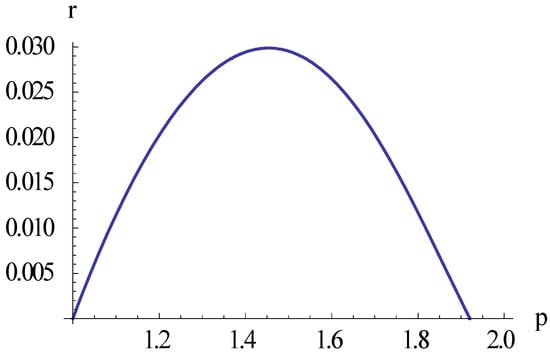
Figure 1.
The tensor-to-scalar-ratio plotted as a function of p for an inflationary model with N = 60, δns = 0.032.
We see from Figure 1 that for inflationary models with a scalar tilt given in terms of the N-fold by an equation of the form (5.24), the present ‘standard’ values of the number of N-folds and the scalar tilt, , lead to acceptable values of the tensor-to-scalar ratio, .
Equations (5.4) and (5.27) now give the potential as a function of the number of N-folds,
where .
For the special case Equation (5.27) for the tensor to scalar ratio gives
Using once more Equation (5.24) we get
which may be written
The Planck results give corresponding to . In this case Equation (5.32) reduces to
Inserting Equation (5.33) into Equation (5.7) and integrating gives
Hence
where
If the constant is chosen to be zero, the constant is represents the potential at the end of inflation as follows
With we have so this model corresponds to power law large field inflation. Lin, Gao and Gong [72] have shown that this model is only marginally compatible with the Planck results.
Koh et al. [78] have considered a class of models with
This corresponds to in Equation (5.24).
5.3. Reconstructing the Inflaton Potential from the Spectral Parameters
T. Chiba [69] has shown how one can find the inflaton potential from the spectral index. The formalism has recently been generalized to inflationary models with a Gauss-Bonnet term by Koh et al. [78].
Using Equations (3.1) and (3.51) we have
Differentiating once more we get
Hence, the slow roll parameters and are
This, together with the definitions (4.4), (4.13) and (4.29), gives
The potential as a function of N is given by the first of these equations. It can be written
Knowing V as a function of N the relationship between and N is found by integrating Equation (3.56) in the form
Chiba [69] has illustrated the method by considering a class of inflationary models where
This corresponds to the parametrization (5.24) with . With this gives in agreement with the Planck data. Inserting this into equation the first of Equation (5.46) gives
where and are constants of integration. Inserting this into the two last equations in (5.45) and introducing gives
gives which is allowed by the Planck data. For this model the -relation, and the corresponding relations involving , are
From the first of these equations we get
Inserting and gives .
Inserting (5.49) into Equation (5.42) gives
Integration with leads to
Inserting these expressions into Equation (5.46) gives
Inflationary universe models with these potentials for the inflaton field will be considered in detail later in this article and have also been studied by Kallosh and Linde [79]. The case gives inflationary models of the type motivated by supergravity, for example so-called attractor models, and will be considered in Section 6.11. The case represents the simplest chaotic inflationary models and will be presented in Section 6.1. The case will also be considered in Section 6.11.
5.4. S-Dual and Hyperbolic Inflation
Lin, Gao and Gong [72] have also considered the parametrization
where with . For this class of inflationary models
It follows from these equations that
and that
Inserting the Planck values gives . Hence requires .
Inserting the first of the expressions (5.56) into Equation (5.45) and performing the integration gives
where C is a constant. Inserting the expression (5.59) into Equation (5.46) and integrating gives
Inserting this into Equation (5.59) gives
Lin, Gao and Gong [72] have shown that these inflationary models do not satisfy the Planck/BICEP2 constraints at the 99.8% confidence level. It may be shown, for example, that with the Planck values for and N Equation (5.58) has no positive, real solution for .
The same authors have also investigated some inflationary models with the parametrization
where is a positive constant and I have replaced their by to simplify later expressions. Equation (5.46) may be written
For integration of this equation gives
Inserting Equation (5.62) gives
This leads to
where . The usual condition for a graceful exit of the slow roll era is , hence , which gives . Equation (5.66) gives the relationship
The Planck values have which requires . Assuming that and solving Equation (5.67) with these values of and r, give . In this case . A positive value of requires . For this leads to the prediction .
Lin, Gao and Gong [72] have furthermore considered the parametrization
This leads to
and
Hence,
This is similar to Equation (5.66) with . In this case the relationship takes the form
Thus, can be expressed in terms of and as
Inserting the Planck/BICEP2 data gives .
Finally Lin, Gao and Gong [72] considered the parametrization
with . Then
giving
The relationship can then be written
Here gives .
If the end of the slow roll era is defined by , i.e., we get giving
It follows from Equation (5.78) that
With this function has a minimum for giving . Hence this class of inflationary models has , which is not a realistic scenario.
5.5. The Equation of State Parameter during the Slow Roll Era
We shall now follow Mukhanov [30]. Equation (4.5) can be written
Inserting Equation (3.57) into Equation (4.13) leads to
The quantity must have a small value during the inflationary era, but not zero. A zero value means that the dominating fluid is LIVE which has constant density during the exponentially expanding era which can be represented in Einstein’s field equations by a cosmological constant. This does not provide any mechanism for a graceful exit from the inflationary era. One needs a time dependent equation of state parameter. Mukhanov [30] writes that from the very beginning of the inflationary era there should be a small deviation of the value of from zero, and the value of should be monotonously increasing during the inflation, ending with an absolute value of order 1 at the end of the era.
The usual condition for a graceful exit of the slow roll era is to require that at the end of inflation. This implies that at the end of inflation. Mukhanov has therefore proposed the ansatz
where and are positive constants of order unity. The condition at the end of inflation with gives . Gao and Gong [74] have considered inflationary models obeying the ansatz (5.82) with and replaced by .
Equations (5.80)–(5.82) give
The condition at the end of inflation requires .
We have the following cases
It follows from Equation (5.83) that
independent of the value of . A positive value of r requires . Inserting gives , while in Equation (5.85) gives , and inserting this value into the second of Equation (5.83) gives which is a little higher than required by the condition for a graceful exit of the slow roll era. Also the value of is smaller than that assumed by Gao and Gong [74].
However replacing by permits the choice of Gao and Gong. Then the modified Equation (5.85) gives
Hence implies , and gives .
As an illustration, choosing in Equation (5.83) gives
Since the first term dominates for and the second one for . Note that the value gives which is larger than allowed by the BICEP2/Planck result. Also as seen from Equation (5.84), gives too high value of r. The parameter is plotted as a function of for in Figure 2.
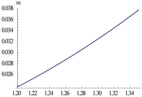
Figure 2.
The parameter δns plotted as a function of α for 1.20 < α < 1.35 with r = 0.05.
Gao and Gong [74] have applied the N-formalism and deduced the potential with the parametrization
At the end of inflation which leads to
Inserting the expression (5.86) into (5.89) gives
The value required by graceful exit of inflation, gives and
Hence with the values this class of models predicts . A positive value of requires
Thus gives .
Inserting the parametrization (5.88) into the first of Equations (5.44) and (5.47) and integrating gives
Together with Equation (5.45) this gives
and
The graceful exit value and gives and
It follows from Equations (5.93) and (5.95) that for this class of inflationary models the potential is
Myrzakulov et al. [29] have followed up the analysis of Mukhanov [30] and investigated how one can construct viable inflationary models starting from the measured values of and r and assuming the ansatz (5.82). In particular they have considered the cases and .
From the second of Equation (2.9) we have
Myrzakulov et al. [29] assume that
where is the energy density at the end of inflation. From Equations (2.1), (5.82) and (5.83) we have
With the slow roll approximation this equation reduces to
Equation (3.4) can be written
Inserting the expression (5.101) for one obtains
Integrating with leads to
The preferred value of is which gives
Following Davis et al. [80] we shall now deduce some general results for inflationary models where the inflaton field has a potential of the form
Assuming that during the slow roll era we may approximate , and by
The expressions for the standard slow roll parameters then take the form
This gives
The number of N-folds during the slow roll era is
It is usual to define the end of the slow roll era by the condition that . Hence the value of the inflaton field at the end of the slow roll era is given by
Finally we shall consider implications of a vanishing tensor-to-scalar-ratio. Biagetti et al. [81] asked “What We Can Learn from the Running of the Spectral Index if no Tensors are Detected in the Cosmic Microwave Background Anisotropy”. Here we shall consider the implications of a vanishing value of r in general for the inflationary models.
It follows immediately from Equation (4.4) that if and hence, from Equation (4.15), . From the first of the Equation (3.1) it then follows that the potential V has an extremum at the horizon crossing. It cannot be constant because that leads to a scale invariant spectrum, , which is not allowed by the Planck data.
With Equations (4.13) and (4.29) give
Since the Planck data give this equation implies that . Hence the second derivative of the potential must be negative, and the potential has a maximum at horizon crossing. Also there will be a running of the scalar spectral index only if the third derivative of the potential is non vanishing.
5.6. The β-Function Formalism
This formalism was introduced in 2015 by P. Binétruy and coworkers [82]. It was inspired by the fact that the dynamical equations of the inflationary models can be given a form similar to the renormalization group equations.
They defined a new function
Combining this with Equation (2.12) we obtain
Hence the acceleration of the scale factor is
showing that accelerated expansion requires . Combining Equations (2.20) and (5.113) we get
In the N-formalism the Hubble parameter and hence the function is given as a function of the number of e-folds, N. In this connection it is useful to note from Equations (3.7), (3.20) and (5.113) that
It follows from Equations (3.50) and (5.113) that the number of e-folds is
The inflaton field can be expressed as a function of the number of e-folds, as given in Equation (3.50), as
In this formalism the value of the inflaton field at the end of the slow roll period is determined from the condition
Let us consider an example. With Mukhanov’s choice (5.82), Equation (5.116) gives (choosing the positive square root)
where without an argument is a constant. Inserting this into Equation (5.119) and performing the integration gives
Hence
Inserting this into Equation (5.113) and integrating gives for ,
Combining Equations (2.14) and (5.113) the potential of the inflaton field is given by
Inserting the expressions (5.123) and (5.124) we get
Differentiating Equation (5.113) and using the definitions (3.7) Binétruy et al. have calculated the Hubble slow roll parameters in terms of the function and its derivatives with the result
Inserting these expressions into Equations (4.20), (4.29) and (4.44) the optical parameters may be expressed in terms of the function and its derivatives as follows
We see that is of the same order of magnitude as which is usually of the order . Assuming that the derivatives of is of the same order of magnitude as , it follows that and that we can use the approximations
With these approximations we have
According to Equations (3.50) and (5.113) the relationship between derivatives with respect to N and are
Using this the Hubble slow roll parameters can be expressed as functions of N as
To lowest order in we have
The optical parameters can be expressed as functions of N as
Using the approximations (5.130) we have
Note from Equation (5.132) that
In order to give a classification of inflationary models Binétruy et al. now assume that the potential is close to an extremal point where the field has the value , so that the -function has the following expansion,
where is a constant and . Inserting this into Equation (5.113) and integrating gives
where . Inserting these expressions for and H into Equation (5.125) gives
Sufficiently near the extremal point for . Binétruy et al. [82] have therefore used the approximation
They made a classification with seven classes of inflationary models.
- Monomial model. . Then and we can make the further simplificationCalculating the number of e-folds from Equation (5.118) then givesAccording to Equations (5.119) and (5.137) the value of the inflaton field at the end of the slow roll era isGivingInserting this into Equation (5.142) givesFrom this equation together with Equation (5.129) we obtainAssuming that this can be approximated byUsing this expression in Equation (5.134) we obtain for andHenceThe function as given in Equation (5.147) is plotted in Figure 3 for .
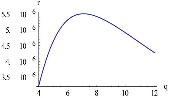 Figure 3. The tensor-to-scalar ratio plotted as function of q for β = 1 and δns = 0.032.We see that . Hence the monomial class of models predicts a practically speaking vanishing tensor-to-scalar ratio. Furthermore decreases from zero to when q increases from 1 to infinity.
 - The linear class. . From Equations (5.138) and (5.139) we then haveUsing Equation (5.118) the number of e-folds isHenceNote that with the expression (5.154) it follows that , so in this case we need the accurate expressions (5.133). This gives the optical parametersIf thenand we have the consistency relationshipsInserting gives which is much too large compared with the BPK-observations.
- Inverse field monomial class. . This is an example of large field inflation. The leading term of the function is nowIn this case the relationship takes the formwhich is plotted as a function of p in Figure 4. We see that requires .
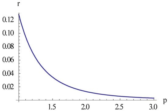 Figure 4. The tensor-to-scalar ratio plotted as function of p for β = 1 and δns = 0.032.FurthermoreHence increases from to when p increases from 1 to infinity.
 - Chaotic class, . Thenwhere . In this case integration of Equation (5.113) gives the Hubble parameterFrom Equation (5.125) we then find the potentialIn the large field case , and the potential can be approximated byUsing Equation (5.118) the number of e-folds isCombining this equation with Equation (5.161) givesThe slow roll era ends when giving . HenceWith we have , so we can approximate byUsing this in Equation (5.134) gives the optical parametersIt follows from these relationships thatandInserting gives , and . The value of the tensor-to-scalar ratio is too large to be compatible with the BPK-observations.
- Fractional class, . For this class of inflationary modelsHence gives . This prediction is in conflict with the BPK-data.
- Power law class, . In this limit the function is constant, . Integration ofEquation (5.113) then gives the Hubble parameter as a function of the inflaton fieldEquation (5.125) then gives the potentialIntegration of Equation (5.114) gives the Hubble parameter as a function of timeLetting we have a Big Bang with infinitely great Hubble parameter at the initial moment, . In this case the scale factor isHence there is power law expansion, which is the reason for the name “power law class” of this case. For this class of inflationary models the optical parameters aregivingLike the previous class of inflationary models those of this class are ruled out by the BPK-data.
- Exponential classwhere is a positive constant. This has the same form as the function of Equation (5.122) for . In this case the optical parameters areFor this class of modelsThe BPK-data, requires .
6. Predictions from Different Inflationary Models
Different inflation models have different physical motivations. However the calculations of the predictions of the models for observable quantities are usually calculated in the same way using the slow roll formalism. One often calculates numerically versus diagrams (see for example Okada et al., 2014). Then the differences between the models cook down to specifying the potential by different functions of the potential, . In this connection one often classifies the models in three classes:
Large field inflation: In these models the field strength at the end of the inflation is larger than an order of magnitude less than the Planck energy. Small field inflation: Models where the field strength at the end of the inflation is several orders of magnitude less than the Planck energy. Hybrid inflation: This is a class of models where the inflationary era ends due to an extra field different from the inflaton field that dominates during the slow roll era.
For the models that are considered in the present article we shall calculate all or some of the expressions for the spectral parameters that may be used to judge how successful the models are in relation to the Planck- and BICEP2 data and future data coming the next years. Particular focus will be put on the relationship which is well constrained by the latest observations.
There has not yet been any general agreement as to how the different inflation models should be named. I suggest that the models are given names after the mathematical form of the potential as a function of the inflaton field.
6.1. Polynomial Chaotic Inflation
The so-called chaotic inflation [83] was proposed by A. Linde [84], and is a class of polynomial inflation models. They are large field inflation models. The potential of the inflaton field in this type of inflationary models is of the large field inflation type and has a potential (Martin et al. [27] and Clesse [85],
where , and M is the energy scale of the potential when the inflaton field has Planck mass. It is assumed that p is constant and that . The class of models with and is called the inverse power-law inflation and has been investigated by J. D. Barrow and A. R. Liddle [86] and by K. Rezazadeh, K. Karami and S. Hashemi [87] in the context of tachyon inflation.
For this potential Equation (2.17) leads to
The solution of this equation with the inflaton field equal to the Planck mass at the Planck time gives the time evolution of the inflaton field during the slow roll era.
Hence, the inflaton field depends linearly upon time for . Inserting this into Equation (6.1.1) gives the time evolution of the potential,
For the time evolution of the inflaton field and the potential is
and
From Equation (2.16) it then follows that the time evolution of the Hubble parameter is
We shall now deduce expressions for the spectroscopic parameters of this model in terms of the number of e-folds. Differentiating the potential we get
The potential slow roll parameters for this model are
For this class of inflationary universe models we therefore have
Note that for . From Equation (3.22) we then get
which has been called the linear model by Kinney et al. [88]. The definition (3.7) gives in this case the equation
with the general solution
where and are constants of integration. Using Equation (2.16), we then obtain the linear relationship
Equation (3.12), on the other hand, gives in this case
with the solution
Inserting the expressions (6.1.9) into Equations (4.4), (4.13), and (4.29) we get
For this model there is also a simple expression for as given in Equation (4.32) (Amorós and Haro [56])
When comparing with the first of the expressions (6.1.17) we obtain
Equation (6.1.17) gives the and relations
With and for example we get , and . This value of r is larger than admitted by the by the BPK-data. Also these data prefer larger absolute values of and . However smaller values of may give acceptable values of . Inserting for example in the expression (6.1.20) for gives . Ballesteros and Casas [31] conclude that the single field inflationary model with a quadratic potential predicts too little running of the spectral index.
It follows from Equations (4.54) and (6.1.20) that for this class of inflationary models the running of the tensor-to-scalar ratio is
Hence
For inflationary models with the standard Bunch-Davis initial conditions for cosmic perturbations the B2014-Planck results required which gives , corresponding to inverse power law inflation.
One may also try to determine the value of p from observable data. Solving the expressions (6.1.20) with respect to p we get
Due to the large uncertainties in the measured value of and one may obtain different values of p from these expressions. With the Planck/BICEP2 2015 center values , the first expression gives .
Note for one obtains , and the slow roll condition takes the form , i.e., the inflaton field is larger than the Planck energy, making this inflationary model rather speculative as long as we lack a generally accepted quantum gravity theory.
Equation (6.1.9) gives the consistency relation (Chiba and Kohri [89])
Inserting the expressions (3.1) for the slow roll parameters one obtains the differential equation
The general solution of this equation is
where are integrations constants. Hence the consistency relation (6.1.24) is valid for all inflationary mono-field models with potential of this form.
It follows from the expressions (6.1.17) that
Hence for this class of universe models . Using Equation (4.24), Equation (6.1.27) may be written as a relation between observables
or
Together with the Planck data this formula shows that there is a problem with the polynomial inflation model. The ratio r must be positive, which requires . However the best fit Planck data are , giving , and , which is less than . Hence the Planck data and Equation (6.1.29) gives a negative value of r. As noted by Ade et al. [36] this class of inflationary models is now ruled out by the observational data.
It follows from Equations (3.43) and (6.1.28) that the ratio of the running of the spectral index of tensor and scalar fluctuations is
for the polynomial inflationary models.
It is usual to define the end of the inflationary era by . Using that , it then follows that the value of the inflaton field at the end of the slow roll era is (Remmen and Carroll, 1985)
From the first of Equation (4.1.9) we have
Hence , and during the slow roll era with the inflaton field is and .
From Equations (3.50) and (6.1.9) we have
Integrating through the slow roll inflationary era, we get
where is the value of the field strength when the slow roll era with N e-folds begins. Inserting the expression (6.1.25) for into Equation (6.1.27) it follows that the initial value of the field strength is
It then follows from Equations (6.1.9) and (6.1.34) that for an inflationary era in which the potential of the dark energy is a power of the scalar field, the slow roll parameters are
From Equations (4.13), (4.15), (4.4), (4.29) and (4.43) respectively, we then get
Hence
There is an arbitrariness in this inflationary model, because there is no mechanism determining when the inflationary era starts or ends. A start with field strength much larger than the Planck energy such as in Equation (6.1.32), does not seem very natural in the domain of a non-quantum theory. Hence, there has been proposed that the chaotic inflation period starts at the Planck time with and ends with so that can be neglected in Equation (6.1.34). Equation (6.1.35) then reduces to
Equation (6.1.1) with together with Equation (6.1.37) gives
The most simple chaotic inflationary universe model has . Typically one requires about 50-fold increase of the scale factor during the slow roll era in order to solve the monopole, horizon and flatness problems, giving .
Calculating the spectroscopic parameters, one finds that putting corresponds to neglecting p in the denominator in the expressions (6.1.36). Usual values for p and N are 2 and 50. With these values the slow roll parameters and the spectroscopic parameters will be changed only by about one per cent if p is neglected in the denominator. Therefore, the arbitrariness of the final point of time of the slow roll era in this model does not influence the predicted values of the spectroscopic parameters seriously. The expressions are then simplified to
and
The values of predicted by polynomial inflation are roughly in agreement with the value from the Planck data, but the predicted value of is more than ten times smaller than the value from the Planck data except for large values of p. Also, the quartic potential inflation model and models with higher powers of the inflaton field, are in conflict within observational data with too small predicted values of and too large values of r. The value of p can be determined by
where the first expression is calculated from Equation (6.1.37) and the second from Equation (6.1.42). For the Planck data in combination with this gives leading to a value of in conflict with the Planck data. Similarly r can be expressed in terms of N and by
giving which is larger than the value favored by the BPK-analysis (Ade et al., 2015 A).
The equations above are accurate to first order in . Creminelli et al. [12] have considered more accurate relationships valid to second order in for the case of a quadratic potential. With p = 2 the expressions (6.1.37) gives . Then Equations (4.18) and (4.19) give
From these equations we get
Hence the quantity is small to second order in . In order to obtain an -relation accurate to second order in we can therefore substitute for from the first order approximations of Equation (6.1.45) where we neglect the second order terms, i.e., and . This gives the alternative relationships
The corresponding expressions with an arbitrary value of p are
and
giving
Kobayashi and Seto [90] and Martin et al. [33] have considered inflationary models with potentials
and
They showed that with suitable values of and such models predict values of the spectroscopic parameters in accordance with observations.
Trinomial inflation with
has been thoroughly discussed by Destri et al. [91] and Martin et al. [33].
J. de Haro, J. Amorós and S. Pan [92] have studied inflationary models with the potential
where is a fixed value of the Hubble parameter at the chosen origin of time, , and we have put the cosmological constant equal to zero in their expressions. They have deduced this form of the potential from the assumption that the rate of change of the Hubble parameter with time is given by
Hence the Hubble slow roll parameters and given in Equation (3.12) are
where is the value of the Hubble parameter at the initial moment of the slow roll era. Inserting the expressions (6.1.55) and (6.1.56) into Equation (3.12) and then using Equations (4.20) and (4.29), the spectral index parameter its running and the tensor-to-scalar ratio r are
Hence, we have the relationships
For these models is given in Equation (6.1.55) as a function of H. Then it will be advantageous to write Equation (3.62) for the number of e-folds as
where is the value of H at the end of the slow roll era. Inserting the expression (6.1.55) for and performing the integration gives
with . Solving this equation with respect to gives
Inserting this into Equation (6.1.57) gives
The first of the Equations (6.1.58) and (6.1.62) may be written, respectively, as
and
Compatibility of these equations requires
or
J. de Haro, J. Amorós and S. Pan [92] required . It is usual to require that the inflationary last for between 50 and 60 e-folds in order to solve the horizon- and flatness problems adequately. In order to make some estimates we will therefore assume that . Also we will use the Planck value of the scalar optical parameter, i.e., . With these values Equation (6.1.65) gives which is allowed by the BPK-observations. Equations (5.1.63) and (5.1.64) then give respectively and . Hence positive values of α are not allowed by the observational data.
6.2. Hilltop Inflation
Think of the curve describing the potential as a function of a scalar field. The name hilltop inflation (Boubekeur and Lyth [93]) refers to the case that inflation occurs near a local maximum of this curve, i.e., near a point where . With local symmetry around this point, having , the most simple version of the potential is written (Kohri, Lin and Lyth [94])
where is a positive constant.
Inflationary models with this potential have also been called “New inflation”. Here η0 is the absolute value of the slow roll parameter at the maximum of the potential. Hill-top inflation occurs for small η0.
Hilltop inflationary models may appear as the result of considering models where the potential is a more complicated function of the inflaton field and then making a series expansion. S. Basilakos et al. [95], for example, have considered a Starobinsky-like inflationary scenario with potential
Assuming that and performing a Taylor expansion to second order in one obtains
This potential has the Hilltop form (6.2.1) with
Also it is sometimes assumed that
which may not be a good approximation in light of the Lyth relationship (4.7). With this assumption it is usual to calculate the slow roll parameters with the approximation in the numerator. This leads to
Hence, the slow roll condition requires that .
It follows from Equation (6.2.6) that in the small field case, when , then . In this case it is usual to neglect in the expressions (4.13), (4.16), (4.29) and (4.43) for and . This gives
With this approximation there is no running of the spectral index of the scalar fluctuation spectrum, . For this model the Planck result gives .
With the potential (6.2.1) the number of e-folds is approximately given by
The end of the slow roll era is given by . With Equation (6.2.6) this gives
Hence
Inserting this into Equation (6.2.6) gives
The tensor-to-scalar ratio r, the spectral index and its running for this model are
For this gives which is much larger than the value suggested by the BPK-data even when foreground dust is neglected, and .
We have seen that the small field Hilltop inflation does not give a realistic scenario. Let us therefore investigate the large field Hilltop inflation scenario in the remainder of this section. Hence, we shall now present a more accurate calculation, not making the assumption . Then it is useful to write the potential as
Here is the magnitude of the inflaton field, while is a convenient, dimensionless field variable. The slow roll parameters are
These expressions imply that
This shows that in large field Hilltop inflation, which is opposite to the small field Hilltop inflation. Combining this with the second of the Equation (6.2.14) we have
which confirms that . From the expressions (5.2.14) it also follows that
The ‘spectral index’ and the tensor-to-scalar ratio r are
Hence
This relationship is shown graphically in Figure 5.
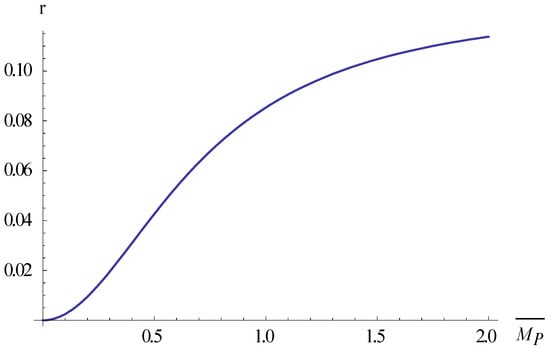
Figure 5.
The tensor-to-scalar ratio as a function of the magnitude of the inflaton field of the Hilltop inflation for ns = 0.968, η0 = 0.016 and . For larger inflaton field r approaches the value 0.128.
This equation is valid for arbitrary values of while Equation (6.2.17) is valid only for . Equation (6.2.19) may be written
which requires . The Planck and BICEP2 data, and corresponds to the largest allowed value of r in this inflationary model. The BICEP2/Planck data give .
It may be noted that this model will be ruled out if one discovers a large running of the tensor-to-scalar ration. This is seen as follows. Equations (4.50) and (6.2.19) gives
or
which requires . With the running of the tensor-to-scalar ration must obey . Hence, for example the Planck-BICEP-2014 result would rule out this class of inflationary models.
The number of e-folds is
where is the final value of the inflaton potential at the end of the slow roll era. The value of is usually determined by the condition which gives
The corresponding final value of the inflaton field is
which is much larger than the Planck energy.
We now assume that the initial value of the inflaton field is much smaller than the final value so that the first term at the right hand side of Equation (6.2.23) can be neglected. Solving the resulting equation with respect to and using Equation (6.2.24) we get
Inserting this into the expressions (6.2.18) and using the approximation , gives
which is different from the expressions in Equation (8) in Basilakos et al. [95]. It follows from the expressions in Equation (6.2.27) that
or
Hence, there is a linear relationship between r and in this inflationary model. Since , Equation (6.2.29) requires that (using )
This is the main prediction of the large field hilltop model. It is in agreement with the BICEP2/Planck data.
Inserting the expression (6.2.28) into the second of the expressions (6.2.27) gives in terms of observable quantities
Seemingly this allows a large value of since for . However, as was shown in Equation (6.2.30), this region of r is not allowed. Inserting the expression (4.2.29) for r into Equation (6.2.31) gives
This shows that . With the Planck value this gives .
Basilakos et al. [95] have considered the case , giving . However, the model in combination with the Planck results does not permit so large value of n. Inserting Equation (6.2.19) into Equation (6.2.26) and then using Equation (6.2.14) we have
showing again that in this inflationary model the inflaton field must be large, .
A more general form of the Hilltop inflaton potential has also been considered (Kinney et al. [88,96], Zarei [97] and Barenboim et al. [50]),
where is the value of the inflaton field at the extremum of the potential. It is usually assumed that . We shall first consider this case, which permits the approximation in the numerator in the expressions for the slow roll parameters. This gives
where . Hence . We shall now assume that and . Then it follows that
Inserting the expression (6.2.35) into Equations (4.13) and (4.29) we get
It follows that for this class of inflationary models the and relationships can be written
Hence that has a value close to zero in these inflation models for .
The number of e-folds is
We shall here consider a slow roll era with , so we can neglect the last term in Equation (6.2.39), which gives
Hence
From this we get [98,99]
It may be noted that for these models it is possible to obtain sufficiently small values by choosing , which are then small field models. The relation takes the form
It follows from the expressions (6.2.42) that the running of the spectral index of scalar fluctuations can be written
With and this gives which is permitted by the Planck 2015 results. Furthermore we get
giving . Inserting this, together with , into Equation (6.2.43) gives . For this gives a very small value the tensor-to-scalar ratio.
Again we shall make a more accurate calculation, this time not making the assumption . Then the slow roll parameters are
It follows from these expressions that
The corresponding differential equation is
with general solution
where A, B and C are arbitrary constants. This generalizes the potential (6.2.34).
J. Garcia-Bellido and D. Roest [70] have called the corresponding inflationary universe model with negative value of for the inverse hilltop model, while Shiu and Tye [100] and Drees et al. [101] have called it inverse power law inflation. Such a model has also been investigated by Z. Lu [102] with . Steer and Vernizzi [28] have considered an inflationary model with inverse power law potential,
With the approximation (4.2.5) their predictions are , and the -relation is .
6.3. Symmetry Breaking Inflation
There exists a so-called symmetry breaking inflation model with potential (Chiba and Khori, 2014)
This has also been called double-well inflation by Martin et al. (2013), hilltop inflation by Chiba and Khori [89], topological inflation by Chung and Lin [103], and Higgs-like by and Escudero et al. [104]. Here represents a symmetry breaking energy scale where the potential has a minimum. In the weak field case the potential (6.3.1) is often called a Higgs potential (Rehman et al. [105], but this term will here be reserved for the potential in Section 6.7.
Inserting the potential (6.3.1) into Equation (2.17) and integrating gives the time evolution of the inflaton field during the slow roll era
which is similar to that of polynomial inflation with .
For the potential (6.3.1) the slow roll parameters are
The number of e-folds for this model is (Qiu, 2014)
where the final value of the inflaton field is determined by which leads to
There is a consistency relation for this model,
Inserting the expressions (3.1) for the slow roll parameters leads to the differential equation
which may be written
Hence the general form of the potential for mono-field inflationary models fulfilling the consistency condition (6.3.6) is
where are integration constants.
Inserting the relation (6.3.6) into Equation (4.29) and using Equation (4.24) gives
With and we get which is permitted by the Planck 2015 data giving [35].
Using the expressions (6.3.3), we find that and r are
It follows that
A plot of this relationship for and is shown in Figure 6.
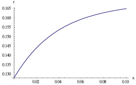
Figure 6.
Predicted values of r given in Equation (6.3.12) as a function of M for and .
Equation (6.3.10) gives . Hence this inflationary model predicts that or with the Planck data, . This is larger than the values, , favored by the BPK-data.
Solving Equation (6.3.12) with respect to M we find for the symmetry breaking inflationary models
Here gives . Hence this is an example of large field inflation.
The potential (6.3.1) can be generalized by including a non-minimal coupling to the Ricci scalar [104]. In this case the potential takes the form
where is the coupling constant. Escudero et al. [104] have shown that this model gives agreement with the Planck data if .
6.4. Exponential Potential and Power Law Inflation
In these inflationary universe models the potential is an exponential function of the scalar field [106],
Inserting this potential into Equation (2.17) and integrating with gives the time dependence of the inflaton field
With this expression in Equation (6.4.1) we get the time dependence of the potential
Differentiating Equation (6.4.2) gives
Inserting Equation (6.4.3) and the first of the expressions (6.4.4) into Equation (2.2) gives
This gives for the rate of roll,
which is constant. The class of inflationary models with a constant rate of roll has been further studied by Motohashi et al. [107].
Integrating Equation (6.4.5) with shows that the scale factor is a power function of the cosmic time,
Therefore this inflationary model has been called power law inflation [108].
Amorós and Haro [56] have noted that the potential of these inflationary models obey the condition . Inserting the definitions (3.1) for and we get the differential equation
with general solution
where A, B and C are constants of integration.
For this class of inflationary models the slow roll parameters are independent of the duration of the inflation era and have values
giving
Hence there is no running of the scalar spectral index. Equation (6.4.11) implies the relationship
In this model there is no running of the spectral indices or the tensor-to-scalar ratio. With the value from the Planck measurements we get and . Exponential inflationary models with power law expansion have mainly been considered with values of the exponent smaller than 2, which is in conflict with the Planck data. Furthermore the value of is much too high. Such exponential inflationary models are ruled out by the BPK-data, that indicate . This type of inflationary models is an example of models that fitted the preliminary BICEP2 result with a high value of r quite well [59], but that are ruled out by the recent combined BPK-results [109].
Furthermore, is should be noted that there is no natural exit of the slow roll era in the original version of the exponential inflation model.
However, in light of the Planck results S. Unnikrishnan and V. Sahni [110] have constructed a revised power law model in which inflation is driven by a scalar field with an inverse power law potential.
Geng et al. [111] have recently generalized these types of inflationary models by including an additional free parameter p so that the potential is given the form
Drees et al. [101] have considered an inflationary model with a potential having the same form, but with plus in the exponent. For the potential (6.4.13) the slow roll parameters are
Hence the scalar tilt and the scalar-to-tensor ratio r are
for . It follows that
and
Geng et al. [111] have chosen .
In the special case with we have
Hence
Inserting and gives the requirement .
Other members of the class of exponential inflationary models are the β-exponential inflationary models [112,113]. In these models the usual exponential function in the potential is replaces by the general exponential function. This introduces a new parameter which may be adjusted in order that the models shall agree with the observational data.
The hubble slow roll parameters are
The scalar spectral tilt and the tensor-to-scalar ratio are
Hence
which may be written
Inserting δns = 0.032 and r < 0.04 gives .
The value of the inflaton field, , is given by which leads to
For the number of e-folds of the inflationary era is
Inserting this into Equation (6.4.24) some nice cancellations happen, which lead to very simple, independent expressions for the spectral parameters in terms of the number of e-folds,
The last of these equations can be written
Inserting gives . It follows from Equations (6.4.26) and (6.4.30) that
With we get which is a little larger than permitted by the Planck data.
6.5. Natural Inflation
The original natural inflation potential was presented by K. Freese et al. [114] and has been further developed and compared with observational data by Freese and Kinney [115,116]. In the original model there are two variants of the potential of the scalar field generating the dark energy, given by
Here , and M is the spontaneous symmetry breaking scale. In order for inflation to occur, we must have [117]. The constant is a characteristic energy scale for the model. The potential has a minimum at and at .
Inserting the potential into Equation (2.17) and integrating we find the time evolution of the inflaton field during the slow roll era,
where K is an integration constant. We here chose . Then . This boundary condition will be chosen both for and . Then and .
Using the identity
the time evolution of the potential is found to be
Differentiating the expression (6.5.2) gives
The slow roll era starts at a flat upper part of the curve, for example at (small field inflation) or at (large field inflation). The slow roll parameters are (with the upper sign corresponding to )
where is the initial value of the field giving rise to N e-folds. The parameter represents the symmetry breaking scale and for . It follows from these relations that
The expressions (6.5.6) may be given the alternative forms
For both signs the expressions (6.5.3) give
and the consistency relations
and
From the last relation and Equation (4.29) we have
Inserting the expressions (4.24) for and gives a relation between observables for the natural inflation models
It follows from Equations (4.48), (4.50) and (6.5.10) that for this class of inflationary universe models
With and we get , .
Inserting the expressions for and in Equation (3.1) into the first of Equation (6.5.10) gives the differential equation
which may be written
The general solution is
The two potentials in Equation (6.5.1) corresponds to the special cases and , respectively.
The last of the Equation (6.5.10) on the other hand, corresponds to the differential equation
Integration gives
where A is an integration constant. The general solution is
where are integration constants.
Equation (6.5.11) leads to
which may be written
Integration gives
where K is a positive constant. Hence,
With and the plus sign this is identical to Equation (6.5.16). With the minus sign the trigonometric functions in Equation (6.5.17) are replaced by hyperbolic functions.
The spectral parameters are
It follows from these equations that
where the relationship for is the same as Equation (4.16). Since and these equations require With the value from the Planck measurements, a prediction of the natural inflation model is that . Inserting the BICEP2/Planck value gives .
The symmetry breaking parameter can be determined from observations from the first of the relationships (6.5.26),
With and we have , giving . Hence the symmetry breaking energy is much higher than the Planck energy.
Using successively Equations (4.29), (4.24), and (6.5.10) the slow roll parameter can also be determined from observations,
Hence, for this parameter is negative. For the BICEP2/Planck data we get .
The number of e-folds, with + and −, respectively, in Equation (6.5.1), are
It is usual to specify that the inflationary era ends when . Inserting in the first of the Equation (6.5.1) with we get
Inserting this into the two expressions (6.5.29) gives
or
Hence . It follows from Equations (6.5.25) and (6.5.32) that
This shows that the models with + and − in the formula (4.5.1) for the potential have the same empirical contents. These expressions are in agreement with the first of the Equation (4.5.23).
We have two limits [99],
- . Then and . This is similar to the Hilltop predictions (4.2.7) and (4.2.12). In this limit which is not favored by the Planck measurements.
- . Then and . This is similar to the predictions of chaotic inflation with . With the Planck value the prediction for the tensor-to-scalar ratio is , which is larger than favored by the Planck data.
Márián et al. [118] have recently considered Psudo periodic Higgs inflation with a potential
and shown that it corresponds well with the Planck data for a suitable value of .
6.6. Hybrid Natural Inflation
A potential problem for the original natural inflation model is that to produce sufficient inflation, the scale f of symmetry breaking must be larger than the Planck energy, and we have no accepted theory to describe such conditions where quantum gravitation effects are expected to appear.
In order to cure this potential problem, and also to provide an inflationary model with one more free parameter than the natural inflation model, thereby increasing the possibility of obtaining a model in agreement with observations, a so-called hybrid natural inflation model has been introduced. In this model the inflaton field is supplied by a second field, which is responsible for terminating inflation. This model allows for a symmetry breaking scale that is less that the Planck scale. It is also assumed that the symmetry breaking energy is not greater than the Planck energy, meaning that .
Recent investigations of hybrid natural inflation have been performed by Ross and Germán [119], Carrillo-González et al. [58], Hebecker et al. [120], Vázquez et al. [121], Ross et al. [122], and G. Germán et al. [8]. For this model the inflaton potential is written as
where is a constant with a value either or . Here represents the original natural inflation. The slow roll parameters of the hybrid natural inflation model are
where b and is defined in Equation (6.5.3). It may be noted that the relationship (6.5.6) is valid in hybrid natural inflation while (6.5.4) is not. The scalar spectral tilt and the tensor-to-scalar-ratio are
It follows from Equations (4.29), (6.6.2), and (6.6.3) that the running of the scalar spectral index is Carrillo-Gonzalez et al. [58] and Germán et al. [8],
In order to avoid quantum corrections of the potential for which we have no reliable theory, Ross and Germán [123] have considered the case that , i.e., . Then it follows from the first Equation (6.6.3) that in order to obtain a small , the parameter a must be small. Hence we can use the approximation
This shows that with (see below) we must have .
Hebecker et al. [124] have taken the initial value of the inflaton field to in order to maximize , giving and . However at this point the potential is maximally steep, so this may be said to represent “fast roll inflation” [107] rather than slow roll inflation. For slow roll inflation a more natural starting point is close to where the potential is flat. This gives and hence a value of r very close to zero (Ross et al. [119,122,123]). Let us see how close to zero. From the expressions (6.6.3) we get
With we have . From Equation (6.6.5) with we also have . Hence Equation (6.6.6) lead to the inequality
Inserting gives .
The initial value of the inflaton field can be determined in the usual way by using that the final value of the inflaton field is given by and the requirement that the slow roll era produces N e-folds. This can be calculated analytically, but the expressions are not nice. We shall therefore follow a similar procedure as that of Hebecker et al. [124], and find the initial value of the inflaton field from . This gives leading to
Hebecker et al. have used . With Equation (6.6.1) this corresponds to close to the value chosen by Hebecker et al. The slow roll parameters and the spectral parameters are evaluated with this value of the inflaton field to first order in and a (Ross et al. [122]). This gives
and
and hence,
With the values , we obtain which is a somewhat larger than the values preferred by the Planck 2015 results.
Equation (6.6.4) can be written
This expression is valid both for the original natural inflation model and the hybrid natural inflation model. But the expression (6.5.9) for leading to Equation (6.5.23) for b, is only valid for the original natural inflation model and is now replaced by the expression (6.6.12). With the BICEP2/Planck values we get a negative value for b which is not allowable. But there is a great uncertainty in the value of , namely . This encompasses , so the observational data permit a value of close to zero, giving a positive value of b. The BICEP2/Planck data then give corresponding again to a symmetry breaking energy larger than the Planck energy. Values corresponding to require approximately . Hence taking account of the the most recent observational results, also the hybrid natural inflation models seems to be in trouble unless and .
6.7. Higgs Inflation
Higgs inflation has recently been considered by Bezrukov et al. [125,126], by Gorbunov and Tokareva [127] and by Zeynizadeh and Akbarieh [128] in connection with observations of spectral properties of the cosmic microwave background radiation. Rubio [129] has given the Higgs potential as
where is a dimensionless coupling constant with value , and v is the vacuum expectation value of . The small field case has been discussed in Section 5.3.
Usually Higgs inflation is concerned with the large field potential in the second line of Equation (6.7.1). It may be noted that the potential of the Starobinsky model has the same form [97,130,131,132]. Multiplying by and neglecting the term the in the numerator, the Higgs potential is often approximated by
Differentiation of the potential (4.7.2) gives
where . In the case of Higgs inflation one usually assumes that . Hence . One therefore approximates the derivatives of the potential by
We then obtain
Hence
Using the same approximations in the calculation of the number of e-folds we have
The field strength at the end of the inflationary era is defined by , giving
Inserting this into Equation (6.7.7) gives
Equation (6.7.5) then gives
and Equations (4.13) and (4.4) then lead to
Neglecting the numbers of order unity compared to N we get
Equations (4.13), (4.15), (4.4), (4.29) and (4.43) now give
Hence, with this approximation we have the relationships
Inserting gives . These are the predictions of the Higgs inflationary models, given the Planck 2015 value of . So far these values are not in conflict with any observational results. The BICEP2/Planck results seem to favor the Higgs inflationary models.
Lyth and Riotto [22] and later Drees et al. [101] and Sebastiani et al. [130] have investigated several inflationary models with similar potentials as the one in Equation (6.7.1), for example
They assumed that the dimensionless number q is of order 1. With the same approximations as for the Higgs potential and assuming that we then find
giving
The number of e-folds is
The value of the inflaton field as given by is given by
Hence the value of the inflaton field during the slow roll era is given by
Inserting this into Equation (6.7.15) gives
This leads to the consistency conditions
For this model the Planck/BICEP2 data with give . It follows from Equation (4.54) and (6.7.22) that for this class of inflationary models the running of the tensor-to-scalar ratio is
6.8. S-Dual Inflation
This is a scenario [133] inspired by string theory. But like many other inflationary universe models it has a certain ad hoc character with some free parameters that can be adjusted so that the model cannot easily be falsified. Nevertheless the model has some nice mathematical properties. The potential is given by
where , and is a free parameter. Here the mass M characterizes the energy scale where the inflation begins. An inflationary model with this potential will be considered in Section 6.20 as an example of tachyon inflationary models. It has recently been studied by Agarwal et al. [134].
We shall here consider the more general class of potentials
where p is a real number. With we have the potential
which has been studied by Bamba et al. [65].
Calculating the slow roll parameters from the expressions (3.1) with the potential (6.8.2) gives
where b is given in Equation (6.5.3). Since we have that . Hence, it is clear that this class of inflationary universe models must be completed by adding a mechanism making it possible to have a “graceful exit” from the inflationary era.
Inserting the expressions (6.8.4) into Equations (4.13), (4.15), (4.4), (4.29) and (4.43) we find that the spectral indices of the scalar fluctuations, its running and the tensor-scalar ratio are
The expression for δns may be written
Hence δns > 0 requires either or p < 0. Note also that
Defining the end of inflation by we have
Since tanh2ϕf < 1 Equation (6.8.8) leads to the requirement b > 2/p2 or M < (|p|/)Mp. Integrating Equation (3.50) with the expression for ε in Equation (6.8.4) the number of e-folds is
in agreement with Equation (6) of Anchordoqui et al. [133]. They have argued from this equation that the requirement that there is roughly 50–60 e-folds of expansion during the inflationary era implies that , i.e., that . It follows that the standard condition for the final value of the inflaton field, and a graceful exit of the slow roll era, cannot be fulfilled in this class of inflationary models.
Note that if . The factor is the xpression for N is lacking in Equation (III.14) of Bamba et al. [65]. It follows from Equation (6.8.9) that
Inserting this equation into the first of the Equation (6.8.5) leads to
which requires . The last two equations give
Hence the inequality requires .
In their first example Bamba et al. have used the values and that represent the small field regime. This leads to and . Hence and giving and
giving
in conflict with the Planck data.
It follows from the first and third of the Equation (6.8.5) that the relationship for this class of inflationary universe models has the form,
Solving this with respect to b gives
which requires
For and this gives the condition . The value p = 1, for example, is not allowed by the PBK-data. The model with p = −1 must have b < 0.0185, i.e., M > 7.35Mp.
6.9. Hyperbolic Inflation
Basilakos and Barrow [135] have considered a class of models of inflation that is very similar to S-dual inflation. They have called it hyperbolic inflation.
We shall here consider a flat universe model in this class with radiation and inflaton energy. In this model the inflaton field has the potential
where
and w is the equation of state parameter of the inflaton energy and its mass density parameter. Furthermore , where M represents the energy scale during the slow roll era. The potential (6.9.1) leads to the following expressions for the slow roll parameters
where . Since this class of inflationary models does not have the exit problem of the S-dual models. It follows from the expression (6.9.3) that
Hence the spectral parameters of the scalar fluctuations are
The -relation is
Solving this equation with respect to we can estimate the energy scale where the inflation begins in these models from the Planck and BICEP2 data,
With for example Equation (6.9.7) gives or .
In this class of inflationary models the number of e-folds is
If the logarithmic factor is of order one, this requires that b is of the order and hence . For say this gives . Hence in order to be compatible with the Planck/BICEP2 results the energy scale of this model must be larger than the Planck energy.
The value of the inflaton field at the end of the inflationary era is defined by , giving
Hence there is a graceful exit of the inflationary era only if or which is fulfilled in the case of large field inflation. Inserting Equation (6.9.9) into Equation (6.9.8) gives
Inserting this into Equation (6.9.5) gives
6.10. M-Flation
Another string theory motivated inflation model is called M-flation [39]. In this model the potential is
where represent the energy per particle necessary to initiate inflation. The slow roll parameters are
This leads to
The slow roll period ends when . Inserting this into the first of the Equation (6.10.2) leads to a fourth degree equation for . This can be rewritten as a second degree equation by introducing a new quantity representing the inflaton field, , i.e., . Considering the region we have . Then the solution of the equation for is
Expressing the number of e-folds in terms of y we obtain
It follows from Equation (6.10.3) that
Hence, a prediction of the M-flation model is
With the Planck value this gives . In terms of the expression (6.10.3) for takes the form
Solving this equation with respect to we get
Inserting this into Equation (6.10.6) we obtain
The function (6.10.10) is plotted in Figure 7 for .
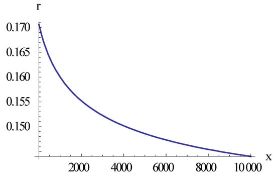
Figure 7.
The predicted values of the tensor-to-scalar ratio r by the M-flation model are here shown by plotting r as a function of for .
The expression (6.10.10) gives . Hence with the Planck value of this inflationary model predicts that which is larger than the values allowed by the BICEP2/Planck 2015 result.
6.11. Supergravity Motivated Inflation
Kallosh et al. [79,132,136] have studied a class of inflationary models motivated from supergravity, which they call attractor models. One version has potential
where , p is an arbitrary constant, and represents the characteristic energy per particle at the beginning of the inflationary era. The parameter can take any positive value. With the inflaton potential (6.11.1) the spectral index and the tensor-to-scalar ratio are given by
where , and is the inflaton field at the beginning of the slow roll era, N e-folds before it ends. Gong and Shin [137] have considered models with in this class of models and called them ‘natural cliff inflation’. In this case the expressions (6.11.2) lead to the relationship
For the Planck 2015 value this gives . Equation (6.3.11) may be written
Inserting gives b = 0.009 or .
The number of e-folds is
The end of this era is determined by . This gives
Inserting Equations (6.11.4) and (6.11.5) into the expressions (6.11.2) leads to
For and the expressions (4.11.6) reduce to
In this case the model allows small values of r in agreement with BPK-results. For and we get
These are the same predictions as those of chaotic inflation in Equation (6.1.36), and are ruled out by the BICEP2/Planck 2015 results.
The inflation models have more recently been discussed by Kallosh and Linde [138]. Among others they considered a model where the inflaton field has a potential (6.1.11) with . They also considered an attractor model with a potential similar to the one in Equation (6.7.1) for the Higgs inflation, namely
In this case and making the approximation that we can put in the numerators of the expressions for the slow roll parameters, the spectral parameters and r are
which reduces to Equation (6.7.11) for . These expressions give
Inserting gives . However, the mentioned approximation is only valid when , i.e., when . Hence the expressions (6.11.10) are not valid for large values of .
Let us calculate the corresponding expressions valid for large values of . The slow roll parameters and are
The spectral parameters and r are
These expressions lead to the following relation
This relationship is plotted as a function of in Figure 8 for with . Note that .
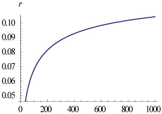
Figure 8.
The relationship (6.11.14) plotted with δns = 0.032.
The values of r shown in this figure are allowed by the Planck/BICEP2 data.
6.12. Goldstone Inflation
Lyth and Riotto [22] write that the pseudo-Goldstone boson, coming from instanton effects, is typically of the form
where and M is a mass significantly bigger than the Planck mass, . With this potential the slow roll parameters are
The final value of the inflaton field at the end of the slow roll era is given by
The number of e-folds is
where is the value of the inflaton field at a point of time with N e-folds before the end of the slow roll era. Inserting the expression (6.12.3) for into Equation (6.12.4) gives for the inflaton field at this point of time
Inserting this into the expressions (4.11.2) for and and using Equations (3.4) and (3.13) give
These expressions for and lead to
The BICEP2/Planck values and gives or , which means that this is a large field inflation model, possibly depending upon conditions outside the region of applicability of the general theory of relativity. It follows from Equations (4.29), (6.12.5) and (6.12.6) that
From Equation (3.46) we have
With the BICEP2/Planck values of r and this model gives and . Solving the last of the Equations (6.12.5) with respect to N leads to
Inserting the values of r and b gives .
It may be noted that this model is mathematically identical to one of the natural inflation models.
6.13. Coleman-Weinberg Inflation
The Coleman-Weinberg (CW) potential [139] has the form [105,140,141]
where . The shape of this potential is similar to that of the symmetry breaking potential in Figure 2, and M is the value of the field where the potential has a minimum. We shall assume that this value of the field is much less than the Planck mass, .
Two types of inflation are possible when the inflaton field has the CW potential: the large field inflation (LFI) and the small field inflation (SFI). The LFI is similar to polynomial inflation with . We shall here take a closer look at the SFI branch of the CW inflation.
We then assume that . The derivatives of the potential (6.13.1) are
Since we can approximate the second and third derivatives by
Using these expressions together with the approximation we obtain for the slow roll parameters
where . Note that since . We see that . Hence we can approximate with
The e-folding number is given by
During slow roll the quantity changes so slowly that one can approximate the integral by considering it as a constant. This gives
Using the expression for in Equation (6.13.4) we have
For this inflationary model the end of the slow roll era is given by . Since we we can neglect the last term inside the parenthesis, and obtain
Equations (6.13.5) and (6.13.9) gives
Inserting the Planck 2015 value of gives . From the expressions (6.13.4) for and , and using Equation (6.13.5) together with Equation (4.4) we obtain
Hence this inflationary model predicts that . Equations (3.21) and (6.13.11) lead to
giving .
6.14. Kähler Moduli Inflation
The Kähler moduli inflation was introduced by Conlon and Quevedo [142] and is characterized by a potential [70]
It is assumed that and hence that . We can therefore approximate the slow roll parameters and by Equation (6.2.5). This gives
The number of e-folds during the slow roll era is
Introducing a variable we find that for this gives approximately
In this model the inflaton field is assumed to be much less at the end of the inflationary era than at the beginning, . Hence
giving
Substituting from Equations (6.14.5) and (6.14.6) into Equation (6.14.2) gives
Hence , so that
With this gives . For this gives a very small value of the tensor-to-scalar ratio,
which is permitted by the BICEP2/Planck result.
With a redefinition the potential (6.14.1) takes the form
A similar model considered by Garcia-Bellido and Roest [70] has potential
with . This form of the Kähler moduli inflation was also considered by Martin et al. [33]. Then the slow roll parameters are
The number of e-folds is
where is the exponential integral, and we have neglected the lower integration limit. This function has a series expansion for large
Hence, we have approximately
Inserting this into Equation (6.14.2) leads to
giving
Again the Planck result gives . Hence and .
6.15. Hybrid Inflation
Hybrid inflation involves two fields, the so-called water fall field, , and the inflaton field, . The potential is given by [143]
where are mass parameters, and are dimensionless constants.
Rehman et al. [105] have revisited hybrid inflation in light of WMAP5 data. We shall here follow their exposition. The global minima of the potential lie at . For the only minimum of the potential lies at . In this region the potential reduces to
Note the similarity of this potential with the Hilltop potential (6.2.1). The only essential difference is the sign inside the parenthesis.
Slow roll inflation happens as the inflaton field rolls down the valley. Upon reaching the waterfall inflation ends abruptly as the inflaton field rapidly falls into one of the global minima. This scenario is termed “hybrid” because the vacuum energy density is provided by the waterfall field , while is the slowly rolling inflaton field.
With the potential (6.15.2) the slow roll parameters are
where . The spectral index and the tensor-to-scalar ratio are
It follows that
or
This requires which is just the opposite to the corresponding Hilltop requirement. Hence this model seems to be ruled out by the BICEP2/Planck result.
It follows from Equations (4.48) and (6.15.5) that the running of the tensor-to-scalar ratio is
which gives
which requires or . This, too, is opposite to the corresponding condition of the Hilltop model. Both models have difficulties in satisfying all the observational constraints simultaneously.
6.16. Brane Inflation
Several authors have considered 5-dimensional universe models where the inflationary era is due to a collision between branes [144,145,146,147,148]. This induces an effective modified gravity theory in a 4-dimensional world. We shall here follow the slow roll description as presented by Maartens and Koyoma [149].
It is usual to apply the Hubble slow roll parameters in the theory of brane inflation. However, there are some inaccuracies in the literature concerning the slow roll parameters of the brane inflation. Therefore I will here deduce the brane version of the connection between the potential slow roll parameters as defined in Equation (3.1) and the Hubble slow roll parameters as defined in Equation (3.7).
The brane version of the Friedmann Equation (2.1) takes the form
where is the tension of each brane. Differentiating this equation and using Equation (2.2) which is unchanged in brane cosmology, give the brane generalization of Equation (2.12)
Using that we obtain the brane version of Equation (2.5)
Inserting this into the previous equation gives
Inserting Equation (6.16.2) into the first Equation (3.12) we find the brane version of the first Hubble slow roll parameter
which generalizes Equation (3.7).
Using the slow roll approximation to express in terms of and we may neglect in Equation (6.16.1) which then reduces to
This gives
Inserting this into Equation (6.16.5) leads to
where ε is defined in Equation (3.1). This is in agreement with the result of Maartens and Koyoma [149].
At low energies, , the brane Hubble slow roll parameter reduce to the standard form, , but at high energies, , it takes the form
Hence in this limit .
Maartens and Koyoma have taken Equation (3.13) as the definition of . Using Equation (2.2) we then have
Inserting the brane expression (6.16.3) for we get
Note that the slow roll Equation (2.15) gives corresponding to . In order to express in terms of and we need a more accurate calculation.
Solving Equation (2.2) with respect to , differentiating with respect to time and using the expressions for and , we obtain
We now use the slow roll approximation in the following way. It is assumed that is small to the second order in the slow roll parameters and can be neglected. Also the last term is small to the second order. Furthermore assuming that is small to the first order in the slow roll parameters, we make only a second order error by neglecting in Equation (2.2) so that we can use the approximation on the left hand and in second term on the right hand side. This gives
Again we make only a second order error by using Equation (6.16.6) in this equation, giving
Using the definition (3.1) of and Equation (6.16.8) this may be written,
which is different from the corresponding Equation (6.16.8) in Maartens and Koyoma [149]. At low energies, , we have in agreement with Equation (3.22) since . At high energies, , Equation (6.16.15) gives
Hence, in this limit has much smaller values than and . With the polynomial potential above we obtain
From Equations (4.20), (6.16.9) and (6.16.16) we have
The number of e-folds during inflation is
For this reduces to
Let us consider polynomial inflation with potential given in Equation (6.1.1). The low energy regime is similar to ordinary chaotic inflation as described in Section 6.1, so we shall here consider the high energy regime with . Then Equation (6.16.20) gives
Assuming that that the inflation ends at a much lower value of the field than the initial value, we can neglect the last term, which gives
Differentiating the potential we get
Inserting this into Equation (6.16.18) gives
From Equations (6.15.19), (6.16.22) and (6.16.24) we get
in agreement with the results of Okada and Okada [148].
The Brane inflation models have a tensor-to-scalar ratio [150]
giving
rB = 24εHB,
The relationship between the tensor-to-scalar ratio and the scalar frequency index is
or
It follow from Equations (6.16.26) and (6.16.28) that
With the chaotic brane inflation model predicts . With these values of and Equation (6.16.28) gives .
It follows from Equations (4.29) and (6.15.25) that the running of the spectral indices are
For this gives .
6.17. Fast Roll Inflation
H. Motohashi, A. A. Starobinsky and J. Yokoyama [107] have investigated a class of inflationary universe models given by a potential similar to that of hybrid inflation, but with the trigonometric functions replaced by hyperbolic functions,
Essentially the same model was considered by Santos and Moraes [151]. Here is a free parameter of this class of models that interpolate between for a flat potential and for the standard slow roll approximation. Furthermore they make the ansatz,
Integration of this equation gives a relation between the scale factor and the time derivative of the inflaton field.
where is an integration constant. Comparison of Equations (2.5) and (6.17.2) gives
Substituting from Equation (2.13) for gives
Integration leads to
Determining the integration constant from gives . Then the Hubble parameter may be written as
The constant represents the energy scale at the beginning of the inflationary era when the slow roll parameters are evaluated.
Differentiating H and inserting the resulting expression for into Equation (2.13) gives
Inserting this expression into Equation (6.17.3) and choosing gives the scale factor in terms of the inflaton field
Integration of Equation (6.17.8) gives
where K is an integration constant. Hence, the inflaton field decreases with time and . With the initial condition we get . Then the inflaton field as a function of time can then be written in several useful ways,
Inserting the first of these expressions into Equation (6.17.9) gives the scale factor as a function of time,
and inserting the second of the expressions (6.17.11) into Equation (6.17.7) gives the Hubble parameter as a function of time
Note that for the scale factor of this class of inflationary models has the same time dependence,
as that of the standard universe model dominated by dust and LIVE [152].
The horizon-flow slow roll parameters can now be calculated from the definition (3.63) and the expression (6.17.13) for the Hubble parameter, giving
correcting a minor printing error in [107] in the expression for . For we get
Hence . Thus, as pointed out by Motohashi et al. [107], the even “slow roll” parameters are not small in these inflationary models.
The initial values of the slow roll parameters in the inflationary era are . Inserting this into Equation (4.57) gives
With the Planck 2015 value we get . Also we then have , and the quantity appearing in many of the expressions above, has a small value, . Then the potential (6.17.1) is close to the constant potential case represented by a cosmological constant. In this case also the even slow roll parameters are rather small, so the rolling is not so fast after all. Unfortunately this nice model is ruled out by the BKP-data due to the high value it predicts for r.
We shall now show that by taking the number of e-folds into consideration we arrive at a very similar set of predictions. Inserting the expression (16.17.13) for the Hubble parameter into Equation (3.62), performing the integration gives and utilizing Equation (16.17.11), leads to
Equation (6.17.15) shows that , so with the Planck data the final value of the inflaton field cannot be given by the usual condition . In their diagrams Motohashi et al. (2014) have considered the model during the time interval from until . Hence we determine from the first expression in Equation (6.16.11) with , giving
Inserting this into Equation (6.17.18) we get
and further inserting this into Equation (6.17.15) finally gives
For we have , and hence for we then get leading to nearly the same predictions of the spectral parameters as in Equation (6.17.17).
It seems natural now to construct a hybrid natural inflationary universe model with potential (6.5.1) instead of (6.17.1). Then the hyperbolic function in Equation (6.17.7) would be replaced by a trigonometric function. However, it may be shown that all models of this type have a negative Hubble parameter. Hence, they are contracting universe models.
6.18. Running Mass Inflation
This is a supersymmetry motivated class of inflationary models. The simplest version has the potential [153,154]
Here and are three free parameters, M represents an energy scale and is an extremum of . Defining , the slow roll parameters may be written as
Note that . The expressions (6.18.2) give
The observed values of and r can be used to restrict the parameter M and the field strenth of this class of models. Inverting the expressions for and r we get
Hence it is necessary that
Inserting the Planck/BICEP2 results gives or and .
6.19. k-Inflation
The usual models of the inflationary era describe it as a “slow roll” era where the potential energy of the inflaton field dominates over its kinetic energy and drives an accelerated and nearly exponential expansion of the universe.
In 1999 V. F. Mukhanov and coworkers [155,156] introduced a string theory inspired class of inflation models where the kinetic energy of the inflaton field, i.e., the square of the time derivative of the scalar field, drives the accelerated expansion. It was called k-inflation.
In this theory there appears a new parameter, , the velocity of the sound waves in the perturbed inflaton field. One then defines a quantity representing the ratio of the velocity of the sound waves and the ratio of the cosmic expansion,
The expression for the scalar tensor index, as given in Equation (4.56), is generalized to [157],
Lorenz et al. [158] have shown that to lowest order the tensor to scalar ratio is
From the relationship (4.15) with we then have
Tsjujikawa has discussed a model of this type with
For this model the relationship is , and the Planck 2015 value gives which is too large according to the Planck/BICEP2 data.
6.20. Dirac-Born-Infield (DBI) Inflation
This is a string theory inspired class of inflationary models. We shall here only summarize the results of Li and Liddle [157] concerning the spectral parameters of such models. They considered a class of DBI-inflationary models with polynomial potential and deduced the following expressions for the scalar spectral index and the tensor-to-scalar ratio,
Here is the sound velocity in the cosmic plasma. It follows from these expressions that
The running of the tensor-to-scalar ratio is
With we get and . These predictions are independent of the value of p. Solving the last expression in Equation (5.21.1) with respect to we get
Hence values of p between 2 and are not allowed. Further observational restrictions of the DBI-models have been discussed by Tsujikawa [159].
6.21. Fluxbrane Inflation
Taking into account radiative corrections Martin et al. [33] has argued that one can consider an inflationary model where the inflaton field has the potential
where . This has also been considered by Lyth and Riotto [22] and is called ‘spontaneously broken SUSY inflation. This model has also been considered by Guo and Zhang [160]. An inflation model with this form of the potential has also been considered by Hebecker et al. [161].
In the potential (6.21.1) is a dimensional parameter which represents the strength of the radiative effects. It is usually assumed that and . Hence we can use the approximations
for the slow roll parameters. We then get
In this case , and we can approximate by . This gives
Hence the and relations are
It follows from these expressions that
The Planck value and we get and .
With the potential (6.21.1) the number of e-folds is approximately
The value of the inflaton field at the end of the slow roll era is given by , which leads to
Hence the value of the inflaton field during the slow roll era is given by
Inserting this into Equation (6.21.4) gives
With we get which is lower than admitted in order to solve the horizon- and flatness problems.
6.22. Mutated Hilltop Inflation
B. K. Pal et al. [162,163] have introduced a new supergravity inspired model of inflation which they have called mutated hilltop inflation. In this model the inflaton field has potential
Here represents the typical energy scale for hilltop inflation, , and is a dimensionless parameter which characterizes the energy at the beginning of the slow roll era. Using the slow roll approximation in the form of Equation (2.61) the square of the Hubble parameter is
Differentiating and inserting the resulting expressions into Equation (3.7), the Hubble slow roll parameters for this model come out as
Pal et al. considered in particular the large field case with and . Then and the expressions for the slow roll parameters reduce to
Hence according to Equation (4.16), in this approximation we have
The relationship then takes the form
Hence, the running of the tensor-to-scalar ratio is
B. K. Pal et al. [162] have considered models with . With the Planck/BICEP2 value we then get a very small value for the tensor-to-scalar ratio, .
We have an approximate expression for the number of e-folds
The value of the inflaton field at the end of the slow roll era is given by , giving
Inserting this into Equation (6.22.7) gives the inflaton field during the slow roll era,
From this equation in combination with Equation (6.22.5) we get
With we get . This model is not ruled out by the Planck/BICEP2 observations.
6.23. Arctan Inflation
In a toy-model of inflation of the large field type, called arctan inflation by Drees and Erfani [101] and by Martin et al. [33], the inflaton potential is
where the mass parameter M is assumed to be much larger than the Planck mass, . It is also assumed that , so that we can let be approximated by in the in the expressions of the slow roll parameters. Defining we then get
It follows that and hence that can be neglected in the expression for . This gives
These expressions give the relationships
Hence
With the center values and of Planck 2015 and Planck/BICEP we get and . The value of is in agreement with the data so far, but Martin et al (2013) have estimated the energy scale to be which requires .
The number of e-folds is
Assuming that the value of the inflaton field during the slow roll era is given by
Inserting this into Equation (6.23.3) the spectral parameters are found to be
With the first of these relationships implies that the number of e-folds during the slow roll era is which is a little less that the optimal number for solving the horizon and flatness problems.
6.24. Inflation with Fractional Potential
Eshagli et al. [164] have investigated an inflation model in which the inflaton field has a fractional potential,
where is an arbitrary dimensionless constant. It is assumed that during the slow roll era, so that the slow roll parameters can be calculated with replaced by in the numerator in the defintions (3.1). Hence
The slow roll era ends when the inflaton field has a value . The number of e-folds during the slow roll era is
Assuming that the last term can be neglected compared to the first the value of the inflaton field during the slow roll parameter is . Inserting this into Equation (6.24.2) gives
The spectral parameters are
Neglecting the last term in the expression for this gives the consistency conditions
The running of the tensor-to-scalar ratio is
Inserting and gives and which is permitted by the BPK-data. The values of r and as functions of N are shown in Figure 9 for . Note that requires .
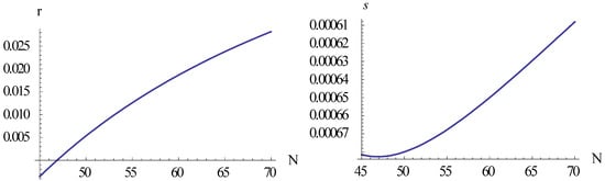
Figure 9.
The spectral parameters r and as given in Equation (6.24.6).
We see that for the tensor-to-scalar ratio is .
Two similar models called minimal Higgs inflation, have been investigated by Maity [165]. The first one has the potential
where , and is the energy scale at which the universe enters the inflationary era. Defining again the potential slow roll parameters are
Assuming that the slow roll parameters can be approximated by
It follows that . Using the approximation (6.24.10) and assuming that the number of e-folds is found to be
Inserting this into Equation (6.24.10) gives
We then obtain
For this gives a small value of , but the Planck value gives which is too small to give a realistic inflationary scenario.
The other model considered by Maity [160] has the potential
For this model the slow roll parameters are
Again we have the large field approximation
For this model the number of e-folds is
Inserting this into Equation (6.24.16) gives
Hence, we get
For this model the Planck value gives which may be acceptable. So this is a more promising model than the previous one. Also, for this model predicts a small value of r.
6.25. Twisted Inflation
J. L. Davis et al. [80] have introduced an inflationary model motivated by brane cosmology which they have called twisted inflation. The argued that the potential of the inflaton field has the form
for . Calculating the spectral parameters there will appear second order polynoms in times and times . Then it is a sufficiently good approximation to keep only the terms with . This gives
Hence
Martin et al. [33] have estimated that . This implies that the tensor-to-scalar ratio has a very small value according to the twisted inflation model. With the running of the scalar spectral index is . According to Equation (4.50) the running of the tensor-to-scalar ratio is then approximately equal to , i.e., .
6.26. Inflation with Invariant Density Spectrum
We shall here take a closer view upon the inflationary universe model with an inflaton potential of the form (6.21) giving a scale invariant density spectrum to first order in the slow roll parameters. The potential is here written as [33]
where is a free parameter. The slow roll parameters are
This shows that
Hence
This shows that the inflationary model with inflaton potential (6.26.1) has a scale invariant Harrison-Zeldovich density fluctuation spectrum.
The slow roll era ends when the inflaton field obtains a value given by , leading to
The number of e-folds during the slow roll era is
We assume that . Then, in order that , we must have either with or with . The maximal value of the function with the values (6.26.5) for is . Hence this model is ruled out as a realistic inflationary model.
6.27. Quintessential Inflation
Quintessential inflation has been considered by Md. W. Hossein et al. [166]. We shall here analyze this type of inflation by means of the N-formalism. Hossein et al. found that in the small field approximation the first potential slow roll parameter is given in terms of the number of e-folds as
where is a parameter characterizing the energy of the inflaton field during the slow roll era. In the case of small field inflation . From Equations (5.1), (5.3) and (6.27.1) we obtain
Inserting Equation (6.27.1) into Equations (5.4) and (5.7) and performing the integrations give
and
Inverting this equation gives
Inserting this into Equation (6.27.3) shows that the potential of this inflationary model is
Hence this inflationary model is mathematically similar to hyperbolic inflation with .
The expressions (6.27.2) give the consistency relation
This shows that . Hence with this model of quintessential inflation predicts which is ruled out by the BPK-data.
We shall also review three more recent versions of quintessential inflation, and consider first a model investigated by Bruck et al. [167]. The potential is
The potential slow roll parameters are
Hence the spectral parameters are,
Calculating the number of e-folds, Bruck et al. [162] have shown that
Hence,
Inserting this into Equation (6.27.10) gives
Bruck et al. (2017) have suggested that , so we can with good accuracy use the last approxomations in Equation (4.27.13). Inserting gives and .
Next we consider a quintessence inflation model investigated by Dimopoulos [34], which has a potential
where and are dimensionless, positive constants. Note that Dimopoulos et al. used a constant related to by or . Here represents the inflation energy scale, where .
The potential slow roll parameters are
The condition for the end of inflation, gives
The number of e-folds of the inflationary era is
Inserting the value (4.27.16) for gives
Hence in terms of the number of e-folds the potential slow roll parameters are
Thus the scalar spectral index and the tensor-to-scalar ratio are
Equations (6.27.20) imply that
which may be written
The last two equations gives an equation for with positive solution
which requires
Inserting gives . With we get and
Hence in this case .
Finally we consider a quintessence inflation model investigated by Agarwal et al. [134], which has a potential
For this model the potential slow roll parameters are
Hence, the spectral parameters are
The end of the inflationary era is defined by , which gives
In order to provide an analytical prediction Agarwal et al. [134] considered the case . In this case Equation (6.27.29) reduces to
Since this requires for inflation to end. In this case the spectral parameters are
This leads to
Hence which is totally unrealistic. Similar problems appear for higher values of n. Hence this class of inflationary models is ruled out by the requirement of a graceful end of the inflationary era.
6.28. Generalized Chaplygin Gas (GCG) Inflation
The GCG inflation model has recently been described by Dinda et al. [168]. We shall here give a review of their presentation.
The Generalized Chaplygin gas has a pressure which is given by the energy density as
It follows from Equations (2.1) and (2.2) that the relationship of the density, pressure and scale factor for the Friedmann universe models can be written
Inserting Equation (6.28.1) and integrating gives
For a universe dominated by Chaplygin gas behaves like a dust dominated universe model with at very early times with small values of , and as a universe dominated by LIVE with a constant density of the gas at late times with large values of . For it is opposite. Hence the case may represent the period after the inflationary era, and the case can describe the evolution during the inflationary era. Hence we assume that .
From Equations (2.1) and (6.28.1) we have
Inserting Equation (6.28.3) gives.
The first part of Equation (2.2) may be written
From Equations (6.28.5) and (6.28.6) we have
Integration gives
where is an integration constant. Equation (6.28.8) implies that . Hence may be interpreted as the initial value of the inflaton field. From Equations (6.28.6) and (6.28.3) we have
Inserting Equation (6.28.8) gives
where is the initial value of the Hubble parameter. Inserting Equation (4.28.10) into the first part of Equation (4.28.10) gives
Hence, in agreement with the equation . From Equations (2.1) and (6.29.1) we also have
Inserting Equation (6.28.11) gives the inflaton potential
where .
We now calculate the Hubble slow roll parameters. From Equations (2.28) and (6.28.10) we get
Inserting the expressions (6.28.14) into Equation (4.20) leads to
The first and last of these expressions give
which requires that 0 < m < δns. Solving Equation (6.28.16) with respect to m gives
Inserting and we get . Hence we can approximate by
The number of e-folds is
With the potential (6.28.13) we get
Since the Planck data and Equation (6.28.17) show that , the first term in the parenthesis is at least 150 times larger than the latter. Hence we can with good approximation neglect the last term during the slow roll era. This gives
or
The value of the inflaton field at the end of inflation is given by which leads to . Inserting this into Equation (6.28.22) gives
Hence the optical parameters as given in Equations (6.28.15) and (6.28.18) are
It follows that the number of e-folds is given in terms of as
Inserting the expression (6.28.17) for m we obtain
With the number of e-folds in GCG- inflation is . Since the number of e-folds is usually restricted to it is concluded that a universe dominated by generalized Chaplygin gas is not a suitable model of the inflationary era.
6.29. Axion Monodromy Inflation
We shall consider the axion monodromy inflation model with a potential [169]
A more general potential with replaced by in the first term has been considered by Minor and Kaplinghat [47]. With the potential (6.29.1) the potential slow roll parameters are
where . The BICEP2/Planck data imply that . It follows from the expressions (6.29.2) that
From the last of the Equation (6.29.2) and the first of Equation (6.29.3) we get
It follows from Equation (6.29.2) that
or
which requires . With this gives . For illustration we choose since the value chosen by Kobayashi et al. [169] is not allowed. From Equations (6.29.6) and (6.29.4) we then get . Hence and .
We shall only give a rough estimate of the upper limit of the value of N given the above values of the slow roll parameters and the constants. Since we shall neglect the term in when calculating N. This gives
Let us assume that where . Inserting this into Equation (4.29.6) we get
From this and Equation (6.29.4) we obtain
Inserting Equation (6.29.9) and into the inequality (6.29.7) gives
With we get
Inserting and gives in agreement with the observational data.
6.30. Intermediate Inflation
Intermediate inflation models were introduced by J. D. Barrow in 1990 [170,171]. I will here follow the presentations of A. Mohammadi et al. [172] and Rezazadeh et al. [173]. In both of these papers intermediate models with a no-canonical scalar field were considered. In the present review I will describe the corresponding class of models with a canonical scalar field by specializing to the case in [172] or equivalently to in [173].
The point of departure is Barrow’s assumption for the time-dependency of the scale factor,
Here A is a positive dimensionless constant, is the value of the scale factor at and where is the Planck time. It turns out that the constant A does not appear in the expressions for the optical parameters. In cold inflation its value has no consequence for the predictions of this class of models. Hence, without loss of generality we can put .
The models are called ‘intermediate’ because the expansion is faster than power law expansion and slower than the exponential expansion of the de Sitter spacetime, which has . The Hubble parameter, its rate of change and and its second derivative are
From Equations (2.1) and (2.6) together with the identity , we get
Equation (2.1) implies
Inserting (6.30.3) and integrating with the initial condition gives
Equation (2.1) also gives
Inserting (6.30.3) we get
Using Equation (6.30.5) we obtain the potential as a function of the inflaton field
For this class of models the spectral parameters are most easily calculated from the Hubble slow roll parameters (3.12) using Equation (6.30.2). This gives
Note that the slow roll parameter is a decreasing function of time for intermediate inflation. This means that there is no natural end of the inflationary era in this class of models, and one just postulates that the inflationary era lasts for a suitable number of e-folds, say . In this class of models one defines instead the beginning of the inflationary era by the condition , and evaluates the spectral parameters at the end of the inflationary era. However, Rezazadeh et al. [173] have invoked a non-canonical scalar field in order to solve the exit problem for intermediate inflation.
Using Equation (6.30.5) the slow roll parameter is expressed in terms of the inflaton field as
It follows from Equations (3.46) and (6.30.1) that the number of e-folds is
where is the initial point of time of the inflationary era, defined by giving
Inserting this into Equation (6.30.11) gives for the point of time when the slow roll parameters are evaluated
Giving
The spectral parameters , and are expressed in terms of the Hubble slow roll parameters in Equation (4.20). Inserting the expressions (6.30.14) we obtain
Note that the curvature spectrum is scale independent, corresponding to , for . The expression for corrects an error in Mohammadi et al. [172]. For these model the relationship is
The constant can be expressed in terms of and as
Inserting the last expression into Equation (6.30.16) gives
With the Planck values and we get . This value of r is larger than permitted by the Planck observations. However the more general models with non-canonical inflaton fields studied by Mohammadi et al. [172] and Rezazadeh et al. [173] contain an additional adjustable parameter in the expressions for the observable parameters, making agreement with observational data possible. A class of intermediate inflationary models with a variable sound velocity have recently been investigated by N. Nazavari et al. [174]. In these models one may obtain agreement with the Planck data. Below we shall consider warm intermediate inflation models, and they lead naturally to a suppression of the curvature perturbation, giving a small value of r.
Brane-Intermediate Inflation
S. del Campo and R. Herrera [175] have investigated observable consequences of intermediate inflation on the brane. The scale factor is given in Equation (6.30.1), and the Hubble parameter and its derivatives in Equation (6.30.2). Inserting these expressions into Equation (6.16.16) gives
Integrating with leads to
From the expressions (6.30.2) and Equation (6.16.19) we get
From Equations (6.30.19) and (6.30.20) the potential is
The brane tension is usually assumed to be very small in Planck units, so in the strong field case the first term inside the brackets dominates. Hence we can approximate the potential with
which has the same form as in polynomial inflation with . However the predicted values of the spectral parameters are different from those of polynomial standard inflation since the dynamical equations are different in brane-inflation.
The Hubble slow roll parameters as functions of time are the same as in standard inflation, and are given in Equation (6.30.9). Combining these expressions with Equation (6.30.20) gives
The inflaton field at the end of the inflationary era is given by , giving
The number of e-folds during the slow roll era is found by combining Equations (6.30.11), (6.30.19), (6.30.23) and (6.30.24), giving
In spite of the different time dependence of the inflaton field for the standard intermediate inflation and the brane-intermediate inflation the expressions for the slow roll parameters are identical. The reason is that they depend only upon the time dependence of the scale factor.
However the expressions (4.20) are modified, so Equations (6.30.15)–(6.30.17) are not valid for brane-intermediate inflation. Del Campo and Herrera [175] have shown that
Inserting the expressions (6.30.25) gives
or
Inserting and gives . This is a little smaller that the values del Campo and Herrera arrived at with the observational data up to 2009.
Del Campo and Herrera found that the running of the scalar index is
giving in agreement with observational data. They found that the tensor-scalar ratio is given by
Inserting the expressions (6.30.9) into Equation (6.30.26) leads to
It follows from the last two equations that the relation is
With we get . From the above result a proper choice of is . Furthermore we insert the favored Planck value . Recently J. R. Gott III and W. N. Colley [46] have shown that from the best available data it follow that . Inserting these values into Equation (6.30.32) gives .
6.31. Constant- Roll Inflation
H. Motohashy, A. A. Starobinsky and J. Yokoyama [107,176], F. Cicciarella, J. Mabillard, J and M. Pieroni [177] and A. Karam et al. [178] have recently considered a class of inflationary models with constant rate of roll. They defined the ‘rate of roll’ as . According to Equation (3.16) this is the same as minus the Hubble parameter . Hence the general condition for constant rate of slow roll inflation may be written
where , and are constants, is used in [107], in [171] and in [172]. It follows from Equations (2.5) and (3.16) that
Hence, the case or , and implies that constant, i.e., it represents a flat potential. We shall first consider this case.
With Equation (3.7) takes the form
The general solution of this equation is
Differentiating Equation (6.31.4) and using Equation (2.14) we have
showing that V is indeed constant. In this case Equation (3.12) takes the form
Integration gives
where is an integration constant. It follows from Equation (2.12) that . Integration of Equation (6.31.7) then gives
where K is a new integration constant. Equation (3.16) now reduces to
Using that and integrating gives
where is an integration constant.
Integration of Equation (6.31.8) with and leads to
where is an integration constant. Inserting this into Equation (4.31.10), determining the integration constants from Equation (2.12), and assuming that the inflaton field decreases with time gives
a(t) = a1sinh1/3(3H1t).
New integration with gives
Differentiating Equation (6.31.8) gives
Inserting Equations (6.31.12) and (6.31.14) into Equation (2.12) gives . Equation (2.2) then gives
which is constant. Comparing with Equation (6.31.5) we get . The Hubble slow roll parameters,
The scalar spectral index is small only at a certain point of time, t1, when , so this is not a realistic inflationary model.
We shall now consider the corresponding models with , i.e., . The case i.e., corresponds corresponds to the scale invariant case which is in conflict with observation, so this case will not be considered here. Equation (3.7) now takes the form
The general solution is
Equation (6.31.5) is now generalized to
Motohashy, Starobinsky and Yokoyama [107] have considered 3 special cases.
- (1)
- givingIn the case a positive potential requires .For the potential is recognized as that of power law inflation. Comparing with Equation (6.4.1) we have . From Equations (6.4.7) and (6.4.8) we then get and hence . This value of is higher than allowed by the Planck observations.
- (2)
- giving
- (3)
- giving
It may be noted that the expressions (6.31.23) and (6.31.25) for are similar to those for natural inflation as given in Equation (6.5.1). The predictions of the model with has been compared with the Planck data by Motohashi and Starobinsky [176].
In this case Equation (3.12) takes the form
Hence, the generalization of Equation (4.31.7) is
Integrating this equation we have to consider some cases.
1. Let us first consider the case . Integration of Equation (6.31.27) then gives
Then the special case gives the constant Hubble parameter of a universe with exponential expansion such as the De Sitter spacetime dominated by a Lorentz Invariant Vacuum Energy (LIVE) with a constant density that may be represented by a cosmological constant.
A flat universe FLRW-universe dominated by a perfect fluid with equation of state has a Hubble parameter
Hence, putting in Equation (6.33.28) gives the Hubble parameter of a flat FLRW-universe dominated by a perfect fluid with equation of state parameter
The condition interpolating between LIVE and a Zel’dovich fluid restricts to the interval .
2. Next we consider the case . Then Equation (6.31.27) takes the form
Since is negative requires , and requires . Solving Equation (6.31.31) with these requirements in mind leads to
3. Finally we have the case . Then
which requires . The solution of Equation (6.31.33) is
Integrating the expressions for the Hubble parameter we get the time evolution of the scale factor. We shall only consider the cases 2 and 3. From Equation (6.31.32) with we obtain
It was noted by Motohashi et al. [176] that also in this case the expression for the scale factor in the case corresponds to that for a flat FLRW model with a cosmological constant filled with a perfect fluid with equation of state , where . Hence the case corresponds to the standard ΛCDM universe model.
From Equation (6.31.34) with we get
The cases 2 and 3 behave in a similar manner for small values of . Hence from now on we shall only consider the case 2.
Equation (3.13) then takes the form
giving
For the case 2 we now get
while the case 3 leads to
Integration of Equation (6.31.39) gives
and of Equation (6.31.40),
Differentiating Equation (6.31.32) gives
The time dependency of the inflaton field in the case 2 is
Inserting the expressions (6.32.41) into (6.31.44) gives the inflaton potential for the case 2
The Hubble slow roll parameters for this case are
The tilt of the scalar spectral index and the tensor-to-scalar-ratio are
In all cases the relationship is
The preferred values from the Planck observations, give . Hence the case is favored with . The values and are not permitted. The observational constraint , gives the restriction .
A related class of inflationary models, called ‘constant slow-roll inflation’, has been considered by Gao and Gong [74]. They are defined by the condition that the slow roll parameter η defined in Equation (3.1) is constant, hence
Integration gives
These are power law inflation with exponential potential, linear polynomial inflation and natural inflation.
One may use the N-fold formalism to investigate this class of inflationary models. Integrating Equation (5.44), i.e.,
gives
where A and B are constants of integration. Integrating Equation (3.58), i.e.,
with the boundary condition gives
Hence the tensor-to-scalar ratio is
The scalar spectral tilt is
The two last equations give
From Equations (6.31.54) and (6.31.56) we get
Inserting gives and . Hence, among the 3 classes of models in Equation (6.31.49) the one with is favored by the observational data. We shall therefore consider this class of models.
It follows from Equation (3.50) that the inflaton field is given in terms of the number of e-folds by
Inserting the expression (6.31.54) we find
which is different from Equation (12) of Gao [74]. Inserting the expression (6.31.60) into Equation (6.31.50) and choosing gives
This is the form of the potential of the natural inflationary models.
Cicciarella, Mabillard and Pieroni (CMP) [177] have recently applied the function formalism to the constant rate of roll inflationary models. It follows from Equations (5.127) and (6.31.1) that the condition for constant rate of roll inflation can be written in terms of the function as
It follows from Equations (5.128) and (6.31.62) that for these models the scalar spectral index and the tensor-to-scalar ratio are related by
CMP [177] have integrated Equation (6.31.62) for different cases.
1. De Sitter and chaotic models, . In this case there are two solutions.
1A. . Equation (5.112) then gives a constant Hubble parameter, with exponential expansion, . This represents the De Sitter spacetime. In this case the condition is never obtained, and therefore there is no end to the slow roll era.
1B. . This is a member of the chaotic class of Binétruy et al. [82] with properties described in the Equations (5.159)–(5.169).
It follows from Equation (6.31.33) that the models 1A and 1B have and are ruled out by the BPK-data.
2. Constant function, . It follows from Equation (6.31.61) that in this case with . This is a member of the power law class of Binétruy et al. [82]. In this case , so this model is ruled out by the BPK-data.
3. Fast roll inflation. General case with . This class of models will be discussed in Section 6.17. For these models Equation (6.31.63) gives , so they are ruled out by the BPK-data.
4. Interpolating model with . In order to simplify the expression we introduce in this case a constant by . It follows from Equation (6.31.63) that the BPK-data, require or . In this case the solution of Equation (6.31.62) may be written
Hence this model Interpolates between the linear class of models described in Equations (5.150) to (5.157) and the class of chaotic models, respectively in the limits and . Inserting the expression (6.31.64 ) into Equation (5.113) and integrating gives the Hubble parameter
and inserting the expressions (6.31.64) and (6.31.65) into Equation (5.125) gives the potential
where . Inserting the function (6.31.64) into Equation (5.118) gives the number of e-folds
It follows from the condition for the end of the slow roll era that
Inserting Equations (6.31.67) and (6.31.68) into Equation (6.31.64) gives
Inserting this into Equation (5.134) we get for and r
It follows from these expressions that
The BPK-data, require .
6.32. Warm Inflation
In the usual (cold) inflationary models dissipative effects with decay of inflaton energy into radiation energy are neglected. However, during the evolution of warm inflation dissipative effects are important, and inflaton field energy is transformed to radiation energy. This was first taken into account in the construction of inflationary universe models by A. Berera [179] who introduced a new class of inflationary universe models called Warm Inflation. Further references to works prior to 2009 on warm inflation are found in [180,181]. For later works see [182,183,184] and references in these articles. The most recent articles are [185,186]. In this scenario there is no need for a reheating at the end of the inflationary era. The universe heats up and becomes radiation dominated during the inflationary era, so there is a smooth transition to a radiation dominated phase.
6.32.1. General Warm Inflation Equations
During the warm inflation era both the inflaton field energy with density and the electromagnetic radiation with energy density are important for the evolution of the universe. The Friedmann Equation (2.2) is generalized to
In these models the continuity Equation (2.3) for the inflaton field and the radiation take the form
respectively, where is a dissipation coefficient of a dissipative process which causes decay of dark energy into radiation. In general is temperature dependent. It follows from these equations that the evolution equation for the inflaton takes the form
in the case of warm inflation.
During warm inflation the dark energy predominates over radiation, i.e., . During inflation and are slowly varying and the production of radiation is quasi-static, . Then Equations (2.2), (6.32.2) and (6.32.3) take the form
Hence in these models all of the radiation energy during the inflationary era comes from dissipation of the inflaton energy. In orther words, without dissiopation there is no radiation energy in the slow roll approximation. The last equation may be written as
Here Q is called the dissipative ratio. Using Equation (6.32.2) the energy density of the radiation during warm inflation is given by
where Cγ is a constant and T is the temperature of the radiation. The last two equations together with the slow roll approximation 3H2 = κV lead to the following expression for the temperature of the radiation
It follows from this equation and the first of the equations in (6.32.4) that the ratio of the energy densities of the radiation and the inflaton field are
Differentiating the first of Equation (6.32.4) and using that we get . Inserting the expression for from Equation (6.32.6) leads to
Hence we get
The Hubble slow roll parameters are
giving
This shows that during the slow roll era the energy density of radiation energy is much less than the the energy density of the inflaton field.
In the warm inflation scenario a thermalized radiation component is present with temperature , where both T and H are expressed in units of energy. Then the tensor-to-scalar ratio is modified with respect to standard cold inflation, so that [187]
Hence, the tensor-to-scalar ratio is suppressed by the factor compared with the standard cold inflation.
Hall, Moss and Berera [188] have calculated the spectral index in warm inflation for the strong dissipative regime with or . We shall here follow Visinelli [189] and permit arbitrary values of . Equation (6.32.9) can be written
which replaces the corresponding cold inflation Equation (2.12). Using Equations (3.1), (6.32.4), (6.32.6), (6.32.14) and finally (6.32.9) we get
The Hubble slow roll parameters can be written
Hence
During the inflationary era the energy density of the radiation is much less than the energy density of the inflaton field, . Using Equation (6.32.12) this condition takes the form
In the strong dissipation regime this reduces to .
Hall, Moss and Berera [190] have defined the end of the slow roll era for warm inflation by the condition which in the strong dissipation regime corresponds to . Note that means and therefore . Hence for these models inflation ends with a transition from accelerated expansion to linear expansion, like that of the empty Milne universe.
Differentiation of Equation (6.32.6) and using that gives
Dividing by and using the first of Equation (6.32.4) in the two last terms lead to
Using Equation (6.32.19) we get
in agreement with Equation (2.14) of Visinelli [189]. Hall, Moss and Berera [190] and Rezazadeh et al. [173] have calculated that in the strong dissipative regime the scalar spectral index parameter, the tensor spectral index and the tensor-to-scalar ratio are
where is the Stefan-Boltzmann constant.
It may be noted that in warm inflation the condition for slow roll is that the absolute values of and are much smaller than .
Moss and Xiong [191] have deduced a general expression for the scalar spectral tilt in warm inflation, and Herrera [192] has shown that when the dissipation coefficient is independent of the temperature, their expression takes the form
In the weak dissipative regime this expression reduces to
6.32.2. Warm Polynomial Inflation
Visinelli [193] has investigated warm inflation with a polynomial potential which we write in the form
where since the potential and the inflaton field have dimension equal to the fourth and first power of energy, respectively. Here M represents the energy scale of the potential when the inflaton field has Planck mass. Furthermore he assumes that the dissipative term is also monomial
He considered models with and . However in the present article we shall also consider polynomial models with . Note that corresponds to a constant dissipation coefficient.
From Equations (6.32.25) and (6.32.26) we have
The constant represents the strength of the dissipation. For the dissipative ratio is constant, . We shall here consider the strong dissipative regime where . Then the third of Equations (6.32.4) reduces to
Inserting Equations (6.32.25) and (6.32.26) gives
Integration leads to
where K is a constant of integration. The initial condition gives .
The special cases (i) , i.e., and (ii) , i.e., , both with the initial condition , i.e, , have been considered by Sharif and Saleem [194]. The latter case was originally considered by Taylor and Berera [195]. For these cases the condition requires . In the first case Equation (6.32.32) reduces to
Note that the time has dimension inverse mass with the present units, so that is dimensionless.
Visinelli, however, has considered polynomial models with . Then we have to change the initial condition. The corresponding solution of Equation (6.32.31) with and the inflaton field equal to the Planck mass at the Planck time gives
It may be noted that gives a different time evolution of the inflaton field. Then Equation (6.32.29) with the boundary condition has the solution
In this case the inflaton field decreases or increases exponentially, depending upon the sign of .
Inserting Equations (6.32.25) and (6.32.27) into Equations (6.32.15), (6.32.20) and (6.32.21), the slow-roll parameters are
With these expressions Equation (6.32.23) valid in the regime of strong dissipation, , gives
The slow-roll regime ends when at least one of the parameters (6.32.34) is not much smaller than . In the strong dissipative regime and . Using Equations (6.32.27) and (6.32.34) we then get
The number of e-folds, N, in the slow roll era for this model has been calculated by Visinelli [193]. It is defined by
Using Equations (6.32.4) and (6.32.6) we get
Inserting the potential (6.32.25), performing the integration and considering the strong dissipative regime, gives
The time dependence of the inflaton field is given by Equation (6.32.32) when showing that in this case, and by Equation (6.32.32) when implying in that case, showing that in both cases.
Inserting this into the first of Equation (6.32.34) and Equation (6.32.27) gives
Inserting these expressions into Equation (6.32.35) gives
Note that with , i.e., a constant value of the dissipation parameter , this equation reduces to
for all values of p. Then gives which is smaller than the preferred value from the Planck data, . Inserting in Equation (6.32.44) and solving the equation with respect to p gives,
The Planck values give and , and hence is negative in conflict with the Planck observations.
Panotopoulos and Videla [183] have investigated the tensor-to-scalar ratio in this model with . According to Equation (6.1.36) in this case for cold inflation. For this corresponds to which is an acceptable number of e-folds. Then Table 1 shows that the tensor-to-scalar ratio is , which is much larger than allowed by the Planck observations. Furthermore, in this case case . Panotopoulos and Videla found the corresponding relation in warm inflation with , where a is a dimensionless parameter. They considered two cases.
A. The weak dissipative regime. In this case and Equation (6.32.13) reduces to . They then found
With and this requires . However, they also found that in this case giving which is too small to be compatible with the standard inflationary scenario.
B. The strong dissipative regime. Then and . They then found
Then and , so this is a promising model.
Taylor and Berera [195] have briefly considered warm inflation models with an exponential potential, , and found that in the strong dissipation regime the scalar spectral index parameter for models of this type is
and hence is negative in conflict with the Planck observations.
6.32.3. Warm Natural Inflation
Visinelli [188] has investigated warm natural inflation with potential
Here , and M is the spontaneous symmetry breaking scale. He assumed that the dissipation coefficient is independent of the inflaton field, so that . Inserting the definitions of and into Equation (6.32.23) then gives
Inserting the potential gives
where is given in Equation (6.5.3). From the first of the Equation (6.32.4) with the potential (6.32.48) we have
Equations (6.32.5) and (6.32.51) then give
Hence
We shall now express the in terms of the number of e-folds of expansion during the slow roll era for this inflationary universe model, again following Visinelli. Assuming that the dissipation parameter is independent of , i.e., that , the number of e-folds is given by
Differentiating the potential (6.32.48) and inserting Equation (6.32.51) we get
Hence,
Visinelli has argued that
giving
Inserting this into Equation (6.32.56) gives
Applying the trigonometric identity
in the expression (6.32.59) and inserting the result into Equation (6.32.53) we finally arrive at
Here we must have in order to give the Planck value for . Hence, Equation (6.32.59) gives . A good approximation for is therefore
Inserting and gives .
Visinelli [188] found that the tensor-to-scalar ratio for this inflationary model is
Differentiating the expression (6.32.51) gives
Combining this with Equation (6.32.14) in the strong dissipative regime and using Equation (6.32.5) gives
The energy density of the radiation is
where a = 7 × 5657 × 10−16 J·m−3·K−4 = 4.69 × 10⁻⁶ GeV·m−3·K−4 is the radiation constant. Combining with Equation (6.32.7) we get
Equations (6.32.63), (6.32.65) and (6.32.66) give
Visinelli [188] has evaluated the constant B and concluded that for this type of inflationary universe model the expected value of r is extremely small. If observations give a value this model has to be abandoned.
6.32.4. Warm Viscous Inflation
As noted by del Campo, Herrera and Pavón [196], it has been usual, for the sake of simplicity, to study warm inflation models containing an inflaton field and radiation, only, ignoring the existence of particles with mass that will appear due to the decay of the inflaton field. However, these particles modify the fluid pressure in two ways: (i) The relation between pressure and energy density is no longer as it is for radiation. A simple generalization is to describe the mixture of matter and radiation as a fluid with equation of state , where is the adiabatic constant with value . (ii) Due to interactions between the particles and the radiation there will appear a bulk viscosity so that the effective pressure takes the form , where
is a “viscous pressure” and a coefficient of bulk viscosity.
Following Setare and Kamali [197] the second of the Equation (6.32.2) is now generalized to
With quasi static production of radiation we have and . The Equation (6.32.70) reduces to
Equations (3.7) and (6.32.9) give
Using Equation (6.32.1) with we get
Let us for a moment consider the strong dissipative regime with . Then Equation (6.32.73) reduces to
In this case we get
Hence the slow roll condition requires that
6.32.5. Warm Viscous Intermediate Inflation
We shall now consider the warm, viscous, intermediate inflation models studied by Setare and Kamali [197] in the strong dissipation regime. This is also similar to the isotropic universe models corresponding to the anisotropic models considered by Sharif and Saleem [194]. The scale factor is given in Equation (6.30.1) and the Hubble parameters and its derivatives are given in Equation (6.30.2), where the expressions must be multiplied by A in the present case. In order to find the time evolution of the inflaton field we now write Equation (6.32.9) as
Inserting the expression (6.30.2) for into Equation (6.32.77) gives
where is the Planck time. Note that this requires .
Both Setare and Kamali [197] and Sharif and Saleem [194] have considered two cases. In the first one assumes
Equations (6.32.4) and (6.32.5) then give
Furthermore, for several reasons, the authors restricted their analysis to the strong dissipative regime where . Equations (6.32.77) and (6.32.78) then reduce to
where we have used Equation (6.30.2). Integrating with the initial condition and assuming that we get
which is different from the corresponding Equation (6.31.5) for cold intermediate inflation. We see that is an increasing function of time. Inserting the expression (6.30.2) for H into the first of the Equation (6.32.4) gives
Hence the potential decreases with time. Combining this with Equation (6.32.82) leads to
Inserting the expressions (6.32.79) into Equation (6.32.71) we obtain
Hence in order that the density of the mixture of matter and radiation shall be positive, we must have . Inserting the expressions (6.30.2), (6.32.81) and (6.32.83) we find the evolution of the density with time,
Solving Equation (6.32.81) with respect to time gives
Inserting this into Equation (6.32.86) gives the density as a function of the inflaton field,
Setare and Kamali [197] and Sharif and Saleem [194] used the Hubble slow roll parameters (3.7). In the strong dissipative regime with they take the form
Furthermore Setare and Kamali have shown that for this type of inflationary models the scalar spectral index parameter is given as
Differentiating the expression (6.32.83) gives
Inserting the last expression for into Equation (6.32.91) gives
Together with the expression (6.32.91) for this leads to
Note that the scale independent Harrison-Zeldovich spectrum occurs for .
The slow roll era ends when the inflaton field has a value so that , corresponding to , which gives
The number of e-folds is given by Equation (6.32.40), which in the present case takes the form
Inserting the potential (6.32.84) and integrating gives
Hence
Inserting Equation (6.32.97) into Equation (6.32.93) leads to
A positive value of requires . Equation (6.32.98) can be written
Inserting the Planck value and gives . This is in conflict with the requirement . The values give which is smaller than allowed by the BPK-data.
In the second case Setare and Kamali and Sharif and Saleem assumed that . Equation (6.4) then takes the form. Using Equations (6.32.79) and (6.30.2) and integrating with the initial condition , leads to
where . Hence from the first of the equations Equation (4.32.4) we have
From Equations (6.32.1) and (6.32.100) the viscous pressure is
In the present case Equation (6.32.84) is replaced by
Differentiation the first of Equation (4.32.100) we have
Inserting this, together with the expression (6.31.2) for H into Equation (6.32.103) gives the time evolution of the density of the matter-radiation fluid,
Substituting for t from Equation (6.32.99) we obtain the density as a function of the inflaton field
In this case and becomes
The expression for is different for that of Setare and Kamali and will lead to a different conclusion than their concerning the acceptability of this class of inflation models. Inserting the expressions (6.32.107) into Equation (6.32.89), the scalar spectral index is
Hence,
The final value of is given by
The number of e-folds is
Hence
The scalar spectral index is
which can be written
Inserting the Planck value and gives . This is outside the range allowed by Equation (4.32.78), , which requires . Hence these models are not acceptable for realistic inflation. However in the anisotropic case considered by Sharif and Saleem, one may obtain agreement with the Planck data for . The tensor to scalar ratio has a very small value in these models.
In the case (i) considered above the dissipation coefficient is assumed to be proportional to the potential of the inflaton field, . Combining this with the first of Equations (6.32.4) we get . Furthermore in the strong dissipative regime with this leads to . With these models have .
The slow roll era begins at a point of time when the inflaton field is given by Equation (6.32.81). Combining this with Equation (6.32.73) leads to
With we get . A smaller value of corresponds to a later beginning of the inflationary era.
V. Karmali and Setare have considered warm viscous inflation models in the context of brane cosmology using the so-called chaotic potential (4.1.1) with . The corresponding models in ordinary (not brane) spacetime correspond to taking the limit that the brane tension in their equations. They first considered the case . Then the time evolution of the inflaton field is given by Equation (6.31.5) with . In this case which is smaller than the preferred value from the Planck data. Karmali and Setare got a different result. Letting in their Equation (68) gives , i.e., a scale invariant spectrum.
Next they considered the case where is a dimensionless constant. With this corresponds to the first case considered by Sharif and Saleem. It will now be shown that this model is in conflict with observations. With we then have . In the strong dissipation regime: . Hence , giving .
We now use the constraints from the Planck satellite data, . This gives a lower bound on as Hence the model with is in conflict with the Planck data.
6.32.6. The N-Formalism Applied to Warm Inflation
We shall here follow the paper of R. Herrera [192] and use units so that . In warm inflation the relationships of the derivatives of V with respect to and N, the first one corresponding to Equation (5.42) in cold inflation, are
Furthermore for the derivatives of the dissipation coefficient with respect to and N we have
Hence the potential slow roll parameters of warm inflation as given in Equations (6.32.15), (6.32.20) and (6.32.21) take the forms
The Equation (6.32.23) for the scalar spectral tilt can then be written
or using that ,
Since in the slow roll approximation we obtain
Using Equations (6.32.4) and (6.32.118) it follows that Equation (6.32.13) for the tensor-to-scalar ratio for warm inflation takes the form
I follows from Equations (3.62), (6.32.4), (6.32.5) and (6.32.116) that
From Equations (6.32.7) and (6.32.116) we have
Hence the tensor-to-scalar ratio is
In the weak dissipative regime where , the relation can be written
Using Equations (5.32.124), (6.32.121) and (6.32.122) then reduce to
In the strong dissipative regime where , the relation can be written
Then
Note that the only difference between the expressions for and in terms of in the weak and strong regime is that . It follows from Equations (6.32.127) and (6.32.129) that the potential is in both cases given by
Herrara [192] has considered a few examples. In the first one
In this case the relation is
The observational result that then leads to the requirement
Insering gives .
Equations (6.32.130) and (6.32.131) give the potential as a function of N
where A is a constant. Inserting this into Equation (6.32.126) gives in the weak regime
From the last two equations we have the potential
In the strong regime Equations (6.32.128) and (6.32.129) lead to an integral that cannot be solved in terms of elementary functions.
In the special case that we have the prediction and , i.e., Equation (6.32.130) then gives . Then we get from Equation (6.32.126) . Hence in this case the potential is
The expressions for cold inflation corresponding to those in Equation (6.32.131) are found in Equation (6.1.42). For these models require a value of the exponent less than 0.3, but warm inflation gives generally a smaller value of r than the corresponding cold inflation models.
6.33. Tachyon Inflation
So called tachyon inflation is a string theory inspired model of inflation where the action has a certain form [28,61,198,199]. Although it has been shown by Kofman and Linde [200] that there are certain problems with tachyon inflation, it is considered here because it also has some nice properties. A recent analysis leading to observational constraints on tachyon inflation has been presented in [201].
6.33.1. General Tachyon Inflation Equations
In these models it has become usual to introduce a so-called tachyon field and denote it by . A rolling tachyon field [202] can be described as a fluid which in the homogeneous limit has energy density and pressure
where is the tachyon potential. Hence [194],
showing that the tachyon matter interpolates smoothly between LIVE for and dust for .
The equation of motion of the tachyon field is
where we use the notation .
For this class of models Friedmann’s first and second equations take the form
There will be accelerated expansion when . Inserting Friedmann’s first equation gives
Since Equation (6.33.5) may also be written as
It follows that [199]
Inserting (6.33.7) into (6.33.6) gives
Using Equation (6.33.7) this equation takes the form
It follows from Equations (6.33.4) and (6.33.5) that Hubble slow roll parameters are
Hence a time independent tachyon field behaves as LIVE and gives exponential expansion, while integration of Equation (6.33.8) with a tachyon field having gives which is the behavior of a dust dominated universe. As emphasi zed by Gibbons [194], if the tachyon condensate starts to roll down the potential with small initial value of , a universe dominated by this new form of matter will smoothly evolve from a phase of accelerated expansion to a phase dominated by a non-relativistic fluid.
It follows from Equations (6.33.4) and (6.33.5) that
Hence, the condition for accelerated expansion, , requires that . From Equation (6.33.9) we see that in terms of the Hubble slow roll parameter the rate of change of the tachyon field is
Thus the tachyon field varies slowly during the slow roll era, meaning that . It then follows that Equations (6.33.3) and (6.33.4) reduce to
Note that the first of these equations is different from the corresponding Equation (2.15) of the standard single field inflation. It follows from Equations (4.33.13) that
which is different from Equation (2.17). Equations (6.33.10) and (6.33.14) give
Inserting Equation (6.33.13) into (6.33.12) gives
This relation is exact. If is neglected in Equation (4.33.12) so that , there is exponential expansion. The equation of state parameter w may then be written
showing that is has a value close to −1.
The tachyon field is related to the usual inflaton field by
Hence, during the inflationary era the derivative with respect to the inflaton field is related to the derivative with respect to the tachyon field by
which leads to
Let us now introduce the horizon flow parameters defined in Equation (3.63), which gives
Here and in the following we use the notation and so forth. Inserting these expressions into Equations (2.75) and (2.79) leads to
It follows from Equations (3.1) and (3.26) in combination with the expressions (6.33.20), or alternatively from Equations (3.72) and (3.74) in combination with the expressions (6.33.22) that
On the other hand Fei et al. [75] have defined implicitely the potential slow roll parameter in the tachyon inflationary scenario by
Combining this with Equations (6.33.21) and (6.33.22) gives
From Equation (3.51) with and Equation (6.33.19) we have
Inserting this into the expression for in Equation (6.20.20) gives
which requires that . Integration of Equation (6.33.27) gives
From Equations (3.63) and (4.56) we have to lowest order
Inserting Equation (6.33.27) into the first of the expressions (6.33.29) we obtain
It follows from Equations (6.33.22) and (6.33.14) that the two first horizon-flow parameters are
Steer and Vernizzi [28] have shown that to 2. order in the low roll parameters we have the consistency relationship
which replaces the corresponding relation (4.16) in standard single field inflation.
We shall now express the optical parameters in terms of the number of e-folds. Using the first of the Equation (6.33.22), the Equation (3.50) of the standard single field inflation is replaced by
Combing Equation (6.33.1) with (6.33.26) and (6.33.27) we obtain
Hence the tachyon field is given in terms of the number of e-folds as
Note also that it follows from Equation (6.33.26) that the relationship between the tachyon field and the number of e-folds may also be written as
When combining Equations (6.33.26) and (6.33.14), we obtain
Hence, an alternative form of Equation (6.33.36) is
Sometimes one needs to calculate the relationship between the tachyon inflaton field T and the number of e-folds N from a knowledge of the potential V as a function of N. This may be obtained from Equations (6.33.26), (6.33.27), and (6.33.33) that lead to the relationship
or
We shall now review several types of tachyon inflation models.
6.33.2. Tachyon Inflation with Constant Value of
Q. Fei et al. [75] have considered a tachyon inflation model with constant value of . It then follows from Equation (6.33.21) that
It follows from Equation (6.33.29) and (6.33.41) that
This function has a minimum at with
Inserting gives which is about three times larger than the value favored by the Planck data. Hence the model with constant value of is excluded by the Planck data.
6.33.3. Tachyon Inflation with Constant Value of
Fei et al. then considered a model with constant value of . Integration of Equation (4.20.31) with then gives
Inserting the Planck value and gives which is just at the upper limit of what is acceptable according to the present observational data.
6.33.4. Tachyon Inflation with Constant Value of
Furthermore, Fei et al. considered a tachyon inflation model with constant Hubble slow motion parameter . Equation (3.59) can be written
Integrating this for constant and with gives
Using this expression together with the Equation (4.20) leads to
Hence
Inserting this into the last of the Equation (4.33.47) gives
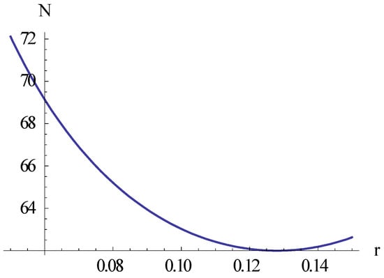
Figure 10.
The number of e-folds N as given in Equation (6.33.37) plotted as function of r.
We see that N has a minimum for with , so this model is marginally in agreement with the Planck data.
6.33.5. Tachyon Inflation with Constant Value of
Fei et al. also considered a tachyon inflation model with constant potential slow motion parameter . Integrating Equation (6.33.31) then gives
Inserting this into Equation (4.13) gives
Hence
With a positive value of requires . Inserting the expression (6.33.49) into the second of expressions (6.33.51) leads to
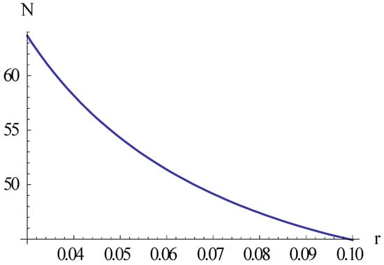
Figure 11.
The number of e-folds N as given in Equation (6.33.53) plotted as function of r.
We see that in order to have the tensor to scalar ratio must obey which is marginally in agreement with the Planck data.
Inserting the expression (6.33.51) for r into Equation (3.55) and integrating gives
where .
6.33.6. Self-Dual Tachyon Inflation
D. A. Steer and F. Vernizzi, [28] and also Rezazadeh, Karami and Hashemi [173] have considered a tachyon inflation model with the same potential (6.8.1) as in the S-dual model and used the horizon-flow parameters to calculate the scalar spectral index, its running and the tensor to scalar ratio. The potential is written
where and . The tachyon field has approximately the field strength during the inflationary era. From Equation (6.33.22) we then get
Inserting these expressions into those in Equation (4.56), we obtain
These expressions are different from those in Equation (6.8.6) for the same potential in standard single field inflation. It follows from the expressions for and that
Inserting the BPK-values and , corresponding to , gives . Furthermore
Hence showing that the running of the scalar spectral index is very small in this inflationary model.
Inserting the potential (6.33.55) into Equation (6.33.34) gives the number of e-folds
The end of the inflationary era takes place when , giving
To 2. order in this gives
Hence we can use the approximation in Equation (6.33.58), giving , which leads to
It follows that
Inserting these expressions into Equation (6.33.57) gives
6.33.7. Exponential Tachyon Inflation
Steer and F. Vernizzi, [28] and Rezazadeh, Karami and Hashemi [173] have also considered a tachyon inflation model with exponential potential
The corresponding model in standard inflation was considered in Section 4.4 and then leads to power law inflation as given in Equation (4.4.7), and a tensor-to-scalar ratio that is larger than allowed by the Planck data. However in the Tachyon inflation scenario the model with this potential give more interesting predictions, as will be shown below.
Inserting the potential (6.33.66) into Equation (6.33.15) and integrating with gives the time dependency of the tachyon potential
where is a positive constant. The potential has a power law time dependence
Hence, according to the slow roll approximation (6.33.12) the Hubble parameter is.
The first Hubble slow roll parameter, given in Equation (6.33.11), is
The slow roll era ends when giving
Inserting the potential (6.33.66) into Equation (6.33.38) and performing the integration gives
The last three equations together with Equation (6.33.22) give
Inserting this into Equation (4.56) we
Inserting gives in good agreement with the inflationary requirements. The expressions (6.33.71) imply which is too large to be compatible with the Planck data. Furthermore . Note the agreement with the tachyonic inflation with exponential inflation and the prediction (6.1.37) of standard inflation with power law inflation having —the so-called chaotic inflation.
6.33.8. Inverse Power Law Tachyon Inflation
Rezazadeh, Karami and Hashemi [173] have also considered tachyon inflation with inverse power-law potential,
Inserting this into Equation (6.33.13) and integrating with and gives
Hence
Inserting this into Equation (6.33.4) and neglecting compared to 1 in the slow roll era, we get
Normalizing the scale factor to gives
It follows from Equations (6.33.15) and (6.33.75) that the first Hubble slow roll parameter is
For the slow roll parameter is constant, and then there is no graceful exit from the slow roll era. Furthermore Rezazadeh, Karami and Hashemi [173] have shown that this model is ruled out by the Planck data. The inflaton field increases with time for . A graceful exit of the slow roll era requires that increases with time and hence that .
Inserting the potential (6.33.73) into Equation (6.33.41) and performing the integration gives
The slow roll era ends when , giving
Hence
Inserting this into Equation (6.33.80) gives
From Equation (6.33.28) we now obtain
These expressions imply that
With this relationship gives while the BPK-data require , so this model is not in agreement with the observational data.
6.33.9. Tachyon-Intermediate Inflation
S. del Campo, R. Herrera and A. Toloza [203] have considered the intermediate inflation in the tachyonic framework. Then the scale factor is given in Equation (6.30.1). The Hubble parameter and its derivatives with respect to cosmic time are given in Equation (6.30.2). However Equation (2.1) is now replaced by (6.33.1) so the density and pressure of the tachyonic field are not given by Equation (6.30.3).
Inserting the expressions (6.30.2) into Equation (6.33.6) and integrating with gives
which replaced Equation (5.30.5) in the ordinary intermediate inflation. It is assumed that . Hence the tachyon field is an increasing function of time. From Equations (6.33.4) and (6.33.6) we obtain
Inserting the expressions (6.30.2) gives
It follows from Equations (6.33.84) and (6.33.86) that the potential as a function of the tachyon field is
The Hubble slow roll parameters are given as a function of time in Equation (6.30.9). Combining this with Equation (6.33.88) leads to
Hence is a decreasing function of time. So like standard intermediate inflation there is no natural finish of the slow roll era, and the parameter is used to define the initial value of the inflaton field by the condition , giving
When combining Equations (6.30.11) and (6.33.84) we find that the number of e-folds during the inflationary era is
The tachyon inflaton potential is an increasing function of N. Inserting this into Equation (6.33.91) gives
Hence
In tachyon inflation, the scalar spectral index is not given in the same way as in standard inflation in terms of the Hubble parameters. However, Rezazadeh et al. [173] have shown that the relation is
It follows from this relationship that . Hence these inflationary models are ruled out by the BPK-data which according to Gott and Colley [46], require .
6.33.10. The N-Formalism Applied to Tachyon Inflation
N. Barbosa-Cendejas et al. [61,201] have used the N-formalism and the horizon-flow parameters, and studied a tachyon inflationary model with of the perturbative class considered in Section 5.2. Then Equation (3.73) takes the form
Inserting this into Equation (6.33.94) and performing the integration gives
Substituting this into Equation (6.33.33) and integrating with shows that the potential is
From Equations (6.33.97) and (6.33.25) we get
This gives
When comparing with Equation (6.1.44) we see that the last of these equations is the same consistency relationship as that for ordinary polynomial inflation. With we get . This value of the tensor-to-scalar ratio is larger than allowed by the most recent analysis of the observational data [46], .
Fei et al. [75] have considered a model with
Inserting this into Equation (6.33.26) gives
The solution of this equation with is
where and are constants. Inserting this into Equation (6.20.32) gives
The constants are determined by the condition that the slow roll era ends when , giving
Hence the potential and the first horizontal slow roll parameter are
and
Combining this with Equation (6.33.107) we get the relations
The tensor-to-scalar ratio r is plotted as function of A from the expression (6.33.109) for with and in Figure 12.
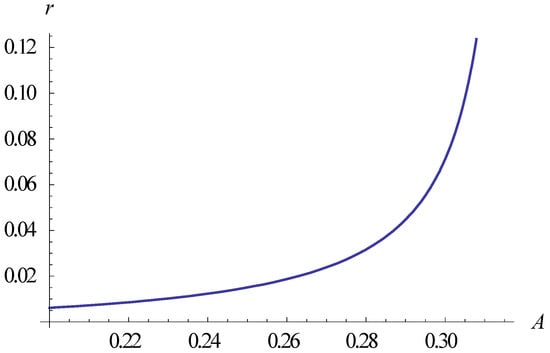
Figure 12.
The tensor to scalar ratio as given in Equation (6.33.111) for plotted as function of A in the region for and .
The factor changes sign for
Inserting and gives while gives . Because is so large, r changes sign close to . Since only positive values of r are allowed, this class of models require that . This is the reason of the restricted range of A in Figure 12.
It may be noted that
With gives .
Equation (6.33.103) can be written as
Hence requires . Inserting gives . The value gives . With we have . However negative values of A are not allowed by the expression (6.33.109) for . So the model with is excluded by the Planck data.
The relationship between the tachyon inflaton potential and the number of e-folds of the scale factor during the slow roll era can be calculated by inserting Equation (6.33.107) into Equation (6.33.35). Performing the integration with one obtains for ,
Inserting this into Equation (6.33.107) one obtains the inverse power law potential
In the special case with and the potential takes the form
For the potential as given in Equation (6.33.107) takes the form
Inserting this equation into Equation (6.33.32) and integrating with gives
Substituting this into Equation (6.33.116) gives
The expression reduces to the exponential potential
if . In this case Equation (6.33.102) gives which is an acceptable value of N. Inserting these values into the first expression in Equation (6.33.109) gives . Hence the tachyonic inflationary model with an exponential potential is allowed by the observational data, while in the standard inflationary scenario the model with exponential potential gives too high value of r as seen in Equation (6.4.12).
Fei et al. [75] have also considered a class of tachyonic inflationary models with the first horizontal slow roll parameter given by
where I have used the notation of Equation (5.66). The -relationship is the same as Equation (5.67) in the standard inflationary scenario, and a prediction of this class of inflationary models is that . However, the expressions of the potential are different in the tachyonic inflationary scenario.
We can use the Planck data to estimate realistic values of p and . The scalar tilt and the tensor-to-scalar ratio are
From these equations it follows that the -relation has the form
We can now express p and in terms of and N as
Inserting , solving the first equation numerically for p, and inserting the result into the second equation, gives . Hence these are realistic values for this class of tachyonic inflationary models.
Substituting Equation (6.33.120) into Equation (6.33.27) and integrating gives
It was shown by Fei et al. [75] that the potential cannot be expressed by T in terms of elementary functions for arbitrary values of p. We therefore proceed with the case . In this case
Inserting gives and which is too large in relation to the Planck data.
Inserting the expression of the potential for in Equation (6.33.124) into Equation (6.33.32) and integrating with gives
Combining Equations (6.33.124) and (6.33.126) gives the potentials
Let us consider an inverse power law potential of the form
Steer and Vernizzi [28] considered the special case with . Inserting Equation (6.33.128) into Equation (6.33.20), the horizon slow roll parameters are found to be
Furthermore Steer and Vernizzi have assumed that and . Hence we have to leading order
Inflation ends when which gives
It follows from Equations (6.33.35) and (6.33.128) that the number of e-folds is
The two last equations give
Inserting this into Equation (6.33.130) and using that gives
Inserting these expressions into Equation (6.33.25) gives
The case was considered by Steer and Vernizzi. It gives
Hence we get the relationships
Inserting the Planck value gives and . Due to the large value of r this model is ruled out by the Planck data.
It follows from the expressions (6.33.135) that
The first of these equations can be written
Inserting this into the second of the Equation (4.33.135) gives
In order that p shall be positive we must have . With this gives while the Planck data favor . Hence the Planck data favor negative values of p because positive values give too large tensor-to-scalar ratio. Another way of seeing that the Planck data favor negative values of p is to solve the first of the Equation (6.20.131) with respect to p. This gives
Inserting gives . Substituting this into Equation (6.33.136) gives . A smaller value of r is favored, for example From Equation (6.33.139) we then get . Solving Equation (6.33.141) with respect to N gives
Putting into this equation gives which is too small. In Figure 13 we have plotted p as given in Equation (6.20.137) as a function of N for .
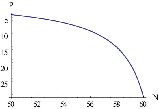
Figure 13.
The parameter p plotted as a function of N as given in Equation (6.33.136) for .
We see that the preferred values of p are .
Barbosa-Candejas et al. [201] considered a polynomial class of models with
Inserting the expression (6.33.143) into Equation (6.33.37) and performing the integration gives
From Equations (6.33.143), (6.33.144) and (6.33.24) we get
where . Hence the potential as a function of the tachyon field is
where .
Inserting the expression (6.33.143) into Equation (6.33.28) we obtain the spectral parameters for this class of inflationary models
This gives the -relationship
Inserting gives , which are acceptable values.
Barbosa-Candejas et al. [201] also investigated an exponential class of models with
Inserting the expression (6.33.149) into Equation (6.33.37) and integrating gives
From Equations (6.33.149), (6.33.150) and (6.33.24) we obtain
Hence the potential as a function of the inflaton field, is
Putting the expression (6.33.149) into Equation (6.33.28), we obtain the spectral parameters for this class of inflationary models
Hence the -relationship is
Inserting gives , which again are acceptable values.
Finally Barbosa-Candejas et al. [200] have studied the tachyonic version of S-dual inflation, with
Inserting the expression (6.33.155) into Equation (6.33.37) and integrating leads to
From Equations (6.33.155), (6.33.156), and (6.33.24) we obtain
Hence the potential as a function of the inflaton field, is
Inserting the expression (6.33.155) into Equation (6.33.28) we obtain the spectral parameters for this class of inflationary models
These expressions can be combined to give
Inserting gives in order to obtain agreement with the PBK-observations.
6.33.11. Tachyon Warm Intermediate Brane Inflation
V. Kamali, S. Basilakos and A. Mehrabi [204] have investigated tachyon warm-intermediate inflation in light of the Planck data. They have noted that while in cold standard tachyon inflation reheating is problematic because the tachyon fields in such models do not oscillate around the minimum of the potential, this problem can be alleviated in the context of warm inflation, where production of radiation occurs during the slow-roll era, which implies that reheating is not necessary.
For this class of models the density and pressure of the tachyon inflaton field is given by Equation (6.33.1). Inserting the expressions (6.33.1) into the brane version of the 1. Friedmann Equation (5.16.1), gives
The equations of continuity for the inflaton energy and the radiation energy are found in Equation (6.32.2). Inserting the expressions (6.33.1) into the equation of continuity of the tachyon field gives evolution equation of the tachyon field
Differentiating Equation (6.33.161), using that , and utilizing Equation (6.33.162) lead to
without any approximations. In the case of strong dissipation , and the equation reduces to
From Equation (6.33.161), we then get to lowest order in ,
It may be noted that Equation (13) of Kamali, Basilakos and Mehrabi is slightly different. They have for the last factor, but a series expansion gives the expression (6.33.165) to lowest order in .
Kamali, Basilakos and Mehrabi have investigated two cases, I. constant, and II. , where is the radiation temperature, and is a constant. With the number of e-folds they found for model I: , and for the model II: . Hence the models are in agreement with the Planck observational data.
6.33.12. Tachyon Natural Inflation
I shall here consider tachyon inflation with a potential like that of Equation (6.5.1)
This is the same as the potential in Equation (2) of Rashidi and Nozari [205]. We shall here put their warp factor . With this potential Equations (6.33.15) and (6.33.23) give
where . Note that Rashidi and Nozari have defined the slow roll parameters by the expressions (3.12) for and , (but without the factor 2 in the denominator in the expression for ,) and calculated the second slow roll parameter by using the first expression in Equation (6.33.23) for instead of the second one for .
The number of e-folds is found by inserting the potential (6.33.166) and its derivative into Equation (6.33.36), which gives
The final value of the tachyon fiel is given by which leads to
The scalar spectral tilt, the tensor-toscalar-ratio and the running of the scalar spectral index are given by (4.13) and (4.4), respectively. Inserting the expressions (6.33.167) and introducing a function by
leads to
Solving Equation (6.33.171) with respect to G gives
where the minus sign has been chosen due to the condition which leads to the requirement . With according to the Planck 2015 data, this demands that .
Inserting the expression (6.33.174) into Equation (6.33.172) gives the −relationship
The tensor-to-scalar-ratio r is plotted as a function of for in Figure 14.
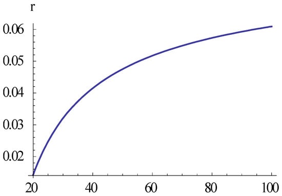
Figure 14.
Tensor to scalar ratio as function of β.
Here is an increasing function of with . Hence a prediction of this model is that or with .
7. Conclusions
The most recent analysis [46] (July 2017) of the combined Planck, BICEP2 and Keck results has given the restriction on the tensor-to-scalar-ratio for the CMB-radiation. This, together with the precise value of the scalar spectral index, , determined from the observations, rule out several classes of inflationary universe models. The observations are still not sufficiently accurate to give precise values of the other spectral parameters. Hence we shall here focus mostly upon the predicted relationship of different inflationary models in order to judge how well they come out of the confrontation with observational data.
- Polynomial inflation. The potential is given in Equation (6.1.1) and the relationship in (6.1.23). For and this relationship requires . Hence polynomial inflation with for example is ruled out by observations.
- Hilltop inflation. The potential is given in Equation (6.2.1). It was noted below Equation (6.2.12) that small field hilltop inflation is ruled out by the observational data. As shown in Equation (6.2.30) large field hilltop inflation predicts which is in agreement with observations. However in general large field inflation has an unsecure theoretical foundation since the energy scale of the symmetry breaking is larger than the Planck energy. Strictly speaking we need a quantum gravity theory to describe such models.
- Symmetry breaking inflation with potential (6.3.1). It was shown that this inflationary model predicts , or with the Planck data, . This is larger than the values, , favored by the BICEP2/Planck-Keck data, so this model is ruled out.
- Exponential potential inflation. For an inflation model with potential (6.4.1) the relationship is , which is in conflict with observations. However it is possible for models with the more general form (6.4.13) of the potential to be in agreement with observations.
- Natural inflation. The potentials are given in Equation (6.5.1). It was shown from the relationship (6.5.24) that the symmetry breaking mass is , i.e., much larger than the Planck mass in these models, which is somewhat problematic, since we are then outside the region of validity of the classical theory of relativity.
- Hybrid natural inflation with potential (6.6.1). It was shown that the hybrid natural inflation models are in trouble unless and .
- Higgs or Starobinsky inflation. The simplest form of the potential is given in Equation (6.7.2). This model predicts that which is in agreement with observations. The more general potential (6.7.13) gives the relationship . In general the Higgs-Starobinsky inflation models predict very small values of r. It should be noted, however, that there may exist a limit to how small r is allowed to be. Hamada and coworkers [206] have recently argued in the context of Higgs inflation, that the PandaX-II bound on the dark-matter mass, , leads to the requirement in most of the parameter space of elementary particle physics.
- S-dual inflation. These models have in general a potential of the form (6.8.2). It was shown that these models do not have a graceful exit of the slow roll era. Also they have an extra free parameter making exact predictions problematic.
- Hyperbolic inflation. The potential is given in Equation (6.9.1). These models are similar to those of the S-dual inflation, but they do not suffer from the exit problem. With suitable values of the two free parameters of these models they give values of the spectral parameters in accordance with observations.
- M-flation. The potential is given in Equation (6.10.1). This model predicts too large tensor-to-scalar ration and is ruled out by observations.
- Supergravity motivated inflation. These models have the potential (6.11.1) with two arbitrary parameters, that can be chosen so that a model in this class is in agreement with the observational data. There is also a so-called attractor model with a potential (6.11.9). This is in agreement with observations for .
- Goldstone inflation with potential (6.12.1). This model is mathematically identical to one of the natural inflation models and is a large field model. It can be adjusted to be in accordance with observations, but has the same foundational problems as natural inflation.
- Coleman-Weinberg inflation with potential (6.13.1). This class of models incorporates both small-fields and large-field models. The small field version is in agreement with observations, is physically well motivated, and is a promising inflation model.
- Kähler moduli inflation with potential (6.14.1). This model predicts a very small value of r and is in agreement with the present observational data.
- Hybrid inflation. Inflation models in this class have two fields, a so-called water-fall field and an inflaton field. The simplest version with potential (6.15.1) predicts too large value of r and is thus ruled out by the observational data.
- Brane inflation. The predicted tensor-to-scalar ratio for brane inflation with the polynomial potential (6.1.1) is given in Equation (6.16.29), which leads to the value . According to the most recent analysis of the observational data , so this brane model is ruled out by observations.
- Fast roll inflation with potential (6.17.1). This model predict . Hence it is ruled out by the observational data due to the high value it predicts for r.
- Running mass inflation with potential (16.18.1). This model has three free parameters, and hence it cannot predict the values of the optical parameters.
- K-inflation. Like fast roll inflation this class of models predict and is thus ruled out by the observational data.
- Dirac-Born-Infield inflation. A class of DBI-inflationary models with polynomial potential has been considered. According to Equation (6.20.2), it predicts , and is hence in conflict with observational data.
- Flux-brane inflation with potential (6.21.1). This model predicts giving for . This is lower than admitted in order to solve the horizon- and flatness problems.
- Mutated hilltop inflation with potential (6.22.1). This model is not ruled out by the Planck/BICEP2 observations.
- Arctan inflation with potential (6.23.1). In this model showing that the number of e-folds during the slow roll era is , which is a little less that the optimal number for solving the horizon and flatness problems.
- Inflation with fractional potential. One version of this model has potential (6.24.1). This leads to the prediction that for the tensor-to-scalar ratio is . Another version has potential (6.24.8) having a too small number of e-folds during the slow roll era to give a realistic inflationary scenario. A third version has potential (6.24.14) giving , which is close to being acceptable.
- Twisted inflation with potential (6.25.1). The tensor-to-scalar ratio has a very small value according to the twisted inflation model. It seems to be an acceptable inflation model.
- Inflation with invariant density spectrum. This model has potential (6.26.1) and has a scale invariant Harrison-Zeldovich density fluctuation spectrum. Also, the number of e-folds is less than one. Hence, this model is ruled out as a realistic inflationary model.
- Quintessential inflation. A first version has potential (6.27.6). This model of quintessential inflation predicts and is thus ruled out by observations. A second version has potential (6.27.8). Using it predicts and . This model is in agreement with observations. A third model has potential (6.27.14). With this model gives and in agreement with observations. A fourth model has potential (6.27.26) and turned out to be very unrealistic.
- Generalized Chaplygin gas inflation. The inflaton field has a potential given in Equation (6.28.13). With this model predicts . Since the number of e-folds is usually restricted to it is concluded that a universe dominated by generalized Chaplygin gas is not a suitable model of the inflationary era.
- Axion monodromy inflation with potential (6.29.1). With a reasonable value of a parameter in this model one obtains in agreement with the observational data.
- Intermediate inflation. The potential is given in Equation (6.30.8). The simplest versions of these models predict that , which is not allowed by observations.
- Constant rate of roll inflation. Maybe the most promising version of this class of models is the one with potential (6.31.45). However, the potential contains two arbitrary parameters, and this prevents a prediction of the tensor-to-scalar-ratio unless one can determine for example an initial condition defining the beginning of the slow roll era. Recently Yi and Gong [207] has shown that the model with potential (6.31.25) and is in conflict with the Planck data.
- Warm inflation. During the evolution of warm inflation dissipative effects are important, and inflaton field energy is transformed to radiation energy. This is a large class on inflationary models that may be realized in a large number of ways. In the warm inflation scenario a thermalized radiation component is present with temperature , where both T and H are expressed in units of energy. Then the tensor-to-scalar ratio is suppressed by the factor when compared with the standard cold inflation, where Q the so-called dissipative ratio defined in Equation (6.32.5).Let us summarize the predictions of some specific models.Warm polynomial inflation with an inflaton potential given by Equation (6.1.1) with has been investigated by Panotopoulos and Videla [182]. They found that in the weak dissipative regime when the scalar spectral tilt is , giving which is too small to be compatible with the standard inflationary scenario. However, in the strong dissipative regime when , the spectral parameters can be made to be in accordance with the observational data by choosing a proper value of an arbitrary parameter.Taylor and Berera [195] have briefly considered warm inflation models with an exponential potential, , and found that in the strong dissipation regime the scalar spectral index parameter for models of this type is negative in conflict with the Planck observations.Visinelli [189] has investigated warm natural inflation with potential (6.32.48). He found that this class of inflationary models predicts a vanishing value of the tensor-to-scalar-ratio.Several versions of warm viscous inflation have also been investigated, and their properties have been restricted in order to obtain agreement with the observational data. In all such models, the tensor-to-scalar-ratio has a small value, but without some fundamental theory making it possible to determine some physical parameters they cannot presdict the values of the CMB spectral parameters.
- Tachyon inflation. Tachyon inflation is a string theory inspired model of inflation. In these models it has become usual to introduce a so-called tachyon field, and denote it by T. The tachyon field is related to the usual inflaton field by Equation (6.33.16). Like warm inflation, this is a large class of inflationary models that may be realized in a large number of ways. Here, too, we shall summarize the predictions of some specific models.A class of models with , where is an arbitrary constant, leads to the relationship . With we get . This value of the tensor-to-scalar ratio is larger than allowed by the most recent analysis of the observational data [46], . This class of models have members with polynomial or exponential tachyon potentials.As shown in Figure 12, tachyon models with have when . Several other tachyon models may be made to agree with observations, but having more than one free parameter, that is not a prediction of the models, only adjustments after the observational results have been obtained.It has been shown that tachyon natural inflation predicts or with .It should also be mentioned that S. Chervon and coworkers [208,209,210] have developed a procedure for calculating the optical parameters of inflationary universe models exactly, without applying the slow roll approximation. One may show that the predictions made by means of such calculations deviate only a few per cent from those based upon the slow roll approximations.
In the present article I have given a systematic exposition of the dynamics of inflationary models, the three types of slow roll parameters—the potential-, the Hubble-, and the horizon-flow parameters-, and the N-formalism of inflationary models. Furthermore 33 classes of inflationary models have been described, many of them in a rather detailed way. Their predictions of the tensor-to-scalar-ratio has been calculated, given the measured scalar tilt, , and the proper range of the number of e-folds, , and compared to the requirement of the most recent analysis of the observational data. A supplementary review has been given in [211].
The main result is that many inflationary models can be ruled out because they predict to large value of r, and a few are strongly favored. Models that are ruled out by the observational data are: Most types of polynomial inflation, small field hilltop inflation, the main type of symmetry breaking inflation, the simples types of exponential potential inflation, some types of hybrid natural inflation, M-flation, the simplest types of hybrid inflation, brane inflation, fast roll inflation, K-inflation, Arctan-inflation, inflation with invariant density spectrum, two of the four models of quintessential inflation that were reviewed, generalized Chaplygin gas inflation, the simplest versions of intermediate inflation, and some types of tachyon inflation.
Other models are not attractive because they contain too may arbitrary parameters, implying that they have a rather phenomenological character and lack predictive force, or that their theoretical foundations are weak, such as for large field inflations that strictly speaking need a quantum gravity theory because their symmetry breaking energy is larger than the Planck energy, or they have no graceful exit of the slow roll era. Models in this category are: large field hilltop inflation, natural inflation, S-dual inflation, hyperbolic inflation, supergravity motivated inflation, Goldstone inflation, large field Coleman-Weinberg inflation and constant rate of roll inflation.
The models of inflation that come best out of the confrontation with observational data, have a graceful exit of the slow roll era, and are also able to predict a value for r given the restrictions mentioned above of and N are: Higgs or Starobinsky inflation, small field Coleman-Weinberg inflation, Kähler moduli inflation, standard DBI-inflation, mutated hilltop inflation, some versions of inflation with fractional potential, twisted inflation, some types of quintessential inflation, axion monodromy inflation, and many types of warm inflation.
In general, warm inflation seems to be the class with physically most realistic inflationary models, and also those that come best out of the confrontation with observational data.
Conflicts of Interest
The author declares no conflicts of interest.
References
- Ade, P.; Aghanim, N.; Armitage-Caplan, C.; Arnaud, M.; Ashdown, M.; Atrio-Barandela, F.; Aumont, J.; Baccigalupi, C.; Banday, A.J.; Barreiro, R.B.; et al. Planck 2013 results. XXX. Cosmic infrared background measurements and implications for star formation. Astron. Astrophys. 2014, 571, A30. [Google Scholar]
- Ade, P.; Aghanim, N.; Ahmed, Z.; Aikin, R.W.; Alexander, K.D.; Arnaud, M.; Aumont, J.; Baccigalupi, C.; Banday, A.J.; Barkats, D.; et al. Joint Analysis of BICEP2/Keck Array and Planck Data. Phys. Rev. Lett. 2015, 114, 101301. [Google Scholar] [CrossRef] [PubMed]
- Watson, G.S. An Exposition on Inflationary Cosmology. arXiv, 2000; arXiv:astro-ph/0005003. [Google Scholar]
- Linde, A.D. Inflationary Cosmology. Lect. Notes Phys. 2008, 738, 1–54. [Google Scholar]
- Kinney, W.H. Cosmology, inflation, and the physics of nothing. In Techniques and Concepts of High-Energy Physics XII; NATO Science Series; Springer: Berlin, Germany, 2003; Volume 123, pp. 189–243. [Google Scholar]
- Ade, P.; Aghanim, N.; Armitage-Caplan, C.; Arnaud, M.; Ashdown, M.; Atrio-Barandela, F.; Aumont, J.; Baccigalupi, C.; Banday, A.J.; Barreiro, R.B.; et al. Planck 2013 results. XVI. Cosmological parameters. Astron. Astrophys. 2014, 571, A16. [Google Scholar]
- Ade, P.; Aghanim, N.; Armitage-Caplan, C.; Arnaud, M.; Ashdown, M.; Atrio-Barandela, F.; Aumont, J.; Baccigalupi, C.; Banday, A.J.; Barreiro, R.B.; et al. Planck 2013 results. XXII. Constraints on inflation. Astron. Astrophys. 2014, 571, A22. [Google Scholar]
- Germán, G.; Herrera-Aguilar, A.; Hidalgo, J.C.; Sussman, R.A. Canonical single field slow-roll inflation with a non-monotonic tensor-to-scalar ratio. J. Cosmol. Astropart. Phys. 2016, 2016, 025. [Google Scholar] [CrossRef]
- Liddle, A.R.; Parsons, P.; Barrow, J.D. Formalizing the slow roll approximation in inflation. Phys. Rev. D 1994, 50, 7222–7232. [Google Scholar] [CrossRef]
- Peiris, H.V.; Komatsu, E.; Verde, L.; Spergel, D.N.; Bennett, C.L.; Halpern, M.; Hinshaw, G.; Jarosik, N.; Kogut, A.; Limon, M.; et al. First-year Microwave Anisotropy Probe (WMAP) Observations: Implications for Inflation. Astrophys. J. Suppl. 2003, 148, 213–231. [Google Scholar] [CrossRef]
- Schwarz, D.J.; Terrero-Escalante, C.A. Primordial fluctuations and cosmological inflation after WMAP1. J. Cosmol. Astropart. Phys. 2004, 2004, 003. [Google Scholar] [CrossRef]
- Creminelli, P.; Nacir, D.L.; Simonović, M.; Trevisan, G.; Zaldarriaga, M. Φ2 Inflation at its Endpoint. Phys. Rev. D 2014, 90, 083513. [Google Scholar] [CrossRef]
- Correia, F.P.; Schmidt, M.G.; Tavartkiladze, Z. Natural Inflation from 5D SUGRA and Low Reheat Temperature. Nucl. Phys. B 2015, 898, 173–196. [Google Scholar] [CrossRef]
- Kinney, W.H. Inflation: Flow, fixed points and observables to arbitrary order in slow roll. Phys. Rev. D 2002, 66, 083508. [Google Scholar] [CrossRef]
- Kolb, E.W. A coasting cosmology. Astrophys. J. 1989, 344, 543–550. [Google Scholar] [CrossRef]
- Turok, N. Global Texture as the Origin of Cosmic Structure. Phys. Rev. Lett. 1989, 63, 2625–2628. [Google Scholar] [CrossRef] [PubMed]
- Grøn, Ø.; Johannesen, S. Conformally flat spherically symmetric spacetimes. Eur. Phys. J. Plus 2013, 128, 92. [Google Scholar] [CrossRef]
- Leach, S.M.; Liddle, A.R.; Martin, J.; Schwarz, D.J. Cosmological parameter estimation and the inflationary cosmology. Phys. Rev. D 2002, 66, 023515. [Google Scholar] [CrossRef]
- Martin, J. The Observational Status of Cosmic Inflation After Planck. In The Cosmic Microwave Background; Fabris, J., Piattella, O., Rodrigues, D., Velten, H., Zimdahl, W., Eds.; Astrophysics and Space Science Proceedings; Springer: Cham, Switzerland, 2016; Volume 45. [Google Scholar]
- Spaliński, M. New Solutions of the Inflationary flow equations. J. Cosmol. Astropart. Phys. 2007, 2007, 016. [Google Scholar] [CrossRef]
- Lyth, D.H. What would we learn by detecting a gravitational wave signal in the cosmic microwave background anisotropy? Phys. Rev. Lett. 1997, 78, 1861–1863. [Google Scholar] [CrossRef]
- Lyth, D.H.; Riotto, A. Particle Physics Models of Inflation and Cosmological Density Perturbation. Phys. Rep. 1999, 314, 1–146. [Google Scholar] [CrossRef]
- Easther, R.; Kinney, W.H.; Powell, B.A. The Lyth Bound and the End of Inflation. J. Cosmol. Astropart. Phys. 2006, 2006, 004. [Google Scholar] [CrossRef]
- Germán, G. On the Lyth bound and single-field slow roll inflation. arXiv, 2014; arXiv:1405.3246. [Google Scholar]
- Coone, D.; Roest, D.; Vennin, V. The Hubble flow of Plateau Inflation. J. Cosmol. Astropart. Phys. 2015, 2015, 010. [Google Scholar] [CrossRef]
- Vennin, V. Horizon-Flow off-track for Inflation. Phys. Rev. D 2014, 89, 083526. [Google Scholar] [CrossRef]
- Martin, J.; Ringeval, C.; Vennin, V. Encyclopædia Inflationaris. Phys. Dark Univ. 2014, 5–6, 75–235. [Google Scholar] [CrossRef]
- Steer, D.A.; Vernizzi, F. Tachyon inflation: Tests and comparison with single scalar field inflation. Phys. Rev. D 2004, 70, 043527. [Google Scholar] [CrossRef]
- Myrzakulov, R.; Sebastiani, L.; Zerbini, S. Reconstruction of Inflation Models. Eur. Phys. J. C 2015, 75, 215. [Google Scholar] [CrossRef]
- Mukhanov, V. Quantum Cosmological Perturbations: Predictions and Observations. Eur. Phys. J. C 2013, 73, 2486. [Google Scholar] [CrossRef]
- Ballesteros, G.; Casas, J.A. Large tensor-to-scalar ratio and running of the scalar spectral index with instep inflation. Phys. Rev. D 2015, 91, 043502. [Google Scholar] [CrossRef]
- Kinney, W.H. Horizon crossing and inflation with large η. Phys. Rev. D 2005, 72, 023515. [Google Scholar] [CrossRef]
- Martin, J.; Motohashi, H.; Suyama, T. Ultra Slow-Roll Inflation and the non-Gaussianity Consistency Relation. Phys. Rev. D 2013, 87, 023514. [Google Scholar] [CrossRef]
- Dimopoulos, K. Slow-roll versus ultra slow-roll inflation. Phys. Lett. B 2017, 775, 262–265. [Google Scholar] [CrossRef]
- Ade, P. Planck 2015 results. XX. Cosmological parameters. Astron. Astrophys. 2016, 594, A13. [Google Scholar]
- Ade, P. Planck 2015 results. XIII. Constraints on inflation. Astron. Astrophys. 2016, 594, A20. [Google Scholar]
- Huang, Q. Lyth bound revisited. Phys. Rev. D 2015, 91, 123532. [Google Scholar] [CrossRef]
- Baumann, D. TASI Lectures on Inflation. arXiv, 2012; arXiv:0907.5424. [Google Scholar]
- Ade, P.; Aikin, R.W.; Barkats, D.; Benton, S.J.; Bischoff, C.A.; Bock, J.J.; Brevik, J.A.; Buder, I.; Bullock, E.; Dowell, C.D.; et al. BICEP 2 I: Detection of B-mode Polarization at Degree Angular scales. Phys. Rev. Lett. 2014, 112, 241101. [Google Scholar] [CrossRef] [PubMed]
- Ashoorioon, A.; Dimopoulos, K.; Sheikh-Jabbari, M.M.; Shiu, G. Non-Bunch-Davis Initial State Reconciles Chaotic Models with BICEP and Planck. Phys. Lett. B 2014, 737, 98–102. [Google Scholar] [CrossRef]
- Gao, Q.; Gong, Y.; Li, T. The Modified Lyth Bound and Implications of BICEP2 Results. Phys. Rev. D 2015, 92, 063509. [Google Scholar] [CrossRef]
- Gao, Q.; Gong, Y. The challenge for the single field inflation with BICEP2 result. Phys. Lett. B 2014, 734, 41–43. [Google Scholar] [CrossRef]
- Gao, X.; Li, T.; Shukla, P. Fractional-chaotic inflation in the lights of PLANCK and BICEP2. Phys. Lett. B 2014, 738, 412–417. [Google Scholar] [CrossRef]
- Benetti, M.; Ramos, R.O. Warm dissipative effects predictions and constraints from the Planck data. Phys. Rev. D 2017, 95, 023517. [Google Scholar] [CrossRef]
- Bamba, K.; Odintsov, S.; Saridakis, E.N. Inflationary Cosmology in unimodular F(T) gravity. Mod. Phys. Lett. A 2017, 32, 1750114. [Google Scholar] [CrossRef]
- Gott III, J.R.; Colley, W.N. Reanalysis of the BICEP2, Keck and Planck Data: No Evidence for Gravitational Radiation. arXiv, 2017; arXiv:1707.06755. [Google Scholar]
- Minor, K.E.; Kaplinghat, M. Inflation that runs naturally, gravitational waves and suppression of power at large and small scales. Phys. Rev. D 2014, 91, 063504. [Google Scholar] [CrossRef]
- Antusch, S.; Nolde, D. BICEP2 implications for single field slow-roll inflation revisited. J. Cosmol. Astropart. Phys. 2014, 2014, 035. [Google Scholar] [CrossRef]
- Bramante, J.; Lehman, L.; Martin, A. Clearing the Brush: The Last Stand of Solo Small Field Inflation. Phys. Rev. D 2014, 90, 023530. [Google Scholar] [CrossRef]
- Barenboim, G.; Park, Wan-Il. On the tensor-to-scalar ratio in large single-field inflation models. arXiv, 2015; arXiv:1509.07132. [Google Scholar]
- Huang, Q.; Wang, S. No evidence for the blue-tilted power spectrum of relic gravitational waves. J. Cosmol. Astropart. Phys. 2015, 2015, 021. [Google Scholar] [CrossRef]
- Stewart, E.D.; Lyth, D.H. A more accurate analytic calculation of the spectrum of cosmological perturbations produced during inflation. Phys. Lett. B 1993, 302, 171–175. [Google Scholar] [CrossRef]
- Huang, Q. Slow roll reconstruction for running spectral index. Phys. Rev. D 2007, 76, 043505. [Google Scholar] [CrossRef]
- Vallinotto, A.; Copeland, E.J.; Kolb, E.W.; Liddle, A.R.; Steer, D.A. Inflationary potentials yelding constant scalar perturbation spectral indices. Phys. Rev. D 2004, 69, 103519. [Google Scholar] [CrossRef]
- Hodges, H.; Blumenthal, G. Arbitrariness of inflationary fluctuation spectra. Phys. Rev. D 1990, 42, 3329. [Google Scholar] [CrossRef]
- Amoros, J.; de Haro, J. The twilight of the single slow rolling inflation. arXiv, 2015; arXiv:1503.02153. [Google Scholar]
- Czerny, M.; Kobayashy, T.; Takahashi, F. Running Spectral Index from Large-field Inflation with modulations Revisited. Phys. Lett. B 2014, 735, 176–180. [Google Scholar] [CrossRef]
- Carrillo-González, M.; German, G.; Herrera-Aguilar, A.; Hidalgo, J.C.; Sussman, R. Testing hybrid natural inflation with BICEP2. Phys. Lett. B 2014, 734, 345–349. [Google Scholar] [CrossRef]
- Cheng, C.; Huang, Q.G. The Tilt of Primordial Gravitational WavesSpectra from BICEP2. Mod. Phys. Lett. A 2014, 29, 1450185. [Google Scholar]
- Cheng, C.; Huang, Q.G. Constraints on the cosmological parameters from BICEP2, Planck and WMAP. Eur. Phys. J. C 2014, 74, 3139. [Google Scholar] [CrossRef]
- Barbosa-Cendejas, N.; De-Santiagoa, J.; Germana, G.; Hidalgoa, J.C.; Mora-Lunaa, R.R. Tachyon inflation in the N-formalism. J. Cosmol. Astropart. Phys. 2015, 2015, 020. [Google Scholar] [CrossRef]
- Engqvist, K.; Mazumdar, A.; Stephens, P. Inflection point inflation within supersymmetry. J. Cosmol. Astropart. Phys. 2010, 2010, 020. [Google Scholar] [CrossRef]
- Choi, S.-M.; Lee, H.M. Inflection point inflation and reheating. Eur. Phys. J. C 2016, 76, 303. [Google Scholar] [CrossRef]
- Okada, N.; Okada, S.; Raut, D. Inflection-point inflation in hyper-charge oriented U(1)X model. Phys. Rev. D 2017, 95, 055030. [Google Scholar] [CrossRef]
- Bamba, K.; Nojiri, S.; Odintsov, S.D. Reconstruction of scalar field theories realizing inflation consistent with the Planck and BICEP2 results. Phys. Lett. B 2014, 737, 374–378. [Google Scholar] [CrossRef]
- Garcia-Bellido, J.; Roest, D. The large-N running of the spectral index of inflation. Phys. Rev. D 2014, 89, 103527. [Google Scholar] [CrossRef]
- Garcia-Bellido, J.; Roest, D.; Scalisi, M.; Zavala, I. The Lyth Bound of Inflation with a Tilt. Phys. Rev. D 2014, 90, 123539. [Google Scholar] [CrossRef]
- Bamba, K.; Odintsov, S.D. Inflation in a viscous fluid model. Eur. Phys. J. C 2016, 76, 18. [Google Scholar] [CrossRef]
- Chiba, T. Reconstructing the inflaton potential from the spectral index. Progr. Theor. Exp. Phys. 2015, 2015, 073E02. [Google Scholar] [CrossRef]
- Roest, D. Universality classes of inflation. J. Cosmol. Astropart. Phys. 2014, 2014, 007. [Google Scholar] [CrossRef]
- Mukhanov, V. Inflation without selfreproduction. Prog. Phys. 2014, 63, 36–41. [Google Scholar] [CrossRef]
- Lin, J.; Gao, Q.; Gong, Y. The reconstruction of inflationary potentials. Mon. Not. R. Astron. Soc. 2016, 459, 4029–4037. [Google Scholar] [CrossRef]
- Barranko, L.; Boubekeur, L.; Mena, O. A model-independent fit to Planck and BICEP2 data. Phys. Rev. D 2014, 90, 063007. [Google Scholar] [CrossRef]
- Gao, Q.; Gong, Y. Reconstruction of extended inflationary potentials for attractors. arXiv, 2017; arXiv:1703.02220. [Google Scholar]
- Fei, Q.; Gong, Y.; Lin, J.; Yi, Z. The reconstruction of Tachyon inflationary potentials. J. Cosmol. Astropart. Phys. 2017, 2017, 018. [Google Scholar] [CrossRef]
- Creminelli, P.; Dubovsky, S.; Nacir, D.L.; Simonović, M.; Trevisan, G.; Villadoro, G.; Zaldarriaga, M. Implications of the scalar tilt for the tensor-to-scalar ratio. Phys. Rev. D 2015, 92, 123528. [Google Scholar] [CrossRef]
- Gobetti, R.; Pajer, E.; Roest, D. On the Three Primordial Numbers. J. Cosmol. Astropart. Phys. 2015, 2015, 058. [Google Scholar] [CrossRef]
- Koh, S.; Lee, B.H.; Tumurtushaa, G. Reconstruction of the Scalar Field Potential in Inflationary Models with a Gauss-Bonnet term. Phys. Rev. D 2017, 95, 123509. [Google Scholar] [CrossRef]
- Kallosh, R.; Linde, A. Universality Class in Conformal Inflation. J. Cosmol. Astropart. Phys. 2013, 2013, 002. [Google Scholar] [CrossRef]
- Davis, J.L.; Levi, T.S.; Van Raamsdonk, M.; Whyte, K.R.L. Twisted Inflation. J. Cosmol. Astropart. Phys. 2010, 2010, 032. [Google Scholar] [CrossRef]
- Biagetti, M.; Kehagias, A.; Riotto, A. What We Can Learn from the Running of the Spectral Index if no Tensors are Detected in the Cosmic Microwave Background Anisotropy. Phys. Rev. D 2015, 91, 103527. [Google Scholar] [CrossRef]
- Binétruy, P.; Kiritsis, E.; Mabillard, J.; Pieroni, M.; Rosset, C. Universality classes for models of inflation. J. Cosmol. Astropart. Phys. 2015, 2015, 033. [Google Scholar] [CrossRef]
- Linde, A.D. Inflationary Cosmology after Planck 2013. arXiv, 2014; arXiv:1402.0526. [Google Scholar]
- Linde, A.D. Chaotic Inflation. Phys. Lett. B 1983, 129, 177–181. [Google Scholar] [CrossRef]
- Clesse, S. An introduction to inflation after Planck: From theory to observations. arXiv, 2015; arXiv:1501.00460. [Google Scholar]
- Barrow, J.D.; Liddle, J.D. Perturbation spectra from intermediate inflation. Phys. Rev. D 1993, 47, R5219–R5223. [Google Scholar] [CrossRef]
- Rezazadeh, K.; Karami, K.; Hashemi, S. Tachyon inflation with steep potentials. Phys. Rev. D 2017, 95, 103506. [Google Scholar] [CrossRef]
- Kinney, W.H.; Kolb, E.W.; Melchiorri, A.; Riotto, A. Inflation model constraints from the Wilkinson Anisotropy Probe three-year data. Phys. Rev. D 2006, 74, 023502. [Google Scholar] [CrossRef]
- Chiba, T.; Kohri, K. Consistency Relations for Large Field Inflation. Prog. Theor. Exp. Phys. 2014, 2014, 093E01. [Google Scholar] [CrossRef]
- Kobayashi, T.; Seto, O. Polynomial inflation models after BICEP2. Phys. Rev. D 2014, 89, 103524. [Google Scholar] [CrossRef]
- Destri, C.; de Vega, H.J.; Sanchez, N.G. MCMC analysis of WMAP3 and SDSS data points to broken symmetry inflation potentials and provides a lower bound on the tensor to scalar ratio. Phys. Rev. D 2008, 77, 043509. [Google Scholar] [CrossRef]
- de Haro, J.; Amorós, J.; Pan, S. Simple inflationary quintessential model. Phys. Rev. D 2016, 93, 084018. [Google Scholar] [CrossRef]
- Boubekeur, L.; Lyth, D.H. Hilltop Inflation. J. Cosmol. Astropart. Phys. 2005, 2005, 010. [Google Scholar] [CrossRef]
- Kohri, K.; Lin, C.M.; Lyth, D.H. More hilltop inflation models. J. Cosmol. Astropart. Phys. 2007, 2007, 004. [Google Scholar] [CrossRef]
- Basilakos, S.; Lima, J.A.S.; Solà, J. A viable Starobinsky-like inflationary scenario in the light of Planck and BICEP2 results. Int. J. Mod. Phys. D 2014, 23, 1442011. [Google Scholar] [CrossRef]
- Kinney, W.H.; Mahanthappa, K.T. Inflation at Low Scales: General Analysis and a Detailed Model. Phys. Rev. D 1996, 53, 5455–5467. [Google Scholar] [CrossRef]
- Zarei, M. On the running of the spectral index to all orders: A new approach to constraint the inflationary models. Class. Quantum Gravity 2016, 33, 115008. [Google Scholar] [CrossRef]
- Lyth, D.H.; Liddle, A.R. The Primordial Density Perturbation; Cambridge University Press: Cambridge, UK, 2009. [Google Scholar]
- Pieroni, M. Classification of Inflationary Models and Constraints on Fundamental Physics. Ph.D. Thesis, Paris Diderot University, Paris, France, 2016. [Google Scholar]
- Shiu, G.; Henry Tye, S.H. Some aspects of brane inflation. Phys. Lett. B 2001, 516, 421–430. [Google Scholar] [CrossRef]
- Drees, M.; Erfani, E. Running Spectral Index and Formation of Primordial Black Hole in Single Field Inflation Models. J. Cosmol. Astropart. Phys. 2012, 2012, 035. [Google Scholar] [CrossRef]
- Lu, Z. Inflation in the Generalized Inverse Power Law Scenario. J. Cosmol. Astropart. Phys. 2013, 2013, 038. [Google Scholar] [CrossRef]
- Chung, Y.; Lin, E. Topological inflation with large tensor-to-scalar-ratio. J. Cosmol. Astropart. Phys. 2014, 2014, 020. [Google Scholar] [CrossRef]
- Escudero, M.; Ramírez, H.; Boubekeur, L.; Giusarma, E.; Mena, O. The present and future of the most favored inflationary models after Planck 2015. J. Cosmol. Astropart. Phys. 2016, 2016, 020. [Google Scholar] [CrossRef]
- Rehman, M.U.; Shafi, Q.; Wickman, J.R. GUT Inflation and Proton Decay after WMAP 5. Phys. Rev. D 2008, 78, 123516. [Google Scholar] [CrossRef]
- Liddle, R.A. Power-law inflation with exponential potentials. Phys. Lett. B 1989, 4, 502–508. [Google Scholar] [CrossRef]
- Motohashi, H.; Starobinsky, A.A.; Yokoyama, J. Inflation with a constant rate of roll. J. Cosmol. Astropart. Phys. 2015, 2015, 018. [Google Scholar] [CrossRef]
- Lucchin, F.; Matarrese, S. Power-law Inflation. Phys. Rev. D 1985, 32, 1316. [Google Scholar] [CrossRef]
- Story, K.T.; Reichardt, C.L.; Hou, Z.; Keisler, R.; Aird, K.A.; Benson, B.A.; Bleem, L.E.; Carlstrom, J.E.; Chang, C.L.; Cho, H.; et al. A measurement of the cosmic microwave background damping tail from the 2500-square-degree SPT-Sz survey. Astrophys. J. 2013, 779, 86. [Google Scholar] [CrossRef]
- Unnikrishnan, U.; Sahni, V. Resurrecting power law inflation in the light of Planck results. J. Cosmol. Astropart. Phys. 2013, 2013, 063. [Google Scholar] [CrossRef]
- Geng, C.Q.; Hossain, W.; Myrzakulov, R.; Sami, M.; Saridakis, E.N. Quintessential inflation with canonical and noncanonical scalar fields and Planck 2015 results. Phys. Rev. D 2015, 92, 023522. [Google Scholar] [CrossRef]
- Alcaniz, J.S.; Carvalho, F.C. β-exponential inflation. Europhys. Lett. Assoc. 2006, 79, 39001. [Google Scholar] [CrossRef]
- Santos, M.A.; Menetti, M.; Alcanis, J.; Brito, F.A.; Silva, R. CMB constraints on β-exponential inflationary models. arXiv, 2017; arXiv:1710.09808. [Google Scholar]
- Freese, K.; Frieman, J.A.; Olinto, A.V. Natural inflation with pseudo Nambu-Goldstone bosons. Phys. Rev. Lett. 1990, 65, 3233. [Google Scholar] [CrossRef] [PubMed]
- Freese, K.; Kinney, W.H. On Natural Inflation. Phys. Rev. D 2004, 70, 083512. [Google Scholar]
- Freese, K.; Kinney, W.H. Natural Inflation: Consistency with Cosmic Microwave Background Observations of Planck and BICEP 2. J. Cosmol. Astropart. Phys. 2015, 2015, 044. [Google Scholar] [CrossRef]
- Kohri, K.; Lim, C.S.; Lin, C.M. Distinguishing between Extra Natural Inflation and Natural Inflation after BICEP2. J. Cosmol. Astropart. Phys. 2014, 2014, 001. [Google Scholar] [CrossRef]
- Márián, I.G.; Defenu, N.; Trombettoni, A.; Nándori, I. Pseudo Periodic Higgs Inflation. arXiv, 2017; arXiv:1705.10276. [Google Scholar]
- Ross, G.G.; Germán, G. Hybrid natural inflation from non Abelian discrete symmetry. Phys. Lett. B 2010, 684, 199–204. [Google Scholar] [CrossRef]
- Hebecker, A.; Kraus, S.C.; Westphal, A. Evading the Lyth bound in Hybrid Natural Inflation. Phys. Rev. D 2013, 88, 123506. [Google Scholar] [CrossRef]
- Vázquez, J.A.; Carrillo-González, M.; Germán, G.; Herrera-Aguilar, A.; Hidalgo, J.C. Constraining Hybrid Natural Inflation with recent CMB data. J. Cosmol. Astropart. Phys. 2015, 2015, 039. [Google Scholar] [CrossRef]
- Ross, G.G.; Germán, G.; Vázquez, J.A. Hybrid Natural Inflation. J. High Energy Phys. 2016, 2016, 10. [Google Scholar] [CrossRef]
- Ross, G.G.; Germán, G. Hybrid Natural Low Scale Inflation. Phys. Lett. B 2010, 691, 117–120. [Google Scholar] [CrossRef]
- Hebecker, A.; Kraus, S.C.; Witkowski, L.T. D7-Brane Chaotic Inflation. Phys. Lett. B 2014, 737, 16–22. [Google Scholar] [CrossRef]
- Bezrukov, F.; Shaposhnikov, M. The standard model Higgs boson as the Inflaton. Phys. Lett. B 2008, 659, 703–706. [Google Scholar]
- Bezrukov, F. The Higgs field as an inflaton. Class. Quantum Gravity 2013, 30, 214001. [Google Scholar] [CrossRef]
- Gorbunov, D.; Tokareva, A. R2-inflation with conformal SM Higgs field. J. Cosmol. Astropart. Phys. 2013, 2013, 021. [Google Scholar] [CrossRef]
- Zeynizadeh, S.; Akbarieh, A.R. Higgs inflation and general initial conditions. Eur. Phys. J. C 2015, 75, 355. [Google Scholar] [CrossRef]
- Rubio, J. Higgs inflation and vacuum stability. J. Phys. Conf. Ser. 2015, 631, 012032. [Google Scholar] [CrossRef]
- Sebastiani, L.; Cognola, G.; Myrzakulov, R.; Odintsov, S.D.; Zerbini, S. Nearly Starobinsky inflation from modified gravity. Phys. Rev. D 2014, 89, 023518. [Google Scholar] [CrossRef]
- Cook, J.L.; Dimastrogiovanni, E.; Easson, D.; Krauss, L.M. Reheating predictions in single field inflation. J. Cosmol. Astropart. Phys. 2015, 2015, 047. [Google Scholar] [CrossRef]
- Kallosh, R.; Linde, A.; Roest, D. Large Field Inflation and Double α-Attractors. J. High Energy Phys. 2014, 2014, 52. [Google Scholar] [CrossRef]
- Anchordoqui, L.A.; Barger, V.; Goldberg, H.; Huang, X.; Marfatia, D. S-dual inflation: BICEP 2 data without unlikeliness. Phys. Lett. B 2014, 734, 134–136. [Google Scholar] [CrossRef]
- Agarwal, A.; Myrzakulov, R.; Sami, M.; Singh, N.K. Quintessential inflation in a thawing realization. Phys. Lett. B 2017, 770, 200–208. [Google Scholar] [CrossRef]
- Basilakos, S.; Barrow, J.D. Hyperbolic inflation in the light of Planck 2013. Phys. Rev. D 2015, 91, 103517. [Google Scholar] [CrossRef]
- Kallosh, R.A.; Linde, A. Planck, LHC, and α-attractors. Phys. Rev. D 2015, 91, 083528. [Google Scholar] [CrossRef]
- Gong, J.O.; Shin, C.S. Natural Cliff Inflation. arXiv, 2017; arXiv:1711.08270. [Google Scholar]
- Kallosh, R.A.; Linde, A. Escher in the Sky. Comptes Rendus Phys. 2015, 16, 914–927. [Google Scholar] [CrossRef]
- Coleman, S.; Weinberg, E. Radiative Corrections as the Origin of Spontaneous Symmetry Breaking. Phys. Rev. D 1973, 7, 1888–1910. [Google Scholar] [CrossRef]
- Barenboim, G.; Chun, E.J.; Lee, H.M. Coleman-Weinberg Inflation in light of Planck. Phys. Lett. B 2014, 730, 81–88. [Google Scholar] [CrossRef]
- Iso, S.; Kohri, K.; Shimada, K. Small Field Coleman-Weinberg Inflation driven by Fermion Condensate. Phys. Rev. D 2015, 91, 044006. [Google Scholar] [CrossRef]
- Conlon, J.P.; Quevedo, F. Kähler Moduli Inflation. J. High Energy Phys. 2006, 2006, 146. [Google Scholar] [CrossRef]
- Linde, A.D. Hybrid inflation. Phys. Rev. D 1994, 49, 748–754. [Google Scholar] [CrossRef]
- Maartens, R.; Wands, D.; Bassett, B.A.; Heard, I. Chaotic inflation on the brane. Phys. Rev. D 2000, 62, 041301. [Google Scholar] [CrossRef]
- Galcagni, G. Slow roll parameters in braneworld cosmologies. Phys. Rev. D. 2004, 69, 103508. [Google Scholar] [CrossRef]
- Bennai, M.; Chakir, H.; Sakhi, Z. On Inflation Potentials in Randall-Sundrum Braneworld Model. Electron. J. Theor. Phys. 2006, 9, 84–93. [Google Scholar]
- Naciri, M.; Safsati, A.; Zarrouki, R.; Bennai, M. MSSM Braneworld Inflation. Adv. Stud. Theor. Phys. 2014, 8, 277–283. [Google Scholar] [CrossRef]
- Okada, N.; Okada, S. Simple brane-world inflationary models in light of BICEP2. arXiv, 2014; arXiv:1407.3544. [Google Scholar]
- Maartens, R.; Koyama, K. Brane-World Gravity. Living Rev. Relativ. 2004, 13, 5. [Google Scholar] [CrossRef] [PubMed]
- Choudhury, S. Can Effective Field Theory of inflation generate large tensor-to-scalar ratio within Randall Sundrum single braneworld? Nucl. Phys. B 2015, 894, 29–55. [Google Scholar] [CrossRef]
- Santos, J.R.L.; Moraes, P.H.R.S. Fast-roll solutions from two scalar field inflation. arXiv, 2015; arXiv:1504.07204. [Google Scholar]
- Grøn, Ø. A new standard model of the universe. Eur. J. Phys. 2002, 23, 135–144. [Google Scholar] [CrossRef]
- Covi, L.; Lyth, D.H.; Melchiorri, A. New constraints on the running-mass inflation model. Phys. Rev. D 2003, 67, 043507. [Google Scholar] [CrossRef]
- Covi, L.; Lyth, D.H.; Melchiorri, A.; Odman, C.J. Running-mass inflation model and WMAP. Phys. Rev. D 2004, 70, 123521. [Google Scholar] [CrossRef]
- Armendáriz-Picón, C.; Damour, T.; Mukhanov, V.F. k-inflation. Phys. Lett. B 1999, 458, 209–218. [Google Scholar] [CrossRef]
- Garriga, J.; Mukhanov, V.F. Perturbations in k-inflation. Phys. Lett. B 1999, 458, 219–225. [Google Scholar] [CrossRef]
- Li, S.; Liddle, A.R. Observational constraints on tachyon and DBI inflation. J. Cosmol. Astropart. Phys. 2014, 2014, 044. [Google Scholar] [CrossRef]
- Lorenz, L.; Martin, J.; Ringeval, C. K-inationary Power Spectra in the Uniform Approximation. Phys. Rev. D 2008, 78, 083513. [Google Scholar] [CrossRef]
- Tsujikawa, S. Distinguishing between inflationary models from cosmic microwave background. Prog. Theor. Exp. Phys. 2014, 2014, 06B104. [Google Scholar] [CrossRef]
- Guo, R.Y.; Zhang, X. Constraints on inflation revisited: An analysis including the latest local measurement of Hubble constant. Eur. Phys. J. C 2017, 77, 882. [Google Scholar] [CrossRef]
- Hebecker, A.; Kraus, S.C.; Lüst, D.; Steinfurt, S.; Weigand, T. Fluxbrane inflation. Nucl. Phys. B 2012, 854, 509–551. [Google Scholar] [CrossRef]
- Pal, B.K.; Pal, S.; Basu, B. Mutated Hilltop Inflation: A Natural Choice for Early Universe. J. Cosmol. Astropart. Phys. 2010, 2010, 029. [Google Scholar] [CrossRef]
- Pal, B.K. Mutated hilltop inflation revisited. arXiv, 2017; arXiv:1711.00833. [Google Scholar]
- Eshagli, M.; Zarei, M.; Riazi, N.; Riasatpour, A. A non-minimally coupled potential for inflation and dark energy after Planck 2015: A Comprehensive Study. J. Cosmol. Astropart. Phys. 2015, 2015, 037. [Google Scholar] [CrossRef]
- Maity, D. Minimal Higgs inflation. Nucl. Phys. B 2017, 919, 560–568. [Google Scholar] [CrossRef]
- Hossain, Md.W.; Myrzakulov, R.; Samu, M.; Saridakis, E.N. B mode polarization á la BICEP2 and relic gravity waves produced during quintessential inflation. Phys. Rev. D 2014, 89, 123513. [Google Scholar] [CrossRef]
- Bruck, C.; Dimopoulos, K.; Longden, C.; Owen, C. Gauss-Bonnet-coupled Quintessential Inflation. arXiv, 2017; arXiv:1707.06839. [Google Scholar]
- Dinda, B.R.; Kumar, S.; Sen, A.A. Inflationary generalized Chaplygin gas and dark energy in the light of the Planck and BICEP2 experiments. Phys. Rev. D 2014, 90, 083515. [Google Scholar] [CrossRef]
- Kobayashi, T.; Seto, O.; Yamaguchi, Y. Axion monodromy inflation with sinusoidal corrections. Prog. Theor. Exp. Phys. 2014, 2014, 103E01. [Google Scholar] [CrossRef]
- Barrow, J.D. Graduated inflationary universes. Phys. Lett. B 1990, 235, 40–43. [Google Scholar] [CrossRef]
- Barrow, J.D.; Saich, P. The behaviour of intermediate inflationary universes. Phys. Lett. B 1990, 249, 406–410. [Google Scholar] [CrossRef]
- Mohammadi, A.; Ossoulian, Z.; Golanbari, T.; Saaidi, K. Intermediate inflation with modified kinetic term. Astrophys. Space Sci. 2015, 359, 7. [Google Scholar] [CrossRef]
- Rezazadeh, K.; Karami, K.; Karimi, P. Intermediate inflation from a non-canonical scalar field. J. Cosmol. Astropart. Phys. 2015, 2015, 053. [Google Scholar] [CrossRef]
- Nazavari, N.; Mohammadi, Z.; Saaidi, K. Intermediate inflation driven by DBI scalar field. Phys. Rev. D 2016, 93, 123504. [Google Scholar] [CrossRef]
- Campo, S.; Herrera, R. Intermediate inflation on the brane. Phys. Lett. B 2009, 670, 266–270. [Google Scholar] [CrossRef]
- Motohashi, H.; Starobinsky, A. Constant roll inflation: Confrontation with recent observational data. Europhys. Lett. 2017, 117, 39001. [Google Scholar] [CrossRef]
- Cicciarella, F.; Mabillard, J.; Pieroni, M. New perspectives on constant-roll inflation. arXiv, 2017; arXiv:1709.03527. [Google Scholar]
- Karam, A.; Marzola, L.; Pappas, T.; Racioppi, A.; and Tamvakis, K. Constant-Roll (Quasi-) Linear Inflation. arXiv, 2017; arXiv:1711.09861. [Google Scholar]
- Berera, A. Warm Inflation. Phys. Rev. Lett. 1995, 75, 3218–3221. [Google Scholar] [CrossRef] [PubMed]
- Berera, A.; Moss, I.G.; Ramos, R.O. Warm Inflation and its Microphysical Basis. Rep. Prog. Phys. 2009, 72, 026901. [Google Scholar] [CrossRef]
- Campo, S. Warm Inflationary Universe Models. In Aspects of Today’s Cosmology; Alfonso-Faus, A., Ed.; InTech: Rijeka, Croatia, 2011; ISBN 978-953-307-626-3. [Google Scholar]
- Bartrum, S.; Bastero-Gil, M.; Berera, A.; Cerezo, R.; Ramos, R.O.; Rosa, J.G. The importance of being warm (during inflation). Phys. Lett. B 2014, 732, 116–121. [Google Scholar] [CrossRef]
- Panotopoulos, G.; Videla, N. Warm (λ/4)/φ4 inflationary universe model in light of Planck 2015 results. Eur. Phys. J. C 2015, 75, 525. [Google Scholar] [CrossRef]
- Grøn, Ø. Warm Inflation. Universe 2016, 2, 20. [Google Scholar] [CrossRef]
- Bastero-Gil, M.; Bhattacharya, S.; Dutta, K.; Gangopadhyay, R.M. Constraining Warm Inflation with CMB data. arXiv, 2017; arXiv:1710.10008. [Google Scholar]
- Arya, R.; Dasgupta, A.; Goswami, G.; Prasad, J.; Rangarajan, R. Revisiting CMB constraints on Warm Inflation. arXiv, 2017; arXiv:1710.11109. [Google Scholar]
- Bastero-Gil, M.; Berera, A. Warm Inflation model building. Int. J. Mod. Phys. A 2009, 24, 2207–2240. [Google Scholar] [CrossRef]
- Hall, L.; Moss, I.G.; Berera, A. Constraining warm inflation with the cosmic microwave background. Phys. Lett. B 2004, 589, 1–6. [Google Scholar] [CrossRef]
- Visinelli, L. Natural Warm Inflation. J. Cosmol. Astropart. Phys. 2011, 2011, 013. [Google Scholar] [CrossRef]
- Hall, L.; Moss, I.G.; Berera, A. Scalar perturbation spectra from warm inflation. Phys. Rev. D 2004, 69, 083525. [Google Scholar] [CrossRef]
- Moss, I.G.; Xiong, C. On the consistency of warm inflation. J. Cosmol. Astropart. Phys. 2008, 2008, 023. [Google Scholar] [CrossRef]
- Herrera, R. Reconstructing warm inflation. arXiv, 2018; arXiv:1801.05138. [Google Scholar]
- Visinelli, L. Observational constraints on Monomial Warm Inflation. J. Cosmol. Astropart. Phys. 2016, 2016, 054. [Google Scholar] [CrossRef]
- Sharif, M.; Saleem, R. Warm Anisotropic Inflationary Universe Model. Eur. Phys. J. C 2014, 74, 2738. [Google Scholar] [CrossRef]
- Taylor, A.N.; Berera, A. Perturbation Spectra in the Warm Inflationary Scenario. Phys. Rev. D 2000, 62, 083517. [Google Scholar] [CrossRef]
- Campo, S.; del Herrera, R.; Pavón, D. Cosmological perturbations in warm inflationary models with viscous pressure. Phys. Rev. D 2007, 75, 083518. [Google Scholar] [CrossRef]
- Setare, M.R.; Kamali, M. Warm-intermediate inflationary model with viscous pressure in high dissipative regime. Gen. Relativ. Gravit. 2014, 46, 1698. [Google Scholar] [CrossRef]
- Fairbairn, M.; Tytgat, M.H.G. Inflation from a Tachyon Fluid? Phys. Lett. B 2002, 546, 1–7. [Google Scholar] [CrossRef]
- Li, X.; Liu, D.; Hao, J. On tachyon inflation. J. Shanghai Norm. Univ. 2004, 33, 29. [Google Scholar]
- Kofman, L.; Linde, A. Problems with Tachyon Inflation. J. High Energy Phys. 2002, 2002, 004. [Google Scholar] [CrossRef]
- Barbosa-Cendejas, N.; De-Santiago, J.; German, G.; Hidalgo, J.C.; Mora-Luna, R.R. Theoretical and observationao constraints on Tachyon inflation. arXiv, 2017; arXiv:1711.06693. [Google Scholar]
- Gibbons, G.W. Cosmological evolution of the rolling tachyon. Phys. Lett. B 2002, 537, 1–4. [Google Scholar] [CrossRef]
- Campo, S.; Herrera, R.; Toloza, A. Tachyon field in intermediate inflation. Phys. Rev. D 2009, 79, 083507. [Google Scholar] [CrossRef]
- Kamali, V.; Basilakos, S.; Mehrabi, A. Tachyon warm-intermediate inflation in the light of Planck data. Eur. Phys. J. C 2016, 76, 525. [Google Scholar] [CrossRef]
- Rashidi, N.; Nozari, K. Observational Status of Tachyon Matural Inflation and Reheating. arXiv, 2017; arXiv:1712.05120. [Google Scholar]
- Hamada, Y.; Kawai, H.; Nakanishi, Y.; Oda, K. Higgs inflation puts lower and upper bounds on tensor-to-scalar ratio and on Higgs-portal-dark-matter mass. arXiv, 2017; arXiv:1709.09350. [Google Scholar]
- Yi, Z.; Gong, Y. On the constant-roll inflation. arXiv, 2017; arXiv:1712.07478. [Google Scholar]
- Chervon, S.V. Inflationary Cosmological Models without Restrictions on a Scalar Field Potential. Gen. Relativ. Gravit. 2004, 36, 1547–1553. [Google Scholar] [CrossRef]
- Chervon, S.V.; Novello, M.; Triay, R. Exact Cosmology and Specification of an Inflationary Scenario. Gravit. Cosmol. 2005, 11, 329–332. [Google Scholar]
- Chervon, S.V.; Fomin, I.V. On Calculation of the Cosmological Parameters in Exact Models of Inflation. Gravit. Cosmol. 2008, 14, 163–167. [Google Scholar] [CrossRef]
- Ellis, J.; Wands, D. Inflation. In Review of Particle Physics. Chin. Phys. C 2016, 40, 367–378. [Google Scholar]
© 2018 by the author. Licensee MDPI, Basel, Switzerland. This article is an open access article distributed under the terms and conditions of the Creative Commons Attribution (CC BY) license (http://creativecommons.org/licenses/by/4.0/).