Pure-Connection Gravity and Anisotropic Singularities

Abstract

In four space-time dimensions, there exists a special infinite-parameter family of chiral modified gravity theories. They are most properly described by a connection field, with space-time metric being a secondary and derived concept. All these theories have the same number of degrees of freedom as general relativity, which is the only parity-invariant member of this family. Modifications of general relativity can be arranged so as to become important in regions with large curvature. In this paper, we review how a certain simple modification of this sort can resolve the Schwarzschild black-hole and Kasner anisotropic singularities of general relativity. In the corresponding solutions, the fundamental connection field is regular in space-time.

1. Introduction

Modification of general relativity theory has long been the subject of many investigations. One of the simplest examples is the $R^2$ gravity, of relevance as a valid model of inflation [1,2]. This is a classical example of the scalar-tensor theory, propagating not just the two polarizations of the graviton but also a scalar. More involved modifications of GR with higher powers of the curvature added to the Lagrangian propagate more degrees of freedom. It seems impossible to modify metric-based GR without adding extra propagating DOF. This is the content of several GR uniqueness theorems available in the literature.

The situation changes dramatically when, instead of metric, one adopts different variables for describing gravitational degrees of freedom. Thus, it turns out possible to modify GR without adding new degrees of freedom if one starts from one of its chiral descriptions based on spin connection, with metric becoming a secondary and derived object. This formulation of GR originated from the seminal work due to Plebański [3], but its pure-connection form and its modifications with the mentioned properties are, perhaps, less known. In fact, it gives birth to an infinite-parametric class of chiral modified gravity theories without new DOF, in which GR is just a special member [4,5].

When studying these modified-gravity theories in some particular setups, we came across their interesting features in relation to certain anisotropic singularities encountered in general relativity. Specifically, the black-hole singularity and the Kasner singularity of Bianchi I space-time can, in a sense, be “resolved” in a class of modified theories under investigation. Although the metric field based on this solution still contains singularities and experiences changes of signature, the fundamental connection field is everywhere regular. In this talk, we will review this feature of the theory under investigation.

2. Pure-Connection Gravity and Its Modification

2.1. Eddington–Schrödinger Theory

This is historically the first pure-connection formulation of GR. A simple way to get it is to start from the first-order Palatini formulation, with the affine connection ${\mathsf{\Gamma }}_{\mu \nu }{}^{\rho }$ and the metric $g_{\mu \nu }$ being independent variables. Integrating the variables ${\mathsf{\Gamma }}_{\mu \nu }{}^{\rho }$, one obtains the Hilbert–Einstein action for the metric. On the other hand, “integrating out” the metric $g_{\mu \nu }$, i.e., solving the field equations for $g_{\mu \nu }$ and substituting the solution back into the action, one obtains a pure-connection theory that contains only ${\mathsf{\Gamma }}_{\mu \nu }{}^{\rho }$. This procedure is only possible in the presence of a non-zero cosmological constant. In the Eddington–Schrödinger case [6,7], the pure-connection action is

$$S\left[\mathsf{\Gamma }\right]=\frac{1}{8\pi G\mathsf{\Lambda }}\int \sqrt{det\left(R_{\mu \nu }\left[\mathsf{\Gamma }\right]\right)}{d}^{4}x,$$

(1)

where the symmetric Ricci tensor $R_{\mu \nu }$ is constructed from ${\mathsf{\Gamma }}_{\mu \nu }{}^{\rho }$ only. The field equations that result from action (1) are

$${\nabla }_{\rho }{R}^{\mu \nu }\left[\mathsf{\Gamma }\right]=0,$$

(2)

where $R^{\mu \nu }\left[\mathsf{\Gamma }\right]$ is the inverse of $R_{\mu \nu }\left[\mathsf{\Gamma }\right]$. If one now makes a definition

$$g_{\mu \nu }=\frac{1}{\mathsf{\Lambda }}{R}_{\mu \nu }\left[\mathsf{\Gamma }\right],$$

(3)

then Equation (2) tells that ${\mathsf{\Gamma }}_{\mu \nu }{}^{\rho }$ is the g-compatible connection. The definition (3) of $g_{\mu \nu }$ is then the vacuum Einstein equation.

2.2. The Chiral Plebański Formulation of GR

In the chiral approach, one starts with the Plebański formulation of GR [3] (see also [8,9]). This is a first-order formulation, with an $\mathfrak{so}\left(3\right)$ Lie-algebra-valued two-form field and a connection as independent variables. This formulation is going to be the basis for all constructions below.

The Lie-algebra indices are denoted by lower-case Latin letters $i,j,k,\dots =1,2,3$. The basic fields are a Lie-algebra-valued two-form field with components $B^i$ and a connection one-form with components $A^i$. There is also a Lagrange multiplier field ${\mathsf{\Psi }}^{ij}$, which is symmetric and traceless. The action of the theory is

$$S[B,A,\mathsf{\Psi }]=\mathrm{i}\int B^i\wedge F^i-\frac{1}{2}\left({\mathsf{\Psi }}^{ij}+\frac{\mathsf{\Lambda }}{3}{\delta }^{ij}\right)B^i\wedge B^j.$$

(4)

Here, $\mathsf{\Lambda }$ is the cosmological constant, which may be zero. The imaginary unit in front of the action is needed in order to make it real for fields satisfying the reality conditions as appropriate for Lorentzian signature (see below).

Let us consider the field equations stemming from action (4). First, varying with respect to $B^i$, we get

$$F^i=\left({\mathsf{\Psi }}^{ij}+\frac{\mathsf{\Lambda }}{3}{\delta }^{ij}\right)B^j.$$

(5)

The Euler–Lagrange equation for the connection is

$$d_A{B}^i=0,$$

(6)

where $d_A$ is the covariant exterior derivative with respect to the connection $A^i$. Finally, there is an equation obtained by varying with respect to ${\mathsf{\Psi }}^{ij}$. Since the matrix-valued field ${\mathsf{\Psi }}^{ij}$ is constrained to be symmetric and traceless, variation of action (4) with respect to this field tells that the traceless part of the matrix-valued four-form $B^i\wedge B^j$ vanishes. In other words, the matrix $B^i\wedge B^j$ is proportional to the identity matrix ${\delta }^{ij}$, so that we obtain

$$B^i\wedge B^j=\frac{1}{3}{\delta }^{ij}{B}^k\wedge B^k.$$

(7)

This equation can be understood as telling that $B^i$ “come from a tetrad” in the sense that $B^i$ satisfying this equation contain no more information than that provided by the metric plus a choice of an $\mathrm{SO}\left(3\right)$ frame at every space-time point. This metric is defined by the two-form fields via the Urbantke formula [10]:

$$g_{\mu \nu }\sqrt{detg}\propto {\widetilde{ϵ}}^{\alpha \beta \gamma \delta }{ϵ}^{ijk}{B}_{\mu \alpha }^i{B}_{\nu \beta }^j{B}_{\gamma \delta }^k.$$

(8)

Here, ${\widetilde{ϵ}}^{\alpha \beta \gamma \delta }$ is the anti-symmetric tensor density of weight one which in any coordinate system has components $\pm 1$, and the proportionality means equality up to an arbitrary positive coordinate-dependent scalar factor. To fix the metric completely, it suffices to fix this factor, or to specify the associated volume form. In the case of GR, in view of relation (7), the associated volume form ${\mathcal{V}}_g$ is unique up to a constant, which is fixed by the requirement that the Einstein equations are satisfied with the cosmological constant $\mathsf{\Lambda }$:

$$3!\mathrm{i}{\mathcal{V}}_g=B^i\wedge B^i\equiv \mathrm{Tr}B\wedge B.$$

(9)

Equation (6) can be solved for $A^i$ in terms of derivatives of $B^i$ whenever $B^i$ are non-degenerate (that is, the three two-forms $B^i$ are linearly independent). In particular, Equation (6) can be solved if the two-forms $B^i$ satisfy Equation (7), in which case the solution $A^i$ can be shown to be just the self-dual part of the Levi-Civita connection for the metric described by $B^i$. Equation (5) then becomes a statement that the curvature of the self-dual part of the Levi-Civita connection of a metric is self-dual as a two-form. This is equivalent to the Einstein condition, which shows that action (4) is indeed a description of GR. When all field equations are satisfied, the field ${\mathsf{\Psi }}^{ij}$ is identified with the self-dual part of the Weyl curvature. For more details on this formulation, the reader is referred to [9].

2.3. Modified Gravity

A significant feature of the Plebański formulation (4) of general relativity is that it allows for modifications (or deformations) that do not increase the number of its degrees of freedom [5]. Specifically, it consists in allowing the cosmological constant in action (4) to be an arbitrary $\mathrm{SO}\left(3\right)$-invariant function of the field ${\mathsf{\Psi }}^{ij}$:

$$S[B,A,\mathsf{\Psi }]=\mathrm{i}\int B^i\wedge F^i-\frac{1}{2}\left({\mathsf{\Psi }}^{ij}+\frac{\mathsf{\Lambda }\left(\mathsf{\Psi }\right)}{3}{\delta }^{ij}\right)B^i\wedge B^j.$$

(10)

It can be shown [11] by the Hamiltonian analysis that this theory continues to propagate just two degrees of freedom, similarly to GR. At the same time, this is a modified theory of gravity, in which modification becomes important in space-time regions where the function $\mathsf{\Lambda }\left(\mathsf{\Psi }\right)$ significantly deviates from a constant. A particularly simple one-parameter family of modifications is obtained by considering the function $\mathsf{\Lambda }\left(\mathsf{\Psi }\right)$ in the form of a quadratic polynomial in ${\mathsf{\Psi }}^{ij}$:

$$\mathsf{\Lambda }\left(\mathsf{\Psi }\right)={\mathsf{\Lambda }}_0-\frac{\alpha }{2}\mathrm{Tr}\left({\mathsf{\Psi }}^2\right),$$

(11)

where $\alpha$ > 0 is an arbitrary parameter. For this family of modified theories, one expects strong deviations from GR when the Weyl curvature $\mathsf{\Psi }$ becomes of the order of $\sqrt{{\mathsf{\Lambda }}_0/\alpha }$.

2.4. Pure-Connection Formulation

The pure-connection formulation can be obtained from action (10) by integrating out all variables except connection. This is possible since the auxiliary fields enter without derivatives in the action. Eventually, one obtains action in the form

$$S\left[A\right]=\frac{\mathrm{i}}{2}\int \mathcal{L}\left(X\right)\mathcal{V},$$

(12)

where $\mathcal{V}$ is an arbitrary volume form, the matrix field $X^{ij}$ is defined by

$$F^i\wedge F^j=X^{ij}\mathcal{V},$$

(13)

and $\mathcal{L}\left(X\right)$ is a homogeneous $\mathrm{SO}\left(3\right)$-invariant function of X. One can see that action (12) is, in fact, independent of the volume form $\mathcal{V}$. The homogeneous function $\mathcal{L}\left(X\right)$ is in one-to one correspondence with the function $\mathsf{\Lambda }\left(\mathsf{\Psi }\right)$ in action (10), although this correspondence is not easy to find explicitly. General relativity (with $\mathsf{\Lambda }\left(\mathsf{\Psi }\right)\equiv {\mathsf{\Lambda }}_0$) corresponds to [12]

$${\mathcal{L}}_{\mathrm{GR}}\left(X\right)=\frac{1}{{\mathsf{\Lambda }}_0}{\left(\mathrm{Tr}\sqrt{X}\right)}^2.$$

(14)

The pure-connection equation of motion for the theory under consideration is the second-order partial differential equation

$$d_A\left(\frac{\partial \mathcal{L}}{\partial X^{ij}}{F}^j\right)=0.$$

(15)

The volume form of the metric arising in general relativity is specified by Equation (9). It is proportional to the Lagrangian volume form $\mathcal{L}\left(F\wedge F\right)\equiv \mathcal{L}\left(X\right)\mathcal{V}$. For a modified gravity theory with a general function $\mathcal{L}\left(X\right)$ as a Lagrangian, it is not clear which metric from the conformal class determined by Equation (8) should be interpreted as the “physical” one. By analogy with GR, we could assume that its volume form will remain to be proportional to $\mathrm{Tr}B\wedge B$, or that it will be proportional to the action density $\mathcal{L}\left(F\wedge F\right)$. These two options no longer coincide in a modified theory of gravity and can be regarded as equally plausible.

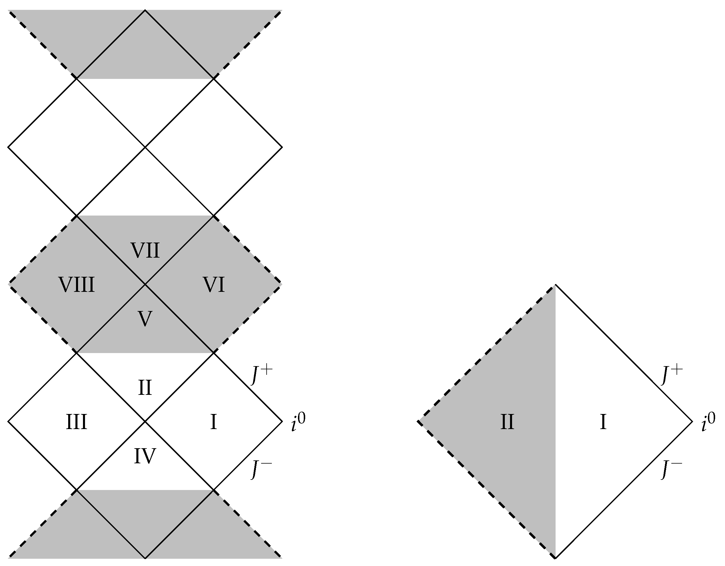
3. Black-Hole Solution

In [13,14], we obtained and described a complete vacuum solution in theory (10) with spherical symmetry. It turns out that the solution respects the Birkhoff theorem: it is necessarily static. This is another manifestation of the absence of new degrees of freedom in the theory. Due to spherical symmetry, the symmetric traceless field ${\mathsf{\Psi }}^{ij}$ has the form

$${\mathsf{\Psi }}^{ij}=\psi \left(r\right)\left(3\frac{x^i{x}^j}{r^2}-{\delta }^{ij}\right),$$

(16)

and is described by a single function $\psi \left(r\right)$ of the radial coordinate $r=\sqrt{{\sum }_i{\left(x^i\right)}^2}$. The cosmological function $\mathsf{\Lambda }\left(\mathsf{\Psi }\right)$ becomes a function of $\psi$, and its derivative with respect to $\psi$, which we denote by ${\mathsf{\Lambda }}_{\psi }$, quantifies the deviation of the theory from GR: The condition $\left|{\mathsf{\Lambda }}_{\psi }\right|$ ≪ 1 implies the validity of GR.

The solution for the gauge field can be found in [13] and is expressed as

$$A^1=f\left(r\right)sin\theta d\varphi ,A^2=-f\left(r\right)d\theta ,A^3=\mathrm{i}\frac{r{r}_g(\infty )}{r_g\left(r\right)}\left[\psi \left(r\right)-\frac{\mathsf{\Lambda }\left(r\right)}{3}\right]dt-cos\theta d\varphi ,$$

(17)

where $\mathsf{\Lambda }\left(r\right)\equiv \mathsf{\Lambda }\left(\psi \left(r\right)\right)$,

$$f\left(r\right)=\sqrt{1-\frac{r_g\left(r\right)}{r}-\frac{1}{3}\mathsf{\Lambda }\left(r\right)r^2},\psi \left(r\right)=\frac{r_g\left(r\right)}{2r^3},$$

(18)

and the function $r_g\left(r\right)$ is determined from the equation

$$r_g\left(r\right)exp\left({\int }_0^{r_g\left(r\right)/2r^3}\frac{{\mathsf{\Lambda }}_{\psi }}{6\psi }d\psi \right)=r_g(\infty ).$$

(19)

The arising metric, specified by the condition of anti-self-duality of the curvature components $F^i$ and by the metric volume form ${\mathcal{V}}_g\propto \mathrm{Tr}B\wedge B$, has the following form:

$$d{s}^2=\left(\frac{1-{\mathsf{\Lambda }}_{\psi }/3}{1+{\mathsf{\Lambda }}_{\psi }/6}\right)\left[\frac{r_g^2(\infty )}{r_g^2\left(r\right)}{f}^2\left(r\right)d{t}^2-f^{-2}\left(r\right)d{r}^2\right]-r^{2}d{\mathsf{\Omega }}^2.$$

(20)

As long as $\left|{\mathsf{\Lambda }}_{\psi }\right|$ ≪ 1, the solution closely follows the Schwarzschild solution. However, in the domain where $\left|{\mathsf{\Lambda }}_{\psi }\right|$ becomes appreciable, it deviates from the Schwarzschild behavior. It turns out to be more appropriate to describe solution in coordinates $(t,\psi )$ rather than $(t,r)$. In this case, the solution can be extended with coordinate r being non-monotonic, and bounded from below. For the theory defined by Equation (11), the corresponding conformal diagram is presented in Figure 1, adopted from [13]. Although the constructed metric (20) becomes singular on the boundaries between grey and white regions in the figure, the fundamental gauge field $A^i$ is regular there. It is in this sense that we can speak about the “resolution” of Schwarzschild black-hole singularity in terms of fundamental connection variables $A^i$. Note that the black-hole horizon in the metric exists only in the case [13]

$$r_g(\infty )>r_c\equiv \frac{2\sqrt{\alpha }}{e{\left(1+\alpha {\mathsf{\Lambda }}_0/3\right)}^{3/2}}.$$

(21)

In the opposite case, one obtains a solution resembling the Schwarzschild case with negative mass.

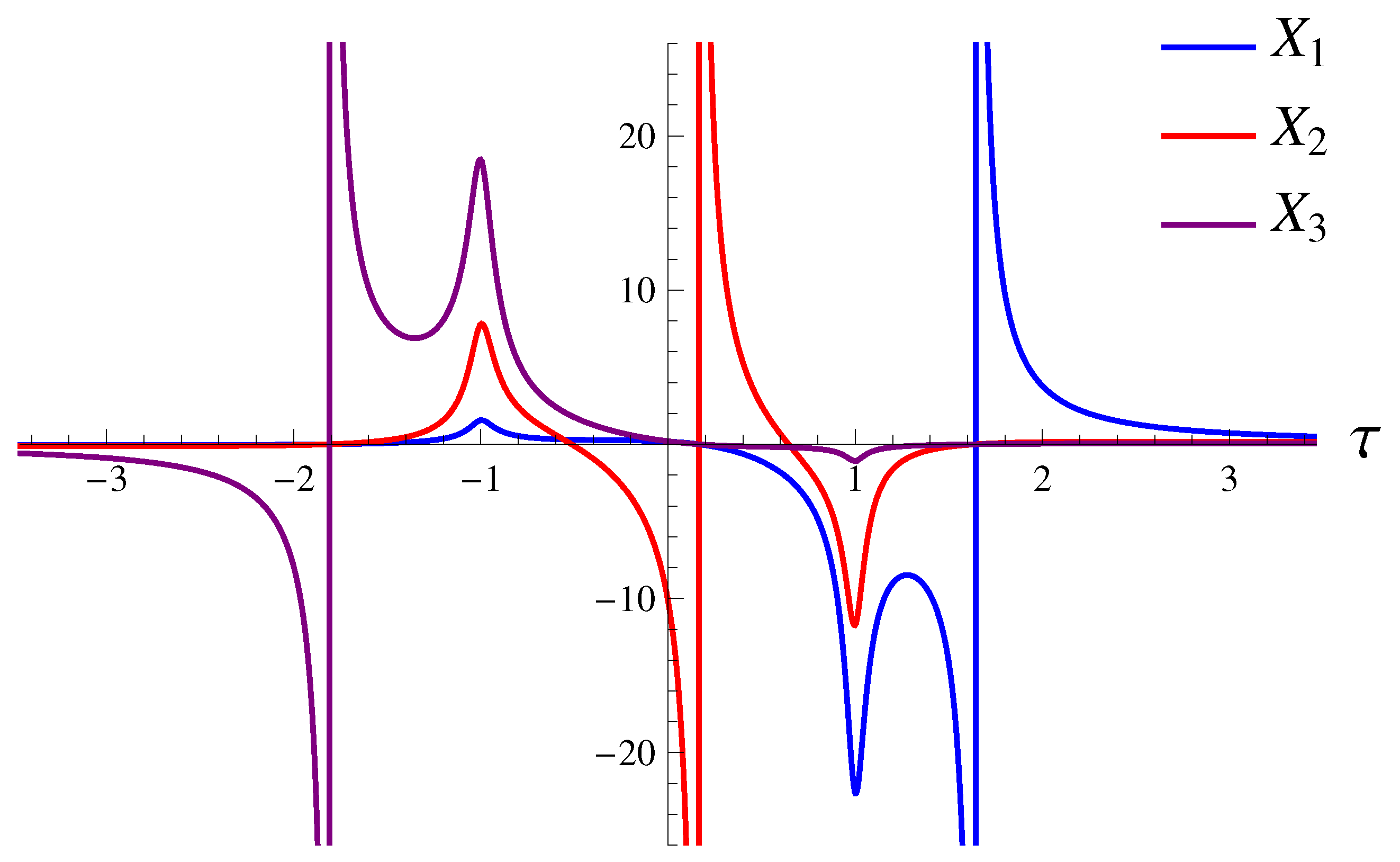
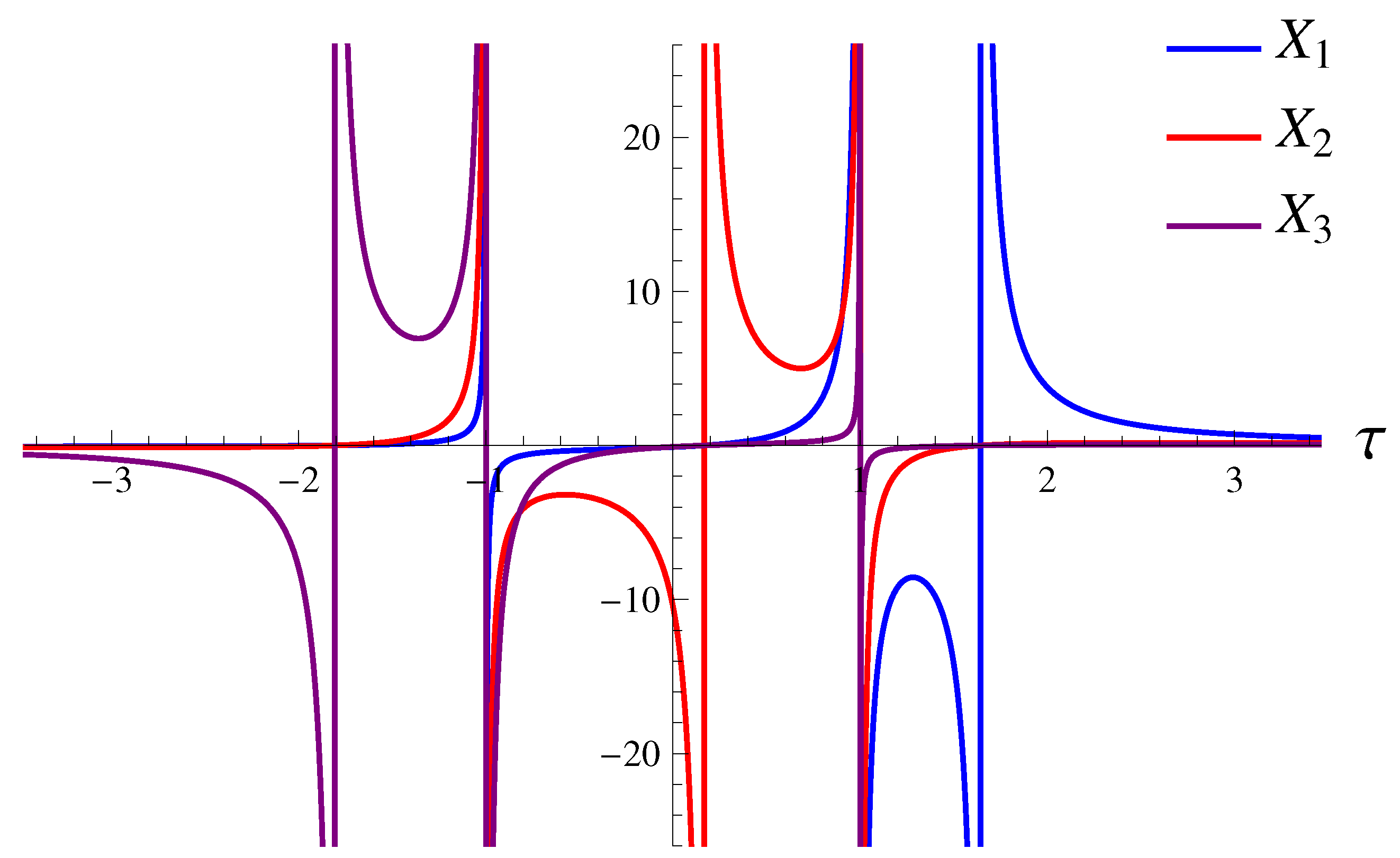
4. Bianchi I Cosmology

In general relativity, Bianchi I cosmological model is described by a spatially Euclidean metric of the form

$$d{s}^2=d{t}^2-{\left[a_1\left(t\right)d{x}^1\right]}^2-{\left[a_2\left(t\right)d{x}^2\right]}^2-{\left[a_3\left(t\right)d{x}^3\right]}^2,$$

(22)

where $a_i\left(t\right)$ are the corresponding scale factors. The so-called Kasner regime is reached as t → 0:

$$a_i^2\sim t^{2p_i},\sum _i{p}_i=1,\sum _i{p}_i^2=1,$$

(23)

and describes approach to singularity at t = 0. In this section, we will show how this singular behavior is “resolved” in the modified theory with the cosmological function (11).

By using the $\mathrm{SO}\left(3\right)$ gauge invariance of the theory, one can write the Bianchi I ansatz for the connection in the form

$$A^k=\mathrm{i}{h}_k\left(\tau \right)d{x}^k(\mathrm{no} \mathrm{sum} \mathrm{over} k),$$

(24)

where $\tau$ is, up to now, an arbitrary time parameter. The corresponding curvature two-form is

$$F^i=d{A}^i+\frac{1}{2}{ϵ}^{ijk}{A}^j\wedge A^k=\mathrm{i}{\dot{h}}_{i}d\tau \wedge d{x}^i-\frac{1}{2}{ϵ}^{ijk}{h}_j{h}_{k}d{x}^j\wedge d{x}^k,$$

(25)

where an overdot denotes derivative with respect to $\tau$. Calculating the wedge product, we obtain

$$F^i\wedge F^j=-2\mathrm{i}{\delta }^{ij}{X}_{i}h{\mathcal{V}}_c,$$

(26)

where ${\mathcal{V}}_c=d\tau \wedge d{x}^1\wedge d{x}^2\wedge d{x}^3$ is the coordinate volume form, $h=h_1{h}_2{h}_3$, and

$$X_i=\frac{{\dot{h}}_i}{h_i}.$$

(27)

If we select the volume form $\mathcal{V}$ in Equation (13) to be

$$\mathcal{V}=-2\mathrm{i}h{\mathcal{V}}_c,$$

(28)

then $X^{ij}$ = $\mathrm{diag}$ $\left(X_1,X_2,X_3\right)$. With this choice of the volume form, the pure-connection formulation Equation (15) reduces to the system

$$\frac{d}{d\tau }\left(\frac{\partial \mathcal{L}}{\partial X_i}\right)=\mathcal{L}\left(X\right)-\frac{\partial \mathcal{L}}{\partial X_i}\sum _j{X}_j,$$

(29)

which is a system of first-order differential equations for $X_i$. By using time-reparametrisation freedom, it is always possible to choose the time variable $\tau$ in such a way that $\mathcal{L}h=\mathrm{const}$. With this choice, and using definition (27), one can integrate Equation (29) to obtain an implicit solution for $X\left(\tau \right)$:

$$\frac{\partial \mathcal{L}\left(X\right)}{\partial X_i}=\mathcal{L}\left(X\right)\left(\tau -{\tau }_i\right),$$

(30)

where ${\tau }_i$ are arbitrary integration constants. Equations (27) and (30) give a complete solution to the problem for an arbitrary theory from our class. Without loss of generality, one can conveniently shift and normalize the time variable so that ${\sum }_i{\tau }_i$ = 0 and ${\sum }_i{\tau }_i^2$ = 6.

The canonical metric of this solution with volume form proportional to $\mathcal{L}\left(X\right)\mathcal{V}$ is given by

$$d{s}^2=\sqrt{\left|\frac{\mathcal{L}\left(X\right){\prod }_i{X}_i}{{\mathsf{\Lambda }}_0}\right|}\left[-d{\tau }^2+\prod _j{X}_j^{-1}\sum _k{h}_k^2{X}_k{\left(d{x}^k\right)}^2\right].$$

(31)

4.1. Behavior in GR

The general solution for $X_i$ in the general relativity theory (14) is given by

$$X_1^{\mathrm{GR}}=\frac{(\tau -{\tau }_2)(\tau -{\tau }_3)}{\sqrt{3}({\tau }^2-1)(\tau -{\tau }_1)},\mathrm{etc}. \mathrm{with} \mathrm{permutation} \mathrm{of} \mathrm{indices}.$$

(32)

The quantities $X_i^{\mathrm{GR}}$ have simple poles at $\tau$ = ${\tau }_i$, and all blow up as $\tau$ → ±1, which corresponds to the Kasner singularity. This behavior is illustrated in Figure 2.

Integrating Equation (27) in the neighborhood of Kasner singularity and using Equation (31), we see that the scale factors behave as

$$a_i^2\sim {(\tau -1)}^{p_i},$$

(33)

where

$$p_1=1-\frac{(1-{\tau }_2)(1-{\tau }_3)}{3({\tau }_1-1)},\mathrm{etc}.$$

(34)

If we arrange the time constants so that ${\tau }_3$ < ${\tau }_2$ < ${\tau }_1$, we obtain the following picture. As $\tau \to \infty$, we approach the De Sitter solution $X_i$ = 1/$\sqrt{3}\tau$. As time decreases, at $\tau$ = ${\tau }_1$ we encounter a special point where $X_1$ has a simple pole, while $X_2$ and $X_3$ vanish. Below this point, all $X_i$ change sign, as does $\mathcal{L}\left(X\right)$. The component of the connection $h_1$ vanishes at this point, while the components $h_2$ and $h_3$ remain finite. All components of the canonical metric (31) remain finite at this point. In terms of metric, this is the point where the Hubble parameter $H_1$ = ${\dot{a}}_1/a_1$ vanishes, and the scale factor $a_1$ reaches its minimum value.

As $\tau \to 1$ in our normalization, we approach the Kasner singularity, with the functions $X_i$ all negative near the singularity, and all having a simple pole there. The scale factors $a_i^2$ exhibit the familiar Kasner behavior (23), with exponents $p_i$ given by Equation (34).

Since the gauge field diverges at the singularity, the domain − 1 < $\tau$ < 1 in Equation (32) can only be treated as another singular solution. The solution in the time interval ${\tau }_2$ < $\tau$ < 1 is described by GR with negative cosmological constant $-{\mathsf{\Lambda }}_0$. The behavior near $\tau$ = 1 is again Kasner. The point ${\tau }_2$ again is a special point of the solution, in which $X_2$ has a simple pole, while $X_1$ and $X_3$ have simple zeros. Thus, $h_2$ passes through zero at this point, with $h_1$ and $h_3$ remaining finite and nonzero. The metric components are all finite and non-zero. As $\tau$ → −1, we encounter another Kasner singularity. Thus, this part of the solution interpolates between two Kasner singularities. There is no asymptotic anti-De Sitter regime in this case.

For $\tau$ < −1, we have another copy of asymptotically De Sitter solution. We note that all $X_i$ are positive near the singularity in this case, as is $\mathcal{L}\left(X\right)$. There is a Kasner singularity as $\tau$ → −1, and a special point at $\tau$ = ${\tau }_3$ with $h_3$ vanishing and all $X_i$ and $\mathcal{L}\left(X\right)$ changing sign. As $\tau \to -\infty$, we approach another De Sitter region. Since the time change $\tau \to -\tau$ makes the region $\tau$ < −1 mathematically equivalent to the asymptotically De Sitter region $\tau$ > 1 discussed above, it is clear that the Kasner exponents near the singularity in the region $\tau$ < −1 are obtained from Equation (34) by the replacement ${\tau }_i$ → −${\tau }_i$.

4.2. Behavior in Modified Gravity

In the modified theory of gravity described by the function $\mathsf{\Lambda }\left(\mathsf{\Psi }\right)$ in Equation (10), it is quite difficult to calculate the corresponding Lagrangian $\mathcal{L}\left(X\right)$ in order to use the general solution (30). In fact, this is difficult to do even in the simple case of modification (11). Therefore, to solve for the gauge-field dynamics, one has to resort to formalism with auxiliary matrix field ${\mathsf{\Psi }}^{ij}$ together with the connection $A^i$—the formalism which is obtained by excluding only the B-field from action (10). This procedure was followed by in our paper [15], where a general solution for the Bianchi I case was obtained in the form

$$X=\frac{T^{-2}\left(\mathrm{Id}-\frac{\partial \mathsf{\Lambda }\left(\mathsf{\Psi }\right)}{\partial \mathsf{\Psi }}\right)}{\mathrm{Tr}\left[T^{-1}\left(\mathrm{Id}-\frac{\partial \mathsf{\Lambda }\left(\mathsf{\Psi }\right)}{\partial \mathsf{\Psi }}\right)\right]},\mathsf{\Psi }=\mathsf{\Lambda }\left(\mathsf{\Psi }\right)\left[\frac{T^{-1}}{\mathrm{Tr}\left(T^{-1}\right)}-\frac{1}{3}\mathrm{Id}\right].$$

(35)

The last equation is to be solved with respect to $\mathsf{\Psi }$, with the result to be substituted into the first equation. Here, $T=\mathrm{diag}\left\{(\tau -{\tau }_i)\right\}$, and $\mathrm{Id}$ is the identity matrix.

For the modified theory (11), we observe that the singular behavior of the variables $X_i$ and connection-field components $h_i$ around $\tau$ = ±1 in GR is replaced by a regular behavior of these quantities. The situation is depicted in Figure 3.

In the general-relativistic solution, all $X_i$ are negative and blow up near the Kasner singularity $\tau$ → 1. Our modification (11) resolves this singularity, making all $X_i$ large negative but finite. Our solution thus smoothly continues to the region $\tau$ < 1. Since $X_i$ are finite and nonzero at this point, $\mathcal{L}\left(X\right)$ is also continuous. However, the value of $\mathsf{\Lambda }\left(\mathsf{\Psi }\right)$ crosses zero and becomes negative at $\tau <1$.

As time decreases from $\tau$ = 1, the next special point that we encounter is $\tau$ = ${\tau }_2$. We observe that $X_1$ and $X_3$ cross zero at $\tau$ = ${\tau }_2$, while $X_2\approx \sqrt{3}/(\tau -{\tau }_2)$ has a simple pole, approaching positive infinity as $\tau \to {\tau }_2$ from above. Since all $X_i$ were negative at $\tau =1$, this means that $X_2$ crosses zero at some ${\tau }_{+}\in ({\tau }_2,1)$. It then crosses zero once again at some ${\tau }_{-}\in (-1,{\tau }_2)$. This behavior is demonstrated in Figure 3. In the interval $({\tau }_{-},{\tau }_{+})$, metric (31) changes signature from $(-,+,+,+)$ to $(-,-,+,-)$, the spatial coordinate $x^2$ thus taking the role of time. Thus, although we do not encounter singularity in the fundamental gauge field (all $h_i$ are everywhere smooth), there is a singularity in metric (31) at the points $\tau$ = ${\tau }_{\pm }$, where it also changes signature.

This behavior is in parallel to the “resolution” of the Schwarzschild singularity discussed in the preceding section, where we also observe change of signature of the corresponding metric. In both cases, it has to do with the fact that the value of $\mathsf{\Lambda }\left(\mathsf{\Psi }\right)$ becomes negative in our model (11) as the quantity $\mathrm{Tr}{\mathsf{\Psi }}^2$ increases. Such a behavior of the “cosmological function” $\mathsf{\Lambda }\left(\mathsf{\Psi }\right)$ saves the theory from singularity.

5. Discussion and Conclusions

In this paper, we considered a specific family of chiral modified gravity theories in four dimensions. In the language of pure connection, the main idea is to consider general homogeneous functions of the curvature of the connection as Lagrangians of the theory. Such a modification is guaranteed to lead to second-order field equations without new degrees of freedom. The fundamental field in this formulation is the connection field; the requirement of its curvature components to be (anti)-self-dual then determines the conformal class of metrics. The metric can thus be regarded as a derived, or secondary concept in this formulation.

The family of modifications under consideration is chiral; therefore, we are dealing with modifications of complexified GR. Such a theory begs for reality conditions, which are not difficult to formulate in the cases of Riemannian and split signatures of the arising metric. In the case of physical Lorentzian signature, no general reality conditions are known. Another closely related problem is coupling of this theory to matter. Note that matter fields in our setting should couple to the fundamental field describing gravity, which is the connection field. Alternatively, one can start with a more general family of gauge theories [16] that describe gravity as well as matter fields. The problem of reality conditions will remain in any setting; since matter fields couple to a complex-valued connection, some reality conditions are required to make sense of the arising dynamics.

In some special cases, such as the spherically symmetric case or the Bianchi I setup, the problem of reality causes no difficulty: the self-dual part of the Weyl curvature is automatically real, resulting in real effective metrics. Our main finding in these cases is that a natural one-parameter family of modifications (11) with positive parameter $\alpha$ resolves the Schwarzschild black-hole and Kasner singularities. In the spherically symmetric case, we obtain a space-time extending indefinitely and periodically beyond the would-be black-hole singularity (see Figure 1). In the case of Bianchi I symmetry, we obtain a solution bypassing the would-be Kasner singularities and connecting two asymptotically De Sitter regions (see Figure 3). In both space-times, the fundamental connection field remains regular, although the related metric has singularity points with changes of signature along some coordinates. This type of metric singularity, in the absence of singularity in the basic connection field, appears to be generic to the family of modified theories under investigation. The fact that chiral modified gravity theories can resolve the singularities of general-relativistic solutions is quite remarkable and makes them worth further investigation.

References

1. Starobinsky, A.A. A New Type of Isotropic Cosmological Models Without Singularity. Phys. Lett. B 1980, 91, 99–102. [Google Scholar] [CrossRef]
2. Ade, P.A.R.; Aghanim, N.; Arnaud, M.; Arroja, F.; Ashdown, M.; Aumont, J.; Baccigalupi, C.; Ballardini, M.; Banday, A.J.; Barreiro, R.B.; et al. Planck 2015 results. XX. Constraints on inflation. Astron. Astrophys. 2016, 594, A20. [Google Scholar] [CrossRef]
3. Plebański, J.F. On the separation of Einsteinian substructures. J. Math. Phys. 1977, 18, 2511–2520. [Google Scholar] [CrossRef]
4. Bengtsson, I. The Cosmological constants. Phys. Lett. B 1991, 254, 55–60. [Google Scholar] [CrossRef]
5. Krasnov, K. Renormalizable non-metric quantum gravity? arXiv, 2006; arXiv:hep-th/0611182. [Google Scholar]
6. Eddington, A.S. The Mathematical Theory of Relativity; Cambridge University Press: Cambridge, UK, 1920; Chapter 7. [Google Scholar]
7. Schrödinger, E. Space-Time Structure; Cambridge University Press: Cambridge, UK, 1950; Chapter 12. [Google Scholar]
8. Capovilla, R.; Jacobson, T.; Dell, J.; Mason, L. Self-dual 2-forms and gravity. Class. Quantum Gravity 1991, 8, 41–57. [Google Scholar] [CrossRef]
9. Krasnov, K. Plebański formulation of general relativity: A practical introduction. Gen. Relativ. Gravit. 2011, 43, 1–15. [Google Scholar] [CrossRef]
10. Urbantke, H. On integrability properties of Su(2) Yang–Mills fields. I. Infinitesimal part. J. Math. Phys. 1984, 25, 2321–2324. [Google Scholar] [CrossRef]
11. Krasnov, K. On deformations of Ashtekar’s constraint algebra. Phys. Rev. Lett. 2008, 100, 081102. [Google Scholar] [CrossRef] [PubMed]
12. Krasnov, K. Pure connection action principle for general relativity. Phys. Rev. Lett. 2011, 106, 251103. [Google Scholar] [CrossRef] [PubMed]
13. Krasnov, K.; Shtanov, Y. Non-metric gravity: II. Spherically symmetric solution, missing mass and redshifts of quasars. Class. Quantum Gravity 2008, 25, 025002. [Google Scholar] [CrossRef]
14. Krasnov, K.; Shtanov, Y. Halos of modified gravity. Int. J. Mod. Phys. D 2009, 17, 2555–2562. [Google Scholar] [CrossRef]
15. Herfray, Y.; Krasnov, K.; Shtanov, Y. Anisotropic singularities in chiral modified gravity. Class. Quantum Gravity 2016, 33, 235001. [Google Scholar] [CrossRef]
16. Krasnov, K. Spontaneous symmetry breaking and gravity. Phys. Rev. D 2012, 85, 125023. [Google Scholar] [CrossRef]
Figure 1. Conformal diagram of the spherically symmetric solution with the Lambda-function (11) and with the Schwarzschild radius r g ( ) > r c (left image) and r g ( ) < r c (right image), with r c given in Equation (21). Different regions are numbered in such a way that the coordinate t is timelike in the odd regions, and spacelike in the even ones. The flow of time is vertical in the white regions and changes to horizontal in the grey regions. The boundaries between grey and white regions are places where metric changes signature and, therefore, becomes singular. Thick dashed lines indicate the true singularity, where r = ∞ and ψ = ∞. The configuration on the left image extends periodically and indefinitely upward and downward. We are living in one of the regions of type I; the asymptotic spatial infinity in this region is denoted by i 0 , and the future and past null infinities are denoted by J + and J , respectively.
Universe 04 00012 g001
Figure 2. Behavior of the variables X i given by Equation (30) in general relativity. Each variable X i has a pole at respective τ = τ i . These are just special points of the solution, with all connection and metric components remaining finite. Furthermore, all variables X i have common poles at τ = ±1. These are the singular points for both the connection and the metric. The region “between” two Kasner singularities describes a solution with negative Λ , while the two outer regions describe solutions with Λ > 0.
Universe 04 00012 g002
Figure 3. Behavior of the variables X i given by Equation (35) in the modified theory (11) with α Λ 0 = 5 × 10 3 . As in general relativity (see Figure 2), each variable X i has a pole at respective τ = τ i . However, the common poles at τ = ±1 disappear, and the variables X i become regular at these points.
Universe 04 00012 g003