Semi-Classical Particle Production in Bouncing Cosmologies

Abstract

We study semi-classical particle production in non-singular bouncing cosmologies by employing the Unruh–DeWitt model of a particle detector. Rather than approximating the scale factor in different regimes of energy domination, the scale factor for the bouncing cosmology is obtained numerically by solving a modified Friedmann–Lemaître equation obtained from the semi-classical limit of a loop quantum cosmology model. We examine how the detector response varies with the energy density at the bounce and the energy gap of the detector, and we also compare our exact numerical results with analytical approximations in the literature.

1. Introduction

In 1931, Georges Lemaître’s seminal article in Nature [1] proposed that the entire cosmos began with a single “primeval atom”, an idea later termed the big bang model by steady-state proponent Sir Fred Hoyle. While the Big Bang model fit with Hubble’s discovery that the galaxies were receding away from one another at a rate proportional to their distance [2], it was not until the 1970s that the Big Bang model gained wide acceptance among cosmologists. The acceptance was precipitated by the discovery of the cosmic microwave radiation by Penzias and Wilson [3]. The Big Bang turned out to explain a broad plethora of cosmological phenomena, from the abundance of the light elements to structure formation, and today is the widely accepted cosmological paradigm.

Notwithstanding its explanatory success, Big Bang cosmologies present some obvious problems that were already apparent to Lemaître at the inception of the theory. He writes [1] “If the world has begun with a single quantum, the notions of time and space would altogether fail to have any meaning at the beginning …”. He is, of course, referring to the Big Bang singularity, a point in the past where the energy density and curvature of the universe are infinite, i.e., the very notion of spacetime itself has broken down. Moreover, the classical Big Bang model brings with it other issues apart from the singularity, including the horizon, inhomogeneity, and flatness problems [4]. Despite the success and popularity of inflation as a means of resolving some of these issues, there remain open questions about the fine-tuning of parameters and specific initial conditions [5,6] for the inflaton field, as well as questions about its observability.

An alternative solution to both the singularity problem and the various fine-tuning issues is to assume a model of cosmological evolution that replaces the Big Bang with a Big Bounce [7]. These are the models that we study in this paper. From the Hawking-Penrose singularity theorems [8], we know that, classically, the Big Bang singularity is unavoidable unless we violate at least one of the energy conditions or unless we modify the Einstein equations. With these options, many non-singular models have been proposed, including the matter bounce scenario involving potentially exotic matter discussed by Brandenburger et al. in Refs. [9,10], energy condition violating models like those proposed by Steinhardt and Ijjas in Refs. [4,11], or by considering models that arise in modified gravity through higher-derivative corrections to the gravitational action, see, for example, Ref. [12].

In scenarios where the characteristic length scale associated with the bounce becomes sufficiently small–specifically approaching the Planck length–then the quantum nature of spacetime can no longer be neglected. One approach to combining general relativity and quantum mechanics that has been shown to produce a cosmological bounce is loop quantum gravity (LQG) [13]. Utilizing a well-defined semi-classical limit to LQG, Ref. [14] derives a modified Friedmann–Lemaître equation containing leading-order quantum corrections. The quantum correction becomes non-negligible at very high energy densities and acts as an effective repulsive gravitational force, producing a bounce rather than a singularity, while the semi-classical correction to the Friedmann–Lemaître equation is formally valid only at times late enough that the quantum nature of spacetime itself can be ignored. It is argued in Ref. [15] that the semi-classical limit of LQG still produces surprisingly accurate predictions at earlier times. In particular, both the full loop quantum cosmology simulations and the semi-classical limit both produce bouncing models, which is the main feature we are interested in. In any case, our philosophy here is more phenomenological than fundamental, and we simply take as the governing equations of the universe a modified Friemann–Lemaître equation quite independent from its hierarchical theory. Additionally, we do not consider scenarios in which the scale of the universe is close to the Planck length, i.e., the spacetimes we examine are considered classical at all times. In fact, it is crucial for the internal consistency of our framework that we remain outside a regime where quantum gravitational effects become significant. This assumption underlies our adoption of the Unruh–DeWitt particle detector model, which operates within the framework of quantum field theory in curved spacetimes. Thus, we simply take this effective Friedmann–Lemaître equation as our governing equation for the dynamics of the universe.

In this paper, we use this Modified Friedmann–Lemaître equation (MFLE) to numerically generate non-singular, bouncing cosmologies and then utilize the Unruh–DeWitt particle detector to examine the bounce’s effects on cosmological particle production. We also observe how the detector’s response adapts to variations in the magnitude of the leading-order quantum correction in the MFLE or the gap between energy eigenvalues of the detector model. Finally, we compare the response of the detector between our MFLE models and a classical Big Bang cosmology. Knowing that the detector is highly localized in spacetime, one might assume it would be insensitive to whether the universe began with a bang or a bounce, or indeed whether a bounce was gradual or sharp. However, as will be seen, the detector’s response at any time is shaped by its full history. Moreover, the quantum scalar field that couples to the detector must be prepared in a quantum state. Both of these facts mean that the detector probes global features of the spacetime and can ostensibly have an imprint of the bounce even at late times, albeit a very small one.

A secondary focus of this paper is to compare our findings with those from recent similar work in Ref. [16]. Their approach to modeling bouncing cosmologies required analytically solving the MFLE in the contraction, bounce, matter-domination, and $\Lambda$-domination epochs, only taking into account the corresponding dominant energy density term in each era, and then gluing the exact solutions together. One issue with that approach is that there is enough freedom in the model to match the scale factors and their derivatives, but not their second derivatives. The points of transition between the different epochs can produce unphysical noise in the detector response. This issue is circumvented in this paper by solving the full equations numerically, making no approximations in the various regimes. The result is a scale factor that is smooth to all orders throughout its history, producing no undesirable transient effects in the detector response as the various epochs are traversed by the detector.

This paper is organized as follows: We begin Section 2 with an introduction to classical bouncing cosmologies, which we use to motivate our adoption of the MFLE. After formulating the MFLE and observing some of the associated phenomenology, Section 3 derives the transition rate for an Unruh–DeWitt particle detector coupled to a quantum scalar field in this spacetime and describes our methods for calculating its response. In Section 4, we present results for the response rates for the Unruh–DeWitt particle detector for a range of parameters. Finally, our review and conclusions are given in Section 5.

2. The Modified Friedmann–Lemaître Equation

2.1. Friedmann–Lemaître Equation

Assuming the cosmological principle that the spatial slices of the universe are homogeneous and isotropic, the spacetime metric in spherical polar coordinates is given by the Robertson-Walker form [17]

$$\begin{array}{c}\hfill d{s}^2=-d{t}^2+a^2\left(t\right)\left({\displaystyle \frac{d{r}^2}{1-k{r}^2}}+r^{2}d{\theta }^2+r^2{sin}^2\theta d{\varphi }^2\right),\end{array}$$

(1)

where $a\left(t\right)$ is the scale factor of the universe and k is an arbitrary constant. The intrinsic Gaussian curvature of the constant t hypersurfaces is

$$\begin{array}{c}\hfill K\left(t\right)={\displaystyle \frac{k}{a^2\left(t\right)}}.\end{array}$$

(2)

Positive k then implies positive $K\left(t\right)$, and these universes are defined to be closed. This classification is logically independent of whether the universe recollapses. A universe that is not closed is open, which corresponds to $k\le 0$.

The statements above are purely kinematical. For the dynamics, we require evolution equations for the scale factor $a\left(t\right)$. Assuming the stress-energy tensor for non-interacting perfect fluids of baryonic matter and radiation, Einstein’s equations combined with stress-energy conservation yield the well-known Friedmann–Lemaître equation

$$\begin{array}{c}\hfill {\displaystyle \frac{{\dot{a}}^2\left(t\right)}{a^2\left(t\right)}}={\displaystyle \frac{8\pi G}{3}}{\displaystyle \frac{{\rho }_{m,0}}{a^3\left(t\right)}}+{\displaystyle \frac{8\pi G}{3}}{\displaystyle \frac{{\rho }_{r,0}}{a^4\left(t\right)}}-{\displaystyle \frac{k}{a^2\left(t\right)}}+{\displaystyle \frac{\Lambda }{3}},\end{array}$$

(3)

where ${\rho }_{m,0}$ and ${\rho }_{r,0}$ are, respectively, the matter and radiation energy density at the present epoch, which we assume corresponds to $t=0$. Given values for the constants $\{{\rho }_{m,0},{\rho }_{r,0},k,\Lambda \}$ along with the boundary conditions for the scale factor, one could employ the Friedmann–Lemaître equations to predict or retrodict the entire evolution of the universe. It is convenient to express the energy densities in terms of dimensionless parameters. Normalizing the scale factor so that $a\left(0\right)=1$, then the Hubble parameter today is $H_0=\dot{a}\left(0\right)$ so that Equation (3) evaluated today gives

$$\begin{array}{c}\hfill 1={\Omega }_m+{\Omega }_r+{\Omega }_k+{\Omega }_{\Lambda }\end{array}$$

(4)

where

$$\begin{array}{c}\hfill {\Omega }_m={\displaystyle \frac{{\rho }_{m,0}}{{\rho }_{\mathrm{tot},0}}},{\Omega }_r={\displaystyle \frac{{\rho }_{r,0}}{{\rho }_{\mathrm{tot},0}}},{\Omega }_k=-{\displaystyle \frac{3k}{8\pi G{\rho }_{\mathrm{tot},0}}},{\Omega }_{\Lambda }={\displaystyle \frac{\Lambda }{8\pi G{\rho }_{\mathrm{tot},0}}}\end{array}$$

(5)

with ${\rho }_{\mathrm{tot},0}=3H_0^2/\left(8\pi G\right)$. We interpret these parameters in Equation (5) as the dimensionless contributions to the total energy density today coming from matter, radiation, curvature, and the cosmological constant, respectively, and keep in mind that the latter two contributions can be negative. Finally, we will also find it convenient to rescale the time to dimensionless cosmic time $\lambda =H_{0}t$, whence the Friedmann–Lemaître equation takes the form

$$\begin{array}{c}\hfill {\mathcal{H}}^2\left(\lambda \right)={\displaystyle \frac{{\Omega }_m}{a^3\left(\lambda \right)}}+{\displaystyle \frac{{\Omega }_r}{a^4\left(\lambda \right)}}+{\displaystyle \frac{(1-{\Omega }_m-{\Omega }_r-{\Omega }_{\Lambda })}{a^2\left(\lambda \right)}}+{\Omega }_{\Lambda }\end{array}$$

(6)

where $\mathcal{H}\left(\lambda \right)=a^{\prime }\left(\lambda \right)/a\left(\lambda \right)$ and throughout $\prime$ represents a derivative with respect to $\lambda$. We have also used (4) to eliminate any explicit dependence on the Gaussian curvature.

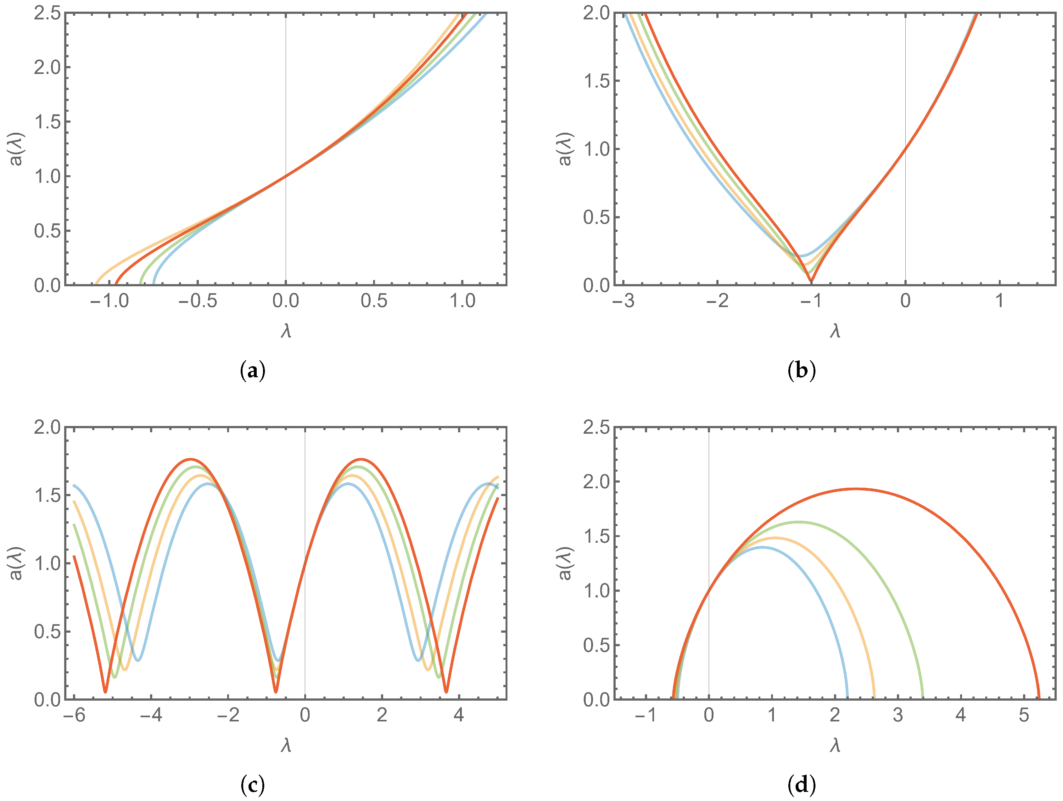
If we assume values of the density parameters in concordance with the standard $\Lambda$CDM model, ${\Omega }_m=0.3$, ${\Omega }_r=8.4\ast {10}^{-5}$, and ${\Omega }_{\Lambda }=0.7$ [18] (what we refer to as benchmark values), then one finds that $a\to 0$ at $\lambda \approx -1$, corresponding to the Big Bang singularity at approximately $t=-H_0^{-1}$. It is worth pointing out, however, that the phenomenology of solutions to Equation (6) is very diverse. In Figure 1, we illustrate a selection of these model types: Big Bang models leading to eternal expansion, non-singular big bounce and cyclic models, and big crunch models displaying re-collapse to a singularity. However, to produce cosmologies very different from the standard Big Bang scenario, we necessarily pick parameter values that have some disagreeable features. For example, the models containing non-singular bounces, like those in Figure 1b,c, usually require a negative energy density for radiation, clearly violating the null energy condition. It is precisely this violation that acts as an effective repulsive gravitational force when radiation is the dominant energy form, and thus leads to a bounce.

Now, given the explanatory success of the Big Bang model, we would like to explore the possibility of bouncing models while being as conservative as possible. In other words, we would like to ameliorate the conceptual and philosophical issues associated with spacetime possessing a spacetime singularity while preserving our standard model for times later than the radiation domination epoch. As we have seen, we can obtain bouncing models from the Friedmann–Lemaître equations without any modification, but these bouncing scenarios require density parameters that do not appear to coincide with observed data. So the guiding principles for our bouncing cosmology are (i) the model should employ density parameters that agree with $\Lambda$CDM benchmark values, (ii) the model should correspond to the standard solution of the classical Friedmann–Lemaître equation at late times after the bounce, and (iii) the bounce should occur approximately at the time of the Big Bang in the corresponding Friedmann-Lamaître model. To obtain such a solution, we turn to a modification of the Friedmann-Lamaître equations above, which we describe in the next section.

2.2. Modified Friedmann–Lemaître Equation

To obtain our bouncing model, we begin with the same assumption of a homogeneous, isotropic universe with the Robertson-Walker metric (1). The distinction is that rather than assume Einstein’s equations, which lead to the Friedmann–Lemaître equations, we assume that the scale factor satisfies the following modified equation

$$\begin{array}{c}\hfill H^2\left(t\right)={\displaystyle \frac{{\dot{a}}^2\left(t\right)}{a^2\left(t\right)}}={\displaystyle \frac{8\pi G}{3}}\rho \left(t\right)\left(1-{\displaystyle \frac{\rho \left(t\right)}{{\rho }_b}}\right),\end{array}$$

(7)

where ${\rho }_b$ is a constant density parameter that determines the magnitude of the correction to the standard Friedmann–Lemaître model. This approach is inspired by a semi-classical limit of a Loop Quantum Cosmology formulation (see, for example, Ref. [14]). Despite its derivation via LQC, we choose to take a phenomenological approach to our model, assuming Equation (7) as our evolution equation untethered to any particular gravitational or quantum gravitational theory.

Following essentially the same process as in Section 2.1, we incorporate the non-interacting fluids of matter and radiation, along with the cosmological constant and Gaussian curvature. For simplicity and to ensure we generate similar models to those found in Ref. [16], we choose to only include the quantum-correction bounce-inducing term within the energy density of radiation, as it is the dominant energy near the classical singularity or our bounce region, i.e., whenever $a\left(t\right)<<1$. With the same condition that $t=0$ corresponds to the present time and that $a\left(0\right)=1$, we obtain the following form of the modified Friedmann–Lemaître equation (MFLE),

$$\begin{array}{c}\hfill {\mathcal{H}}^2\left(\lambda \right)={\displaystyle \frac{{\Omega }_m}{a^3\left(\lambda \right)}}+{\displaystyle \frac{{\Omega }_r}{a^4\left(\lambda \right)}}\left(1-{\displaystyle \frac{1}{a^4\left(\lambda \right)}}{\displaystyle \frac{{\Omega }_r}{{\Omega }_b}}\right)+{\Omega }_{\Lambda }+{\displaystyle \frac{{\Omega }_k}{a^2\left(\lambda \right)}},\end{array}$$

(8)

where ${\Omega }_b={\rho }_b/{\rho }_{\mathrm{tot},0}$. Evaluating the above equation at the present time yields ${\Omega }_k=1-({\Omega }_m+{\Omega }_r-{\Omega }_r^2/{\Omega }_b+{\Omega }_{\Lambda })$, which can be used to eliminate the dependence on the energy density of the intrinsic curvature.

In this form, the parameter $\alpha ={\Omega }_r/{\Omega }_b$ represents the relative scale at which the semi-classical effects introduced in the MFLE become dominant. Clearly at small scale factors, the terms involving ${\Omega }_r$ dominate, and so we have that in this regime ${\mathcal{H}}^2\left(\lambda \right)\approx 0$ whenever $a^4\left(\lambda \right)\approx \alpha$. A larger value for $\alpha$ implies a more recent bounce at higher values of the scale factor compared with smaller values of $\alpha$. Conversely, a small value for $\alpha$ implies a bounce will occur when the scale factor is very small, and we would expect these models to have observational signatures close to those of standard Big Bang cosmologies derived from Einstein’s equations. Setting $\alpha =0$, or equivalently ${\Omega }_b\to \infty$, retrieves precisely the classical Friedmann–Lemaître equation. The most conservative model that is free from spacetime singularities and yet has observational signatures very similar to our standard model is one with small $\alpha$ (or large ${\Omega }_b$) and which assumes other density parameters equal to their benchmark values $({\Omega }_m=0.3$, ${\Omega }_r=8.4·{10}^{-5}$, ${\Omega }_{\Lambda }=0.7)$. We will also sometimes permit $\alpha$ to be non-negligible in order to clearly distill the effect of this parameter on the rate of particle production.

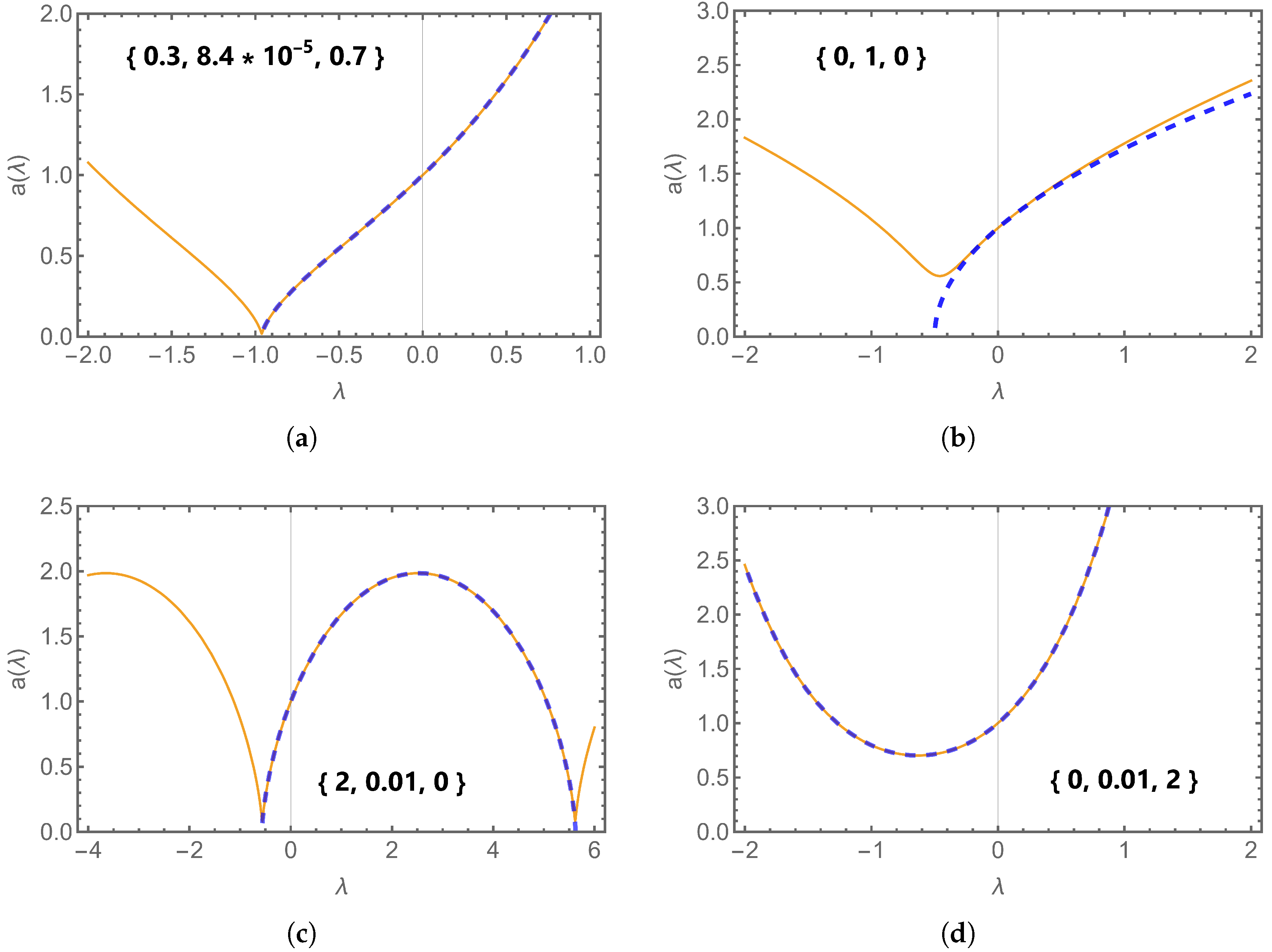
To illustrate the general effect the bounce-inducing term in the MFLE has on cosmological evolution, we plot eight different models in Figure 2. Each sub-figure contains two models: a blue, dashed curve obeying the classical Friedmann–Lemaître equation and a solid, orange curve obeying the MFLE. It is clear from these plots that the evolution is virtually unchanged in regions where radiation is not the dominant form of energy. As each model evolves backward in time from the present epoch, if the parameter choices permit the scale factor to become very small, then the bounce term in the MFLE dominates and acts like a repulsive gravitational force, whereas the classical models tend to a singularity ($a\to 0$). For some parameter choices, the classical model is non-singular, and the scale factor never reaches a point where radiation becomes the dominant energy form. In these cases, there is no difference between the classical and MFLE models. An example of this type is shown in Figure 2d.

Now we will be solving Equation (8) numerically without recourse to analytical approximations. To do this, we use the in-built ODE solver in Mathematica. To solve the equation numerically, it is preferable to differentiate Equation (8) again and work with the second-order equation. This avoids complications associated with taking the correct branch of the square root in (8). One would have to take the positive root whenever the universe is expanding and the negative root whenever it is contracting and paste the two solutions at the bounce point. However, if we work directly with the second-order equation, then we can integrate the equation across the bounce points without this consideration. Differentiating (8) with respect to $\lambda$ gives

$$\begin{array}{c}\hfill a^{″}\left(\lambda \right)={\displaystyle \frac{1}{2}}\left(-{\displaystyle \frac{{\Omega }_m}{a^2\left(\lambda \right)}}-{\displaystyle \frac{2{\Omega }_r}{a^3\left(\lambda \right)}}+{\displaystyle \frac{6{\Omega }_r^2}{{\Omega }_b{a}^7\left(\lambda \right)}}+2{\Omega }_{\Lambda }a\left(\lambda \right)\right).\end{array}$$

(9)

For our initial conditions, we normalize the scale factor to be unity at the present epoch, $a\left(0\right)=1$, and since $\dot{a}\left(t\right)=H_0{a}^{\prime }\left(\lambda \right)$, we must also have $a^{\prime }\left(0\right)=1$. Finally, evaluating (9) at $\lambda =0$, we obtain $a^{″}\left(0\right)=\frac{1}{2}(-{\Omega }_m-2{\Omega }_r+6{\Omega }_r^2/{\Omega }_b+2{\Omega }_{\Lambda })$. Going forward, our solutions to the MFLE will be numerically generated from Equation (9) with the aforementioned initialization values and calculated to an accuracy of twenty-five decimal places.

As mentioned above, a secondary focus of this work is to compare our results with those from Ref. [16], in which the response of a particle detector is studied when the geometry is determined by analytical approximations to Equation (8). In this approach, whereby approximate solutions are considered, the authors solve analytically Equation (8) in the contraction, bounce, matter-domination, and $\Lambda$-domination epochs, only taking into account the corresponding dominant energy density term. These solutions are then glued together to form a piecewise representation of the scale factor over the history of the universe. There is enough freedom in the integration constants to ensure the continuity of the scale factor and its first derivative across the transitions between the epochs. However, there is not enough freedom in the analytical model to ensure the smoothness of the first derivative. The fact that the derivative is continuous but not smooth in the transitions between epochs can produce nonphysical artifacts in the detector response as it traverses these transition points. These nonphysical artifacts can be quite pronounced near the transitions, obscuring the actual physics of the problem. Thus, a major benefit of numerically solving the MFLE is that the solution is infinitely smooth over the entire domain, and so the detector response does not produce these unwanted artifacts. As well as this, including only the dominant energy density is too crude an approximation in some regimes, especially those regimes close to a transition between epochs, while there is a computational cost associated with our spacetime metric being determined numerically rather than analytically, the cost is not prohibitively high and is more faithful to the physics of the problem.

3. The Unruh–DeWitt Particle Detector

3.1. Formulation

Armed with our MFLE, we now seek to examine semi-classical particle production in these bouncing universes. In particular, we consider the response of an Unruh–DeWitt particle detector [19] as it propagates through the bounce epoch of our non-singular cosmological models.

The Unruh–DeWitt particle detector focuses on the interaction between a two-level idealized atom and a massless quantum scalar field. The system is initialized such that the quantum field, $\widehat{\varphi }\left(x\right)$, is in the state $|{\Phi }_i\rangle$ on some background, and the atom, or detector, is in an initial eigenstate $|E_i\rangle$. The detector registering a particle corresponds to an excitation by absorption of a field quanta, where the atom transitions to the excited state $|E_f\rangle$ and the field to $|{\Phi }_f\rangle$. Alternatively, the detector can de-excite by emitting a field quanta, where the atom transitions from $|E_f\rangle$ to $|E_i\rangle$ and the field from $|{\Phi }_f\rangle$ to $|{\Phi }_i\rangle$. A key aspect of this detector model is that the probability of these transitions occurring is dependent upon the difference between energy eigenvalues, $E=E_f-E_i$, and not on the value of the eigenvalues themselves. We refer to this difference as the energy gap. Treating the interaction between the detector and the field as weak and assuming the interaction is mediated by a switching function of compact support so that the interaction is switched on only for a finite time, one can employ perturbation theory to compute the probability of finding the detector in the excited state $|E_f\rangle$ after the interaction is turned off. Up to an overall constant of proportionality, the transition probability is

$$\begin{array}{c}\hfill \mathcal{F}\left(E\right)=-{\displaystyle \frac{E}{4\pi }}{\int }_{-\infty }^{\infty }{\chi }^2\left(u\right)du+{\displaystyle \frac{1}{2{\pi }^2}}{\int }_0^{\infty }{\displaystyle \frac{ds}{s^2}}{\int }_{-\infty }^{\infty }\chi \left(u\right)\left[\chi \left(u\right)-\chi (u-s)\right]du\\ \hfill +2{\int }_{-\infty }^{\infty }du\chi \left(u\right){\int }_0^{\infty }\chi (u-s)\left[cos\left(Es\right)W(u,u-s)+{\displaystyle \frac{1}{4{\pi }^2{s}^2}}\right]du,\end{array}$$

(10)

where $\chi \left(u\right)$ is the switching function that determines how the interaction between the field and the detector is switched on and off. The bi-distribution $W(u,u-s)\equiv \langle {\Phi }_i\left|\widehat{\varphi }\left(x\left(u\right)\right)\widehat{\varphi }\left(x(u-s)\right)\right|{\Phi }_i\rangle$ is the Wightman two-point function for the quantum scalar in its initial quantum state, evaluated along the worldline of the detector at proper times u and $u-s$. The counterterm in the integrand, $1/\left(4{\pi }^2{s}^2\right)$, explicitly regularizes the Wightman two-point function, ensuring that the distribution is well-defined at the vertex of the detector’s light cone (when $s=0$), provided that the scalar field is in a quantum state that satisfies the Hadamard condition (see, for example, Ref. [20]).

Ideally we would like to switch the detector on and off instantaneously so that the transition probability does not depend strongly on the profile of the switching function. This would mean choosing a sharp switching function of the form

$$\begin{array}{c}\hfill \chi \left(u\right)=\Theta (u-{\tau }_{\mathrm{on}})\Theta (\tau -u),\end{array}$$

(11)

where $\Theta \left(z\right)$ is the Heaviside step function, ${\tau }_{\mathrm{on}}$ is the time the interaction is switched on, and $\tau$ is the detector’s proper time. The problem is that in this sharp switching limit, the transition probability diverges and hence has no meaning. Nevertheless, the instantaneous transition rate, denoted by ${\dot{\mathcal{F}}}_{\tau }\left(E\right)$, is well defined in the sharp switching limit. This corresponds to the derivative of the transition probability with respect to proper time $\tau$. The explicit expression for the transition rate is [20,21]

$$\begin{array}{c}\hfill {\dot{\mathcal{F}}}_{\tau }\left(E\right)=2{\int }_0^{\Delta \tau }\left(cos\left(Es\right)W(\tau ,\tau -s)+{\displaystyle \frac{1}{4{\pi }^2{s}^2}}\right)ds-{\displaystyle \frac{E}{4\pi }}+{\displaystyle \frac{1}{2{\pi }^2\Delta \tau }}\end{array}$$

(12)

where $\Delta \tau =\tau -{\tau }_{\mathrm{on}}$ is the total detection time. This quantity will be our primary interest for the remainder of this article. Physically, up to an overall constant of proportionality, the quantity in (12) corresponds to the number of excitations per unit proper time in an ensemble of identical detectors. If one was to compute this quantity for a uniformly accelerated detector for a quantum field in Minkowski spacetime, it would yield a Planckian thermal spectrum independent of $\tau$. This is the Unruh effect [19].

Looking now at our specific cosmological background, the FLRW metric (1) is conformal to Minkowski spacetime, meaning it can be written as $d{s}^2=a^2\left(\eta \right)[-d{\eta }^2+d{\mathbf{x}}^2]$, where $\eta$ is conformal time defined by

$$\begin{array}{c}\hfill \eta \left(\tau \right)={\int }^{\tau }{\displaystyle \frac{1}{a\left({\tau }^{\prime }\right)}}d{\tau }^{\prime }.\end{array}$$

(13)

For a conformally coupled quantum scalar field (one that satisfies $(\square -\frac{1}{6}R)\varphi =0$) in the conformal vacuum, the Wightman two-point function is conformal to the corresponding two-point function in Minkowski spacetime [21] and is given by

$$\begin{array}{c}\hfill W(x,x^{\prime })={\displaystyle \frac{1}{4{\pi }^{2}a\left(\eta \right)a\left({\eta }^{\prime }\right)}}{\displaystyle \frac{1}{(-\Delta {\eta }^2+\Delta {\mathbf{x}}^2)}}\end{array}$$

(14)

where $\Delta \eta =\eta -{\eta }^{\prime }$ and $\Delta \mathbf{x}=\mathbf{x}-{\mathbf{x}}^{\prime }$. For simplicity, we take the case of a detector comoving with the Hubble flow: $\tau =\lambda /H_0$ and $x=$ constant, where we have again introduced the dimensionless cosmic time $\lambda$. We also prefer to formulate our expression for the transition rate completely in terms of dimensionless quantities. This requires us to define the dimensionless energy gap $\tilde{E}=E/H_0$ and scale the integration variable by $\tilde{s}=H_{0}s$. Then the conformal time along the detector’s trajectory $\eta =\eta \left(\tau \right)$ and $\Delta \eta =\eta -{\eta }^{\prime }=\eta \left(\tau \right)-\eta (\tau -s)$ can be written as

$$\begin{array}{c}\hfill \eta \left(\lambda \right)={\int }^{\lambda }{\displaystyle \frac{d{\lambda }^{\prime }}{a\left({\lambda }^{\prime }\right)}},\Delta \eta ={\int }_{\lambda -\tilde{s}}^{\lambda }{\displaystyle \frac{d{\lambda }^{\prime }}{a\left({\lambda }^{\prime }\right)}}.\end{array}$$

(15)

Finally, in terms of these dimensionless parameters, we write the transition rate for a comoving detector coupled to a conformally invariant quantum scalar field as

$$\begin{array}{c}\hfill {\dot{\mathcal{F}}}_{\lambda }\left(\tilde{E}\right)\equiv H_0^{-1}{\dot{\mathcal{F}}}_{\tau }\left(\tilde{E}\right)={\displaystyle \frac{1}{2{\pi }^2}}{\int }_0^{\Delta \lambda }\left({\displaystyle \frac{cos\left(\tilde{E}\tilde{s}\right)}{-a\left(\lambda \right)a(\lambda -\tilde{s}){(\Delta \eta )}^2}}+{\displaystyle \frac{1}{{\tilde{s}}^2}}\right)d\tilde{s}-{\displaystyle \frac{\tilde{E}}{4\pi }}+{\displaystyle \frac{1}{2{\pi }^2\Delta \lambda }}.\end{array}$$

(16)

3.2. Numerical Considerations

Computing the transition rate (16) numerically is non-trivial, and here we outline some of the numerical considerations that must be taken into account in order to compute the transition rate efficiently and accurately. The ingredients involved in evaluating the integral appearing in (16) are: (i) numerically solve the modified Friedmann–Lemaître equation to obtain the scale factor for a particular bouncing model; (ii) fix the proper time of the detector and determine an appropriate $\tilde{s}$ grid on which to evaluate the integrand; (iii) evaluate the integrand on this grid which itself will involve a numerical integral for $\Delta \eta$; (iv) construct an appropriate interpolation for the integrand over the $\tilde{s}$ grid; (v) numerically integrate this interpolating function to obtain the integral in (16); (vi) repeat this process for different proper times along the detector’s worldline and interpolate between these values. It is clear that the process involves many potential accumulations of numerical error, so one must be very judicious about the mesh sizes of the grid, the interpolation order employed, the accuracy and precision goals of the numerical integrals, etc. While we will not labor on all the ways in which these issues were circumvented, we will describe a couple of key steps that were required to obtain accurate results without adopting prohibitively fine meshes and high precisions. In particular, it was necessary to consider separately the transition rate through the bounce point and the evaluation of the integral at $\tilde{s}=0$. We will make some further points about our numerical resolution to these issues.

From the integrand in (16), we note that the scale factor $a(\lambda -\tilde{s})$ occurring in the denominator is minimized whenever $\tilde{s}=(\lambda -{\lambda }_b)$. Moreover, this is a very rapidly varying function near this bounce point. The implication is that if our grid does not include this stationary point, then this point will reside between two grid points, and since the function is very rapidly varying on this interval, the interpolator will generally accumulate significant error between these grid points. The issue only occurs whenever the detector has traversed the bounce, of course, and in that case we write the integral as

$$\begin{array}{c}\hfill {\int }_0^{\Delta \lambda }\left({\displaystyle \frac{cos\left(\tilde{E}\tilde{s}\right)}{-a\left(\lambda \right)a(\lambda -\tilde{s}){(\Delta \eta )}^2}}+{\displaystyle \frac{1}{{\tilde{s}}^2}}\right)d\tilde{s}={\int }_0^{\lambda -{\lambda }_b}\left({\displaystyle \frac{cos\left(\tilde{E}\tilde{s}\right)}{-a\left(\lambda \right)a(\lambda -\tilde{s}){(\Delta \eta )}^2}}+{\displaystyle \frac{1}{{\tilde{s}}^2}}\right)d\tilde{s}\\ \hfill +{\int }_{\lambda -{\lambda }_b}^{\Delta \lambda }\left({\displaystyle \frac{cos\left(\tilde{E}\tilde{s}\right)}{-a\left(\lambda \right)a(\lambda -\tilde{s}){(\Delta \eta )}^2}}+{\displaystyle \frac{1}{{\tilde{s}}^2}}\right)d\tilde{s}.\end{array}$$

(17)

We then ensure that both of these integrals are computed on a mesh that includes the (still numerically calculated but high-precision) value of the integrand at the exact point in its parameterized worldline when it passed through the bounce, when $\tilde{s}=(\lambda -{\lambda }_b)$. This significantly ameliorates the loss of accuracy in the interpolation due to the rapid variation near the bounce.

The other issue that requires attention is evaluating the integral at $\tilde{s}=0$. Now, clearly the Wightmann propagator diverges there since this corresponds to taking the two spacetime points in the propagator together, the so-called coincidence limit. This divergence in the propagator is precisely canceled by the $1/{\tilde{s}}^2$ term so that the integral is convergent at $\tilde{s}=0$. However, relying on this cancellation numerically is problematic. If we impose a cut-off in the integral close to $\tilde{s}=0$ and evaluate the integral, we always miss an important contribution. To resolve this contribution very close to $\tilde{s}=0$, we compute a Taylor series of the integrand and perform this contribution to the integral analytically. The Taylor series is

$$\begin{array}{cc}\hfill {\displaystyle \frac{cos\left(\tilde{E}\tilde{s}\right)}{-a\left(\lambda \right)a(\lambda -H_0^{-1}\tilde{s}){(\Delta \eta )}^2}}+{\displaystyle \frac{1}{{\tilde{s}}^2}}& ={\displaystyle \frac{1}{2}}{\tilde{E}}^2-{\displaystyle \frac{1}{12}}{\left({\displaystyle \frac{a^{\prime }\left(\lambda \right)}{a\left(\lambda \right)}}\right)}^2+{\displaystyle \frac{1}{6}}{\displaystyle \frac{a^{″}\left(\lambda \right)}{a\left(\lambda \right)}}+\mathcal{O}\left(\tilde{s}\right)\hfill \\ \hfill & ={\displaystyle \frac{1}{2}}{\tilde{E}}^2+{\displaystyle \frac{1}{12}}{\Omega }_{\Lambda }-{\displaystyle \frac{(1-{\Omega }_m-{\Omega }_r+({\Omega }_r^2/{\Omega }_b)-{\Omega }_{\Lambda })}{12·a^2\left(\lambda \right)}}\hfill \\ & -{\displaystyle \frac{1}{6}}{\displaystyle \frac{{\Omega }_m}{a^3\left(\lambda \right)}}-{\displaystyle \frac{1}{4}}{\displaystyle \frac{{\Omega }_r}{a^4\left(\lambda \right)}}+{\displaystyle \frac{7}{12}}{\displaystyle \frac{{\Omega }_r^2}{{\Omega }_b{a}^8\left(\lambda \right)}}+\mathcal{O}\left(\tilde{s}\right)\hfill \end{array}$$

(18)

where we utilized Equations (8) and (9) to express this in terms of the density parameters, scale factor, and energy gap only.

Even with these difficulties resolved, the calculation of the transition rate still demands significant computational resources. At a single point on the detector’s worldline, i.e., fixing the proper time, and for a single set of density parameters, we require a grid density in $\tilde{s}$ of about 2000–3000 points in order to accurately construct an interpolating function for the integrand in Equation (16). We then also require a grid for the detector’s proper time of several hundred points in order to accurately track the detector response over its trajectory. We increase the density of points in the proper time grid after the bounce since this is the region where the detector responds to the rapidly changing gravitational field during the bounce phase. We then need to repeat this for several density parameter sets and energy gaps. All of this requires on the order of a few million evaluations. All calculations are performed in Mathematica. We solve the modified Friedmann–Lemaitre equation for the scale factor with a working precision of 50 and an accuracy goal of 25. In performing the numerical integration, we first interpolate over the $\tilde{s}$ points with cubic polynomials with a working precision of 25 and then integrate over this interpolating function with an accuracy goal of 15 significant digits. Most of the accuracy loss is in the interpolation, resulting in an overall accuracy of at least 5 decimal places at a fixed proper time. Those results are then interpolated, again with cubic polynomials, to formulate a single curve describing the transition rate over the trajectory of the detector as it traverses the bounce.

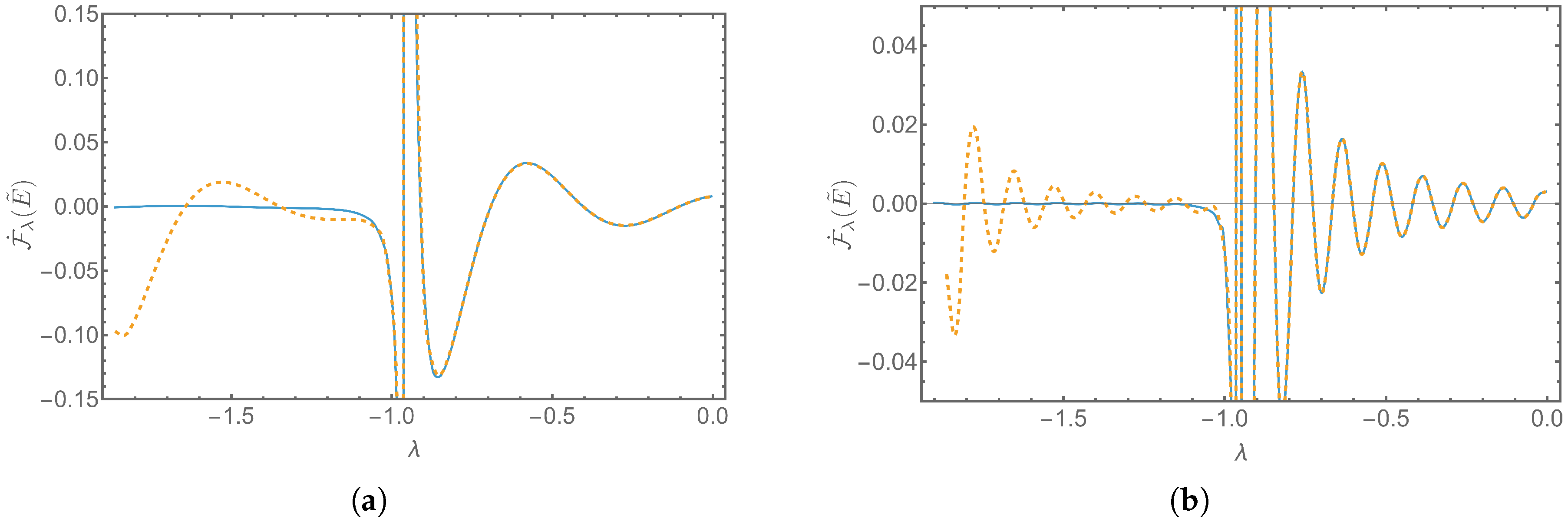
Now that we have described how to accurately and efficiently compute the transition rate for the detector, we need to make one more important parameter determination: the time we turn on the detector, ${\lambda }_{\mathrm{on}}$. An issue we must factor in when providing a time for this parameter is that of transience. Transience describes the junk noise that dominates the detector’s response for a period of time after being turned on, as described in Refs. [20,21,22]; for example. To ensure these effects have subsided, we require the detector to be turned on sufficiently far in the past before we can glean anything physically interesting from the transition rate. Transient noise can be seen in Figure 3, where the orange, dashed curve uses ${\lambda }_{\mathrm{on}}=-2$, and the blue curve uses ${\lambda }_{\mathrm{on}}=-4$. We see that the oscillations occurring before the bounce in these plots are not meaningful representations of the detector’s response to the dynamical gravitational field but transient noise that goes away when ${\lambda }_{\mathrm{on}}$ is pushed further into the past. We found that ${\lambda }_{\mathrm{on}}=-4$ was a reasonable time to switch the detector on for the parameter sets in which we were interested.

4. Results

4.1. MFLE Models

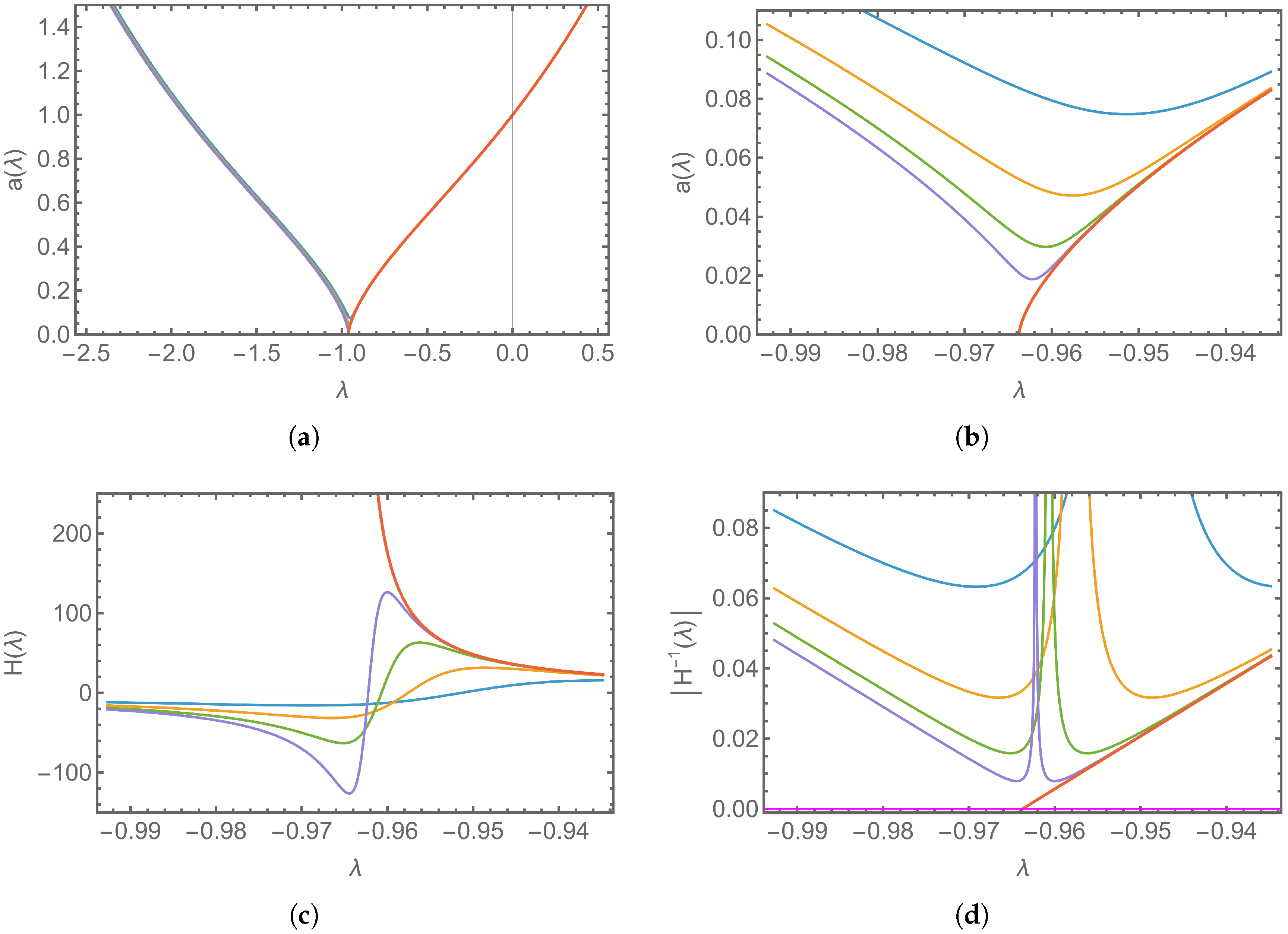
We present in Figure 4 our primary model cosmologies: four unique numerical solutions to the MFLE with varying bounce densities, along with a benchmark Big Bang model using ${\Omega }_b\to \infty$. Sub-figures (a) and (b) showcase only the evolution of the scale factor. Here, we see that at late times, after the Big Bang and outside the bounce region, the MFLE models approach the exact trajectory of the classical Big Bang scale factor. These are the same effects discussed in Section 2 and shown in Figure 2, where introducing a non-zero bounce term has a negligible effect on the cosmology’s scale factor except in regions where radiation is the dominant energy form. We now also see that these regions shift with a change in the bounce density. A model with a high bounce density (purple curve) will not undergo a bounce until the scale factor is sufficiently small, especially in comparison to the blue curve, where the bounce can occur at a lower density and thus at a higher scale factor and a more recent time as well.

Sub-figures (c) and (d) of Figure 4 display the Hubble parameter and Hubble radius, respectively, within the singularity/bounce region. With the Hubble radius, we can think of it as representative of the relative importance of quantum gravity effects. The smaller this quantity is and the closer it evolves towards the Planck length (represented in pink at the bottom of (d)), then more ignoring the quantum effects of gravity becomes a much poorer approximation, and we can no longer justify the assumption that the spacetime is classical. We make note that the Hubble radii of the bouncing models shown in (d) have minima that are much larger in magnitude than the Planck length at their minimum. This justifies our treatment of spacetime as classical at the bounce, notwithstanding the fact that increasing the bounce density results in a smaller minimum in the Hubble radius near the time of the bounce. It follows that in the classical limit ${\Omega }_b\to \infty$, our assumption that spacetime is classical would break down in these regions, and indeed our semi-classical analysis of particle production would also break down. Nonetheless, it is in these areas, where the Hubble radius is at its local minimum and the spacetime is rapidly changing, that we would expect to see increased rates of particle production, particularly for models with a high ${\Omega }_b$ [23].

4.2. Transition Rate Results

With our preliminary bouncing models (Figure 4) and transition rate parameters fully specified—fixing ${\Omega }_m=0.3$, ${\Omega }_r=8.4\ast {10}^{-5}$, ${\Omega }_{\Lambda }=0.7$, ${\lambda }_{\mathrm{on}}=-4$, and leaving ${\Omega }_b$ and $\tilde{E}$ as free parameters—we can now present the detector’s response as it traverses the bouncing cosmology.

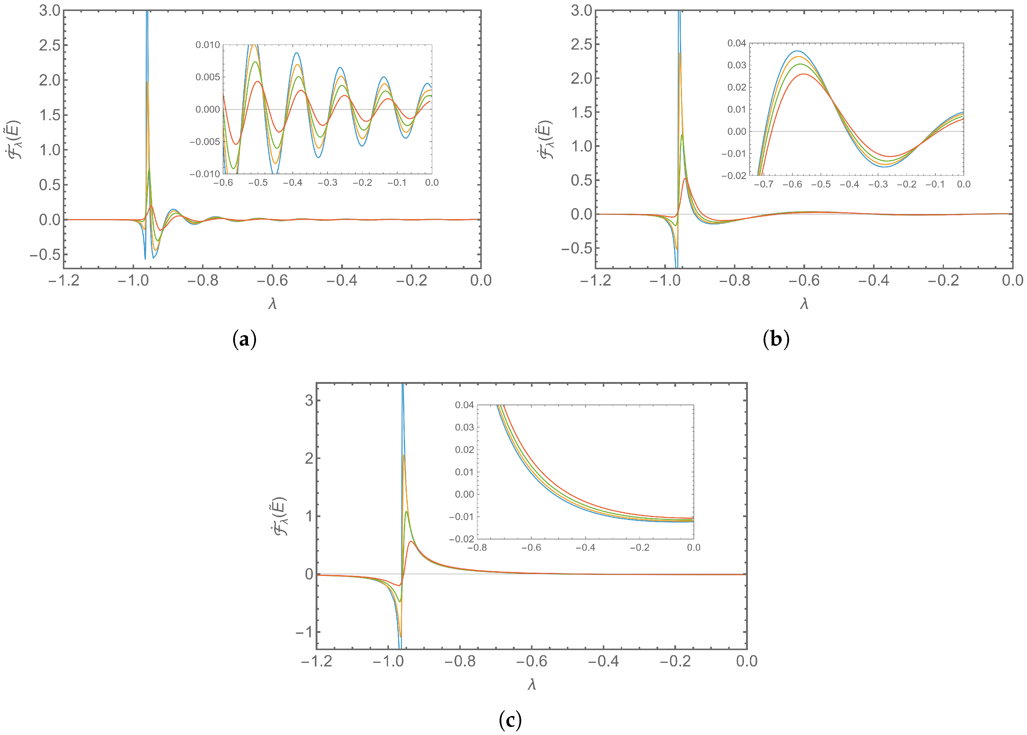
In Figure 5, we show how the transition rate of the Unruh–DeWitt detector varies with ${\Omega }_b$ for three different choices of energy gap. One immediate observation we can make is that the profile of the transition rate after the bounce exhibits damped oscillations with a frequency proportional to the energy gap (or equivalently with a wavelength inversely proportional to the energy gap). For $\tilde{E}=50$ (Figure 5a), we see a very sharp oscillation around the bounce followed by a series of damped oscillations, whereas for $\tilde{E}=1$ (Figure 5c), we find essentially one oscillation around the bounce. For $\tilde{E}=10$ (Figure 5b), there is again a sharp oscillation at the bounce followed by very long-wavelength oscillations. We note also that the amplitudes of the oscillations are inversely proportional to the energy gap. These features were present in the transition rate profiles for the analytical bouncing models studied in Ref. [16].

Looking now at the dependence of the transition rate on the bounce energy density ${\Omega }_b$. Again, we remind the reader that the larger the value of ${\Omega }_b$, the closer the model is to the classical Big Bang singular cosmology and, in particular, the smaller the scale factor at the time of the bounce. We see that the amplitudes of the oscillations seen in the transition rates of the detector are proportional to the bounce density. This relationship is particularly evident in Figure 5a,b, where moving from the blue curve to the red, corresponding to decreasing ${\Omega }_b$, yields noticeably smaller oscillation amplitudes. This relationship between ${\Omega }_b$ and the resulting magnitude of oscillations in the transition rate is a strong signifier for the relative importance of quantum gravity effects near the bounce region that we described in Section 4.1.

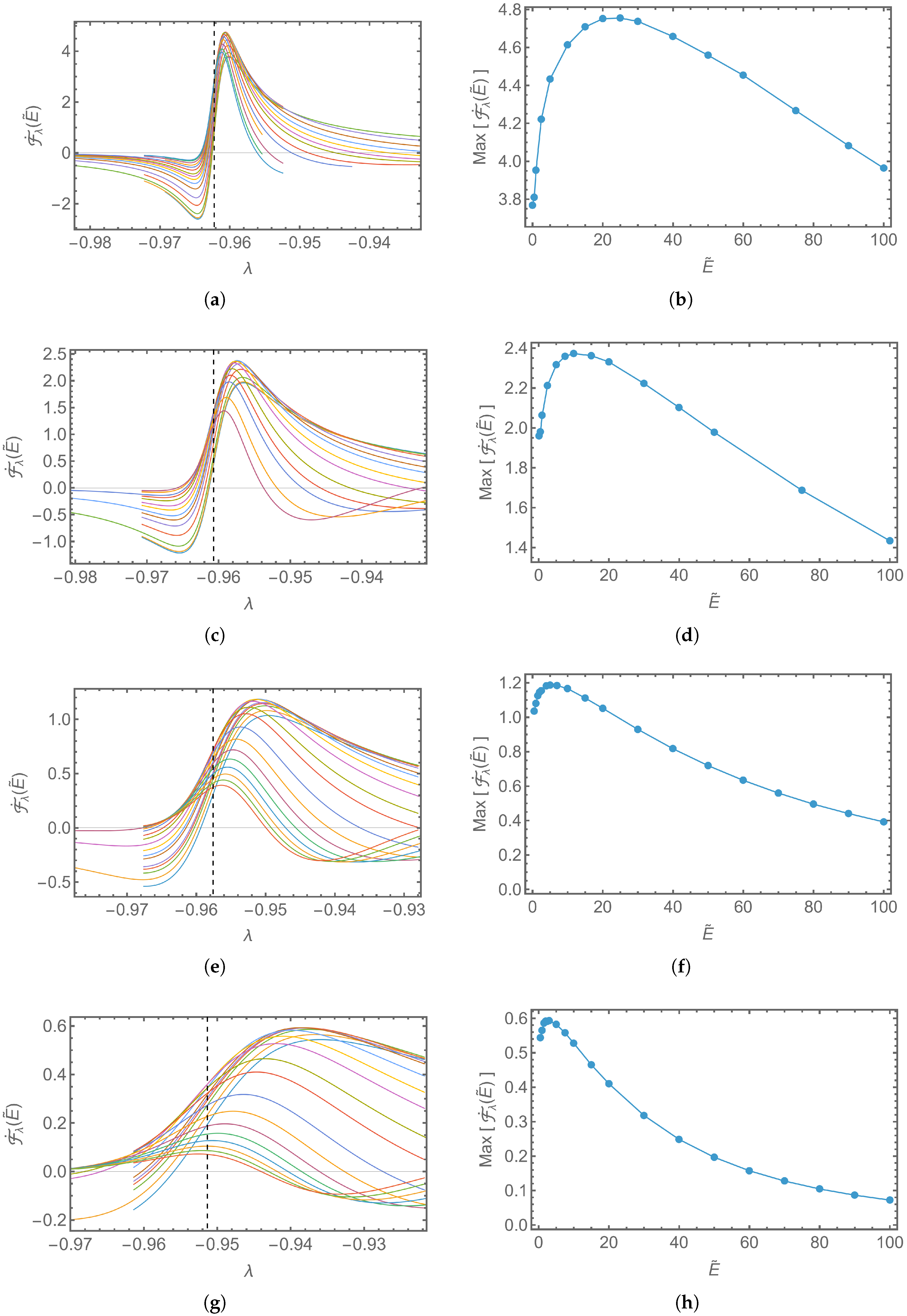
The next set of results that we wish to analyze is the peak detection rate, which occurs just after the bounce. In the analytical models considered in Ref. [16], the peak is inversely proportional to the energy gap. This seems reasonable on physical grounds since it is much less likely that a particle in the ground state will be excited to one in an excited state when the energy gap is large. However, we do not find the relationship quite that straightforward. In Figure 6, each plot in the left column shows the transition rate for a fixed bounce energy density ${\Omega }_b$ with multiple energy gaps. The plots only show the time close to the time of the bounce. In the right column, we plot the peak value of each transition rate curve with its corresponding energy gap. These represent the change in the peak transition rate as a function of energy gap. Interestingly, we find the expected inverse proportionality between the peak of the transition rate and the energy gaps, but only for higher energy gaps. Below some threshold energy level, we find that the peak in the transition rate is actually proportional to the energy gap so that the transition rate increases as the energy gap increases. This is counterintuitive since the transition probability decreases with increased energy gap. The other thing to notice is that the energy threshold where the correlation goes from positive to negative depends on the bounce density, occurring at smaller energy gaps for smaller bounce densities. We notice this in the right column where the turning point, which represents the transition from a positive correlation between the peak of the transition rate and the energy gap to a negative correlation, shifts to smaller values of $\tilde{E}$ as ${\Omega }_b$ decreases. This means that for models closer to the classical singular Big Bang model, there is a large region of the energy gap parameter space where the peak of the transition rate increases with increasing energy gap. As ${\Omega }_b$ gets very small and the spacetime deviates significantly from the standard classical Big Bang model, it is really only very small energy gaps where the peak of the transition rate increases with increasing energy gap. This transition from a region of correlation to anti-correlation in the small energy regime is somewhat reminiscent of the anti-Hawking and anti-Unruh effects observed in Refs. [24,25].

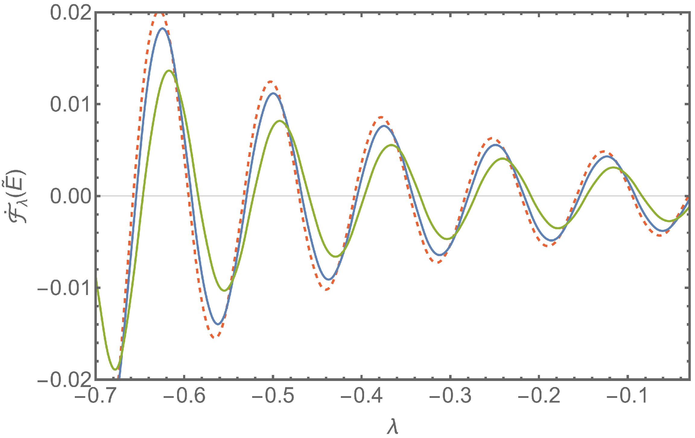
The last case we wish to consider is a comparison between the detector’s response in a bouncing cosmology and a Big Bang cosmology. In what we have considered thus far, we have taken all the models to be bouncing cosmologies and turned the detectors on at some time long before the bounce in order to wash out the transient effects by the time the detector has traversed the bounce. But if we wish to make a direct comparison between a bouncing model and a Big Bang model, then we must turn on the interaction between the quantum field and the detectors at the same time, shortly after the time of the Big Bang in that model. Letting ${\lambda }_{\mathrm{sing}}$ be the dimensionless time of the Big Bang, then we observe the transition rates away from the Big Bang at sufficiently late times to ensure that transience has subsided. In our results, shown in Figure 7, we take ${\lambda }_{\mathrm{on}}={\lambda }_{\mathrm{sing}}+0.001$ and we compare the transition rate of a Big Bang model (${\Omega }_b\to \infty$) with bouncing models corresponding to ${\Omega }_b=1$ and ${\Omega }_b=0.01$. The question we wish to probe is whether there is a late-time signature of the bounce in the Unruh–DeWitt detector. Compared to the Big Bang cosmology (red, dashed curve), the transition rates of the bouncing cosmologies (blue and green curves) have oscillations with amplitudes that are smaller. We expect this because, as described above, a very rapidly varying gravitational field should result in more particle production than a slowly varying gravitational field, and the classical singular model varies more rapidly than any bouncing model near the bounce. For example, even though the bouncing cosmology with ${\Omega }_b=1$ (model shown in blue) varies rapidly near the bounce, it is clear that the gravitational field of the Big Bang model undergoes an even more rapid change there with $\dot{a}\to \infty$ at the singularity.

5. Conclusions

In this work, we investigated semi-classical particle production in non-singular bouncing cosmologies, which are solutions of a modified Friedmann–Lemaître equation (MFLE) derived from LQC. Our aims in this paper were to explore the phenomenology of the solutions to the MFLE and to explore the phenomenology of the response of an Unruh–DeWitt detector propagating in these spacetimes. We had a special interest in the dependence of the detector’s response on the sharpness of the bounce and, in particular, if there remained a “smoking gun” signature of the bounce in the detector’s response at late times.

In our bouncing models, we desired to be as conservative as possible in deviating from the standard $\Lambda$CDM model, and, in particular, we wanted our model to converge to the standard observed model after the radiation-domination epoch. As such, we fixed the energy density parameters at the present epoch to be equal to the benchmark values consistent with the standard $\Lambda$CDM model, with significant deviations from this model occurring only as the radiation domination epoch is approached (running the clock backwards). The deviation is mediated by a bounce density parameter ${\Omega }_b$, which controls both the minimum scale factor at the bounce and the sharpness of the bounce. The background dynamics were obtained by numerically solving the MFLE without invoking piecewise analytic approximations across different energy domination epochs. This ensured that the scale factor and its derivatives remained smooth throughout the entire evolution, eliminating artificial features that can arise in the detector response from gluing approximate solutions.

With our numerical bouncing models obtained, we employed an Unruh–DeWitt particle detector model to explore particle production in these spacetimes. While the Bogoliubov approach to studying cosmological particle production is a very powerful tool, it relies on a global particle definition that is ambiguous in non-asymptotically static cosmologies. Alternatively, the Unruh–DeWitt detector model we utilize here provides a local and operational definition of a particle as an excitation in the energy levels of a localized quantum system interacting with a quantum field. In our analysis, the quantum scalar field that is coupled to the detector is conformally invariant with the field prepared in the conformal vacuum state. While this greatly simplifies the calculations involved, since the Wightman two-point function is known in closed form, it would be interesting to explore the phenomenology for non-conformally invariant fields, either by considering non-conformal coupling or the field in a different quantum state. This is technically a much harder problem since one would require a mode-sum regularization prescription in order to compute the regularized Wightman function, such as those developed in black hole contexts [26,27,28]. We leave this for future work.

Several clear features emerged from our analysis. In agreement with the findings of Ref. [16], we found that after traversing the bounce, the detector exhibits damped oscillations in its transition rate. The oscillation frequency is set by the detector’s energy gap, while the amplitude depends strongly on the bounce density. Sharper bounces—corresponding to larger bounce densities and evolution closer to the classical singular limit—produced higher oscillation amplitudes, reflecting the more rapid variation in the gravitational background. Second, the peak transition rate near the bounce displays nontrivial dependence on the energy gap, while for sufficiently large gaps the peak decreases as the gap increases. We find that below a model-dependent threshold, the peak can instead increase with the energy gap. Finally, by comparing bouncing cosmologies with the classical Big Bang model under identical detector initialization conditions, we found that the singular model produces larger amplitudes in its transition rate oscillations than each of the bouncing models. This is also consistent with our claims that the bounce density dictates these amplitudes, since ${\Omega }_b\to \infty$ in the singular model. The distinction in amplitudes survives into the present epoch, offering a potential signature for whether the universe had a bounce or a bang in its past.

Looking forward, there are several clear avenues of investigation within the scope of this work that we hope to explore further. As already mentioned, it would be very interesting, though technically very challenging, to break the conformal invariance in our model and to explore to what extent any of the features presented here are robust features of the detector’s response in bouncing cosmology, independent of the scalar-curvature coupling or the choice of vacuum state. As well as this, the nontrivial and counterintuitive relationship between the peak transition rate and the detector’s energy gap warrants some further attention. It would be informative to look at this from the perspective of the transition probability rather than the transition rate. The technical challenge there is that the transition probability is divergent in the sharp-switching limit, and so one requires a model for the profile of the switching function. This is not insurmountable, but it adds another degree of complexity to an already challenging numerical computation.

References

1. Lemaître, G. The Beginning of the World from the Point of View of Quantum Theory. Nature 1931, 127, 706. [Google Scholar] [CrossRef]
2. Hubble, E. A Relation between Distance and Radial Velocity among Extra-Galactic Nebulae. Proc. Natl. Acad. Sci. USA 1929, 15, 168–173. [Google Scholar] [CrossRef]
3. Penzias, A.A.; Wilson, R.W. A Measurement of Excess Antenna Temperature at 4080 Mc/s. Astrophys. J. 1965, 142, 419–421. [Google Scholar] [CrossRef]
4. Ijjas, A.; Steinhardt, P.J. Bouncing Cosmology made simple. Class. Quantum Grav. 2018, 35, 135004. [Google Scholar] [CrossRef]
5. Ijjas, A.; Steinhardt, P.J.; Loeb, A. Inflationary schism. Phys. Lett. B 2014, 736, 142–146. [Google Scholar] [CrossRef]
6. Albrecht, A.; Sorbo, L. Can the universe afford inflation? Phys. Rev. D 2004, 70, 063528. [Google Scholar] [CrossRef]
7. Brandenberger, R.; Peter, P. Bouncing Cosmologies: Progress and Problems. Found. Phys. 2017, 47, 797–850. [Google Scholar] [CrossRef]
8. Hawking, S.W.; Ellis, G.F.R. The Large Scale Structure of Space-Time; Cambridge Monographs on Mathematical Physics; Cambridge University Press: Cambridge, UK, 1973. [Google Scholar]
9. Finelli, F.; Brandenberger, R. Generation of a scale-invariant spectrum of adiabatic fluctuations in cosmological models with a contracting phase. Phys. Rev. D 2002, 65, 103522. [Google Scholar] [CrossRef]
10. Brandenberger, R.H. The Matter Bounce Alternative to Inflationary Cosmology. arXiv 2012, arXiv:1206.4196. [Google Scholar] [CrossRef]
11. Ijjas, A.; Steinhardt, P.J. Fully stable cosmological solutions with a non-singular classical bounce. Phys. Lett. B 2017, 764, 289–294. [Google Scholar] [CrossRef]
12. Conroy, A.; Koshelev, A.S.; Mazumdar, A. Defocusing of Null Rays in Infinite Derivative Gravity. J. Cosmol. Astropart. Phys. 2017, 2017, 017. [Google Scholar] [CrossRef][Green Version]
13. Agullo, I.; Singh, P. Loop Quantum Cosmology: A brief review. arXiv 2016, arXiv:1612.01236. [Google Scholar] [CrossRef]
14. Taveras, V. Corrections to the Friedmann equations from loop quantum gravity for a universe with a free scalar field. Phys. Rev. D. 2008, 78, 064072. [Google Scholar] [CrossRef]
15. Rovelli, C.; Wilson-Ewing, E. Why are the effective equations of loop quantum cosmology so accurate? Phys. Rev. D 2014, 90, 023538. [Google Scholar] [CrossRef]
16. Conroy, A.; Taylor, P. Unruh-DeWitt Particle Detectors in Bouncing Cosmologies. arXiv 2024, arXiv:2404.05592. [Google Scholar] [CrossRef]
17. Weinberg, S. Gravitation and Cosmology: Principles and Applications of the General Theory of Relativity; Wiley: New York, NY, USA, 1972. [Google Scholar]
18. Ryden, B. Introduction to Cosmology; Addison-Wesley: Boston, MA, USA, 2002; p. 118. [Google Scholar]
19. Unruh, W.G. Notes on black-hole evaporation. Phys. Rev. D 1976, 14, 870–892. [Google Scholar] [CrossRef]
20. Louko, J.; Satz, A. Transition rate of the Unruh–DeWitt detector in curved spacetime. Class. Quantum Grav. 2008, 25, 055012. [Google Scholar] [CrossRef]
21. Conroy, A. Unruh-DeWitt detectors in cosmological spacetimes. Phys. Rev. D 2022, 105, 123513. [Google Scholar] [CrossRef]
22. Hossain, G.M.; Sardar, G. Transient response from Unruh-DeWitt detector along Rindler trajectory in polymer quantization. arXiv 2017, arXiv:1606.01663. [Google Scholar] [CrossRef]
23. Birrell, N.D.; Davies, P.C.W. Quantum Fields in Curved Space; Cambridge Monographs on Mathematical Physics; Cambridge University Press: Cambridge, UK, 1984. [Google Scholar] [CrossRef]
24. Cozzella, G.; Fulling, S.A.; Landulfo, A.G.S.; Matsas, G.E.A. Uniformly accelerated classical sources as limits of Unruh-DeWitt detectors. Phys. Rev. D 2020, 102, 105016. [Google Scholar] [CrossRef]
25. Robbins, M.P.; Mann, R.B. Anti-Hawking phenomena around a rotating BTZ black hole. Phys. Rev. D 2022, 106, 045018. [Google Scholar] [CrossRef]
26. Taylor, P.; Breen, C. Mode-sum prescription for the vacuum polarization in odd dimensions. Phys. Rev. D 2016, 94, 125024. [Google Scholar] [CrossRef]
27. Taylor, P.; Breen, C. Mode-sum prescription for vacuum polarization in black hole spacetimes in even dimensions. Phys. Rev. D 2017, 96, 105020. [Google Scholar] [CrossRef]
28. Arrechea, J.; Breen, C.; Ottewill, A.; Pisani, L.; Taylor, P. Renormalized stress-energy tensor for scalar fields in the Boulware state with applications to extremal black holes. Phys. Rev. D 2025, 111, 085009. [Google Scholar] [CrossRef]
Figure 1. We plot a variety of model types arising from the classical Friedmann–Lemaître equation. In (a), Big Bang models are shown. The red curve has parameter values { Ω m = 0.3 , Ω r = 8.4 · 10 5 , Ω Λ = 0.7 } with the green, orange, and blue curves having parameter values close to this. Sub-plot (b) shows big bounce models. For reference, the red curve has { Ω m = 0.3 , Ω r = 0.01 , Ω Λ = 0.7 } . Sub-plot (c) shows cyclic models. The red curve has { Ω m = 0.4 , Ω r = 0.025 , Ω Λ = 0.4 } . Sub-plot (d) shows big crunch models. The red curve corresponds to { Ω m = 2 , Ω r = 0.01 , Ω Λ = 0.01 } .
Universe 12 00157 g001
Figure 2. We compare the cosmological evolution between models obeying the classical Friedmann–Lemaître equation (blue, dashed curves) and the MFLE (solid, orange curves). Each sub-figure uses the same density parameter values for both its models, (a) has { Ω m = 0.3 , Ω r = 8.4 · 10 5 , Ω Λ = 0.7 } , (b) has { Ω m = 0 , Ω r = 1 , Ω Λ = 0 } , (c) has { Ω m = 2 , Ω r = 0.01 , Ω Λ = 0 } , and (d) has { Ω m = 0 , Ω r = 0.01 , Ω Λ = 2 } . Each MFLE model shown also uses Ω b = 10 .
Universe 12 00157 g002
Figure 3. We plot the transition rate of the Unruh–DeWitt particle detector to observe transient effects. In (a), both curves use Ω b = 1 and E ˜ = 10 . In (b), both curves use Ω b = 1 and E ˜ = 50 . In both plots, the blue curve is turned on at λ = 4 , and the orange, dashed curve is turned on at λ = 2 .
Universe 12 00157 g003
Figure 4. We plot five MFLE models with varying values of the parameter Ω b . All curves use the benchmark density parameter values. The red curves correspond to the classical Big Bang model, with Ω b = . The blue curves use Ω b = 0.01 , the orange curves use Ω b = 0.1 , the green curves use Ω b = 1 , and the purple curves use Ω b = 10 . In (a), the scale factor is shown for a large region of time. In (b), the scale factor is shown only near the singularity/bounce region. In (c), the Hubble parameter is shown in the bounce region. In (d), the Hubble radius is shown in the bounce region, along with the Planck length represented in pink.
Universe 12 00157 g004
Figure 5. We plot the transition rate of the Unruh–DeWitt particle detector as it traverses the bounce for three energy gaps, E ˜ = 50 in subplot (a), E ˜ = 10 in subplot (b), and E ˜ = 1 in subplot (c). Each subplot has multiple curves corresponding to various Ω b values. In all plots, the blue curve is for Ω b = 10 , the orange curve is for Ω b = 1 , the green curve is for Ω b = 0.1 , and the red curve is for Ω b = 0.01 . The inset in each plot shows the post-bounce evolution enlarged.
Universe 12 00157 g005
Figure 6. In the left column, we plot the transition rates of Unruh–DeWitt particle detectors with varying energy gaps within the bounce region of four different MFLE models. The time of the bounce for each model is displayed with a dashed black line. In the right column, we plot the peak value of each transition rate curve with its corresponding energy gap. Sub-figures (a,b) correspond to Ω b = 10 , (c,d) correspond to Ω b = 1 , (e,f) correspond to Ω b = 0.1 , and (g,h) correspond to Ω b = 0.01 .
Universe 12 00157 g006
Figure 7. We plot the transition rate of the Unruh–DeWitt particle detector to compare the effects of a big bang with a big bounce. Each curve uses λ on = λ sing + 0.001 and E ˜ = 50 . The red, dashed curve shows the transition rate of a detector in a big bang cosmology. The blue and green curves show the transition rate of a detector in a big bounce cosmology, where the green curve uses Ω b = 0.01 and the blue curve uses Ω b = 1 .
Universe 12 00157 g007
Disclaimer/Publisher’s Note: The statements, opinions and data contained in all publications are solely those of the individual author(s) and contributor(s) and not of MDPI and/or the editor(s). MDPI and/or the editor(s) disclaim responsibility for any injury to people or property resulting from any ideas, methods, instructions or products referred to in the content.