Thermodynamics and Phase Transitions of Dyonic AdS Black Holes in Gauss-Bonnet-Scalar Gravity

Abstract

In this paper, by treating the cosmological constant as a thermodynamic pressure, we study the thermodynamics and phase transitions of the dyonic AdS black holes in Gauss-Bonnet-Scalar gravity, where the conformal scalar field is considered. In a more general extended phase space, we first verified the first law of black hole thermodynamics, and find that it is always true. Meanwhile, the corresponding Smarr relation is also obtained. Then, we found that this black hole exhibits interesting critical behaviors in six dimensions, i.e., two swallowtails can be observed simultaneously. Interestingly, in a specific parameter space, we observed the small/intermediate/large black hole phase transitions, with the triple point naturally appearing. Additionally, the small/large black hole phase transition, similar to the liquid/gas phase transition of the van der Waals fluids, can also be found in other parameter regions. Moreover, we note that the novel phase structure composed of two separate coexistence curves discovered in the dyonic AdS black holes in Einstein-Born-Infeld gravity disappears in Gauss-Bonnet-Scalar gravity. This suggests that this novel phase structure may be related to gravity theory, and importantly, it is generally observed that the triple point is a universal property of dyonic AdS black holes. On the other hand, we calculated the critical exponents near the critical points and found that they share the same values as in mean field theory. Finally, it is true that these results will provide some deep insights into the interesting thermodynamic properties of the dyonic AdS black holes in the background of conformal scalar fields.

1. Introduction

The thermodynamics of black holes (BHs) constitutes an important research subject in the field of BH studies. In the 1970s, it was realized that BH is a thermodynamic system with temperature and entropy [1,2,3]. The intriguing thermodynamic properties of BHs are gradually being discovered, which differ from those of ordinary thermodynamic systems. In particular, Hawking and Page discovered a phase transition between stable BHs and thermal radiation, which is referred to as the Hawking-Page phase transition [4]. On the other hand, the anti-de Sitter/conformal field theory (AdS/CFT) correspondence indicates that the thermodynamics of BHs in AdS space can correspond to the thermodynamics of the dual strongly coupled conformal field theory in the boundary of AdS space [5,6,7]. Therefore, in the framework of the AdS/CFT correspondence, the Hawking-Page phase transition is interpreted as a confinement/deconfinement phase transition of gauge fields [8]. Motivated by this inspiration, the thermodynamics and phase transitions of BHs have been widely investigated [9,10,11,12,13,14].

Recently, there has been increasing attention directed towards studying the thermodynamics of AdS BHs in the extended phase space. It is worth noting that, in this framework, the negative cosmological constant $\Lambda$ is interpreted as the thermodynamic pressure, while its conjugate quantity is regarded as the thermodynamic volume [15,16,17,18,19,20,21]. Subsequently, Kubizňák and Mann compared the charged AdS BHs with the van der Waals (vdW) liquid-gas system, and demonstrated that they share the same oscillatory behavior of pressure-volume, critical exponents, and scaling relations [22]. Thus, an analogy between charged AdS BHs and vdW systems has been established. Specifically, the small/large BH phase transition in AdS BHs is similar to the liquid/gas phase transition in vdW fluids. This analogy was applied to different types of AdS BHs, and suggested that such a small/large BH phase transition widely existed [23,24,25,26,27,28]. Later, it was discovered that AdS BHs exhibit more interesting phase transitions in the extended phase space, such as the reentrant phase transition and the triple point [29,30,31,32,33,34,35,36,37,38,39,40,41]. Furthermore, in the context of higher-order Lovelock gravity, there are also some intriguing BHs phase transitions, such as multicritical phase transitions [42,43,44].

By adding higher-order curvature terms to the gravitational action, the extended gravity theories have been established, which include Lovelock gravity and GB gravity [45,46,47]. These extended gravity theories have provided new insights into the study of BHs in higher-dimensional cases. For example, Wei found that charged AdS BHs in GB gravity exhibits small/intermediate/large BH phase transitions in six-dimensional spacetime, with the appearance of triple point [31]. Frassino studied the phase transitions of charged AdS BHs in third-order Lovelock gravity and confirmed the existence of triple point and reentrant phase transitions in higher dimensions [32]. More studies have shown that AdS BHs in extended gravity exhibits many intriguing properties [42,43,44,48,49,50]. On the other hand, quasitopological electromagnetism is a class of interesting and significant objects in the study of BHs [51,52,53,54,55,56]. Recently, Liu et al. have introduced a novel concept of quasitopological electromagnetism, which is defined as the square of the norm of the topological wedge product of the Maxwell field strength of order k ($k>2$) [51]. Subsequently, Li investigated the phase transitions of the dyonic AdS BHs in Einstein-Born-Infeld (EBI) gravity and obtained some interesting results, such as triple point and novel phase structure composed of two separate coexistence curves [57]. Moreover, we also revealed the intriguing thermodynamic properties of dyonic AdS BHs in Einstein-Gauss-Bonnet (EGB) gravity and observed the triple point [58].

Recently, a class of high-dimensional dyonic BH solutions, which include the dyonic BHs in Gauss-Bonnet-Scalar (GBS) gravity, has been derived by coupling Lovelock-Scalar gravity with quasitopological electromagnetism [59]. The conformal scalar field is very important for BHs and it is also quite interesting. Recently, Oliva et al. have developed a model for the gravity theory coupled to the real scalar field [60,61]. Based on this model, higher dimensional BHs with scalar hair have been studied [62,63,64,65,66]. It is believed that the conformal scalar field can affect the thermodynamic stability of hairy BHs [62,63]. Interestingly, one also finds that the conformal scalar field has an impact on the local stability of BHs [59]. Specifically, the range of horizon radius for stable BHs decreases with the increase in the conformal scalar field parameter H. Clearly, these studies indicate that BHs influenced by the conformal scalar field exhibit many intriguing thermodynamic properties which are worthy of further investigation. In addition, although dyonic AdS BHs in EBI gravity and EGB gravity exhibit some rich phase transitions, such as triple points [57,58], it is still unclear whether these intriguing phase transitions also exist in GBS gravity when considering the conformal scalar field. Therefore, in this paper, we study the thermodynamics and phase transitions of the dyonic BHs in GBS gravity by considering the effect of the conformal scalar field in the extended phase space. We are aim to further reveal the interesting thermodynamic properties of the dyonic BHs in GBS gravity and provide insights into the influence of the conformal scalar field on dyonic AdS BHs.

This paper is organized as follows. In Section 2, we give a review of the dyonic BHs in GBS gravity when considering the conformal scalar field. In Section 3, we study the thermodynamics of the dyonic BHs in the extended phase space. In Section 4, we investigate the phase transitions and phase diagrams of the dyonic AdS BHs, where the conformal scalar field is considered. Section 5 involved the computation of critical exponents near the critical points. Finally, Section 6 concludes with a summary and discussion.

2. Review of the Dyonic BHs

The action of high curvature gravity coupled to the conformal scalar field and matter sources can be expressed as [59]

$$\begin{array}{c}\hfill I=\int d^{d}x\sqrt{-g}\left(\sum _{p=0}^{p_{max}}\frac{1}{2^k}{\delta }_{{\sigma }_1{\lambda }_1\cdots {\sigma }_p{\lambda }_p}^{{\mu }_1{\nu }_1\dots {\mu }_p{\nu }_p}\left(a_p{R}_{{\mu }_1{\nu }_1}^{{\sigma }_1{\lambda }_1}\cdots R_{{\mu }_p{\nu }_p}^{{\sigma }_p{\lambda }_p}+b_p{\xi }^{d-4p}{S}_{{\mu }_1{\nu }_1}^{{\sigma }_1{\lambda }_1}\cdots S_{{\mu }_p{\nu }_p}^{{\sigma }_p{\lambda }_p}\right)+{\mathcal{L}}_{qt}\right),\end{array}$$

(1)

where ${\mathcal{L}}_{qt}$ represents the Lagrangian density of matter, $a_p$ is a Lovelock coupling constant, and $b_p$ is a conformal coupling constant. Here, ${\delta }_{{\sigma }_1{\lambda }_1\cdots {\sigma }_p{\lambda }_p}^{{\mu }_1{\nu }_1\cdots {\mu }_p{\nu }_p}$ is the generalized Kronecker delta and $R_{\mu \nu }^{\sigma \lambda }$ represents the components of the Riemann tensor. The tensor $S_{\mu \nu }^{\sigma \lambda }$ is defined as $S_{\mu \nu }^{\sigma \lambda }={\xi }^2{R}_{\mu \nu }^{\sigma \lambda }-2{\delta }_{[\mu }^{[\sigma }{\delta }_{\nu ]}^{\lambda ]}{▿}_{\beta }\xi {▿}^{\beta }\xi -4\xi {\delta }_{[\mu }^{[\sigma }{▿}_{\nu ]}{▿}_{\lambda ]}\xi +8{\delta }_{[\mu }^{[\sigma }{▿}_{\nu ]}\xi {▿}_{\lambda ]}\xi$, where $\xi$ describes the scalar field [60,61]. As a certain class of Lovelock coupling gravity, the dimensionally continued gravity can be obtained when assuming [67,68,69]

$$\begin{array}{c}\hfill a_p=\left(\begin{array}{c}n-1\\ p\end{array}\right)\frac{\left[(d-1)-2p\right]!}{(d-2)!l^{-2(p+1-n)}}.\end{array}$$

(2)

It should be noted that l is related to the cosmological constant, i.e., $\Lambda =-\frac{(d-1)(d-2)}{2l^2}$. Meanwhile, n is associated with the dimensionality parameter d, where $d=2n+1$ is for odd dimensions and $d=2n+2$ is for even dimensions. The gravitational field equation in Equation (1) can be determined by the action principle, i.e.,

$$\begin{array}{c}\hfill \sum _{p=0}^{p_{max}}\frac{a_p}{2^{p+1}}{\delta }_{\beta {\kappa }_1{\rho }_1\cdots {\kappa }_p{\rho }_p}^{\alpha {\sigma }_1{\lambda }_1\dots {\sigma }_p{\lambda }_p}{R}_{{\sigma }_1{\lambda }_1}^{{\kappa }_1{\rho }_1}\cdots R_{{\sigma }_p{\lambda }_p}^{{\kappa }_p{\rho }_p}=-{\varsigma }_{\beta }^{\left(M\right)\alpha }-{\varsigma }_{\beta }^{\left(S\right)\alpha },\end{array}$$

(3)

where ${\varsigma }_{\beta }^{\left(qt\right)\alpha }$ is the energy-momentum tensor corresponding to the material source, and which is defined by

$$\begin{array}{c}\hfill {\varsigma }_{\alpha \beta }^{\left(M\right)}=-\frac{2}{\sqrt{-g}}\frac{\delta I_{qt}}{\delta g^{\alpha \beta }}.\end{array}$$

(4)

One should note that $I_{qt}$ represents the action associated with matter. And, the energy-momentum tensor of the conformal scalar field is

$$\begin{array}{c}\hfill {\varsigma }_{\beta }^{\left(S\right)\alpha }=\sum _{p=0}^{p_{max}}\frac{b_p}{2^{p+1}}{\xi }^{d-4p}{\delta }_{\beta {\kappa }_1{\rho }_1\cdots {\kappa }_p{\rho }_p}^{\alpha {\sigma }_1{\lambda }_1\dots {\sigma }_p{\lambda }_p}{S}_{{\sigma }_1{\lambda }_1}^{{\kappa }_1{\rho }_1}\cdots S_{{\sigma }_p{\lambda }_p}^{{\kappa }_p{\rho }_p}.\end{array}$$

(5)

Based on the action principle, the scalar field equation is constructed as

$$\begin{array}{c}\hfill \sum _{p=0}^{p_{max}}(d-2p)\frac{b_p}{2^p}{\xi }^{(d-1)-4p}{\delta }_{{\kappa }_1{\rho }_1\cdots {\kappa }_p{\rho }_p}^{{\sigma }_1{\lambda }_1\dots {\sigma }_p{\lambda }_p}{S}_{{\sigma }_1{\lambda }_1}^{{\kappa }_1{\rho }_1}\cdots S_{{\sigma }_p{\lambda }_p}^{{\kappa }_p{\rho }_p}=0.\end{array}$$

(6)

Moreover, the Lagrangian density of the material source is

$$\begin{array}{c}\hfill {\mathcal{L}}_{qt}=-\frac{1}{4}{F}_{\rho \sigma }{F}^{\rho \sigma }-\frac{1}{2m!}{H}_{{\nu }_1{\nu }_2\cdots {\nu }_m}{H}^{{\nu }_1{\nu }_2\cdots {\nu }_m}-\eta {\mathcal{L}}_{int},\end{array}$$

(7)

where $\eta$ is a coupling parameter, and ${\mathcal{L}}_{int}$ takes the form of

$$\begin{array}{c}\hfill {\mathcal{L}}_{int}={\delta }_{{\sigma }_1\cdots {\sigma }_d}^{{\rho }_1\cdots {\rho }_d}{F}_{{\rho }_1{\rho }_2}{H}_{{\rho }_3\cdots {\rho }_d}{F}^{{\sigma }_1{\sigma }_2}{H}^{{\sigma }_3\cdots {\sigma }_d}.\end{array}$$

(8)

In addition, the energy-momentum tensor corresponding to the Lagrangian density (7) can be expressed as

$$\begin{array}{cc}\hfill {\varsigma }_{\alpha \beta }^{\left(M\right)}& \hfill =F_{\alpha \rho }{F}_{\beta }^{\rho }-\frac{1}{4}{g}_{\alpha \beta }{F}_{\rho \sigma }{F}^{\rho \sigma }+\frac{1}{2(m-1)!}{H}_{\alpha {\nu }_1\cdots {\nu }_{m-1}}{H}_{\beta }^{{\nu }_1\cdots {\nu }_{m-1}}\hfill \\ \hfill & \hfill -\frac{1}{2{(m!)}^2}{\delta }_{{\sigma }_1\cdots {\sigma }_m\left({\alpha }^{g\beta }\right)\rho }^{{\nu }_1\cdots {\nu }_m\rho }{H}_{{\nu }_1\cdots {\nu }_m}{H}^{{\sigma }_1\cdots {\sigma }_m}+\eta g_{\alpha \beta }{\mathcal{L}}_{int}.\hfill \end{array}$$

(9)

To construct the hairy dyonic BH solutions, one applies condition (2) and the static spherical symmetry line element

$$\begin{array}{c}\hfill d{s}^2=-f\left(r\right)d{t}^2+f{\left(r\right)}^{-1}d{r}^2+r^{2}d{{\rm Y}}_{d-2}^2,\end{array}$$

(10)

where $d{{\rm Y}}_{d-2}^2$ is the metric of the $(d-2)$-dimensional hyper-surface of curvature $(d-2)(d-3)\gamma$, which is defined as

$$\begin{array}{c}\hfill d{{\rm Y}}_{d-2}^2=\left\{\begin{array}{cc}\hfill d{\theta }_1^2+\sum _{j=2}^{d-2}\prod _{l=1}^{j-1}{sin}^2{\theta }_{l}d{\theta }_j^2,\hfill & \hfill \gamma =1,\hfill \\ \hfill d{\theta }_1^2+{sinh}^2{\theta }_{1}d{\theta }_2^2+{sinh}^2{\theta }_1\sum _{j=3}^{d-2}\prod _{l=2}^{j-1}{sin}^2{\theta }_{l}d{\theta }_j^2,\hfill & \hfill \gamma =-1,\hfill \\ \hfill \sum _{j=1}^{d-2}d{\varphi }_j^2,\hfill & \hfill \gamma =0.\hfill \end{array}\right.\end{array}$$

(11)

The magnetic field of this $(d-2)$-dimensional hyper-surface can be expressed as

$$\begin{array}{c}\hfill H_{{\nu }_1{\nu }_2\cdots {\nu }_m}=q\sqrt{\Sigma }{\delta }_{{\nu }_1\cdots {\nu }_m}^{x^1\cdots x^m},\end{array}$$

(12)

where q is related to the magnetic charge and $\Sigma$ represents the volume of the $(d-2)$-dimensional hyper-surface. For the purely electric case, the corresponding Maxwell tensor is of the form

$$\begin{array}{c}\hfill F_{\alpha \beta }=h^{\prime }\left(r\right){\delta }_{\alpha \beta }^{tr},\end{array}$$

(13)

where prime denotes differentiation with respect to r. Based on Equations (12) and (13), the following equation can be obtained,

$$\begin{array}{c}\hfill r^{2(d-2)}\left((d-2)h^{\prime }\left(r\right)+r{h}^{″}\left(r\right)\right)-8\eta {\left((d-2)!\right)}^2{q}^2\left((d-2)h^{\prime }\left(r\right)-r{h}^{″}\left(r\right)\right)=0.\end{array}$$

(14)

Integrating the above equation, it gives

$$\begin{array}{c}\hfill h^{\prime }\left(r\right)=\frac{Q{r}^{d-2}}{r^{2(d-2)}+8\eta {\left((d-2)!\right)}^2{q}^2}.\end{array}$$

(15)

It should be noted that the constant of integration Q in the above equation is related to the electric charge.

The configuration of a scalar field can be defined as

$$\begin{array}{c}\hfill \xi \left(r\right)=\frac{\mathcal{X}}{r}.\end{array}$$

(16)

When the conditions

$$\begin{array}{c}\hfill \sum _{p=0}^{p_{max}}p{b}_p\frac{(d-1)!}{(d-1-2p)!}{\gamma }^{p-1}{\mathcal{X}}^{2-2p}=0,\end{array}$$

(17)

and

$$\begin{array}{c}\hfill \sum _{p=0}^{p_{max}}{b}_p\frac{(d-1)!\left(d(d-1)+4P^2\right)}{(d-1-2p)!}{\gamma }^p{\mathcal{X}}^{-2p}=0\end{array}$$

(18)

are satisfied, it shows that $\xi \left(r\right)$ is a solution of Equation (6). It can be shown that there is an unknown $\mathcal{X}$ in Equations (17) and (18), so that one of these two equations must constitute a constraint on the constant $b_p$’s. Therefore, by considering the gravitational field equations given in Equation (3), choosing the Lovelock parameter $a_p$ arbitrarily, and based on the scalar field $\xi \left(r\right)$ subject to the constraints of Equations (17) and (18), the energy-momentum tensor (9), and (15), an independent equation of motion can be obtained, which takes the form of

$$\begin{array}{cc}\hfill & \hfill \frac{d}{dr}\left[\sum _{p=0}^{p_{max}}{\alpha }_p{\left(\frac{\gamma -f\left(r\right)}{r^2}\right)}^p\right]+\frac{d-1}{r}\sum _{p=0}^{p_{max}}{\alpha }_p{\left(\frac{\gamma -f\left(r\right)}{r^2}\right)}^p\hfill \\ \hfill & \hfill =\frac{q^2}{2(d-2)r^{2d-3}}-\frac{2H}{r^{d+1}}+\frac{Q^2}{2(d-2)\left(r^{2d-3}+8\eta q^2{\left(\Gamma (d-1)\right)}^{2}r\right)},\hfill \end{array}$$

(19)

where

$$\begin{array}{c}\hfill {\alpha }_0=\frac{a_0}{(d-1)(d-2)},{\alpha }_1=1,{\alpha }_p=\prod _{n=3}^{2p}(d-n)a_p\end{array}$$

(20)

with the conditions $p\ge 2$. By solving Equation (19), one obtains

$$\begin{array}{cc}\hfill & \hfill \sum _{p=0}^{p_{max}}{\alpha }_p{\left(\frac{\gamma -f\left(r\right)}{r^2}\right)}^p=\frac{\mu }{r(d-1)}+\frac{2H}{r^d}-\frac{q^2}{2(d-2)(d-3)r^{2(d-2)}}\hfill \\ \hfill & \hfill -\frac{Q^2}{2(d-2)r^{2(d-2)}}{}_{2}F_1\left[1,\frac{d-3}{2(d-2)};\frac{3(d-2)-1}{2(d-2)},\frac{-8\eta q^2{\left(\Gamma (d-1)\right)}^2}{r^{2(d-2)}}\right],\hfill \end{array}$$

(21)

where

$$\begin{array}{c}\hfill H=\sum _{p=0}^{p_{max}}{b}_p\frac{(d-2)!{\gamma }^p{\mathcal{X}}^{d-2p}}{(d-2-2p)!}\end{array}$$

(22)

is a parameter related to the conformal scalar field.

Therefore, by setting ${\alpha }_{0,1,2}\ne 0$ and ${\alpha }_p=0$ for $p\ge 3$ in Equation (21), a spherical ($\gamma =1$)1 dyonic BHs with the effect of conformal scalar field can be obtained in GBS gravity, which is [59]

$$\begin{array}{c}\hfill f\left(r\right)=1+\frac{r^2}{2{\alpha }_2}\left[1-\sqrt{1-\frac{4{\alpha }_2}{l^2}+\frac{8{\alpha }_{2}M}{(d-2)\Sigma r^{d-1}}+\frac{8{\alpha }_{2}H}{r^d}-\frac{8{\alpha }_2{q}^2{r}^{-2(d-2)}}{(d-2)(d-3)}-\frac{2{\alpha }_2{Q}^2\mathcal{F}}{(d-2)r^{2(d-2)}}}\right],\end{array}$$

(23)

where

$$\begin{array}{c}\hfill \mathcal{F}={}_{2}F_1\left[1,\frac{d-3}{2(d-2)};\frac{3(d-2)-1}{2(d-2)};\frac{-8\eta q^2{\left(\Gamma (d-1)\right)}^2}{r^{2(d-2)}}\right]\end{array}$$

(24)

is a hypergeometric function. Here, M is the BH mass, H is the parameter related to the conformal scalar field, $\Sigma$ is the volume of the $(d-2)$-dimensional hyper-surface, and l corresponds to the negative cosmological constant as $\Lambda =-\frac{(d-1)(d-2)}{2l^2}$. Moreover, Q and q represent the electric and magnetic charges of the BH, respectively.

3. Thermodynamics of the Dyonic BHs

In this subsection, we study the thermodynamics of the dyonic BHs in the extended phase space, where the conformal scalar field is considered.In this case, the negative cosmological constant $\Lambda$ is regarded as the thermodynamic pressure $P=-\frac{\Lambda }{8\pi }$ [15]. Furthermore, by solving the equation $f\left(r_h\right)=0$, the outer horizon radius $r_h$ of BH can be obtained, which is determined by the largest root of this equation. Thus, we can express the BH mass in terms of the horizon radius $r_h$ as

$$\begin{array}{cc}\hfill M& \hfill =\frac{q^2{r}_h^{4-d}\Sigma }{4(d-3)r_h}+\frac{8P\pi r_h^{d-1}\Sigma }{d-1}+\frac{(d-2)r_h^{d-5}\Sigma ({\alpha }_2+r_h^2)}{2}-\frac{(d-2)H\Sigma }{r_h}\hfill \\ \hfill & \hfill -{}_{2}F_1\left[1,\frac{d-3}{2(d-2)};\frac{3(d-2)-1}{2(d-2)};\frac{-8\eta q^2{\left(\Gamma (d-1)\right)}^2}{r_h^{2(d-2)}}\right].\hfill \end{array}$$

(25)

Based on the definition of Hawking temperature $T=\frac{f^{\prime }\left(r_h\right)}{4\pi }$, the BH temperature can be determined,

$$\begin{array}{cc}\hfill T& \hfill =\frac{4P\pi r_h^3}{(d-2)(r_h^2+2{\alpha }_2)}+\frac{r_h^{3-d}H}{2\pi (r_h^2+2{\alpha }_2)}+\frac{2(d-1)(r_h^2+{\alpha }_2)}{8\pi r_h(r_h^2+2{\alpha }_2)}-\frac{1}{2\pi r_h}\hfill \\ \hfill & \hfill -\frac{r_h^{7-2d}{q}^2}{8(d-2)\pi (r_h^2+2{\alpha }_2)}-\frac{(d-3)r_h^7{Q}^2}{8(d-2)\pi (r_h^2+2{\alpha }_2)[r_h^{2d}+8r_h^4\eta q^2{(\Gamma (d-1))}^2]}.\hfill \end{array}$$

(26)

Furthermore, in the extended phase space, the BH mass should be regarded as the enthalpy rather than the internal energy, i.e., $\mathcal{H}\equiv M$. Therefore, we can calculate the other thermodynamic quantities of BH, such as the thermodynamic volume V, entropy S, electric potential ${\Phi }_Q$, and magnetic potential ${\Phi }_q$ as follows,

$$\begin{array}{c}\hfill V={\left(\frac{\partial \mathcal{H}}{\partial P}\right)}_{S,Q,q}=\frac{8\pi r_h^{d-1}\Sigma }{d-1},\end{array}$$

(27)

$$\begin{array}{c}\hfill S={\int }_0^{r_h}{T}^{-1}{\left(\frac{\partial \mathcal{H}}{\partial r}\right)}_{P,Q,q}=\frac{2\pi r_h^{d-4}\Sigma \left((d-4)r_h^2+2(d-2){\alpha }_2\right)}{d-4},\end{array}$$

(28)

$$\begin{array}{c}\hfill {\Phi }_Q={\left(\frac{\partial \mathcal{H}}{\partial Q}\right)}_{S,P,q}=\frac{1}{2}Q{r}_h^{3-d}\Sigma {}_{2}F_1\left[1,\frac{d-3}{2(d-2)};\frac{3(d-2)-1}{2(d-2)};\frac{-8\eta q^2{\left(\Gamma (d-1)\right)}^2}{r_h^{2(d-2)}}\right],\end{array}$$

(29)

$$\begin{array}{cc}\hfill {\Phi }_q& \hfill ={\left(\frac{\partial \mathcal{H}}{\partial q}\right)}_{S,P,Q}=\frac{r_h^{3-d}\Sigma q}{2(d-3)}+\frac{(d-3)Q^2{r}_h^{d+3}\Sigma }{4(d-2)q\left[r_h^{2d}+8q^2{r}_h^4\eta {(\Gamma (d-1))}^2\right]}\hfill \\ \hfill & \hfill -\frac{(d-3)r_h^{3-d}{Q}^2\Sigma }{4(d-2)q}{}_{2}F_1\left[1,\frac{d-3}{2(d-2)};\frac{3(d-2)-1}{2(d-2)};\frac{-8\eta q^2{\left(\Gamma (d-1)\right)}^2}{r_h^{2(d-2)}}\right].\hfill \end{array}$$

(30)

Considering the characteristics of the parameters H, ${\alpha }_2$, and $\eta$, we regard them as the new thermodynamic variables. Therefore, it can be verified that these thermodynamic quantities satisfy the follow differential form

$$\begin{array}{c}\hfill d\mathcal{H}=TdS+{\Phi }_{Q}dQ+{\Phi }_{q}dq+{\Phi }_{H}dH+{\Phi }_{{\alpha }_2}d{\alpha }_2+{\Phi }_{\eta }d\eta +VdP,\end{array}$$

(31)

where

$$\begin{array}{c}\hfill {\Phi }_H={\left(\frac{\partial \mathcal{H}}{\partial H}\right)}_{S,P,Q,q,{\alpha }_2,\eta }=-\frac{(d-2)\Sigma }{r_h}\end{array}$$

(32)

is the conjugate quantity to H,

$$\begin{array}{c}\hfill {\Phi }_{{\alpha }_2}={\left(\frac{\partial \mathcal{H}}{\partial {\alpha }_2}\right)}_{S,P,Q,q,H,\eta }=\frac{1}{2}(d-1)r_h^{d-5}\Sigma -\frac{4(d-2)\pi r_h^{d-4}\eta }{d-4}T\end{array}$$

(33)

is the conjugate quantity to ${\alpha }_2$,

$$\begin{array}{cc}\hfill {\Phi }_{\eta }={\left(\frac{\partial \mathcal{H}}{\partial \eta }\right)}_{S,P,Q,q,H,{\alpha }_2}& \hfill =\frac{(d-3)Q^2{r}_h^{3-d}\Sigma }{8(d-2)\eta \left[1+8q^2{r}_h^{4-2d}\eta {(\Gamma (d-1))}^2\right]}-\frac{(d-3)Q^2{r}_h^{3-d}\Sigma }{8(d-2)\eta }\hfill \\ \hfill & \hfill \times {}_{2}F_1\left[1,\frac{d-3}{2(d-2)};\frac{3(d-2)-1}{2(d-2)};\frac{-8\eta q^2{\left(\Gamma (d-1)\right)}^2}{r_h^{2(d-2)}}\right]\hfill \end{array}$$

(34)

is the conjugate quantity to $\eta$. In addition, the corresponding Smarr relation can be obtained, which is of the form

$$\begin{array}{c}\hfill (d-3)\mathcal{H}=(d-2)TS-2PV+(d-3)Q{\Phi }_Q+(d-3)q{\Phi }_q+(d-2)H{\Phi }_H+2{\alpha }_2{\Phi }_{{\alpha }_2}+2\eta {\Phi }_{\eta }.\end{array}$$

(35)

Through the above discussion, we find that both the first law of BH thermodynamics and the Smarr relation hold in a more general extended phase space which H is considered as the new thermodynamic variable.

The Gibbs free energy, as a quantity describing the global stability of a BH system, is given by $G=\mathcal{H}-TS$. Therefore, we obtain

$$\begin{array}{cc}\hfill G& \hfill =\frac{q^2{r}_h^{3-d}\Sigma }{4(d-3)}-\frac{(d-2)H\Sigma }{r_h}+\frac{8P\pi r_h^{d-1}\Sigma }{d-1}+\frac{1}{2}d{r}_h^{d-3}\Sigma +\frac{(d-2)d{r}_h^{d-5}{\alpha }_2\Sigma }{2(d-4)}-\frac{H{r}_h\Sigma }{r_h^2+2{\alpha }_2}\hfill \\ \hfill & \hfill +\frac{q^2{r}_h^{5-d}\Sigma }{4(d-2)(r_h^2+2{\alpha }_2)}-\frac{8P\pi r_h^{d+1}\Sigma }{(d-2)(r_h^2+2{\alpha }_2)}-\frac{(d-1)r_h^{d-1}\Sigma }{2(r_h^2+2{\alpha }_2)}-\frac{2(d-2)H{\alpha }_2\Sigma }{(d-4)r_h(r_h^2+2{\alpha }_2)}\hfill \\ \hfill & \hfill +\frac{r_h^{-1-d}(q^2{r}_h^4-32P\pi r_h^{2d}){\alpha }_2\Sigma }{2(d-4)(r_h^2+2{\alpha }_2)}+\frac{(d-2)(d-1)r_h^{d-5}{\alpha }_2(r_h^2+{\alpha }_2)\Sigma }{(d-4)(r_h^2+2{\alpha }_2)}-\frac{(d-1)r_h^{d-3}{\alpha }_2\Sigma }{2(r_h^2+2{\alpha }_2)}\hfill \\ \hfill & \hfill +\frac{1}{4}{Q}^2{r}_h^{3-d}\Sigma {}_{2}F_1\left[1,\frac{d-3}{2(d-2)};\frac{3(d-2)-1}{2(d-2)};\frac{-8\eta q^2{\left(\Gamma (d-1)\right)}^2}{r_h^{2(d-2)}}\right]\hfill \\ \hfill & \hfill +\frac{(d-3)Q^2{r}_h^{d+3}\Sigma \left((d-4)r_h^2+2(d-2){\alpha }_2\right)}{4(d-4)(d-2)(r_h^2+2{\alpha }_2)\left[r_h^{2d}+8q^2{r}_h^4\eta {\left(\Gamma (d-1)\right)}^2\right]}.\hfill \end{array}$$

(36)

The appearance of a swallowtail in a Gibbs free energy temperature $(G-T)$ diagram indicates the occurrence of a BH phase transition. Therefore, we study BH phase transitions by analyzing the swallowtail observed in the $G-T$ diagram.

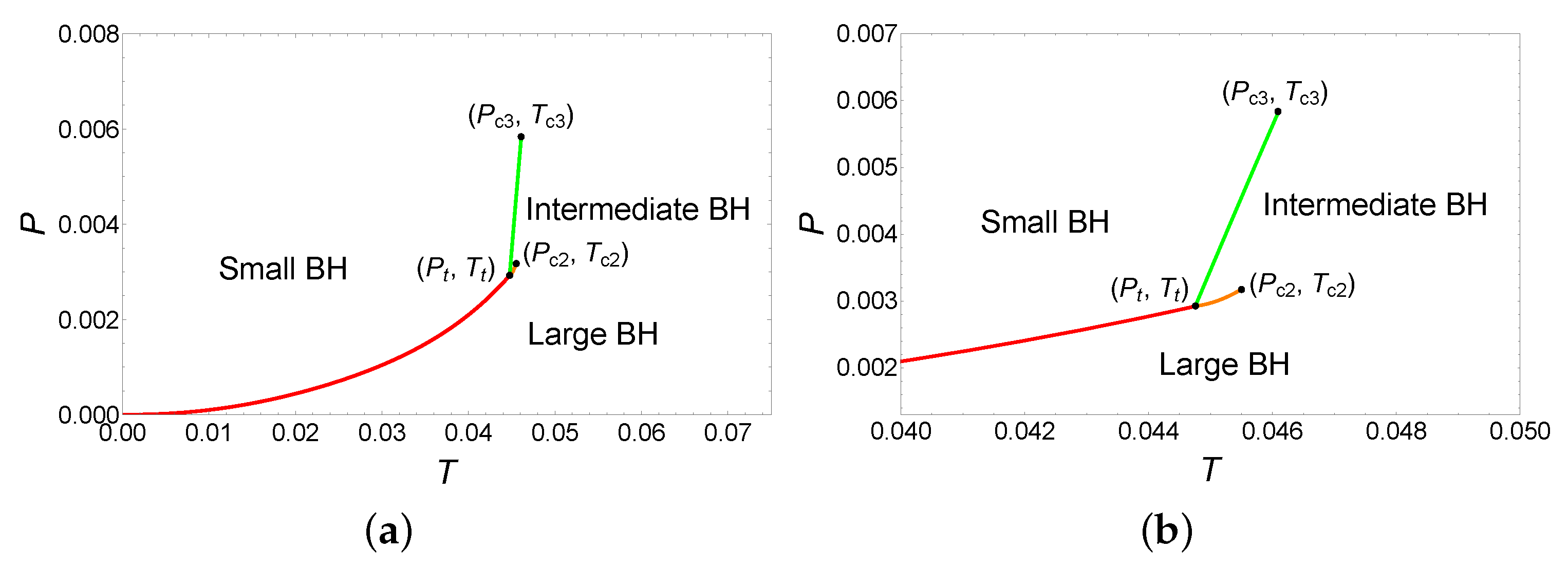
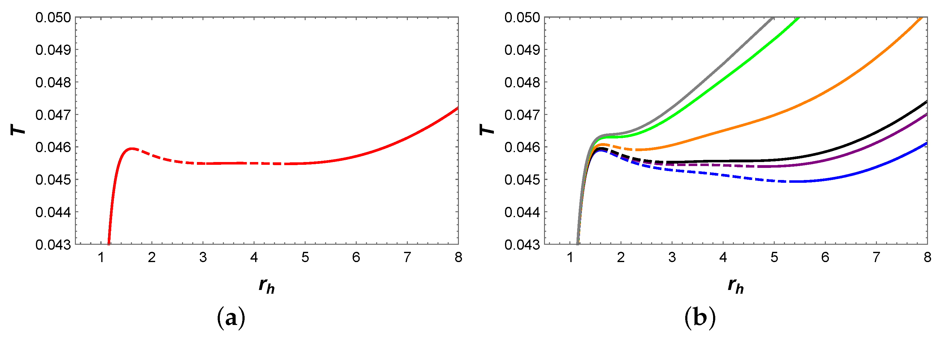
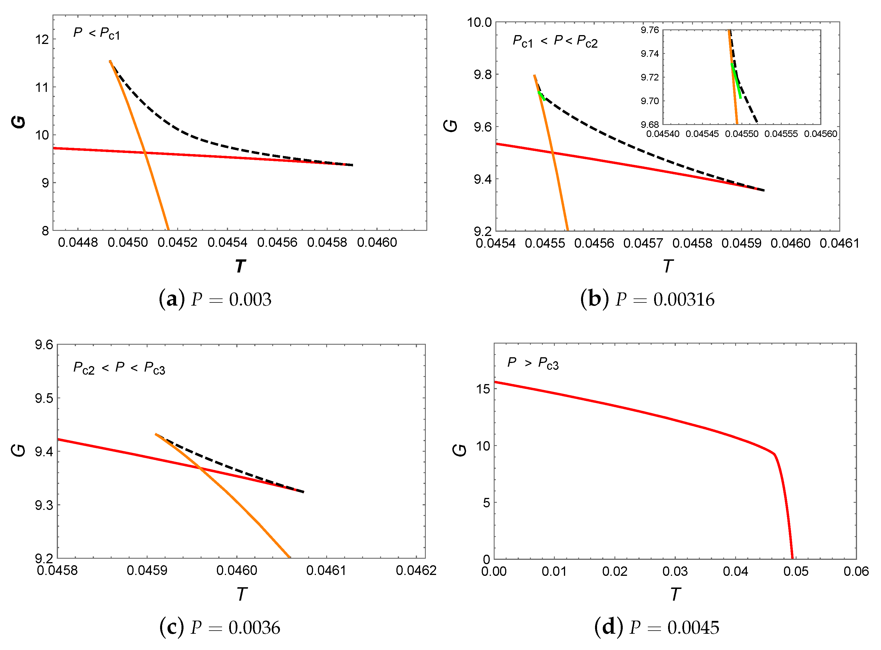
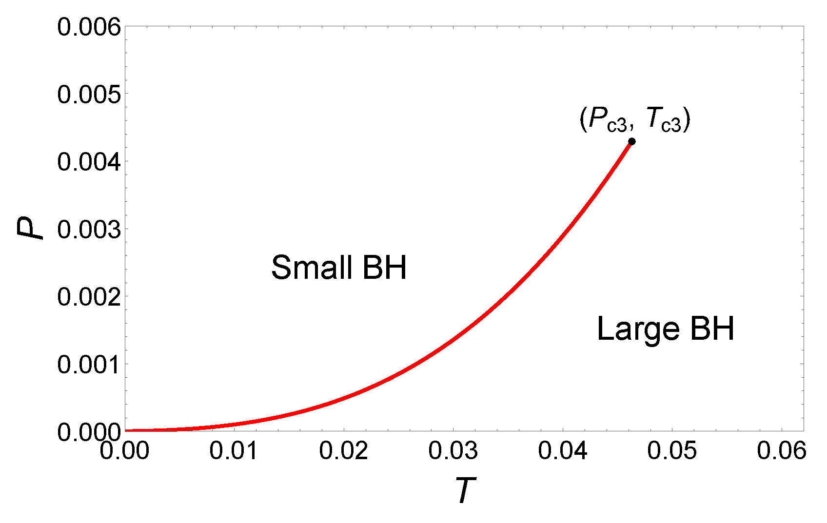
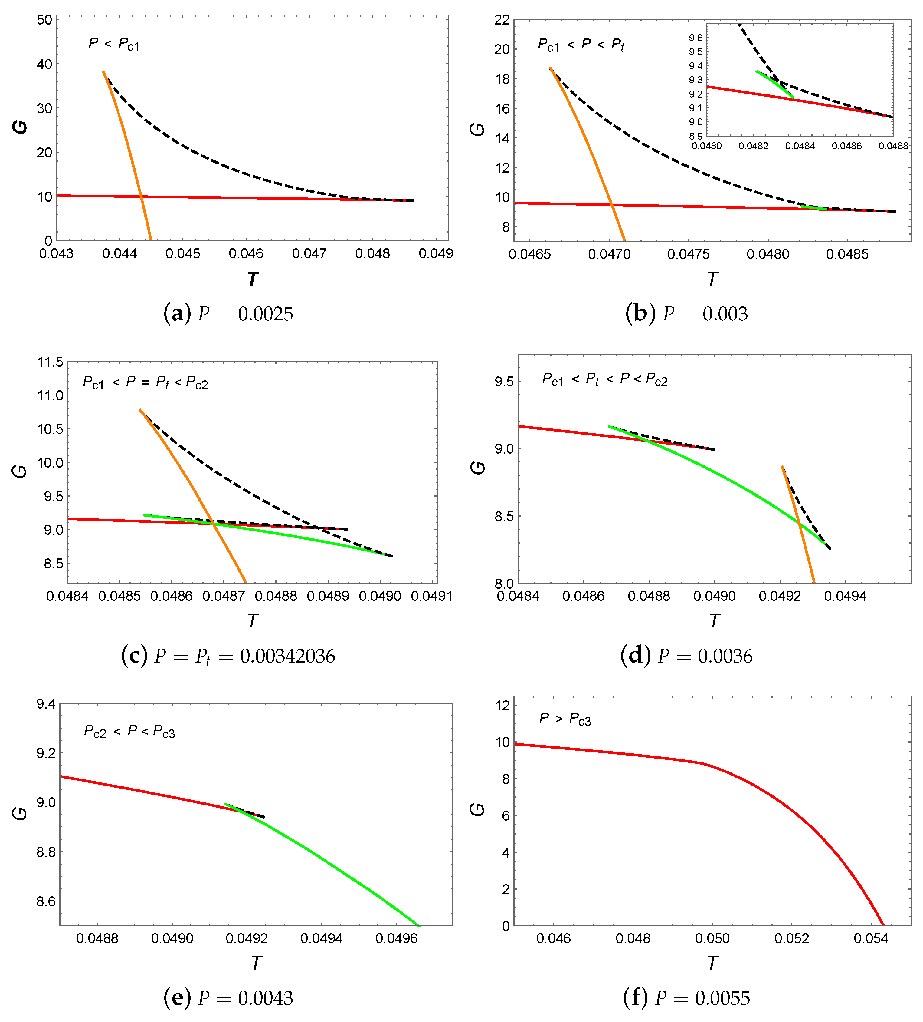
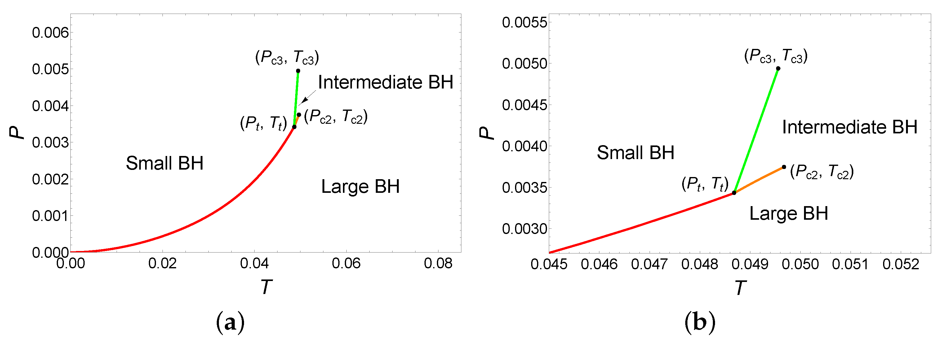
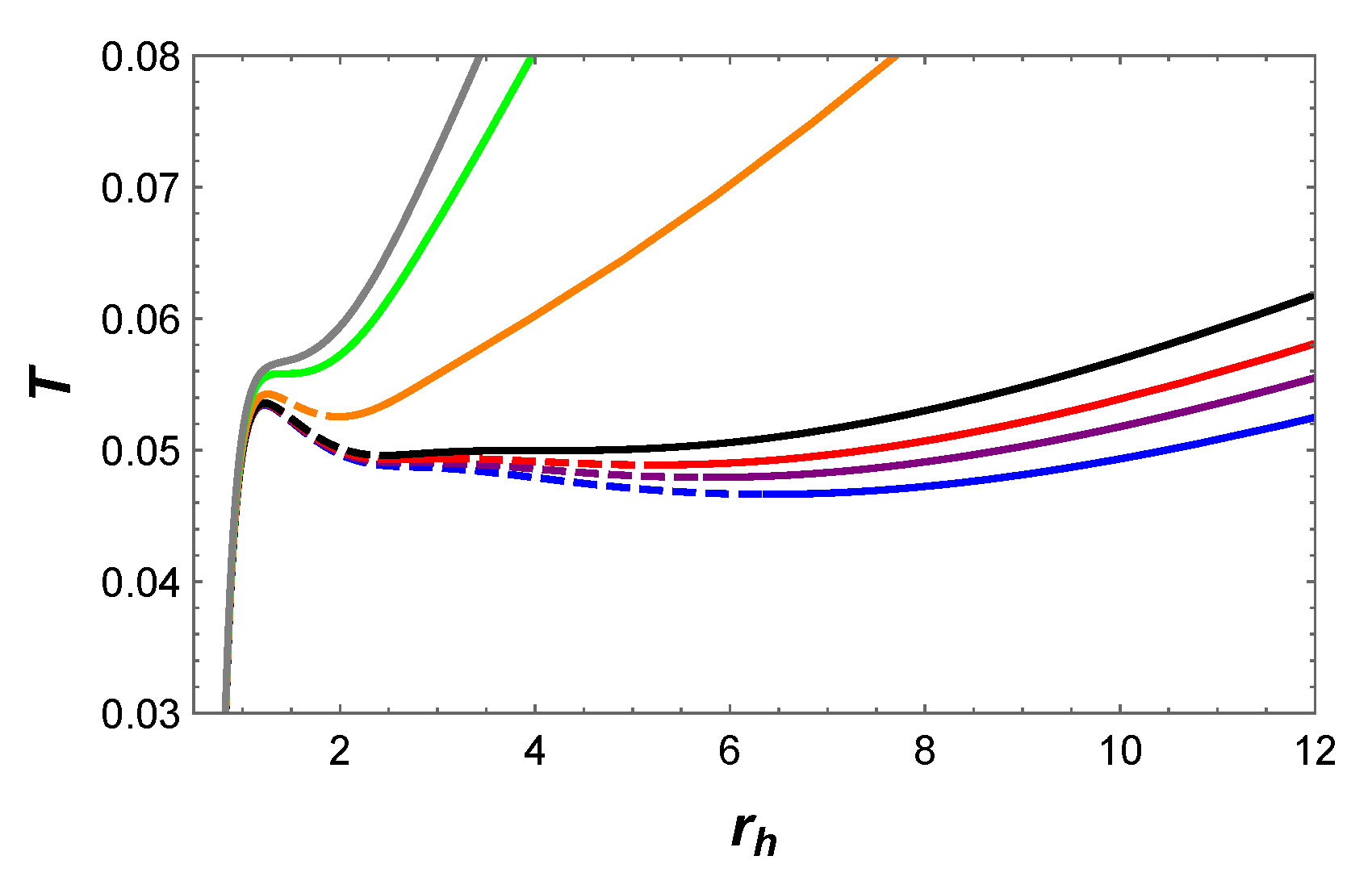
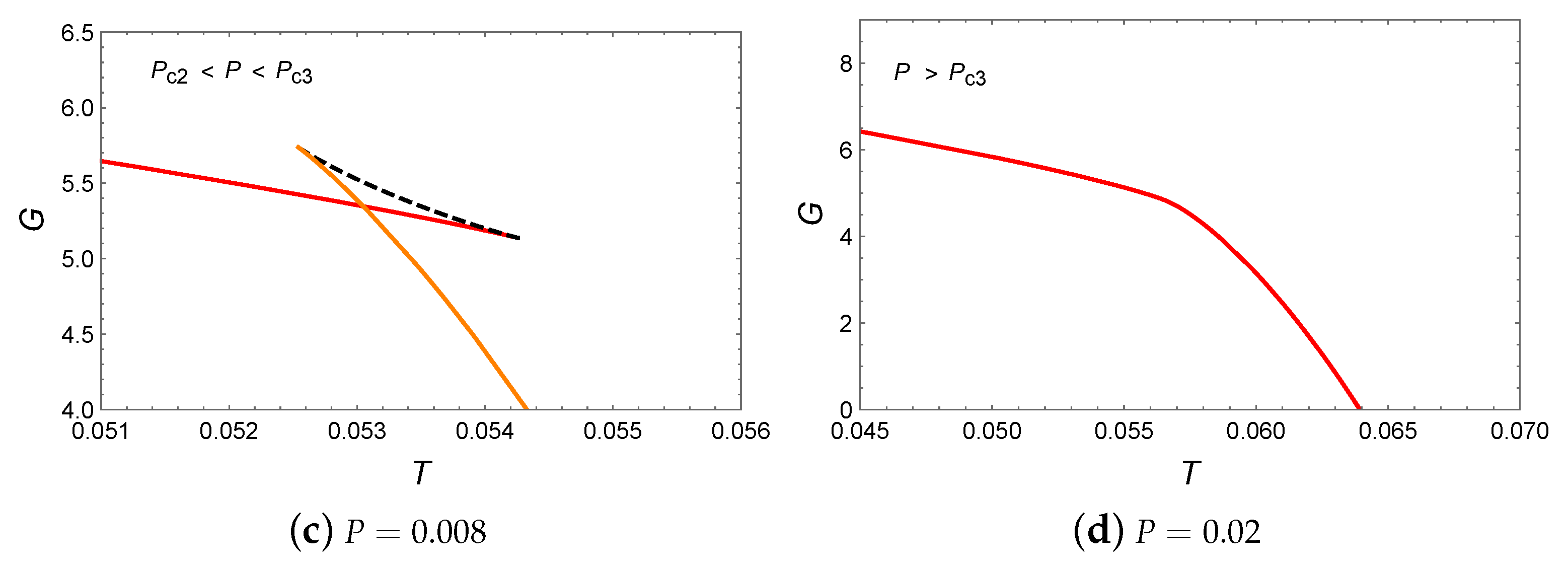
4. Phase Transitions and Phase Diagrams of the Dyonic BHs

In this section, we would like to study the phase transitions and phase diagrams of the dyonic AdS BHs in GBS gravity. In particular, this paper focuses on the BH phase transition in six-dimensional spacetime2. Naturally, based on the temperature Equation (26), the equation of state for the BH can be obtained as

$$\begin{array}{cc}\hfill P(r_h,T)& \hfill =\frac{(d-2)T}{4r_h}+\frac{d-2}{8\pi r_h^2}+\frac{(d-2)T{\alpha }_2}{2r_h^3}+\frac{(d-2){\alpha }_2}{4\pi r_h^4}-\frac{(d-2)H{r}_h^{-d}{\alpha }_2}{4\pi (r_h^2+2{\alpha }_2)}\hfill \\ \hfill & \hfill +\frac{q^2{r}_h^{4-2d}}{32\pi }-\frac{3(d-1)(d-2){\alpha }_2}{16\pi r_h^2(r_h^2+2{\alpha }_2)}-\frac{(d-2)r_h^{-d}\left(2H{r}_h^2+(d-1)r^d\right)}{16\pi (r_h^2+2{\alpha }_2)}\hfill \\ \hfill & \hfill +\frac{(d-3)Q^2{r}_h^4}{32\pi \left[r_h^{2d}+8q^2{r}_h^4\eta {\left(\Gamma (d-1)\right)}^2\right]}-\frac{(d-1)(d-2){\alpha }_2^2}{8\pi r_h^4(r_h^2+2{\alpha }_2)}.\hfill \end{array}$$

(37)

Moreover, considering the thermodynamic volume $V\propto r_h^{d-1}$, the critical point can be determined by the following conditions,

$$\begin{array}{c}\hfill {\left(\frac{\partial P}{\partial r_h}\right)}_T=0,{\left(\frac{{\partial }^{2}P}{\partial r_h^2}\right)}_T=0;or{\left(\frac{\partial T}{\partial r_h}\right)}_P=0,{\left(\frac{{\partial }^{2}T}{\partial r_h^2}\right)}_P=0.\end{array}$$

(38)

As is well known, the local thermodynamic stability of BHs is measured by the heat capacity with a constant pressure, denoted as $C_P$. When $C_P$ is positive, it indicates that the system is locally stable. On the contrary, when $C_P$ is negative, it suggests that the system is locally unstable. For a constant pressure P, the heat capacity $C_P$ is defined as

$$\begin{array}{c}\hfill C_P=T{\left(\frac{\partial S}{\partial T}\right)}_P.\end{array}$$

(39)

By substituting thermodynamic quantities into the calculation, $C_P$ can be further represented as

$$\begin{array}{c}\hfill C_P=T{\left(\frac{{\partial }_{r_h}S}{{\partial }_{r_h}T}\right)}_P\propto {\left({\partial }_{r_h}T\right)}_P^{-1}.\end{array}$$

(40)

In this paper, we follow the conditions of $T>0$ and $S>0$. Thus, in the $T-r_h$ diagram, the BH branches with positive and negative slopes correspond to stable and unstable phases, respectively, and their corresponding $C_P$ values are positive and negative.

Next, we proceed to study BH phase transitions and phase diagrams, with a particular focus on the triple point. In addition, we also focus on the effect of the conformal scalar field on BH phase transitions. Therefore, in this paper, we set the electric charge $Q=10$, magnetic charge $q=5$, and parameter $\Sigma =1$, and vary the conformal scalar field parameter H, the coupling parameters ${\alpha }_2$, and $\eta$ to investigate the phase transitions and phase diagrams of the dyonic BHs.

4.1. Phase Transitions by Fixing H and $\eta$ While Varying ${\alpha }_2$

In this subsection, we study the BH phase transitions and phase diagrams by fixing the conformal scalar field parameter $H=0.01$ and the coupling parameter $\eta =0.01$, while varying ${\alpha }_2$ as 1, 5, and 10.

4.1.1. ${\alpha }_2=1$

In this case, according to Equations (37) and (38), a critical point can be determined, which is

$$\begin{array}{c}\hfill T_c=0.102946, P_c=0.0156174.\end{array}$$

(41)

The behaviors of temperature T with respect to horizon radius $r_h$ and Gibbs free energy G with respect to temperature T are plotted in Figure 1a,b, respectively. It should be noted that isobaric curves of the same color in (a) and (b) correspond to same pressure values. In Figure 1a, when $P<P_c$, two extremal points appear on the isobaric curves (represented by red and green), which divide these two curves into three branches: the stable small BH branch, the unstable intermediate BH branch, and the stable large BH branch. Among them, stable branches are represented by solid curves with a positive value of $C_P$, while unstable branches are represented by dashed curves with a negative value of $C_P$. When $P>P_c$, there is no extremal point on the isobaric curve, and T increases monotonically with $r_h$.

Now, let us focus on the behavior of Gibbs free energy in Figure 1b. For $P<P_c$, a swallowtail appears on each isobaric curve, which suggests the occurrence of a first-order small/large BH phase transition. It should be noted that the nonsmooth points on the isobaric curves in the $G-T$ diagram correspond to the extremal points on the isobaric curves in the $T-r_h$ diagram. Regarding the red and green isobaric curves, it can be found that the system initially exhibits a small BH phase and turns into a large BH phase near the intersection as temperature increases. Furthermore, by comparing the red with the green isobaric curves, it can be discovered that the size of the swallowtail decreases as the pressure increases. When the pressure reaches $P_c$, the swallowtail disappears. For $P>P_c$, the Gibbs free energy decreased monotonically with temperature, which indicates that no phase transition occurs in the system.

The phase diagram for the dyonic BHs, as shown in Figure 1c. It can be observed that the pressure increases monotonically with temperature and terminates at the critical point $(P_c,T_c)$. The region of small BHs is located above the coexistence curve, while the region of large BHs lies below it. This is a typical small/large BH phase transition, which is similar to the vdW liquid/gas phase transition.

4.1.2. ${\alpha }_2=5$

In this case, three critical points can be obtained, which are

$$\begin{array}{c}\hfill T_{c1}=0.0477114, P_{c1}=0.00250879, \end{array}$$

(42)

$$\begin{array}{c}\hfill T_{c2}=0.0496516, P_{c2}=0.00374402, \end{array}$$

(43)

$$\begin{array}{c}\hfill T_{c3}=0.0490982, P_{c3}=0.00444920.\end{array}$$

(44)

Firstly, we focus on the behavior of temperature, as shown in Figure 2a. When $P<P_{c1}$, two extremal points appear on the blue isobaric curve, which divide it into three branches: the stable small BH branch, the unstable intermediate BH branch, and the stable large BH branch. Interestingly, when $P_{c1}<P<P_{c2}$, four extremal points emerged on the red isobaric curve, which divide it into five branches: the stable small BH branch, the unstable small BH branch, the stable intermediate BH branch, the unstable large BH branch, and the stable large BH branch. For $P=P_t=0.00337487$, it is easy to utilize Maxwell equal area laws to construct two pairs of equal area regions in the $T-S$ diagram, as illustrated in Figure 2b. These two pairs of regions have the same temperature, i.e., $T=T_t=0.0485154$. This implies that the BH undergoes two phase transitions simultaneously at such pressure and temperature. In fact, this result indicates the existence of a triple point, where small, intermediate, and large BH phases can coexist. When P increases to $P_{c2}$, the BH system undergoes a second-order BH phase transition. For $P_{c2}<P<P_{c3}$, two extremal points on the orange isobaric curve divide it into three branches: the stable small BH branch, the unstable intermediate BH branch, and the stable intermediate BH branch. Moreover, the first-order phase transition turns to a second-order phase transition as P approaches to $P_{c3}$. When $P>P_{c3}$, the temperature T increases monotonically with $r_h$, which implies that there is only one BH branch.

We have plotted the behavior of Gibbs free energy G with respect to temperature T, as shown in Figure 3. When $P<P_{c1}$, a swallowtail appears in the $G-T$ diagram, which indicates a small/large BH phase transition. As the pressure increased to $P_{c1}<P<P_t$, two swallowtails appear in Figure 3b, which suggests the potential existence of two BH phase transitions. However, the intermediate BH branch is suppressed by the lower free energy branch and does not participate in the phase transition. Therefore, in this case, only the small/large BH phase transition occurs. Increasing the pressure to $P=P_t$, it can be discovered that the intersection points of two swallowtails appear at the same point, which suggests the occurrence of small/intermediate/large BH phase transitions. For $P_t<P<P_{c2}$, two swallowtails can be observed, and all BH branches can participate in the phase transitions. This indicates that in this case, the system can undergo small/intermediate and intermediate/large BH phase transitions simultaneously. When the pressure is increased to $P_{c2}<P<P_{c3}$, one swallowtail can be noticed, which implies that there exists only one small/intermediate BH phase transition. When $P>P_{c3}$, the Gibbs free energy decreases monotonically with temperature, which indicates that no phase transition occurs in the system.

The phase diagram is illustrated in Figure 4, where Figure 4b is a local magnification near the triple point. As can be seen from the phase diagram, the system undergoes the small/large BH phase transition at $P<P_t$. Interestingly, at the triple point ($P_t,T_t$), the small, intermediate, and large BHs phases coexist, and the system undergoes the small/intermediate/large BH phase transitions. When $P_t<P<P_{c2}$, the small/intermediate and intermediate/large BH phase transitions appear simultaneously. When the pressure increases to $P_{c2}<P<P_{c3}$, the system undergoes only the small/intermediate BH phase transition. In summary, these results suggest the presence of a rich variety of phase transition types in this parameter region.

4.1.3. ${\alpha }_2=10$

Similar to the previous case, three critical points are obtained, which are

$$\begin{array}{c}\hfill T_{c1}=0.0349879, P_{c1}=0.0016521, \end{array}$$

(45)

$$\begin{array}{c}\hfill T_{c2}=0.0354822, P_{c2}=0.0019592,\end{array}$$

(46)

$$\begin{array}{c}\hfill T_{c3}=0.0415633, P_{c3}=0.0228754.\end{array}$$

(47)

Firstly, we would like to analyze the behavior of temperature T with respect to $r_h$, as shown in Figure 5. When $P<P_{c1}$, two extremal points appear on the blue isobaric curve, which divide it into three branches: the stable small BH branch, the unstable intermediate BH branch, and the stable large BH branch. As the pressure increases to $P_{c1}<P<P_{c2}$, the red isobaric curve is divided into five branches by four extremal points: the stable small BH branch, the unstable small BH branch, the stable intermediate BH branch, the unstable large BH branch, and the stable large BH branch. For $P_{c2}<P<P_{c3}$, there are two extremal points on the orange isobaric curve, which suggests the existence of three BH branches. When the pressure increases to $P>P_{c3}$, the temperature increases monotonically with $r_h$, which implies that there is only one BH branch.

Next, let us analyze the behavior of Gibbs free energy G with respect to T. When $P<P_{c1}$, the appearance of a swallowtail in Figure 6a actually indicates the small/large BH phase transition. When the pressure increased to $P_{c1}<P<P_{c2}$, two swallowtails can be observed in Figure 6b. However, the intermediate BH branch is suppressed by the BH branches with lower Gibbs free energy and does not participate in the phase transition. Therefore, in this pressure range, only the small/large BH phase transition occurs. For $P_{c2}<P<P_{c3}$, the presence of a swallowtail indicates the occurrence of the small/large BH phase transition. When $P>P_{c3}$, the monotonic decrease in Gibbs free energy suggests that no phase transition occurs in the system.

Finally, the phase diagram is illustrated as shown in Figure 7. The coexistence curve originates from the origin and terminates at the critical point $(P_{c3},T_{c3})$. From the phase diagram, it is evident that while there are three critical points in this parameter region, only the small/large BH phase transitions occur.

4.2. Phase Transitions by Fixing H and ${\alpha }_2$ While Varying $\eta$

In this subsection, by setting the conformal scalar field parameter $H=0.01$ and the coupling parameter ${\alpha }_2=6$, while varying $\eta$ as $0.01$, $0.1$, and 5, we study the BH phase transitions and phase diagrams.

4.2.1. $\eta =0.01$

In this case, three critical points can be obtained, which are

$$\begin{array}{c}\hfill T_{c1}=0.0438641, P_{c1}=0.00209037,\end{array}$$

(48)

$$\begin{array}{c}\hfill T_{c2}=0.0455153, P_{c2}=0.00317372,\end{array}$$

(49)

$$\begin{array}{c}\hfill T_{c3}=0.0460847, P_{c3}=0.00583728.\end{array}$$

(50)

We have plotted the behavior of temperature T with respect to $r_h$, as shown in Figure 8a. For $P_{c1}<P<P_{c2}$, there are four extremal points on the isobaric curve, which suggests the existence of five BH branches. When $P=P_t=0.00292831$, we have utilized Maxwell equal area law to construct two pairs of equal area regions with the same temperature $T=T_t=0.0447573$, as shown in Figure 8b. In fact, this predicts the existence of a triple point. Therefore, we plot the behavior of Gibbs free energy with respect to temperature, as shown in Figure 9. As anticipated, the three BH branches intersect at a point when $P=P_t$, which indicates the occurrence of the small/intermediate/large BH phase transitions. Finally, the phase diagram is plotted in Figure 10. In the phase diagram, the triple point where small, intermediate, and large BHs coexist can be observed.

4.2.2. $\eta =0.1$

Like the previous case, three critical points can be obtained, which are

$$\begin{array}{c}\hfill T_{c1}=0.0454479, P_{c1}=0.00313279,\end{array}$$

(51)

$$\begin{array}{c}\hfill T_{c2}=0.0455649, P_{c2}=0.00319072,\end{array}$$

(52)

$$\begin{array}{c}\hfill T_{c3}=0.0463009, P_{c3}=0.00429228.\end{array}$$

(53)

The $T-r_h$ diagram is illustrated in Figure 11, where four extremal points appear on the red isobaric curve at $P=0.00316$. However, the intermediate BH is suppressed and does not participate in phase transitions, as shown in Figure 12b. This indicates that the system only undergoes the small/large BH phase transitions, similar to the case discussed in Section 4.1.3. Finally, the phase diagram, as illustrated in Figure 13, indicates that only the small/large BH phase transitions occur in this parameter region.

4.2.3. $\eta =5$

In this case, there are three critical points located at

$$\begin{array}{c}\hfill T_{c1}=0.0457980, P_{c1}=0.00324087,\end{array}$$

(54)

$$\begin{array}{c}\hfill T_{c2}=0.0458859, P_{c2}=0.00329751,\end{array}$$

(55)

$$\begin{array}{c}\hfill T_{c3}=0.0463043, P_{c3}=0.00404979.\end{array}$$

(56)

In Figure 14, there exists an isobaric curve with four extremal points, which seems to indicate complex phase transition behavior. However, by analyzing the behavior of Gibbs free energy in Figure 15, it can be found that only the small/large BH phase transitions occur, which is similar to the previous case. The phase diagram in Figure 16 also supports our analysis, which indicates the small/large BH phase transitions occur in this parameter region.

4.3. Phase Transitions by Fixing ${\alpha }_2$ and $\eta$ While Varying H

In this subsection, by setting the coupling parameters ${\alpha }_2=5$ and $\eta =0.01$, while varying the conformal scalar field parameter H as $0.1$ and 1, we study the BH phase transitions and phase diagrams.

4.3.1. $H=0.1$

In this case, three critical points are obtained, i.e.,

$$\begin{array}{c}\hfill T_{c1}=0.0478445, P_{c1}=0.00258937,\end{array}$$

(57)

$$\begin{array}{c}\hfill T_{c2}=0.0496781, P_{c2}=0.00375132,\end{array}$$

(58)

$$\begin{array}{c}\hfill T_{c3}=0.0495021, P_{c3}=0.00494838.\end{array}$$

(59)

The behavior of temperature T with respect to $r_h$ is shown in Figure 17a. For $P_{c1}<P<P_{c2}$, four extremal points appear on each isobaric curve, which indicates a rich variety of phase transitions. Obviously, when $P=P_t=0.00342036$, we have utilized the Maxwell equal area law to construct two pairs of equal area regions, as shown in Figure 17b. Then, we plotted the behavior of Gibbs free energy in Figure 18. In particular, when $P=P_t=0.00342036$, it can be discovered that three BH branches intersect at one point, which suggests the occurrence of small/intermediate/large BH phase transitions. Finally, in the phase diagram shown in Figure 19, a triple point can be observed where small, intermediate, and large BH phases coexist.

4.3.2. $H=1$

Similar to the previous case, three critical points can be obtained, which are

$$\begin{array}{c}\hfill T_{c1}=0.0490380, P_{c1}=0.00326926,\end{array}$$

(60)

$$\begin{array}{c}\hfill T_{c2}=0.0499632, P_{c2}=0.00383222,\end{array}$$

(61)

$$\begin{array}{c}\hfill T_{c3}=0.0558200, P_{c3}=0.01618840.\end{array}$$

(62)

The behaviors of temperature and Gibbs free energy are plotted in Figure 20 and Figure 21. After careful analysis, it can be determined that only small/large BH phase transitions occur in this parameter region. Finally, the phase diagram in Figure 22 further shows this small/large BH phase transition.

5. Critical Exponents

It is widely believed that the critical exponents offer a valuable method for describing the behavior of physical quantities near the critical point, and they do not depend on the details of the physical system. Therefore, in this section we would like to calculate the critical exponents in the vicinity of the critical points.

For convenience, we start by defining some reduced parameters, whereby we set

$$\begin{array}{c}\hfill t=\frac{T}{T_c}-1=\tau -1,\end{array}$$

(63)

where $\tau =\frac{T}{T_c}$ is defined as the reduced thermodynamic temperature, we set

$$\begin{array}{c}\hfill \omega =\frac{V}{V_c}-1=\nu -1,\end{array}$$

(64)

where $\nu =\frac{V}{V_c}$ is defined as the reduced thermodynamic volume, and we define

$$\begin{array}{c}\hfill p=\frac{P}{P_c}\end{array}$$

(65)

as the reduced thermodynamic pressure.

Next, let us review the definitions of the critical exponents $\alpha$, $\beta$, $\gamma$, and $\delta$ near the critical point [22]:

(1)

Exponent $\alpha$ determines the behavior of the specific heat at constant volume,

$$\begin{array}{c}\hfill C_V=T\frac{\partial S}{\partial T}{|}_V\propto {\left|t\right|}^{-\alpha }.\end{array}$$

(66)

(2)

Exponent $\beta$ describes the behavior of the order parameter ${\eta }_1=V_l-V_s$ (the difference between the volumes of the coexisting large and small BHs) on a given isotherm

$$\begin{array}{c}\hfill {\eta }_1=V_l-V_s\propto {\left|t\right|}^{\beta }.\end{array}$$

(67)

(3)

Exponent $\gamma$ governs the behavior of the isothermal compressibility ${\kappa }_T$

$$\begin{array}{c}\hfill {\kappa }_T=-\frac{1}{V}\frac{\partial V}{\partial P}{|}_T\propto {\left|t\right|}^{-\gamma }.\end{array}$$

(68)

(4)

Exponent $\delta$ reflected the following behavior on the critical isotherm $T=T_c$

$$\begin{array}{c}\hfill |P-P_c| \propto |V-V_c{|}^{\delta }.\end{array}$$

(69)

Subsequently, we will proceed to compute these critical exponents. From Equation (28), it can be found that the entropy S is independent of T, which leads

$$\begin{array}{c}\hfill C_V=T\frac{\partial S}{\partial T}{|}_V=0.\end{array}$$

(70)

Thus, the critical exponent is $\alpha =0$.

In addition, by substituting the reduced parameters introduced in Equations (63)–(65) into Equation (37), we can calculate the corresponding state equations. Therefore, it is easy to express the reduced pressure near the critical point as

$$\begin{array}{c}\hfill p=A_0+A_1\omega +A_2{\omega }^2+A_3{\omega }^3+B_{0}t+B_{1}t\omega +\mathcal{O}(t{\omega }^2,{\omega }^4).\end{array}$$

(71)

The values of the expanded coefficients in Equation (71) for different parameters were calculated, and the corresponding results are listed in

Table 1. The values of the expanded coefficients in Equation (71) for different parameters.

H	${\mathit{\alpha }}_2$	$\mathit{\eta }$	${\mathit{A}}_0$	${\mathit{A}}_3$	${\mathit{B}}_0$	${\mathit{B}}_1$
0.01	1	0.01	1	−0.0300092	4.73944	−1.55851
0.01	5	0.01	1	−0.0947391	22.7021	−11.2639
0.01	5	0.01	1	−0.0075045	5.13489	−1.79055
0.01	10	0.01	1	−0.1293810	14.1455	−7.97322
0.01	10	0.01	1	−0.0042004	6.25360	−2.33512
0.01	6	0.01	1	−0.1009740	22.4269	−11.6441
0.01	6	0.01	1	−0.0066289	5.42808	−1.93255
0.01	6	0.1	1	−0.0580844	27.1060	−13.9027
0.01	6	0.1	1	−0.0043064	5.73413	−2.07767
0.01	6	5	1	−0.0597647	28.6375	−14.6833
0.01	6	5	1	−0.0028678	6.79827	−2.60357
0.1	5	0.01	1	−0.0902457	21.6797	−10.8256
0.1	5	0.01	1	−0.0074550	5.15617	−1.80103
1	5	0.01	1	−0.1120780	14.0584	−7.47423
1	5	0.01	1	−0.0068363	5.41632	−1.9295

.

As shown in Table 1, the coefficient $A_0=1$, the coefficient $B_0$ is positive, and the coefficients $A_3$ and $B_1$ are negative. Moreover, the coefficients $A_1$ and $A_2$ are absent in the BH system, and thus they have not been listed in this table. Therefore, the reduced pressure can be re-expressed as

$$\begin{array}{c}\hfill p=1+A_3{\omega }^3+B_{0}t+B_{1}t\omega +\mathcal{O}(t{\omega }^2,{\omega }^4).\end{array}$$

(72)

For a fixed $t<0$, when differentiating the reduced pressure in Equation (72), we obtain

$$\begin{array}{c}\hfill dp=(3A_3{\omega }^2+B_{1}t)d\omega .\end{array}$$

(73)

Additionally, by applying Maxwell equal area law, it can be obtained that

$$\begin{array}{c}\hfill {\int }_{{\omega }_s}^{{\omega }_l}\omega (3A_3{\omega }^2+B_{1}t)d\omega =0,\end{array}$$

(74)

where ${\omega }_s$ and ${\omega }_l$ are the volumes of the coexisting small and large BHs, respectively. Moreover, the coexisting small and large BHs satisfy the following equation of state

$$\begin{array}{c}\hfill p=1+A_3{\omega }_s^3+B_{0}t+B_{1}t{\omega }_s=1+A_3{\omega }_l^3+B_{0}t+B_{1}t{\omega }_l.\end{array}$$

(75)

By solving Equations (74) and (75), we obtain ${\omega }_s=-{\omega }_l=-\sqrt{\frac{B_1}{A_3}}\sqrt{-t}$. Therefore, the order parameter ${\eta }_1$ satisfies the condition

$$\begin{array}{c}\hfill {\eta }_1=V_c({\omega }_l-{\omega }_s)=2V_c\sqrt{\frac{B_1}{A_3}}\sqrt{-t}.\end{array}$$

(76)

Therefore, the exponent $\beta =\frac{1}{2}$.

Then, by differentiating Equation (72), we obtain

$$\begin{array}{c}\hfill \frac{\partial V}{\partial P}{|}_T=\frac{1}{B_1}\frac{V_c}{P_c}\frac{1}{t}+\mathcal{O}\left(\omega \right).\end{array}$$

(77)

Further, we have

$$\begin{array}{c}\hfill {\kappa }_T=-\frac{1}{V}\frac{\partial V}{\partial P}{|}_T\propto -\frac{1}{B_1}\frac{V_c}{P_c}\frac{1}{t},\end{array}$$

(78)

which suggests that the exponent $\gamma =1$.

Lastly, we set the reduced temperature $t=0$ in Equation (72), resulting in

$$\begin{array}{c}\hfill p-1=A_3{\omega }^3,\end{array}$$

(79)

which indicates that the exponent $\delta =3$. Now, it can be verified that these critical exponents satisfy the following scaling laws of thermodynamics, i.e.,

$$\begin{array}{c}\hfill \alpha +2\beta +\gamma =2,\alpha +\beta (1+\delta )=2,\\ \hfill \gamma (1+\delta )=(2-\alpha )(\delta -1),\beta (\delta -1)=\gamma .\end{array}$$

(80)

In summary, these critical exponents near the critical points have been calculated, which are

$$\begin{array}{c}\hfill \alpha =0,\beta =\frac{1}{2},\gamma =1,\delta =3.\end{array}$$

(81)

Therefore, we can conclude that this dyonic BH shares the same critical exponents as the dyonic BH in EBI gravity [57] and EGB gravity [58]. Interestingly, these critical exponents match those in mean field theory. This similarity is of great significance and provides further support for the results obtained in this paper.

6. Conclusions and Discussion

By regarding the cosmological constant as the thermodynamic pressure, we study the thermodynamics and phase transitions of the dyonic AdS BHs in GBS gravity, where the conformal scalar fields are considered. Firstly, we treat the conformal scalar field parameter H and the coupling parameters ${\alpha }_2$ and $\eta$ as novel thermodynamic variables to verify the first law of BH thermodynamics and derive the corresponding Smarr relation in a more general extended phase space. Then, we study the BH phase transitions by analyzing the characteristic behaviors of temperature and Gibbs free energy in six-dimensional spacetime. On the other hand, to analyze the effect of the conformal scalar field on the BH phase transition, we fix and vary the values of the conformal scalar field parameter H and the coupling parameters ${\alpha }_2$ and $\eta$ to study the BH phase transition.

We first consider the case where $H=0.01$ and $\eta =0.01$, while ${\alpha }_2$ takes the values of 1, 5, and 10. For ${\alpha }_2=1$, we observed a typical small/large BH phase transition, which is similar to the vdW liquid/gas phase transition. When ${\alpha }_2=5$, we discovered four extremal points on the isobaric curve in the T-r diagram, as well as two swallowtails in the G-T diagram. This actually indicates a rich variety of phase transitions beyond the small/large BH phase transition. As a result, the small/intermediate/large BH phase transitions can be found in this case. Additionally, the triple point where the small, intermediate, and large BHs can coexist is obtained, i.e., ($P_t=0.00337487,T_t=0.0485154$). For ${\alpha }_2=10$, although there are three critical points, as the intermediate BH branch has a higher free energy and is suppressed by the lower free energy BH branch, thus only the small/large BH phase transition can be discovered. Then, we fixed $H=0.01$ and ${\alpha }_2=6$ while we varied the parameter $\eta$ to study the phase transition of BHs. When $\eta =0.01$, we observed the small/intermediate/large BH phase transitions, as well as the triple point, which is located at ($P_t=0.00292831,T_t=0.0447573$). For the case of $\eta =0.01$ and 5, which is similar to the case of $H=0.01$, $\eta =0.01$, and ${\alpha }_2=10$, only the small/large BH phase transition occurs. Finally, we set ${\alpha }_2=5$ and $\eta =0.01$ and varied the parameter H to study the BH phase transition. For $H=0.1$, the small/intermediate/large BH phase transitions can be found. As expected, a triple point appears, which is located at ($P_t=0.00342036,T_t=0.0486811$). While for $H=1$, only the small/large BH phase transitions can be observed. Based on the above discussions, it can be found that the conformal scalar field has some significant impact on the BH thermodynamics and phase transitions. On the other hand, we also note that the novel phase structure composed of two separate coexistence curves, discovered in EBI gravity [57], is absent in GBS gravity. This is consistent with the results obtained in EGB gravity [58], further suggesting that this novel phase structure is related to the gravity theory. In fact, these results also demonstrate that the triple point, where small, intermediate, and large BHs can coexist, is a universal feature of dyonic AdS BHs.

Moreover, we calculated the critical exponents near the critical points and obtained results for $\alpha =0$, $\beta =\frac{1}{2}$, $\gamma =1$, and $\delta =3$. This implies that these critical exponents share the same values as in mean field theory and are consistent with those obtained in other BH systems. Finally, it can be summarized that our conclusions will provide important insights for a deep understanding of the intriguing thermodynamic properties of the dyonic AdS BHs in GBS gravity.

In addition, holographic duality provides a valuable method for the study of the thermodynamic properties of AdS BHs, i.e., it reveals these characteristics from an alternative perspective [70,71]. Therefore, it is worth utilizing holographic duality to further investigate the thermodynamics of this dyonic AdS BHs, which may reveal more intriguing thermodynamic properties. This will also be a part of our future work.

References

1. Bardeen, J.M.; Carter, B.; Hawking, S.W. The Four laws of black hole mechanics. Commun. Math. Phys. 1973, 31, 161. [Google Scholar] [CrossRef]
2. Bekenstein, J.D. Black holes and entropy. Phys. Rev. D 1973, 7, 2333. [Google Scholar] [CrossRef]
3. Hawking, S.W. Particle Creation by Black Holes. Commun. Math. Phys. 1975, 43, 199, Erratum in Commun. Math. Phys. 1976, 46, 206. [Google Scholar] [CrossRef]
4. Hawking, S.W.; Page, D.N. Thermodynamics of Black Holes in anti-De Sitter Space. Commun. Math. Phys. 1983, 87, 577. [Google Scholar] [CrossRef]
5. Maldacena, J.M. The Large N limit of superconformal field theories and supergravity. Adv. Theor. Math. Phys. 1998, 2, 231. [Google Scholar] [CrossRef]
6. Gubser, S.S.; Klebanov, I.R.; Polyakov, A.M. Gauge theory correlators from noncritical string theory. Phys. Lett. B 1998, 428, 105. [Google Scholar] [CrossRef]
7. Witten, E. Anti-de Sitter space and holography. Adv. Theor. Math. Phys. 1998, 2, 253. [Google Scholar] [CrossRef]
8. Witten, E. Anti-de Sitter space, thermal phase transition, and confinement in gauge theories. Adv. Theor. Math. Phys. 1998, 2, 505. [Google Scholar] [CrossRef]
9. Chamblin, A.; Emparan, R.; Johnson, C.V.; Myers, R.C. Charged AdS black holes and catastrophic holography. Phys. Rev. D 1999, 60, 064018. [Google Scholar] [CrossRef]
10. Chamblin, A.; Emparan, R.; Johnson, C.V.; Myers, R.C. Holography, thermodynamics and fluctuations of charged AdS black holes. Phys. Rev. D 1999, 60, 104026. [Google Scholar] [CrossRef]
11. Surya, S.; Schleich, K.; Witt, D.M. Phase transitions for flat AdS black holes. Phys. Rev. Lett. 2001, 86, 5231. [Google Scholar] [CrossRef]
12. Cho, Y.M.; Neupane, I.P. Anti-de Sitter black holes, thermal phase transition and holography in higher curvature gravity. Phys. Rev. D 2002, 66, 024044. [Google Scholar] [CrossRef]
13. Shen, J.; Wang, B.; Lin, C.Y.; Cai, R.G.; Su, R.K. The phase transition and the Quasi-Normal Modes of black Holes. JHEP 2007, 7, 037. [Google Scholar] [CrossRef]
14. Cai, R.G.; Kim, S.P.; Wang, B. Ricci flat black holes and Hawking-Page phase transition in Gauss-Bonnet gravity and dilaton gravity. Phys. Rev. D 2007, 76, 024011. [Google Scholar] [CrossRef]
15. Kastor, D.; Ray, S.; Traschen, J. Enthalpy and the Mechanics of AdS Black Holes. Class. Quant. Grav. 2009, 26, 195011. [Google Scholar] [CrossRef]
16. Dolan, B.P. Pressure and volume in the first law of black hole thermodynamics. Class. Quant. Grav. 2011, 28, 235017. [Google Scholar] [CrossRef]
17. Cvetic, M.; Gibbons, G.W.; Kubiznak, D.; Pope, C.N. Black Hole Enthalpy and an Entropy Inequality for the Thermodynamic Volume. Phys. Rev. D 2011, 84, 024037. [Google Scholar] [CrossRef]
18. Dolan, B.P.; Kastor, D.; Kubiznak, D.; Mann, R.B.; Traschen, J. Thermodynamic Volumes and Isoperimetric Inequalities for de Sitter Black Holes. Phys. Rev. D 2013, 87, 104017. [Google Scholar] [CrossRef]
19. Kastor, D.; Ray, S.; Traschen, J. Smarr Formula and an Extended First Law for Lovelock Gravity. Class. Quant. Grav. 2010, 27, 235014. [Google Scholar] [CrossRef]
20. Castro, A.; Dehmami, N.; Giribet, G.; Kastor, D. On the Universality of Inner Black Hole Mechanics and Higher Curvature Gravity. JHEP 2013, 7, 164. [Google Scholar] [CrossRef]
21. El-Menoufi, B.M.; Ett, B.; Kastor, D.; Traschen, J. Gravitational Tension and Thermodynamics of Planar AdS Spacetimes. Class. Quant. Grav. 2013, 30, 155003. [Google Scholar] [CrossRef]
22. Kubizňák, D.; Mann, R.B. P-V criticality of charged AdS black holes. JHEP 2012, 7, 33. [Google Scholar] [CrossRef]
23. Gunasekaran, S.; Mann, R.B.; Kubiznak, D. Extended phase space thermodynamics for charged and rotating black holes and Born-Infeld vacuum polarization. JHEP 2012, 11, 110. [Google Scholar] [CrossRef]
24. Chen, S.; Liu, X.; Liu, C.; Jing, J. P-V criticality of AdS black hole in f(R) gravity. Chin. Phys. Lett. 2013, 30, 060401. [Google Scholar] [CrossRef]
25. Cai, R.G.; Cao, L.M.; Li, L.; Yang, R.Q. P-V criticality in the extended phase space of Gauss-Bonnet black holes in AdS space. JHEP 2013, 09, 005. [Google Scholar] [CrossRef]
26. Mo, J.X.; Liu, W.B. Ehrenfest scheme for P-V criticality of higher dimensional charged black holes, rotating black holes and Gauss-Bonnet AdS black holes. Phys. Rev. D 2014, 89, 084057. [Google Scholar] [CrossRef]
27. Zou, D.C.; Liu, Y.; Wang, B. Critical behavior of charged Gauss-Bonnet AdS black holes in the grand canonical ensemble. Phys. Rev. D 2014, 90, 044063. [Google Scholar] [CrossRef]
28. Wei, S.W.; Liu, Y.X. Insight into the Microscopic Structure of an AdS Black Hole from a Thermodynamical Phase Transition. Phys. Rev. Lett. 2015, 115, 111302, Erratum in: Phys. Rev. Lett. 2016, 116, 169903. [Google Scholar] [CrossRef]
29. Altamirano, N.; Kubiznak, D.; Mann, R.B. Reentrant phase transitions in rotating anti–de Sitter black holes. Phys. Rev. D 2013, 88, 101502. [Google Scholar] [CrossRef]
30. Altamirano, N.; Kubizňák, D.; Mann, R.B.; Sherkatghanad, Z. Kerr-AdS analogue of triple point and solid/liquid/gas phase transition. Class. Quant. Grav. 2014, 31, 042001. [Google Scholar] [CrossRef]
31. Wei, S.W.; Liu, Y.X. Triple points and phase diagrams in the extended phase space of charged Gauss-Bonnet black holes in AdS space. Phys. Rev. D 2014, 90, 044057. [Google Scholar] [CrossRef]
32. Frassino, A.M.; Kubiznak, D.; Mann, R.B.; Simovic, F. Multiple Reentrant Phase Transitions and Triple Points in Lovelock Thermodynamics. JHEP 2014, 9, 80. [Google Scholar] [CrossRef]
33. Zhang, M.; Zou, D.C.; Yue, R.H. Reentrant phase transitions and triple points of topological AdS black holes in Born-Infeld-massive gravity. Adv. High Energy Phys. 2017, 2017, 3819246. [Google Scholar] [CrossRef]
34. Dehyadegari, A.; Sheykhi, A. Reentrant phase transition of Born-Infeld-AdS black holes. Phys. Rev. D 2018, 98, 024011. [Google Scholar] [CrossRef]
35. Dehghani, A.; Hendi, S.H.; Mann, R.B. Range of novel black hole phase transitions via massive gravity: Triple points and N-fold reentrant phase transitions. Phys. Rev. D 2020, 101, 084026. [Google Scholar] [CrossRef]
36. Zhang, C.M.; Zou, D.C.; Zhang, M. Triple points and phase diagrams of Born-Infeld AdS black holes in 4D Einstein-Gauss-Bonnet gravity. Phys. Lett. B 2020, 811, 135955. [Google Scholar] [CrossRef]
37. Cui, Y.Z.; Xu, W.; Zhu, B. Hawking-Page transition with reentrance and triple point in Gauss-Bonnet gravity. Phys. Rev. D 2023, 107, 044048. [Google Scholar] [CrossRef]
38. Wei, S.W.; Liu, Y.X. The microstructure and Ruppeiner geometry of charged anti-de Sitter black holes in Gauss–Bonnet gravity: From the critical point to the triple point. Commun. Theor. Phys. 2022, 74, 095402. [Google Scholar] [CrossRef]
39. Liu, Y.P.; Cao, H.M.; Xu, W. Reentrant phase transition with a single critical point of the Hayward-AdS black hole. Gen. Rel. Grav. 2022, 54, 5. [Google Scholar] [CrossRef]
40. Qu, Y.; Tao, J.; Yang, H. Thermodynamics and phase transition in central charge criticality of charged Gauss-Bonnet AdS black holes. Nucl. Phys. B 2023, 992, 116234. [Google Scholar] [CrossRef]
41. Bai, N.C.; Song, L.; Tao, J. Reentrant phase transition in holographic thermodynamicsof Born-Infeld AdS black hole. Eur. Phys. J. C 2024, 84, 43. [Google Scholar] [CrossRef]
42. Tavakoli, M.; Wu, J.; Mann, R.B. Multi-critical points in black hole phase transitions. JHEP 2022, 12, 117. [Google Scholar] [CrossRef]
43. Wu, J.; Mann, R.B. Multicritical phase transitions in multiply rotating black holes. Class. Quant. Grav. 2023, 40, 06LT01. [Google Scholar] [CrossRef]
44. Wu, J.; Mann, R.B. Multicritical phase transitions in Lovelock AdS black holes. Phys. Rev. D 2023, 107, 084035. [Google Scholar] [CrossRef]
45. Lovelock, D. The Einstein tensor and its generalizations. J. Math. Phys. 1971, 12, 498–501. [Google Scholar] [CrossRef]
46. Boulware, D.G.; Deser, S. String Generated Gravity Models. Phys. Rev. Lett. 1985, 55, 2656. [Google Scholar] [CrossRef]
47. Cai, R.G. Gauss-Bonnet black holes in AdS spaces. Phys. Rev. D 2002, 65, 084014. [Google Scholar] [CrossRef]
48. Singh, D.V.; Singh, B.K.; Upadhyay, S. 4D AdS Einstein–Gauss–Bonnet black hole with Yang–Mills field and its thermodynamics. Ann. Phys. 2021, 434, 168642. [Google Scholar] [CrossRef]
49. Bai, N.C.; Li, L.; Tao, J. Topology of black hole thermodynamics in Lovelock gravity. Phys. Rev. D 2023, 107, 064015. [Google Scholar] [CrossRef]
50. Singh, D.V.; Bhardwaj, V.K.; Upadhyay, S. Thermodynamic properties, thermal image and phase transition of Einstein-Gauss-Bonnet black hole coupled with nonlinear electrodynamics. Eur. Phys. J. Plus 2022, 137, 969. [Google Scholar] [CrossRef]
51. Liu, H.S.; Mai, Z.F.; Li, Y.Z.; Lü, H. Quasi-topological Electromagnetism: Dark Energy, Dyonic Black Holes, Stable Photon Spheres and Hidden Electromagnetic Duality. Sci. China Phys. Mech. Astron. 2020, 63, 240411. [Google Scholar] [CrossRef]
52. Cisterna, A.; Giribet, G.; Oliva, J.; Pallikaris, K. Quasitopological electromagnetism and black holes. Phys. Rev. D 2020, 101, 124041. [Google Scholar] [CrossRef]
53. Lei, Y.Q.; Ge, X.H.; Ran, C. Chaos of particle motion near a black hole with quasitopological electromagnetism. Phys. Rev. D 2021, 104, 046020. [Google Scholar] [CrossRef]
54. Cisterna, A.; Henríquez-Báez, C.; Mora, N.; Sanhueza, L. Quasitopological electromagnetism: Reissner-Nordström black strings in Einstein and Lovelock gravities. Phys. Rev. D 2021, 104, 064055. [Google Scholar] [CrossRef]
55. Barrientos, J.; Mena, J. Joule-Thomson expansion of AdS black holes in quasitopological electromagnetism. Phys. Rev. D 2022, 106, 044064. [Google Scholar] [CrossRef]
56. Sekhmani, Y.; Lekbich, H.; Boukili, A.E.; Sedra, M.B. D-dimensional dyonic AdS black holes with quasi-topological electromagnetism in Einstein Gauss–Bonnet gravity. Eur. Phys. J. C 2022, 82, 1087. [Google Scholar] [CrossRef]
57. Li, M.D.; Wang, H.M.; Wei, S.W. Triple points and novel phase transitions of dyonic AdS black holes with quasitopological electromagnetism. Phys. Rev. D 2022, 105, 104048. [Google Scholar] [CrossRef]
58. Mou, P.H.; Jiang, Q.Q.; He, K.J.; Li, G.P. Triple points and phase transitions of D-dimensional dyonic AdS black holes with quasitopological electromagnetism in Einstein-Gauss-Bonnet gravity. arXiv 2023, arXiv:2310.08010. [Google Scholar]
59. Ali, A. Quasitopological electromagnetism, conformal scalar field and Lovelock black holes. Eur. Phys. J. C 2023, 83, 564. [Google Scholar] [CrossRef]
60. Oliva, J.; Ray, S. Conformal couplings of a scalar field to higher curvature terms. Class. Quant. Grav. 2012, 29, 205008. [Google Scholar] [CrossRef]
61. Giribet, G.; Leoni, M.; Oliva, J.; Ray, S. Hairy black holes sourced by a conformally coupled scalar field in D dimensions. Phys. Rev. D 2014, 89, 085040. [Google Scholar] [CrossRef]
62. Giribet, G.; Goya, A.; Oliva, J. Different phases of hairy black holes in AdS5 space. Phys. Rev. D 2015, 91, 045031. [Google Scholar] [CrossRef]
63. Galante, M.; Giribet, G.; Goya, A.; Oliva, J. Chemical potential driven phase transition of black holes in anti–de Sitter space. Phys. Rev. D 2015, 92, 104039. [Google Scholar] [CrossRef]
64. Hennigar, R.A.; Tjoa, E.; Mann, R.B. Thermodynamics of hairy black holes in Lovelock gravity. JHEP 2017, 2, 70. [Google Scholar] [CrossRef]
65. Dykaar, H.; Hennigar, R.A.; Mann, R.B. Hairy black holes in cubic quasi-topological gravity. JHEP 2017, 5, 45. [Google Scholar] [CrossRef]
66. Chernicoff, M.; Fierro, O.; Giribet, G.; Oliva, J. Black holes in quasi-topological gravity and conformal couplings. JHEP 2017, 2, 10. [Google Scholar] [CrossRef]
67. Kuang, X.M.; Miskovic, O. Thermal phase transitions of dimensionally continued AdS black holes. Phys. Rev. D 2017, 95, 046009. [Google Scholar] [CrossRef]
68. Ali, A.; Saifullah, K. Magnetized topological black holes of dimensionally continued gravity. Phys. Rev. D 2019, 99, 124052. [Google Scholar] [CrossRef]
69. Ali, A. Magnetized hairy black holes of dimensionally continued gravity coupled to double-logarithmic electrodynamics. Eur. Phys. J. Plus 2022, 137, 108. [Google Scholar] [CrossRef]
70. Ahmed, M.B.; Cong, W.; Kubizňák, D.; Mann, R.B.; Visser, M.R. Holographic Dual of Extended Black Hole Thermodynamics. Phys. Rev. Lett. 2023, 130, 181401. [Google Scholar] [CrossRef]
71. Ahmed, M.B.; Cong, W.; Kubiznak, D.; Mann, R.B.; Visser, M.R. Holographic CFT phase transitions and criticality for rotating AdS black holes. JHEP 2023, 8, 142. [Google Scholar] [CrossRef]
Figure 1. (a) Temperature T vs. horizon radius r h . (b) Gibbs free energy G vs. temperature T. The red, green, orange, and black isobaric curves in (a,b) correspond to P = 0.01 , 0.013 , 0.0156174 , and 0.02 , respectively. Solid curves indicate stable branches, while dashed curves represent unstable branches. (c) P-T phase diagram for the six-dimensional dyonic BHs when H = 0.01 , η = 0.01 and α 2 = 1 .
Universe 10 00087 g001
Figure 2. (a) T vs. r h . The blue, red, black, orange, green and gray curves correspond to P = 0.0024 , 0.00337487 , 0.00374402 , 0.004 , 0.0044492 and 0.005 , respectively. Solid curves indicate stable branches, while dashed curves represent unstable branches. (b) T S diagram of two pairs of equal area regions at pressure P = P t = 0.00337487 . The horizontal line has a temperature T = T t = 0.0485154 .
Universe 10 00087 g002
Figure 3. G vs. T. The red, green and orange curves represent the small, intermediate and large BHs, while the dashed curves indicate unstable BHs.
Universe 10 00087 g003aUniverse 10 00087 g003b
Figure 4. Phase diagram for the six-dimensional dyonic BHs with H = 0.01 , η = 0.01 and α 2 = 5 . (a) Entire phase diagram. (b) An enlarged view near the triple point ( P t , T t ).
Universe 10 00087 g004
Figure 5. (a) T vs. r h for P = 0.0019 . (b) T vs. r h , where the blue, purple, black, orange, green and gray curves represent P = 0.0015 , 0.0016521 , 0.0019592 , 0.01 , 0.0228754 and 0.03 , respectively. Solid curves indicate stable branches, while dashed curves represent unstable branches.
Universe 10 00087 g005
Figure 6. G vs. T. The red, green and orange curves represent the small, intermediate and large BHs, while the dashed curves indicate unstable BHs.
Universe 10 00087 g006
Figure 7. Phase diagram for the six-dimensional dyonic BHs with H = 0.01 , η = 0.01 and α 2 = 10 .
Universe 10 00087 g007
Figure 8. (a) T vs. r h . The blue, red, black, orange, green, and gray curves correspond to P = 0.002 , 0.00292831 , 0.00317372 , 0.004 , 0.00583728 , and 0.007 , respectively. The solid and dashed curves represent stable and unstable branches, respectively. (b) T S diagram of two pairs of equal area regions at a pressure of P = P t = 0.00292831 . The horizontal line has a temperature of T = T t = 0.0447573 .
Universe 10 00087 g008
Figure 9. G vs. T. The red, green and orange curves represent the small, intermediate and large BHs, while the dashed curves indicate unstable BHs.
Universe 10 00087 g009
Figure 10. Phase diagram for the six-dimensional dyonic AdS BHs with H = 0.01 , α 2 = 6 , and η = 0.01 . (a) Entire phase diagram. (b) An enlarged view near the triple point ( P t , T t ).
Universe 10 00087 g010
Figure 11. (a) T vs. r h for P = 0.00316 . (b) T vs. r h , where the blue, purple, black, orange, green, and gray curves represent P = 0.003 , 0.00313279 , 0.00319072 , 0.0036 , 0.00429228 , and 0.0045 , respectively. The solid and dashed curves represent stable and unstable branches, respectively.
Universe 10 00087 g011
Figure 12. G vs. T. The red, green, and orange curves represent the small, intermediate, and large BHs, while the dashed curves indicate unstable BHs.
Universe 10 00087 g012
Figure 13. Phase diagram for the six-dimensional dyonic BHs with H = 0.01 , α 2 = 6 , and η = 0.1 .
Universe 10 00087 g013
Figure 14. (a) T vs. r h for P = 0.00327 . (b) T vs. r h , where the blue, purple, black, orange, green, and gray curves represent P = 0.003 , 0.00324087 , 0.00329751 , 0.0036 , 0.00404979 , and 0.0045 , respectively. The solid and dashed curves represent stable and unstable branches, respectively.
Universe 10 00087 g014
Figure 15. G vs. T. The red, green and orange curves represent the small, intermediate and large BHs, while the dashed curves indicate unstable BHs.
Universe 10 00087 g015aUniverse 10 00087 g015b
Figure 16. Phase diagram for the six-dimensional dyonic AdS BHs with H = 0.01 , α 2 = 6 and η = 5 .
Universe 10 00087 g016
Figure 17. (a) T vs. r h . The blue, red, black, orange, green, and gray curves corresponds to P = 0.0025 , 0.00342036 , 0.00375132 , 0.0043 , 0.00494838 , and 0.0055 , respectively. The solid and dashed curves represent stable and unstable branches, respectively. (b) T S diagram of two pairs of equal area regions at pressure P = P t = 0.00342036 . The horizontal line has a temperature T = T t = 0.0486811 .
Universe 10 00087 g017
Figure 18. G vs. T. The red, green, and orange curves represent the small, intermediate, and large BHs, while the dashed curves indicate unstable BHs.
Universe 10 00087 g018
Figure 19. Phase diagram for the six-dimensional dyonic AdS BHs with α 2 = 5 , η = 0.01 , and H = 0.1 . (a) Entire phase diagram. (b) An enlarged view near the triple point ( P t , T t ).
Universe 10 00087 g019
Figure 20. T vs. r h , where the blue, purple, red, black, orange, green, and gray curves represent P = 0.003 , 0.00326926 , 0.0035 , 0.00383222 , 0.008 , 0.0161884 , and 0.02 , respectively. The solid and dashed curves represent stable and unstable branches, respectively.
Universe 10 00087 g020
Figure 21. G vs. T. The red, green and orange curves represent the small, intermediate and large BHs, while the dashed curves indicate unstable BHs.
Universe 10 00087 g021aUniverse 10 00087 g021b
Figure 22. Phase diagram for the six-dimensional dyonic AdS BHs with α 2 = 5 , η = 0.01 , and H = 1 .
Universe 10 00087 g022