
Mapping LULC Dynamics and Its Potential Implication on Forest Cover in Malam Jabba Region with Landsat Time Series Imagery and Random Forest Classification

 ,
,
Abstract
1. Introduction
2. Materials and Methods
2.1. Study Area
2.2. Data Acquisition
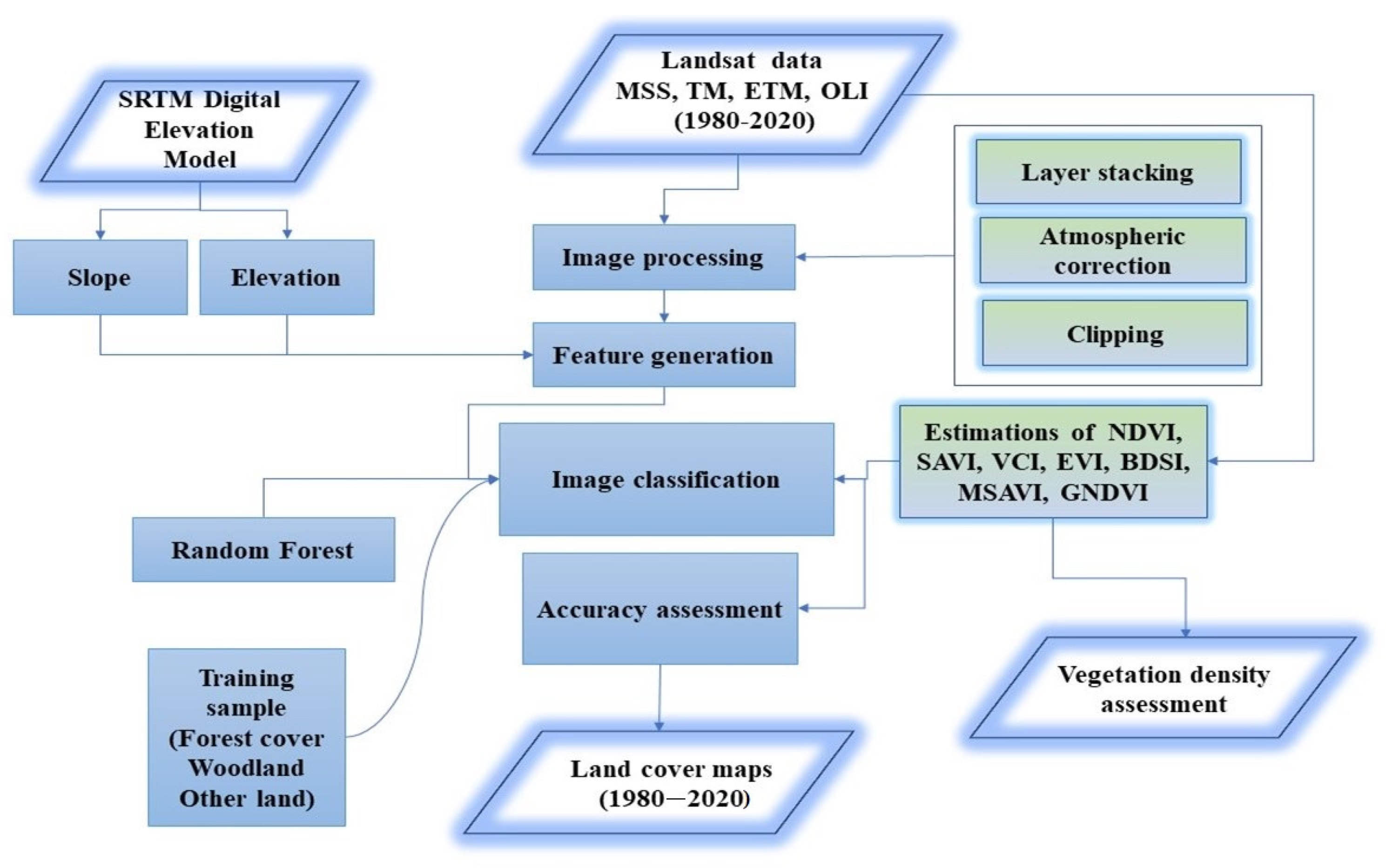
2.3. Satellite Data Processing
2.4. Feature Generation
2.5. Image Classification Processing
2.6. Random Forest Classification Processing
2.7. Accuracy Assessment
2.8. Training and Validation Data
3. Results
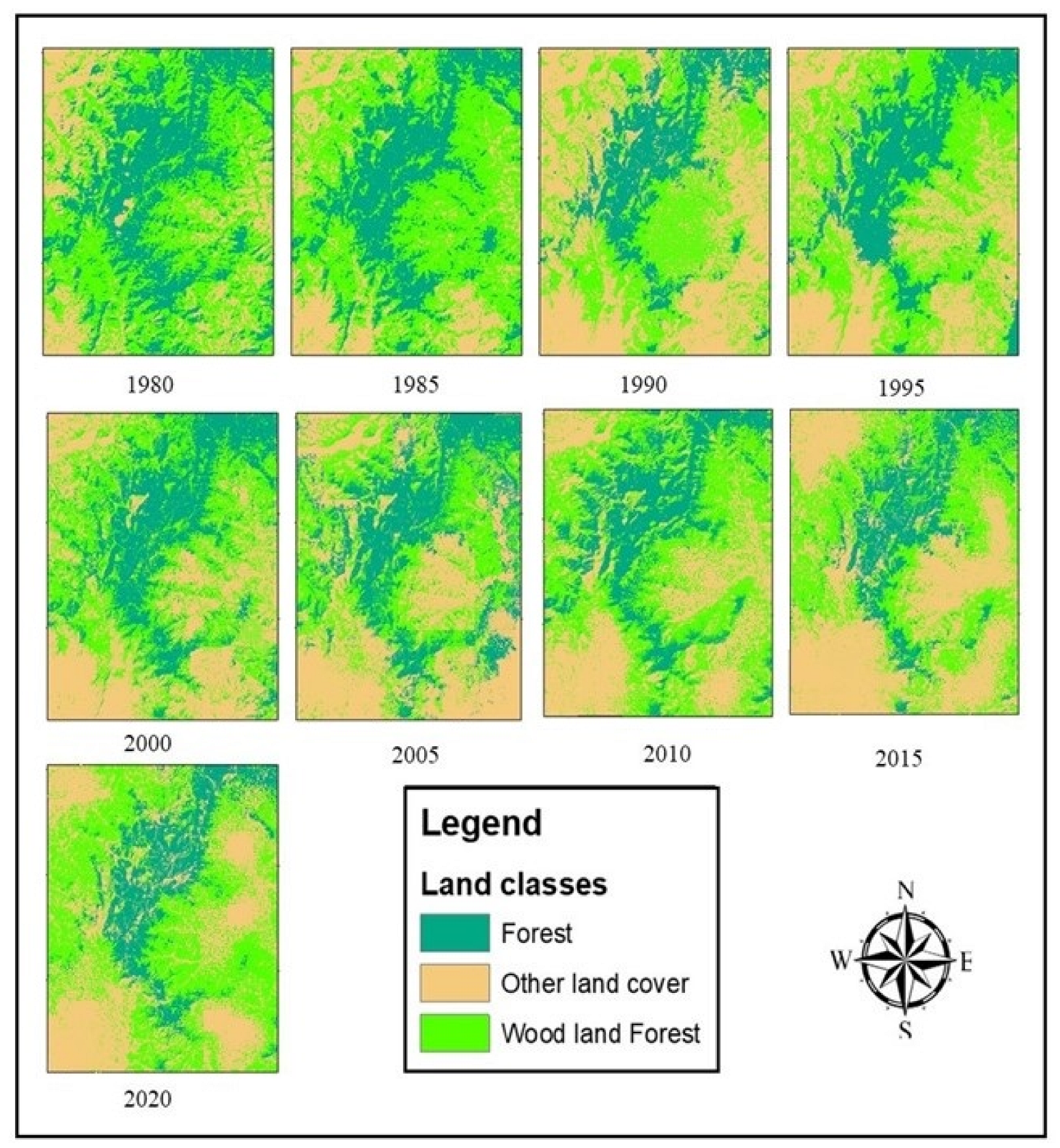
3.1. Land Cover Classification Analysis
3.2. Classification Accuracy Assessment
4. Discussion
Limitations of the Study
5. Conclusions
Author Contributions
Funding
Institutional Review Board Statement
Informed Consent Statement
Data Availability Statement
Conflicts of Interest
References
- Mahmoud, S.H.; Gan, T.Y. Impact of anthropogenic climate change and human activities on environment and ecosystem services in arid regions. Sci. Total Environ. 2018, 633, 1329–1344. [Google Scholar] [CrossRef] [PubMed]
- Bonan, G.B. Forests and climate change: Forcings, feedbacks, and the climate benefits of forests. Science 2008, 320, 1444–1449. [Google Scholar] [CrossRef] [PubMed]
- Gebrehiwot, S.G.; Bewket, W.; Gärdenäs, A.I.; Bishop, K. Forest cover change over four decades in the Blue Nile Basin, Ethiopia: Comparison of three watersheds. Reg. Environ. Chang. 2014, 14, 253–266. [Google Scholar] [CrossRef]
- Qamer, F.M.; Abbas, S.; Saleem, R.; Shehzad, K.; Ali, H.; Gilani, H. Forest Cover Change Assessment in Conflict-Affected Areas of Northwest Pakistan: The Case of Swat and Shangla Districts. J. Mt. Sci. 2012, 9, 297–306. [Google Scholar] [CrossRef]
- Marland, G.; Pielke, R.A., Sr.; Apps, M.; Avissar, R.; Betts, R.A.; Davis, K.J.; Frumhoff, P.C.; Jackson, S.T.; Joyce, L.A.; Kauppi, P.; et al. The climatic impacts of land surface change and carbon management, and the implications for climate-change mitigation policy. Clim. Policy 2003, 3, 149–157. [Google Scholar] [CrossRef]
- Keenan, R.J.; Reams, G.A.; Achard, F.; de Freitas, J.V.; Grainger, A.; Lindquist, E. Dynamics of global forest area: Results from the FAO Global Forest Resources Assessment 2015. For. Ecol. Manag. 2015, 352, 9–20. [Google Scholar] [CrossRef]
- FAO. FRA 2015, Terms and Definitions. Forest Resources Assessment, Working Paper 180. Food and Agriculture Organization of the United Nations. 2012, Volume 36. Available online: www.fao.org/forestry/fra (accessed on 4 October 2022).
- Anon. 352 Forest Ecology and Management Global Forest Resources Assessment 2015. Available online: http://www.fao.org/forestry/fra2005/en/ (accessed on 6 October 2022).
- Morales-Barquero, L.; Skutsch, M.; Jardel-Peláez, E.J.; Ghilardi, A.; Kleinn, C.; Healey, J.R. Operationalizing the Definition of Forest Degradation for REDD+, with Application to Mexico. Forests 2014, 5, 1653–1681. [Google Scholar] [CrossRef]
- MacDicken, K.G. Global Forest Resources Assessment 2015: What, Why and How? For. Ecol. Manag. 2015, 352, 3–8. [Google Scholar] [CrossRef]
- Qamer, F.M.; Shehzad, K.; Abbas, S.; Murthy, M.S.R.; Xi, C.; Gilani, H.; Bajracharya, B. Mapping deforestation and forest degradation patterns in Western Himalaya, Pakistan. Remote Sens. 2016, 8, 385. [Google Scholar] [CrossRef]
- Brink, A.B.; Eva, H.D. Monitoring 25 years of land cover change dynamics in Africa: A sample based remote sensing approach. Appl. Geogr. 2009, 29, 501–512. [Google Scholar] [CrossRef]
- Bouslihim, Y.; Kharrou, M.H.; Miftah, A.; Attou, T.; Bouchaou, L.; Chehbouni, A. Comparing Pan-sharpened Landsat-9 and Sentinel-2 for Land-Use Classification Using Machine Learning Classifiers. J. Geovisualization Spat. Anal. 2022, 6, 35. [Google Scholar] [CrossRef]
- Reddy, C.; Sudhakar, C.; Jha, S.; Dadhwal, V.K. Assessment and Monitoring of Long-Term Forest Cover Changes in Odisha, India Using Remote Sensing and GIS. Environ. Monit. Assess. 2013, 185, 4399–4415. [Google Scholar] [CrossRef] [PubMed]
- Sohail, M.; Ali, S.S.F.; Fatima, E.; Nawaz, D.A. Spatio-temporal analysis of land use dynamics and its potential implications on land surface temperature in lahore district, punjab, pakistan. Int. Arch. Photogramm. Remote Sens. Spatial Inf. Sci. 2021, XLIII-B3-2021, 359–367. [Google Scholar] [CrossRef]
- Otukei, J.R.; Blaschke, T. Land cover change assessment using decision trees, support vector machines and maximum likelihoodclassification algorithms. Int. J. Appl. Earth Obs. Geoinf. 2010, 12, S27–S31. [Google Scholar]
- Alzubaidi, L.; Zhang, J.; Humaidi, A.J.; Al-Dujaili, A.; Duan, Y.; Al-Shamma, O.; Santamaría, J.; Fadhel, M.A.; Al-Amidie, M.; Farhan, L. Review of deep learning: Concepts, CNN architectures, challenges, applications, future directions. J. Big Data 2021, 8, 1–74. [Google Scholar]
- Naushad, R.; Kaur, T.; Ghaderpour, E. Deep Transfer Learning for Land Use and Land Cover Classification: A Comparative Study. Sensors 2021, 21, 8083. [Google Scholar] [CrossRef]
- Pires de Lima, R.; Marfurt, K. Convolutional neural network for remote-sensing scene classification: Transfer learning analysis. Remote Sens. 2019, 12, 86. [Google Scholar] [CrossRef]
- Badhe, A.; Chang, S. Fast image classification by boosting fuzzy classifier. Neural Netw. Mach. Learn. 2016, 327, 175–182. [Google Scholar]
- Kamavisdar, P.; Saluja, S.; Agrawal, S. A survey on image classification approaches and techniques. Int. J. Adv. Res. Comput. Commun. Eng. 2013, 2, 1005–1009. [Google Scholar]
- Thanh Noi, P.; Kappas, M. Comparison of Random Forest, k-Nearest Neighbor, and Support Vector Machine Classifiers for LandCover Classification Using Sentinel-2 Imagery. Sensors 2018, 18, 18. [Google Scholar] [CrossRef]
- Tassi, A.; Gigante, D.; Modica, G.; Di Martino, L.; Vizzari, M. Pixel-vs. Object-Based Landsat 8 Data Classification in Google EarthEngine Using Random Forest: The Case Study of Maiella National Park. Remote Sens. 2021, 13, 2299. [Google Scholar] [CrossRef]
- Wang, C.; Shu, Q.; Wang, X.; Guo, B.; Liu, P.; Li, Q. A random forest classifier based on pixel comparison features for urban LiDAR data. ISPRS J. Photogramm. Remote Sens. 2019, 148, 75–86. [Google Scholar] [CrossRef]
- Belgiu, M.; Drăguţ, L. Random forest in remote sensing: A review of applications and future directions. ISPRS J. Photogramm. Remote Sens. 2016, 114, 24–31. [Google Scholar] [CrossRef]
- Chapman, D.S. Random Forest Characterization of Upland Vegetation and Management Burning from Aerial Imagery. J. Biogeogr. 2010, 37, 37–46. [Google Scholar] [CrossRef]
- Sesnie, S.E.; Gessler, P.; Finegan, B.; Thessler, S. Integrating Landsat TM and SRTM-DEM Derived Variables with Decision Trees for Habitat Classification and Change Detection in Complex Neotropical Environments. Remote Sens. Environ. 2008, 112, 2145–2159. [Google Scholar] [CrossRef]
- Van Beijma, S.; Comber, A.; Lamb, A. Random forest classification of salt marsh vegetation habitats using quad-polarimetric airborne SAR, elevation and optical RS data. Remote Sens. Environ. 2014, 149, 118–129. [Google Scholar] [CrossRef]
- Saeys, Y.; Inza, I.; Larrañaga, P. A review of feature selection techniques in bioinformatics. Bioinformatics 2007, 23, 2507–2517. [Google Scholar] [CrossRef]
- Baumann, M.; Ozdogan, M.; Wolter, P.T.; Krylov, A.; Vladimirova, N.; Radeloff, V.C. Landsat remote sensing of forest windfall disturbance. Remote Sens. Environ. 2014, 143, 171–179. [Google Scholar] [CrossRef]
- Chasmer, L.; Hopkinson, C.; Veness, T.; Quinton, W.; Baltzer, J. A decision-tree classification for low-lying complex land cover types within the zone of discontinuous permafrost. Remote Sens. Environ. 2014, 143, 73–84. [Google Scholar] [CrossRef]
- Dronova, I.; Gong, P.; Wang, L.; Zhong, L. Mapping dynamic cover types in a large seasonally flooded wetland using extended principal component analysis and object-based classification. Remote Sens. Environ. 2015, 158, 193–206. [Google Scholar] [CrossRef]
- Sohail, M.; Ali, S.S.F. Abidullah: Monitoring Vegetation Density Using Spectral Vegetation Indices: A Case Study of Malam Jabba Region, District Swat, Pakistan. Int. Arch. Photogramm. Remote Sens. Spatial Inf. Sci. 2022, XLVI-M-2-2022, 185–190. [Google Scholar] [CrossRef]
- Silleos, N.G.; Alexandridis, T.K.; Gitas, I.Z.; Perakis, K. Vegetation Indices: Advances Made in Biomass Estimation and Vegetation Monitoring in the Last 30 Years. Geocarto Int. 2006, 21, 21–28. [Google Scholar] [CrossRef]
- Diaz-Uriarte, R.; Alvarez de Andres, S. Gene selection and classification of microarray data using random forest. BMC Bioinform. 2006, 7, 3. [Google Scholar] [CrossRef] [PubMed]
- Lund, H. Gyde. Definitions of Forest, Deforestation, Afforestation, and Reforestation. Gainesville, VA: Forest Information Services. Misc. pagination. 2015, Volume 14. Available online: https://www.researchgate.net/publication/259821294_Definitions_of_Forest_Deforestation_Afforestation_and_Reforestation (accessed on 2 October 2022).
- Butt, A.; Shabbir, R.; Ahmad, S.S.; Aziz, N. Land use change mapping and analysis using Remote Sensing and GIS: A case study of Simly watershed, Islamabad, Pakistan. Egypt. J. Remote. Sens. Space Sci. 2015, 18, 251–259. [Google Scholar] [CrossRef]
- Iqbal, M.F.; Khan, I.A. Spatiotemporal land use land coverchange analysis and erosion risk mapping of Azad Jammu and Kashmir, Pakistan. Egypt. J. Remote Sens. Space Sci. 2014, 17, 209–229. [Google Scholar]
- Bwangoy, J.R.; Hansen, M.C.; Roy, D.P.; De Grandi, G.; Justice, C.O. Wetland mapping in the Congo Basin using optical and radar remotely sensed data and derived topographical indices. Remote Sens. Environ. 2010, 114, 73–86. [Google Scholar] [CrossRef]
- Petta, R.A.; Carvalho, L.V.; Erasmi, S.; Jones, C. Evaluation of desertification processes in serido region (NE Brazil). Int. J. Geosci. 2013, 4, 12–17. [Google Scholar] [CrossRef]
- Karathanassi, V.; Kolokousis, P.; Ioannidou, S. A comparison study on fusion methods using evaluation indicators. Int. J. Remote Sens. 2007, 28, 2309–2341. [Google Scholar] [CrossRef]
- Khelifi, L.; Mignotte, M. Deep Learning for Change Detection in Remote Sensing Images: Comprehensive Review and Meta-Analysis. IEEE Access 2020, 8, 126385–126400. [Google Scholar] [CrossRef]
- Bhatti, S.S.; Tripathi, N.K. Built-up area extraction using Landsat 8 OLI imagery. GIScience Remote Sens. 2014, 51, 445–467. [Google Scholar] [CrossRef]
- Jeevalakshmi, D.; Reddy, S.N.; Manikiam, B. Land cover classification based on NDVI using LANDSAT8 time series: A case study Tirupati region. In Proceedings of the 2016 International Conference on Communication and Signal Processing (ICCSP), Melmaruvathur, India, 6–8 April 2016; pp. 1332–1335. [Google Scholar]
- Liu, H.Q.; Huete, A. A feedback-based modification of the NDVI to minimize canopy background and atmospheric noise. IEEE Trans. Geosci. Remote Sens. 1995, 33, 457–465. [Google Scholar] [CrossRef]
- Li, P.; Jiang, L.; Feng, Z. Cross-comparison of vegetationindices derived from Landsat-7 Enhanced Thematic Mapper Plus(ETM+) and Landsat-8 operational land imager (OLI) Sensors. Remote Sens. 2014, 6, 310–329. [Google Scholar] [CrossRef]
- Zhang, X.; Delu, P.; Chen, J.; Zhan, Y.; Mao, Z. Using longtime series of Landsat data to monitor impervious surface dynamics a case study in the Zhoushan Islands. J. Appl. Remote Sens. 2013, 7, 073515. [Google Scholar] [CrossRef]
- Huete, A.; Didan, K.; Miura, T.; Rodriguez, E.; Gao, X.; Ferreira, L. Overview of the radiometric and biophysical performance of the MODIS vegetation indices. Remote Sens. Environ. 2002, 83, 195–213. [Google Scholar] [CrossRef]
- Rasul, A.; Balzter, H.; Ibrahim, G.R.F.; Hameed, H.M.; Wheeler, J.; Adamu, B.; Ibrahim, S.; Najmaddin, P.M. Applying Built-Up and Bare-Soil Indices from Landsat 8 to Cities in Dry Climates. Land 2018, 7, 81. [Google Scholar] [CrossRef]
- Madanian, M.; Soffianian, A.R.; Koupai, S.S.; Pourmanafi, S.; Momeni, M. Analyzing the effects of urban expansion on land surface temperature patterns by landscape metrics: A case study of Isfahan city, Iran. Environ. Monit. Assess. 2018, 190, 189. [Google Scholar] [CrossRef]
- Kaimaris, D.; Patias, P. Identification and Area Measurement of the Built-up Area with the Built-up Index (BUI). Int. J. Adv. Remote Sens. GIS 2016, 5, 1844–1858. [Google Scholar] [CrossRef]
- Abdi, A.M. Land cover and land use classification performance of machine learning algorithms in a boreal landscape using Sentinel-2 data. GIScience Remote. Sens. 2020, 57, 1–20. [Google Scholar] [CrossRef]
- Paul, D.; Su, R.; Romain, M.; Sébastien, V.; Pierre, V.; Isabelle, G. Feature selection for outcome prediction in oesophageal cancerusing genetic algorithm and random forest classifier. Comput. Med. Imaging Graph. 2017, 60, 42–49. [Google Scholar] [CrossRef]
- Storey, E.A.; Stow, D.A.; O’Leary, J.F. Assessing postfire recovery of chamise chaparral using multi-temporal spectral vegetationindex trajectories derived from Landsat imagery. Remote Sens. Environ. 2016, 183, 53–64. [Google Scholar] [CrossRef]
- Talukdar, S.; Singha, P.; Mahato, S.; Pal, S.; Liou, Y.-A.; Rahman, A. Land-use land-cover classification by machine learning classifiers for satellite observations—A review. Remote Sens. 2020, 12, 1135. [Google Scholar] [CrossRef]
- Domenikiotis, C.; Spiliotopoulos, M.; Tsiros, E.; Dalezios, N.R. Early Cotton Yield Assessment by the Used of the NOAA/AVHRR Derived Vegetation Condition Index (VCI) in Greece. Int. J. Remote Sens. 2004, 25, 2807–2819. [Google Scholar] [CrossRef]
- Naqvi, H.R.; Siddiqui, L.; Devi, L.M.; Siddiqui, M.A. Landscape transformation analysis employing compound interest formula in the Nun Nadi Watershed, India. Egypt. J. Remote Sens. Space Sci. 2014, 17, 149–157. [Google Scholar]
- Jensen, J.R. Introductory Digital Image Processing: A Remote Sensing Perspective; Prentice-Hall Inc.: Hoboken, NJ, USA, 1996. [Google Scholar]
- Xiang, M.; Hung, C.-C.; Pham, M.; Kuo, B.-C.; Coleman, T. A parallelepiped multispectral image classifier using genetic algorithms. In Proceedings of the 2005 IEEE International Geoscience and Remote Sensing Symposium, IGARSS ‘05, Seoul, Korea, 29 July 2005; Volume 1, p. 4. [Google Scholar]
- Olofsson, P.; Foody, G.M.; Stehman, S.V.; Woodcock, C.E. Making better use of accuracy data in land change studies: Estimatingaccuracy and area and quantifying uncertainty using stratified estimation. Remote Sens. Environ. 2013, 129, 122–131. [Google Scholar] [CrossRef]
- Wulder, M.A.; White, J.C.; Goward, S.N.; Masek, J.G.; Irons, J.R.; Herold, M.; Cohen, W.B.; Loveland, T.R.; Woodcock, C.E. Landsatcontinuity: Issues and opportunities for land cover monitoring. Remote Sens. Environ. 2008, 112, 955–969. [Google Scholar] [CrossRef]
- Soni, P.K.; Rajpal, N.; Mehta, R.; Mishra, V.K. Urban land cover and land use classification using multispectral sentinal-2 imagery. Multimedia Tools Appl. 2021, 81, 36853–36867. [Google Scholar] [CrossRef]
- Tateishi, R. Remote Sensing and GIS for Mapping and Monitoring Land Cover and Land-Used Changes in the Northwestern Coastal Zone of Egypt. Appl. Geogr. 2007, 27, 28–41. [Google Scholar]
- Chaaban, F.; El Khattabi, J.; Darwishe, H. Accuracy Assessment of ESA WorldCover 2020 and ESRI 2020 Land Cover Maps for a Region in Syria. J. Geovisualization Spat. Anal. 2022, 6, 31. [Google Scholar] [CrossRef]
- Churches, C.E.; Wampler, P.J.; Sun, W.; Smith, A.J. Evaluation of forest cover estimates for Haiti using supervised classification of Landsat data. Int. J. Appl. Earth Obs. Geoinf. 2014, 30, 203–216. [Google Scholar] [CrossRef]
- Ghebrezgabher, M.G.; Yang, T.; Yang, X.; Wang, X.; Khan, M. Extracting and Analyzing Forest and Woodland Cover Change in Eritrea Based on Landsat Data Using Supervised Classification. Egypt. J. Remote Sens. Space Sci. 2016, 19, 37–47. [Google Scholar] [CrossRef]
- Liu, C.; Frazier, P.; Kumar, L. Comparative assessment of the measures of thematic classification accuracy. Remote Sens. Environ. 2007, 107, 606–616. [Google Scholar] [CrossRef]
- Nyberg, G.; Knutsson, P.; Ostwald, M.; Öborn, I.; Wredle, E.; Otieno, D.J.; Mureithi, S.; Mwangi, P.; Said, M.Y.; Jirström, M.; et al. Enclosures in West Pokot, Kenya: Transforming land, livestock and livelihoods in drylands. Pastoralism 2015, 5, 25. [Google Scholar] [CrossRef]
- Wibowo, A.; Ismullah, I.H.; Dipokusumo, B.S.; Wikantika, K. Land Degradation Model Based on Vegetation and Erosion Aspects Using Remote Sensing Data. ITB J. Sci. 2012, 44, 19–34. [Google Scholar] [CrossRef]
- Yang, X.; Xu, B.; Jin, Y.; Qin, Z.; Ma, H.; Li, J.; Zhao, F.; Chen, S.; Zhu, X. Remote sensing monitoring of grassland vegetation growth in the Beijing–Tianjin sandstorm source project area from 2000 to 2010. Ecol. Indic. 2014, 51, 244–251. [Google Scholar] [CrossRef]
- Rwanga, S.S.; Ndambuki, J.M. Accuracy Assessment of Land Used/Land Cover Classification Using Remote Sensing and GIS. Int. J. Geosci. 2017, 8, 611–622. Available online: http://www.scirp.org/journal/doi.aspx?DOI=10.4236/ijg.2017.84033 (accessed on 2 October 2022). [CrossRef]
- Huete, A.R. A soil-adjusted vegetation index (SAVI). Remote Sens. Environ. 1988, 25, 295–309. [Google Scholar] [CrossRef]
- FAO. Country Report Eritrea, Global Forest ResourcesAssessment (FRA); FRA2010/063; Food and Agriculture Organization of theUnited Nations: Rome, Italy, 2010. [Google Scholar]
- Gitelson, A.A.; Kaufman, Y.J.; Merzlyak, M.N. Use of a green channel in remote sensing of global vegetation from EOS-MODIS. Remote Sens. Environ. 1996, 58, 289–298. [Google Scholar] [CrossRef]
- Ehlers, M. Remote Sensing and Geographic Information Systems: Image-Integrated Geographic Information Systems. Geogr. Inf. Syst. (GIS) Mapp. -Pract. Stand. 1992, 53–67. [Google Scholar] [CrossRef]
- Shehzad, K.; Qamer, F.M.; Murthy, M.S.R.; Abbas, S.; Bhatta, L.D. Deforestation Trends and Spatial Modelling of Its Drivers in the Dry Temperate Forests of Northern Pakistan—A Case Study of Chitral. J. Mt. Sci. 2014, 11, 1192–1207. [Google Scholar] [CrossRef]
- Sfm-project, K. Base Line Studies of the Shahran (Manchi) Forest, Kaghan (Sfm-Project)-2017. Available online: https://info.undp.org/docs/pdc/Documents/PAK/Kaghan%20Report-%20(SFM)%20Jan-2018%20(Final)%20Gilani.pdf (accessed on 4 October 2022).
- FAO. Natural forest formation, Eritrea, forest cover map. Forest Resources Assessment (FRA). Food Agric. Organ. United Nations 2000, 352, 9–14. [Google Scholar] [CrossRef]
- López, S.; Sierra, R. Agricultural change in the Pastaza River Basin: A spatially explicit model of native Amazonian cultivation. Appl. Geogr. 2010, 30, 355–369. [Google Scholar] [CrossRef]
- Bratley, K.; Ghoneim, E. Modeling urban encroachment on the agricultural land of the eastern Nile Delta using remote sensing and a GIS-based Markov chain model. Land 2018, 7, 114. [Google Scholar] [CrossRef]
- Marconcini, M.; Keil, M. Combined use of multi-seasonal high and medium resolution satellite imagery for parcel-related mapping of cropland and grassland. Int. J. Appl. Earth Obs. Geoinf. 2014, 28, 230–237. [Google Scholar] [CrossRef]
- Tigges, J.; Lakes, T.; Hostert, P. Urban vegetation classification: Benefits of multitemporal RapidEye satellite data. Remote Sens. Environ. 2013, 136, 66–75. [Google Scholar] [CrossRef]
- Karlson, M. Remote Sensing of Woodland Structure and Composition in the Sudano-Sahelian zone: Application of WorldView-2 and Landsat 8; Linköping University: Linköping, Sweden, 2015. [Google Scholar]
- Bredemeier, M.; Dohrenbusch, A. Afforestation and Reforestation. Biodivers. Struct. Funct. -Vol. II 2009, 2, 219. [Google Scholar] [CrossRef]
- Gandhi, G.M.; Parthiban, S.; Thummalu, N.; Christy, A. Ndvi: Vegetation Change Detection Using Remote Sensing and Gis—A Case Study of Vellore District. Procedia Comput. Sci. 2015, 57, 1199–1210. [Google Scholar] [CrossRef]
- Ahmed, Z.; Asghar, M.M.; Malik, M.N.; Nawaz, K. Moving towards a sustainable environment: The dynamic linkage between natural resources, human capital, urbanization, economic growth, and ecological footprint in China. Resour. Policy 2020, 67, 101677. [Google Scholar] [CrossRef]
- Du, L.; Tian, Q.; Yu, T.; Meng, Q.; Jancso, T.; Udvardy, P.; Huang, Y. A Comprehensive Drought Monitoring Method Integrating MODIS and TRMM Data. Int. J. Appl. Earth Obs. Geoinf. 2013, 23, 245–253. [Google Scholar] [CrossRef]
- Fischer, K.M.; Khan, M.H.; Gandapur, A.K.; Rao, A.L.; Zarif, R.M.; Marwat, H. Study on Timber Harvesting Ban in NWFP, Pakistan; Intercooperation Head Office: Berne, Switzerland, 2010. [Google Scholar]
- Act, Forest Conservation. Definition of Forests—A Review Introduction: (Phase Iv): 1980, 1–15. Available online: https://mpforest.gov.in/img/files/Handbook_FC_Act_2019.pdf (accessed on 1 October 2022).
- Shah, S.W.A. Political Reforms in the Federally Administered Tribal Areas of Pakistan (FATA): Will It End the Current Militancy? SAI 2012, 64, 1617–5069. [Google Scholar]
- El Baroudy, A.A.; Moghanm, F.S. Combined use of remote sensing and GIS for degradation risk assessment in some soils of the Northern Nile Delta, Egypt. Egypt. J. Remote Sen. Space Sci. 2014, 17, 77–85. [Google Scholar] [CrossRef]


| Satellite Instrument | Spatial Resolution | Temporal Availability |
|---|---|---|
| Landsat MMS | 60 m | 1980 |
| Landsat TM | 30 m | 1985, 1990,1995 |
| Landsat ETM+ | 30 m | 2000, 2010 |
| Landsat OLI | 30 m | 2015, 2020 |
| Digital elevation model (SRTM) | 30 m |
| Land Cover Classes | Training Pixels | Validation Pixels |
|---|---|---|
| Forest cover | 21,434 | 9356 |
| Woodland cover | 32,224 | 13,410 |
| Other land cover | 16,342 | 7234 |
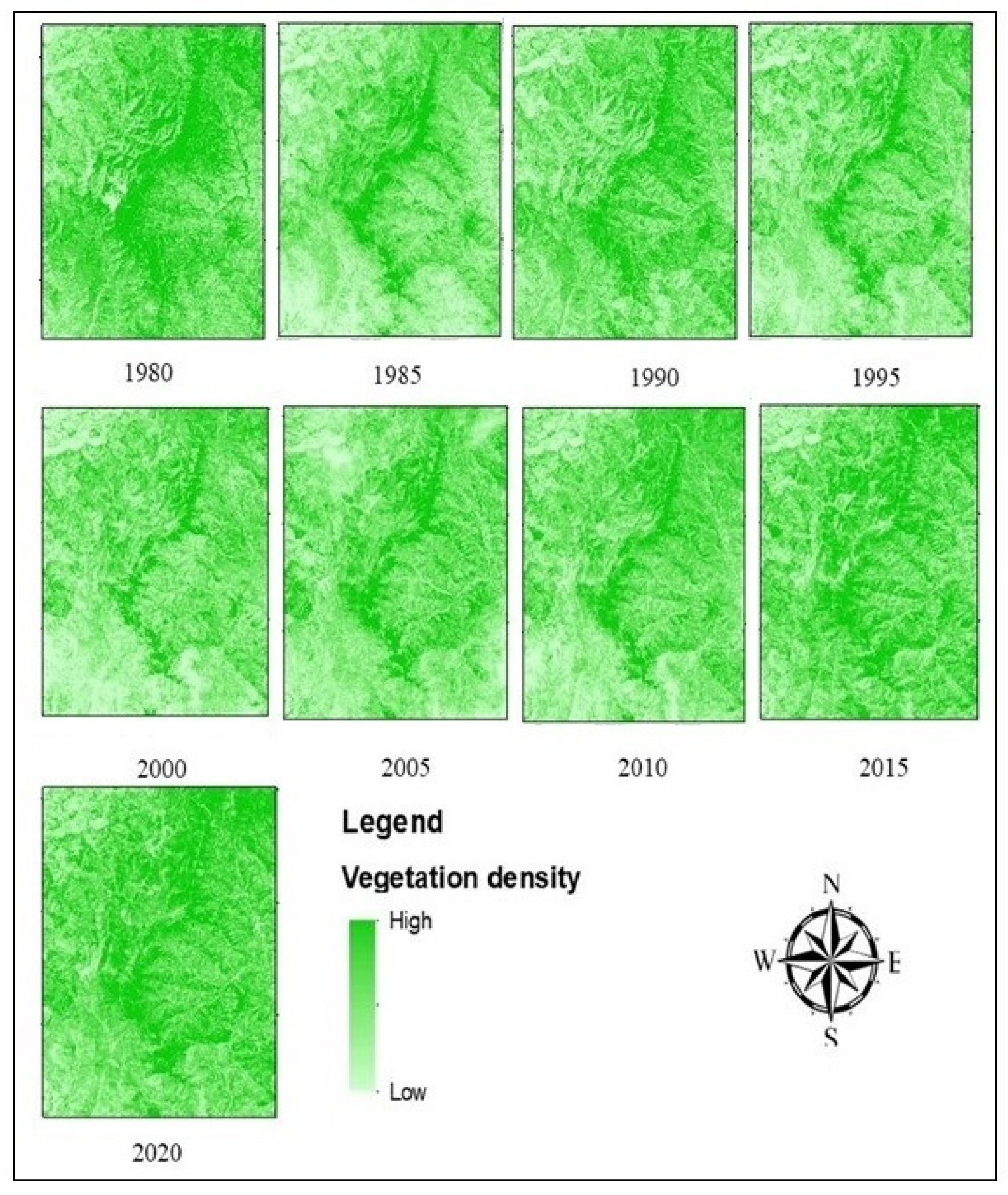
| Vegetation Cover | NDVI | VCP | SAVI | DEM |
|---|---|---|---|---|
| High to very High | >0.45 | >0.75 | >0.45 | >1700 |
| Medium | 0.35–0.55 | 0.55–0.75 | 0.28–0.53 | 1250–1700 |
| Low to very low | <0.25 | <0.55 | <0.33 | 800–1250 |
| Land Classes | 1980 | 1985 | 1990 | 1995 | 2000 | 2005 | 2010 | 2015 | 2020 |
|---|---|---|---|---|---|---|---|---|---|
| Forest | 236 | 227 | 210 | 196 | 183 | 169 | 135 | 141 | 152 |
| Woodland | 381 | 374 | 369 | 306 | 295 | 278 | 263 | 259 | 287 |
| Other land | 178 | 194 | 216 | 293 | 317 | 348 | 384 | 395 | 356 |
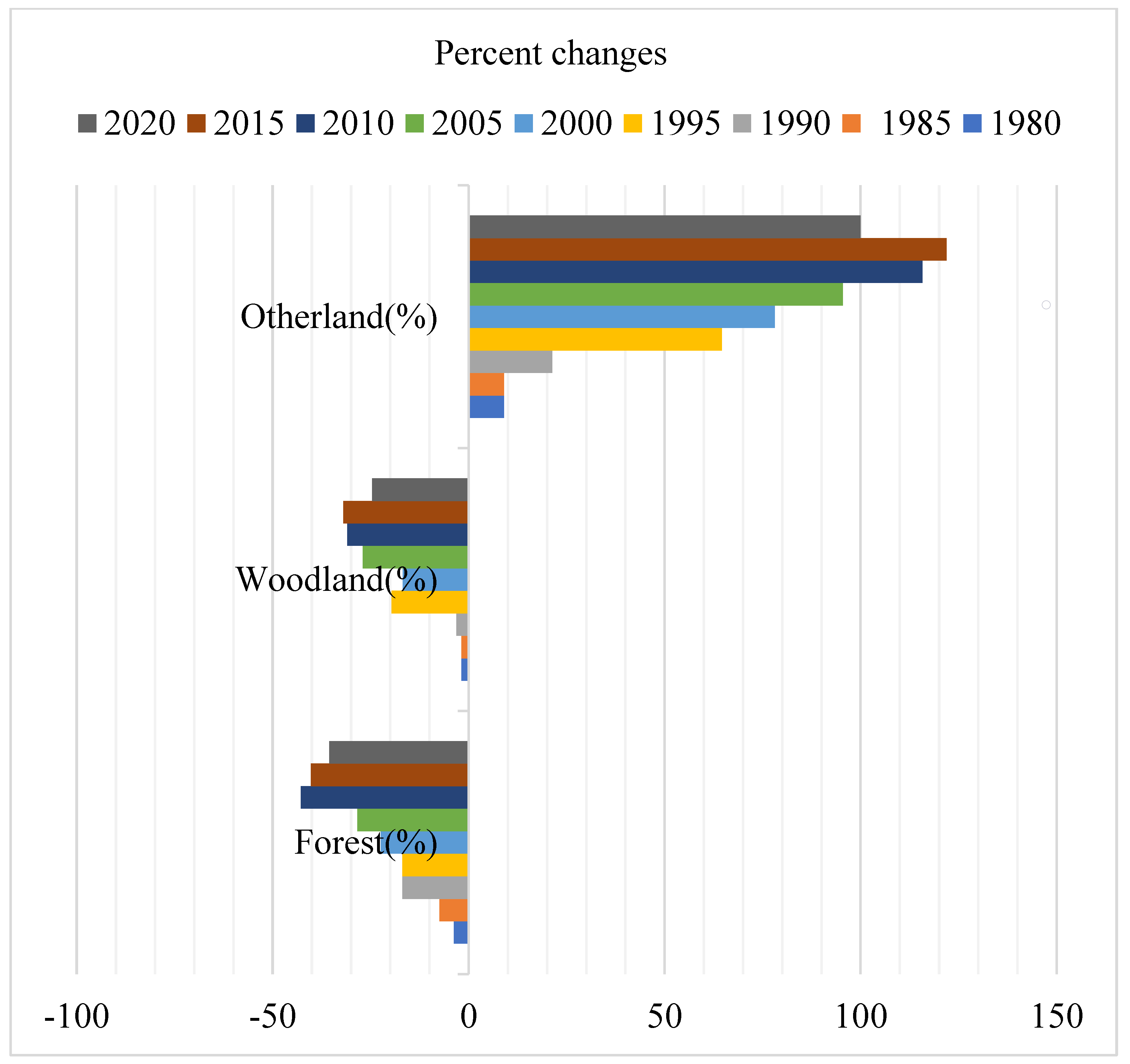
| Change in Land Cover Classes (%) | 1980 | 1985 | 1990 | 1995 | 2000 | 2005 | 2010 | 2015 | 2020 |
|---|---|---|---|---|---|---|---|---|---|
| Forest | 0 | −7 | −16.5 | −16.9 | −22 | −28 | −42 | −40 | −35 |
| Woodland | 0 | −1 | −3 | −19 | −16 | −27 | −30 | −32 | −24 |
| Other land | 0 | 8 | 21 | 64 | 78 | 95 | 115 | 121 | 100 |
| Year | OA | Kappa | Average Accuracy | Average F1-Score | Average Precision | Average Recall |
|---|---|---|---|---|---|---|
| 1980 | 91.58 | 0.9 | 0.89 | 0.87 | 0.86 | 0.89 |
| 1985 | 92.67 | 0.91 | 0.95 | 0.89 | 0.84 | 0.87 |
| 1990 | 93.55 | 0.92 | 0.99 | 0.85 | 0.87 | 0.91 |
| 1995 | 94.68 | 0.93 | 0.99 | 0.86 | 0.84 | 0.85 |
| 2000 | 96.64 | 0.94 | 0.98 | 0.89 | 0.94 | 0.96 |
| 2005 | 94.18 | 0.91 | 0.99 | 0.84 | 0.91 | 0.94 |
| 2015 | 95.73 | 0.96 | 0.99 | 0.94 | 0.86 | 0.87 |
| 2020 | 94.49 | 0.93 | 0.99 | 0.93 | 0.91 | 0.93 |
Disclaimer/Publisher’s Note: The statements, opinions and data contained in all publications are solely those of the individual author(s) and contributor(s) and not of MDPI and/or the editor(s). MDPI and/or the editor(s) disclaim responsibility for any injury to people or property resulting from any ideas, methods, instructions or products referred to in the content. |
© 2023 by the authors. Licensee MDPI, Basel, Switzerland. This article is an open access article distributed under the terms and conditions of the Creative Commons Attribution (CC BY) license (https://creativecommons.org/licenses/by/4.0/).
Share and Cite
Junaid, M.; Sun, J.; Iqbal, A.; Sohail, M.; Zafar, S.; Khan, A. Mapping LULC Dynamics and Its Potential Implication on Forest Cover in Malam Jabba Region with Landsat Time Series Imagery and Random Forest Classification. Sustainability 2023, 15, 1858. https://doi.org/10.3390/su15031858
Junaid M, Sun J, Iqbal A, Sohail M, Zafar S, Khan A. Mapping LULC Dynamics and Its Potential Implication on Forest Cover in Malam Jabba Region with Landsat Time Series Imagery and Random Forest Classification. Sustainability. 2023; 15(3):1858. https://doi.org/10.3390/su15031858
Chicago/Turabian StyleJunaid, Muhammad, Jianguo Sun, Amir Iqbal, Mohammad Sohail, Shahzad Zafar, and Azhar Khan. 2023. "Mapping LULC Dynamics and Its Potential Implication on Forest Cover in Malam Jabba Region with Landsat Time Series Imagery and Random Forest Classification" Sustainability 15, no. 3: 1858. https://doi.org/10.3390/su15031858
APA StyleJunaid, M., Sun, J., Iqbal, A., Sohail, M., Zafar, S., & Khan, A. (2023). Mapping LULC Dynamics and Its Potential Implication on Forest Cover in Malam Jabba Region with Landsat Time Series Imagery and Random Forest Classification. Sustainability, 15(3), 1858. https://doi.org/10.3390/su15031858