An Optimum User Association Algorithm in Heterogeneous 5G Networks Using Standard Deviation of the Load

Abstract

Fifth-generation (5G) wireless networks and beyond will be heterogeneous in nature, with a mixture of macro and micro radio cells. In this scenario where high power macro base stations (MBS) coexist with low power micro base stations (mBS), it is challenging to ensure optimal usage of radio resources to serve users with a multitude of quality of service (QoS) requirements. Typical signal to interference and noise ratio (SINR)-based user allocation protocols unfairly assign more users to the high power MBS, starving mBS. There have been many attempts in the literature to forcefully assign users to mBS with limited success. In this paper, we take a different approach using second order statistics of user data, which is a better indicator of traffic fluctuations. We propose a new algorithm for user association to the appropriate base station (BS) by utilizing the standard deviation of the overall network load. This is done through an exhaustive search of the best user equipment (UE)–BS combinations that provide a global minimum to the standard deviation. This would correspond to the optimum number of UEs assigned to every BS, either macro or micro. We have also derived new expressions for coverage probability and network energy efficiency for analytical performance evaluation. Simulation results prove the validity of our proposed methods to balance the network load, improve data rate, average energy efficiency, and coverage probability with superior performance compared with other algorithms.

1. Introduction

1.1. Background

A key aspect of the emerging fifth-generation and beyond (5G+) wireless networks is the support to multitude of tiers resulting in a Heterogeneous network (HetNet) architecture. This HetNet architecture with the popular network slicing capability shall not only support diverse requirements such as highly varying throughput(s), bit rates, latency, quality of service (QoS) and reliability [1], but also shall have significantly better overall sum-throughput gain, higher energy efficiency, and better coverage [2,3]. Most of these advantages are attributed to having a combination of different size radio cells, from Macro to Micro and even Pico.

However, seamless integration of large and small cells imposes a number of challenges, since different base stations (BSs) will have different transmission powers, coverage areas and data rate capabilities and need to cater different types of user equipment (UE). Therefore, developing a proper UE–BS association algorithm for diverse 5G+ HetNets is a tough task. Such an appropriate algorithm shall not only confirm the QoS performance for each UE, but shall also ensure fairness for both UEs and BSs.

Typical maximum signal to interference and noise ratio (Max-SINR)-based UE association algorithms do not provide a fair load distribution as most of the UEs will be allocated to high power Macro BSs (MBSs), starving low power Micro BSs (mBSs) and undermining the benefits of having multiple tiers in the first place.

In this paper, we propose a novel approach by considering the load distribution across the $whole$ network and by optimizing its variability indicator, in other words, the $standard$ $deviation$ of the network load, which results in fairness to all BSs, both Macro and Micro. The optimum standard deviation reflects the optimum number of UEs associated with every BS. Besides balancing the overall network load, our algorithm also ensures an acceptable level of SINR for all UEs and allocates required bandwidth for each UE without exceeding the available bandwidth from the given Macro/Micro BS. As a result, a UE that is re-associated to another BS will still receive adequate signal strength ensuring adequate quality of service. These are all done in a noticeably short time, suitable to track mobile UEs. In conventional UE association algorithms, either SINR level or load per BS are considered for decision making. However, in our proposed algorithm both SINR level and network load are taken into consideration.

To the best of our knowledge, no other work considering minimizing network load standard deviation as a means of balancing load in HetNets has been reported so far.

This paper is organized as follows. We discuss the HetNet system model in Section 2. We present the derivations for coverage probability and energy efficiency in Section 3. In Section 4 we explain the proposed algorithm. We present the performance analysis in Section 5. Finally, we conclude in Section 6.

1.2. Overview of UE Association Algorithms

Most UE association algorithms either tend to allocate UEs to MBSs that have the strongest transmitted signal power or tend to artificially associate UEs to mBSs. An imbalanced load and resource distribution will arise in the network with these approaches that could severely impair some links. UE association algorithms can be categorized into several types. They can either be based on signal power, biasing, partitioning, selfishness, breathing, optimization, and game theory. In the following lines, we present an overview of various types of UE association algorithms.

Max-SINR [4] has long been used for UE association. However, it tends to connect most UEs to the more powerful MBSs. Besides, it suffers from high computational complexity and it is difficult to compute the SINR and implement the association in real time.

1.2.1. Bias Based User Association

Several authors introduced bias-based algorithms. For example, the cell range expansion algorithm (CRE) is discussed in [5,6], where the signal strength of mBS is artificially enhanced by multiplying it by a certain bias. Here, the performance is variable and depends on the value of the bias. Note, a complex algorithm is needed to decide the optimal bias factor value. This algorithm showed an increase in system throughput and capacity, however the mBSs performance was degraded by strong interference from MBSs (inter-cell interference—ICI) to the offloaded users.

A number of further research efforts [7,8,9,10] focused on optimizing the value of the bias under various constraints. Namely:

• The bias to optimized to maximize the weighted sum energy efficiency in [11],
• The bias to optimized to maximize the sum rate in [12],
• The bias is optimized considering per-user utility function in [8,13],
• The bias is optimized to maximize mean utility per UE, and UE satisfaction in [14].

However, in general, it is a hard task to decide the optimal bias factor value. Furthermore, when the bias is optimized considering a certain factor, some other factors usually suffer.

1.2.2. Inter Cell Interference Based User Association

Some algorithms improved the performance of CRE by applying an ICI mitigation aspect into it. In [15], the authors suggested a reverse frequency allocation (RFA) scheme along with cell range expansion-based user association to combat ICI to mBS UE from the MBS. Also, a selective BS deployment is applied where mBSs are selected in regions where MBS coverage is considerably poor. Likewise, mBSs are muted where the MBS coverage is acceptable to the users.

The authors in [16] proposed another cell association algorithm to mitigate ICI that selectively mutes mBSs. This is how it is done: The available space is divided into inner and outer subspaces. In the inner subspace, end users are associated only with MBS based on received signal power scheme (mBSs are deactivated in this region). In the outer subspace, where MBS coverage is poor, users are associated with either a MBS or a mBS based on a biased or unbiased maximum received power scheme.

1.2.3. Partitioning User Association

The authors of [17] introduced two UE association algorithms, namely time and frequency partitioning offloading algorithms to maximize the users’ long-term sum of utilities rates. The first algorithm performs association using a utility maximization (MAUM) approach, while the other one performs association using an optimized partition and utility (AOPU) approach. Similar to the CRE algorithm, the UEs that are offloaded here from the MBS to mBS might also still receive a strong interference from MBS. To mitigate this across-the-tier interference, MAUM considers a time partitioning method where the serving time is cut into two parts. The MBSs’ can only transmit during the first part, while the mBSs can use both of them. Therefore, some UEs can select the second time portion of the mBS to avoid the strong interference from the MBS. In AOPU, frequency partitioning is also considered to degrade the cross-plane interference. In addition, the time partitioning factor is optimized.

1.2.4. Greedy Algorithms

Few other approaches [18,19,20,21] assume UEs are selfish and try to capture the maximum available bandwidth without consideration for other UEs. These greedy UEs select the BS with the least load to grab all the remaining bandwidth for themselves. This selfish approach causes bandwidth imbalance in the network and failure in some links. Also, the aforementioned approach does not consider the overall network balance.

Also in [22], the authors considered two association algorithms; one is a greedy linear programming heuristic where UEs are associated to BSs that have enough capacity and are not overloaded. The other algorithm is a distributed probabilistic strategy that gives privilege to the BSs with greater availability (percentage of available capacity) and less load.

1.2.5. Cell Breathing User Association

In [23], the authors suggested an algorithm to control the BSs’ coverage range using cell breathing. They developed a set of polynomial-time algorithms that find the optimal beacon power settings which minimize the load of the most congested BS. Some work was introduced in the literature based on traffic transfer from heavily loaded to lightly loaded BSs in an effort to balance the load. Also using the cell breathing technique for WLAN networks, the authors in [24] optimized system throughput with constraints on UEs fairness and load balance by associating the UE to the strongest WiFi access point.

1.2.6. Game Theory User Association

Some authors considered game theory to solve user association problems in HetNets [25,26,27]. For example, the authors in [27] proposed a multi-leader multi-follower Stackelberg game architecture to formulate the interaction between BSs and UEs. Each UE chooses the BS that maximizes its payoff (or minimizes its payment) in the follower-level game.

1.2.7. Other User Association Algorithms

In [28], the authors suggested the mobile-assisted connection-admission (MACA) algorithm to connect UEs to less loaded neighboring BSs via some special two-hop links. Also, the authors in [29] suggest a multi-hop connection link and define its network architecture.

Interestingly, the authors of [30,31,32] studied the performance of integrated cellular and ad-hoc relay (ICAR) systems by employing overlay networks (ad hoc networks) on top of the existing cellular networks. Channels are shared between congested and less congested cells via primary and secondary relaying. The issue with these systems are the insufficient number of ad hoc relay channels due to other users’ interference impacting system performance.

In [33], the authors suggested to offload UEs to mBSs that only have a sufficient remaining backhaul capacity. They used specific QoS constraints to maximize the network throughput while the minimum bit rate to a specific UE is met.

The authors of [24] proposed a load-balancing scheme for an operator-deployed cellular-WLAN HetNet to optimize system throughput. The authors in [8] proposed a distributed belief propagation (BP) algorithm to optimize the weighted proportional fairness with various UE priorities. Also, the authors in [34] designed two offloading algorithms to maximize the weighted sum of long-term rates.

Every load balancing algorithm is not optimal and comes with some disadvantages. Biasing algorithms improve load balancing and increase system throughput. However, the performance varies based on the value of the bias which has an impact on other performance metrics. Using partitioning algorithms or cell breathing algorithms may be useful, but the optimal partitioning or coverage range factors are a challenge and performance may even be reduced by an inappropriate choice. Greedy algorithms affect bandwidth imbalance of the whole network.

We compared the performance of our proposed algorithm with those in [4,5,6,17]. Our algorithm helped in balancing the network load, improved data rate, energy efficiency, and coverage.

2. Two-Tier HetNet System Model

Figure 1 shows a multi-tier dense HetNet system, where there are $k;k\in \{1,2,3,\dots ,K\}$ tiers of BSs.

For simplicity, we consider one Macro BS at the center with $N_A$ antennas. There are $N_m$ short-range Micro BSs each with $N_a$ antennas. Locations of the mBSs are obtained by running a homogeneous Poisson point process (PPP) ${\varphi }_k$ of density ${\lambda }_k$. PPP is the best process to model the randomness of locations of BSs [35,36]. The BS transmission power at the $k^{th}$ tier is $P_{T_k}$ and the minimum allowed distance between any two mBSs is $d_{min}$.

Each BS (either Macro or Micro) is serving $u;u\in \{1,2,3,\dots ,U\}$ single-antenna users. Each user has the same transmit power $P_u$ and the user density is ${\lambda }_u$.

The system is assumed to be of open access, which means that there is no restriction on the association of UEs to a certain tier BS. In our model, we consider a block-fading channel model with large and small-scale fading [37]. The large-scale fading is a function of distance and path loss. The same path loss exponent $\alpha$ is considered for both the Macro and Micro tiers. The multi path small-scale fading coefficients are assumed to be Rayleigh distributed.

In this work, we consider two levels of communication; back-haul links between the MBSs and the mBSs, and the access link between the Macro or Micro BS and their associated UEs.

Orthogonal Frequency-Division Multiplexing (OFDM) is considered for the back-haul downlink (from MBS to the associated mBS). Here the MBS schedules transmission over T time-frequency slots.

Orthogonal Frequency and Code Division Multiplexing (OFCDM) is considered for the BS to UE links (access downlinks) as it outperforms OFDM for high speed communications. The system uses coded orthogonal channels where $N_b$ is the number of transmitted bits (each with bit energy $E_b$). Also, N and F are the spreading factors in time and frequency domains respectively. The transmitted signal is spread with Pseudo Noise (PN) sequences in the time domain with chip energy $E_c$ and chip duration $T_c$, where

$$E_c=E_b/(N·F)$$

The total spectrum is divided into groups; each group has Z non-contiguous subcarriers that are equally spaced throughout the spectrum. Groups are denoted by $G_d$, where d = $1,2,3,\dots ,D$. All mBSs use the same sub channels and transmit on the same frequencies.

3. Coverage Probability and Energy Efficiency of the Two-Tier Open Access HetNet

3.1. Coverage Probability Analysis

SINR is a key factor in calculating coverage probability. Downlink SINR from the $k^{th}$ BS to its associated UE u on subcarrier z in an OFCDM channel is:

$$\begin{array}{c}\hfill {\mathit{\gamma }}_{\mathit{k}}^{\left(\mathit{z}\right)}\left({\mathit{d}}_{\mathit{k}}\right)=\frac{N^2{E}_c^2{\lambda }_k{P}_{T_k}{\parallel {\mathbf{d}}_{\mathbf{k}}\parallel }^{-\alpha }{\displaystyle \sum _{z\in G_d}}\left({\mathbf{h}}_{\mathbf{k}}^{\left(z\right)}\right)}{{\displaystyle \sum _{\begin{array}{c}q=1,q\ne k\end{array}}^k}{N}^2{E}_c^2{P}_{T_q}{\parallel {\mathbf{d}}_{\mathbf{q}}\parallel }^{-\alpha }{\displaystyle \sum _{\begin{array}{c}z\in G_d\end{array}}}\left({\mathbf{h}}_{\mathbf{q}}^{\left(z\right)}\right)+{\sigma }_n^2}\end{array}$$

(1)

where $N^2{E}_c^2$ is the signal power considering the PN sequence, $\parallel d_k\parallel$ is the distance from the BS to UE u, ${\mathbf{h}}_{\mathbf{k}}$ is the fading gain from BS k (either Macro or Micro) to u on subcarrier z, ${\sigma }_n^2$ is the noise variance, and $\parallel {\mathbf{d}}_{\mathbf{q}}\parallel$ is the distance from the $q^{th}$ interfering BS; $1\le q\le K$. The interference term ${\mathbf{I}}_{{\mathbf{d}}_{\mathbf{k}}}$ is defined as ${\mathbf{I}}_{{\mathbf{d}}_{\mathbf{k}}}={\displaystyle \sum _{\begin{array}{c}q=1,q\ne k\end{array}}^k}{N}^2{E}_c^2{P}_{T_q}{\parallel {\mathbf{d}}_{\mathbf{q}}\parallel }^{-\alpha }{\displaystyle \sum _{z\in G_d}}\left({\mathbf{h}}_{\mathbf{q}}^{\left(z\right)}\right)$.

Assuming $\mathbb{E}(·)$ as the expected value, the expected data rate per UE for BS k is calculated from the above SINR as:

$$\begin{array}{c}\hfill {\Re }_{\mathbf{k}}^{\left(\mathbf{z}\right)}=\mathbb{E}\left[\frac{W_k}{L_k}{log}_2\left(1+\frac{(N_m-U+1)}{U}{\mathit{\gamma }}_{\mathit{k}}^{\left(\mathit{z}\right)}\right)\right]\end{array}$$

(2)

where $W_k$ is the total bandwidth assigned to each BS, $L_k$ is the BS load, and $\frac{(N_m-U+1)}{U}$ represents the massive multiple input multiple output (MIMO) gain [38,39].

Assuming $L_k$ and ${\gamma }_k$ are independent for tractability [40], we can rewrite (2) as:

$$\begin{array}{c}\hfill {\Re }_{\mathbf{k}}^{\left(\mathbf{z}\right)}=\frac{W_k}{\mathbb{E}\left[L_k\right]}{log}_2\left(1+\frac{(N_m-U+1)}{U}{\mathit{\gamma }}_{\mathit{k}}^{\left(\mathit{z}\right)}\right)\end{array}$$

(3)

where $\mathbb{E}\left[L_k\right]$ is the average number of UEs served by $k^{th}$ tier BS.

Because the UE may or may not be associated with the BS, (3) is re-written as:

$$\begin{array}{c}\hfill {\Re }_{\mathbf{k}}^{\left(\mathbf{z}\right)}={\mathbf{x}}_{\mathbf{k}}\frac{W_k}{\mathbb{E}\left[L_k\right]}{log}_2\left(1+\frac{(N_m-U+1)}{U}{\mathit{\gamma }}_{\mathit{k}}^{\left(\mathit{z}\right)}\right)\end{array}$$

(4)

where ${\mathbf{x}}_{\mathbf{k}}$ is a binary variable denoting whether the UE is associated with the BS or not.

If a typical randomly located UE is in coverage, then it connects to a certain BS whose SINR is above its threshold ${\zeta }_k$. Coverage probability in Cartesian coordinates is shown as:

$$\begin{array}{c}\hfill P_c\left({\gamma }_k\right)=\mathbb{P}\left(\bigcup _{k\in K}\underset{{\mathbf{d}}_{\mathbf{k}}\in {\mathbf{Œ}}_{\mathbf{k}}}{max}{\mathit{\gamma }}_{\mathit{k}}^{\left(\mathit{z}\right)}\left({\mathit{d}}_{\mathit{k}}\right)>{\zeta }_k\right)\end{array}$$

(5)

where $\mathbb{P}(·)$ is the probability of the term in brackets. Assuming that we restrict the UE to connect to only one BS at an instance and from the property that probability of an event can be converted into its expected value (probability can be switched into expectation and vice versa) by taking the expectation of an indicator function that equals one [41], then:

$$\begin{array}{c}\hfill P_c\left({\gamma }_k\right)=\mathbb{E}\left[1\left(\bigcup _{k\in K}\underset{{\mathbf{d}}_{\mathbf{k}}\in {\mathbf{Œ}}_{\mathbf{k}}}{max}{\mathit{\gamma }}_{\mathit{k}}^{\left(\mathit{z}\right)}\left({\mathit{d}}_{\mathit{k}}\right)>{\zeta }_k\right)\right]\end{array}$$

(6)

Following from the union bound:

$$\begin{array}{c}\hfill P_c\left({\gamma }_k\right)=\sum _{k\in K}\mathbb{E}\sum _{{\mathbf{d}}_{\mathbf{k}}\in {\varphi }_k}\left[1({\mathit{\gamma }}_{\mathit{k}}^{\left(\mathit{z}\right)}\left({\mathit{d}}_{\mathit{k}}\right)>{\zeta }_k)\right]\end{array}$$

(7)

$$\begin{array}{c}\hfill P_c\left({\gamma }_k\right)=\sum _{k\in K}{\lambda }_k{N}^2{E}_c^2{\int }_{{\mathbb{R}}^2}\mathbb{P}\left(\frac{P_{T_k}{\mathbf{h}}_{\mathbf{k}}\ell \left({\mathbf{d}}_{\mathbf{k}}\right)}{{\mathbf{I}}_{{\mathbf{d}}_{\mathbf{k}}}+{\sigma }_n^2}>{\zeta }_k\right)\mathrm{d}\left({\mathbf{d}}_{\mathbf{k}}\right)\end{array}$$

(8)

which follows from Campbell Mecke Theorem [42] (states that expectation of a function is summed over a point process to an integral involving the mean measure of the point process), where $\ell \left({\mathbf{d}}_{\mathbf{k},\mathbf{u}}\right)={\parallel {\mathbf{d}}_{\mathbf{k},\mathbf{u}}\parallel }^{-\alpha }$, and $\mathrm{d}(·)$ is the derivative operator.

$$\begin{array}{c}\hfill P_c\left({\gamma }_k\right)=\sum _{k\in K}{\lambda }_k{N}^2{E}_c^2{\int }_{{\mathbb{R}}^2}\mathbb{P}\left(({\mathbf{I}}_{{\mathbf{d}}_{\mathbf{k}}}+{\sigma }_n^2)\le \frac{P_{T_k}{\mathbf{h}}_{\mathbf{k}}\ell \left({\mathbf{d}}_{\mathbf{k}}\right)}{{\zeta }_k}\right)\mathrm{d}\left({\mathbf{d}}_{\mathbf{k}}\right)\end{array}$$

(9)

$$\begin{array}{c}\hfill P_c\left({\gamma }_k\right)=\sum _{k\in K}{\lambda }_k{N}^2{E}_c^2{\int }_{{\mathbb{R}}^2}{\mathcal{L}}_I\left(\frac{{\zeta }_k}{P_{T_k}\ell \left({\mathbf{d}}_{\mathbf{k}}\right)}\right)e^{\frac{-{\zeta }_k{\sigma }_n^2}{P_{T_k}\ell \left({\mathbf{d}}_{\mathbf{k}}\right)}}\mathrm{d}\left({\mathbf{d}}_{\mathbf{k}}\right)\end{array}$$

(10)

which arises from the fact that the channel gains are Rayleigh distributed with unity mean, where ${\mathcal{L}}_I(·)$ represents Laplace transform of interference of the term between the brackets. After simplifications, we prove that the coverage probability is obtained as:

$$\begin{array}{c}\hfill P_c\left({\gamma }_k\right)=\frac{\sqrt{\sigma }}{2}{N}^2{E}_c^2\sum _{k\in K}{\lambda }_k\times {\int }_{{\mathbb{R}}^2}{e}^{\left[\frac{S^2{\sigma }^2}{2}-(\mu +{\sigma }^2)S\right]}\mathrm{d}\left({\mathbf{d}}_{\mathbf{k}}\right)\end{array}$$

(11)

The above equation can be solved analytically.

For a rectangular cell, coverage probability is equal to:

$$\begin{array}{ccc}\hfill P_c\left({\gamma }_k\right)& =& \left(\frac{\sqrt{\sigma }}{2}{N}^2{E}_c^2\right)\sum _{k\in K}{\lambda }_k\times {\int }_{-a}^a{e}^{[\frac{S^2{\sigma }^2}{2}-S(\mu +{\sigma }^2)]}2xy{(x^2+y^2)}^{-1/2}{f}_x\left(x\right)f_y\left(y\right)\mathrm{d}x\mathrm{d}y\hfill \end{array}$$

(12)

where $d\left(d_k\right)=d\left(\sqrt{x^2+y^2}\right)=\frac{1}{2}{(x^2+y^2)}^{-1/2}(2x·2y)\mathrm{d}x\mathrm{d}y,f_x\left(x\right)=\frac{1}{2a},f_y\left(y\right)=\frac{1}{2b}$.

Please see Appendix A for the proof.

3.2. Energy Efficiency Analysis

In this section, we derive a new expression for energy efficiency in multi-tier networks. Let us first define $L_k$ as the number of UEs associated with a tagged BS in $k^{th}$ tier, or in other words, it is the traffic load of a BS in $k^{th}$ tier.

The probability that a tagged UE is connected to a $k^{th}$ tier BS is [43]:

$$\begin{array}{c}\hfill \begin{array}{c}\hfill {\mathbb{P}}_k=\frac{{\lambda }_k{P}_{T_k}^{\frac{2}{\alpha }}}{{\sum }_{k=1}^K{\lambda }_k{P}_{T_k}^{\frac{2}{\alpha }}}\end{array}\end{array}$$

(13)

Definition 1.

If we define $R_{total}$ as the total achievable throughput of the whole network that depends on coverage probability, expected data rate, and BS density, then its equation can be written as:

$$\begin{array}{c}\hfill R_{total}=\sum _{k=1}^K{P}_c\left({\gamma }_k\right){\lambda }_u{\mathbb{P}}_k{\Re }_k\end{array}$$

(14)

Then, the energy efficiency can be calculated as:

$$\begin{array}{c}\hfill {\eta }_{EE}=\frac{R_{total}}{{\sum }_{k=1}^K{\lambda }_k{P}_k}\end{array}$$

(15)

where $P_k$ is the total power consumption of a BS in the $k^{th}$ tier and is calculated as:

$$\begin{array}{c}\hfill \begin{array}{c}\hfill P_k=P_{s{t}_k}+\Delta M\mathbb{E}\left[L_k\right]P_{T_k}.\end{array}\end{array}$$

(16)

Here, $P_{s{t}_k}$ is the static power of the BS in the $k^{th}$ tier, $\Delta M$ is the load transmission power, and $P_{T_k}$ is the transmit power of the $k^{th}$ tier BS.

After simplification with suitable assumptions, we finally prove that the energy efficiency of the network is:

$${\eta }_{EE}=\frac{{\sum }_{k=1}^K\frac{P_{T_k}^{\frac{2}{\alpha }}}{{\sum }_{k=1}^K{\lambda }_k{P}_{T_k}^{\frac{2}{\alpha }}}{log}_2(1+\frac{(N_m-U+1)}{U}){\mathit{\gamma }}_{\mathit{k}})\left(\frac{\sqrt{\sigma }}{2R_{cl}}{\lambda }_u{N}^2{E}_c^2\right)W_k{\int }_{{\mathbb{R}}^2}{e}^{-[S^2{\sigma }^2+(2\mu +{\sigma }^2)S]}\mathrm{d}\left({\mathbf{d}}_{\mathbf{k}}\right)}{{\sum }_{k=1}^K(P_{s{t}_k}+\Delta M{\lambda }_u{P}_{T_k})}$$

(17)

Please see Appendix B for the proof.

4. User-Association to BS by Optimizing Load Distribution Standard Deviation (LSTD)

Formulation

In this section, we propose a new UE association algorithm according to the model in Section 2. The aim of our proposed algorithm is to distribute the load as evenly as possible among Micro and Macro base stations based on their capacities. However, throughout the process, we ensure that an acceptable SINR is maintained between the UE and BS.

Initially, the UE association is based on SINR level. Then they will be re-associated to other BSs to balance the load. Let us define the vector ${\mathbf{udist}}_{\mathbf{ku}}$, which is a vector representing number of users associated to all base stations or the network load.

Standard deviation means how far the individual measurements have deviated from the mean value $\mathbb{E}\left[L_k\right]$ obtained from (A28). If number of UEs and number of BSs are fixed then the mean value will also be fixed in every iteration, but since the standard deviation depends on the load distribution, it will change in every iteration.

All allocation possibilities are determined and Each UE attempts connecting to the BS that has the least load from the available possibilities. Initially, start to attempt connection of the UE with the least number of available BSs for connection and attempt its connection to the least loaded BS. For the rest of the UEs, attempt connection to the least loaded BS. Then the standard deviation (Std) is calculated for the load of all BSs. If the standard deviation is too high, then attempt connecting that UE to the second least loaded BS from its possibilities and recalculate Std until an optimum load distribution is achieved.

We formulate the optimization problem as follows:

$$\begin{array}{cccc}\hfill & \underset{{\mathbf{udist}}_{\mathbf{ku}}}{\min }\hfill & \hfill & Std\left(\sum _{\begin{array}{c}u\end{array}}{\mathbf{udist}}_{\mathbf{ku}}\right)\hfill \\ \hfill & \mathrm{subject}\mathrm{to}\hfill & \hfill & C_1:Std\left[\sum _{\begin{array}{c}u\end{array}}{\mathbf{udist}}_{\mathbf{ku}}<L_{th}\right]\hfill \\ \hfill & \hfill & & C_2:{\mathbf{\gamma }}_{\mathbf{ku}}^{}>{\gamma }_{th}\hfill \\ \hfill & \hfill & & C_3:\sum _{\begin{array}{c}u\in U\end{array}}{\mathbf{x}}_{\mathbf{ku}}=1;k\in K\hfill \\ \hfill & \hfill & & C_4:{\mathbf{udist}}_{\mathbf{ku}}\le \mathbb{E}\left[L_k\right]\hfill \end{array}$$

(18)

where constraint $C_1$ ensures that the standard deviation of load distribution should be less than a certain threshold. Constraint $C_2$ depicts that SINR should be greater than a certain threshold. Constraint $C_3$ restricts that every UE can connect to only one BS at a time, and finally, $C_4$ implies that the final UE distribution per BS should not exceed the load mean value.

Table 1. Initial data sorting and preparation.

UE Index	BS Association Possibilities	BS No.	No. of UEs Per BS
27	4	1	43
43	4	11	57
9	5	10	59
21	5	9	61
90	5	5	62
4	6	12	65
6	6	4	69
22	6	13	69
24	6	7	70
32	6	2	74
37	6	8	75
56	6	3	76
61	6	6	79

shows an explanation of the initial step for preparation of the data before the search process of the best combination. We choose the UE with the least number of available BSs for connection. UEs are sorted in ascending order based on available possibilities and BSs are sorted based on number of UEs for each BS. In Table 1, the first column shows a sample of available UEs, the second column shows the available possibilities of connection for every UE considering the BSs with lower loads, the third column represents a sample of available BSs, and the fourth column is the possible number of UEs associated to every BS.

Table 2. Explanation of the proposed user association algorithm selection criteria along iterations.

UE Index	First Possibility	Second Possibility	Third Possibility	Fourth Possibility	Fifth Possibility
First Iteration
27	10	9	13	8
43	11	5	4	7
9	10	9	7	2	8
Second Iteration
27	10	9	13	8
43	11	5	4	7
9	10	9	7	2	8
Third Iteration
27	10	9	13	8
43	11	5	4	7
9	10	9	7	2	8
Fourth Iteration
27	10	9	13	8
43	11	5	4	7
9	10	9	7	2	8
Fifth Iteration
27	10	9	13	8
43	11	5	4	7
9	10	9	7	2	8

shows how the UEs are redistributed in every iteration. Note that each UE is connected to only one BS.

As a sample, we considered only three UEs (UEs no. 27, 43, and 9) and the same algorithm applies for the rest of the UEs. First, user no. 27 has 4 possibilities (BS#: 8, 9, 10, 13). For the first iteration, the least loaded BS (BS no. 10) for UE no. 27 is chosen, then try all possibilities among the BS with the least load for the rest of UEs. For the second iteration, choose the second least loaded BS for UE no. 27, which is BS no. 9, and so on. Calculate standard deviation, then choose the best UE–BS combination that gives the standard deviation below a certain threshold. In the fifth iteration, UE no. 27 is finalized for BS 10, which is the least loaded BS.

Table 3. User distribution changing as standard deviation converges.

Udist	Std
8 8 6 9 6 5 5 15 5 9 5 9 5 5	2.8245
9 9 6 9 6 5 5 14 5 9 5 8 5 5	2.6561
8 9 6 9 6 6 5 13 5 10 5 8 5 5	2.445
8 9 6 8 6 6 6 12 5 10 5 9 5 5	2.2138
8 9 6 8 6 6 6 12 6 9 5 9 5 5	2.0702
8 9 6 8 6 6 6 11 6 9 6 9 5 6	1.7033
8 8 7 8 6 6 6 11 6 8 6 8 6 6	1.46011
8 8 7 8 7 6 6 10 6 8 6 8 6 6	1.2315
8 8 7 8 7 7 6 9 6 8 6 8 6 6	1.0271
8 8 7 8 7 7 7 8 6 8 6 8 6 6	0.8644

shows a sample of user distribution (number of UEs per BS-udist) versus corresponding standard deviation after each iteration. It is worth to mention that udist is just a summation of load in every BS and does not reflect which user is associated to which BS in every iteration so standard deviation may have the same value for different distributions. There are 14 BSs (represented by 14 columns) and 100 UEs in this example. Hence the mean value is fixed at $100/14=7.1428$ for all iterations. For each iteration, the standard deviation is calculated as:

$$\sqrt{\frac{{({\displaystyle \sum _{\begin{array}{c}u\end{array}}}{\mathbf{udist}}_{\mathbf{ku}}-L_{th})}^2}{i}}$$

(19)

where i is the number of iterations.

5. Performance Analysis

Matlab™ software was used to analyze the performance of the LSTD UE association algorithm. We evaluate the efficacy of the proposed methods in comparison with the conventional Max-SINR algorithm.

Table 4. Parameters used for Load Distribution Standard Deviation (LSTD) user association algorithm.

Parameter	Value
Intensity of Initial Micro BSs Positions	20
Intensity of UEs of each BS (${\lambda }_u$)	5
Micro Cell Radius	500 (m)
Min Allowed Distance Between Micro BSs	400 (m)
Working area	$2000\times 2000$ (m2)
Path Loss Exponent ($\alpha$)	3.8
Macro BS Transmitted Power	46 dBm
Micro BS Transmitted Power	25 dBm
Noise Power	−104 dBm
SINR Threshold	0.5
Standard Deviation Threshold	1

lists the values we used in estimating the performance of the proposed method.

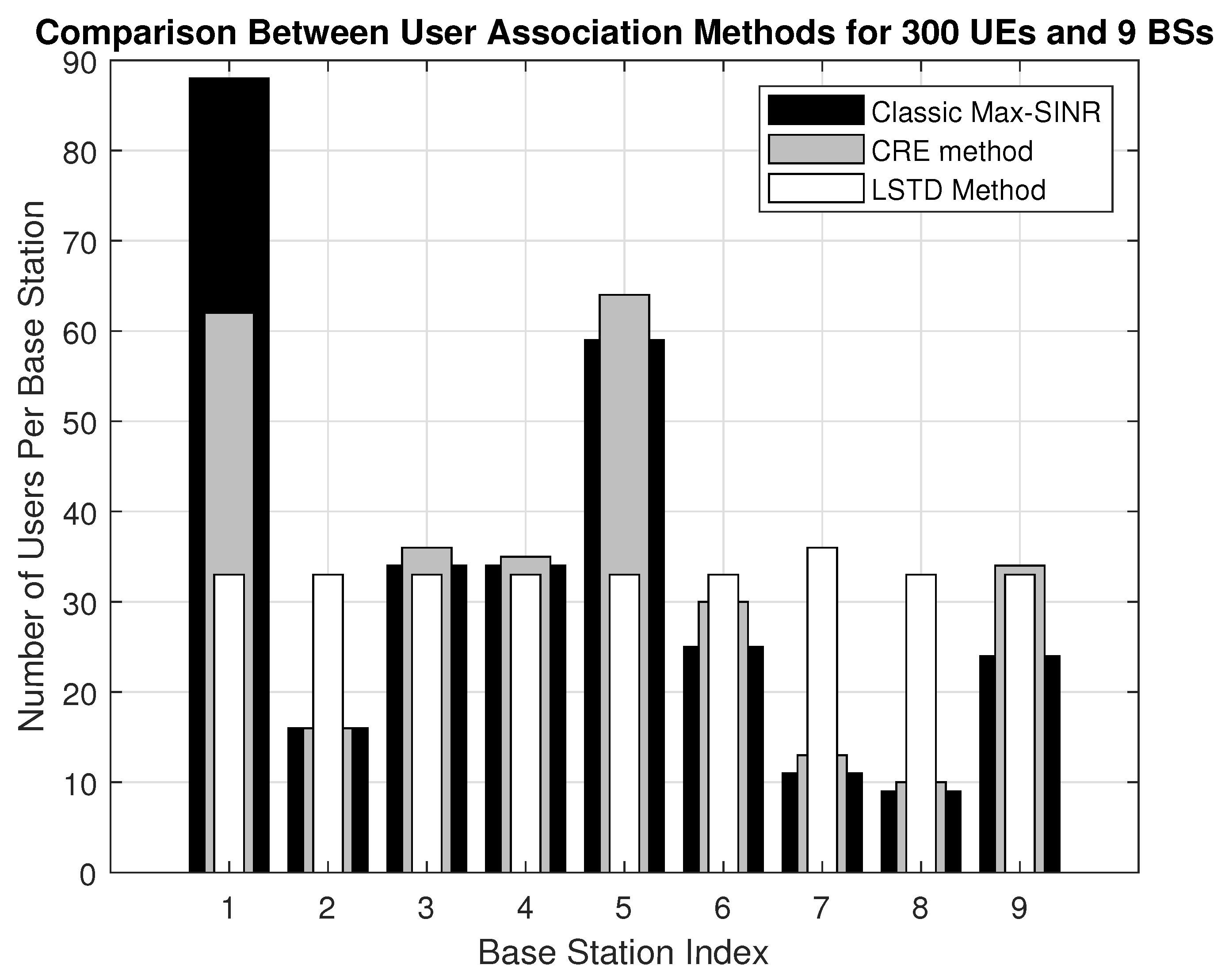
In Figure 2, we plot the load distribution for our suggested algorithm and compare it with the classic Max-SINR and other UE association algorithms. As we see, the conventional UE association methods have the shortcoming of an unbalanced load distribution and tend to associate most of UEs to the Macro BS. The CRE algorithm shows a slight improvement over Max-SINR, where Macro BS is not overloaded. It tends to withdraw the load from the Macro BS and distribute it among Micro BSs. In conventional algorithms, some BSs suffer from bandwidth shortage as they are unable to provide adequate service for all associated UEs. Link failure and poor service quality will result as a consequence of the inability of BSs to serve all their associated UEs. Conversely, optimizing the load distribution with our proposed LSTD algorithm yields a fair distribution of load among all nodes.

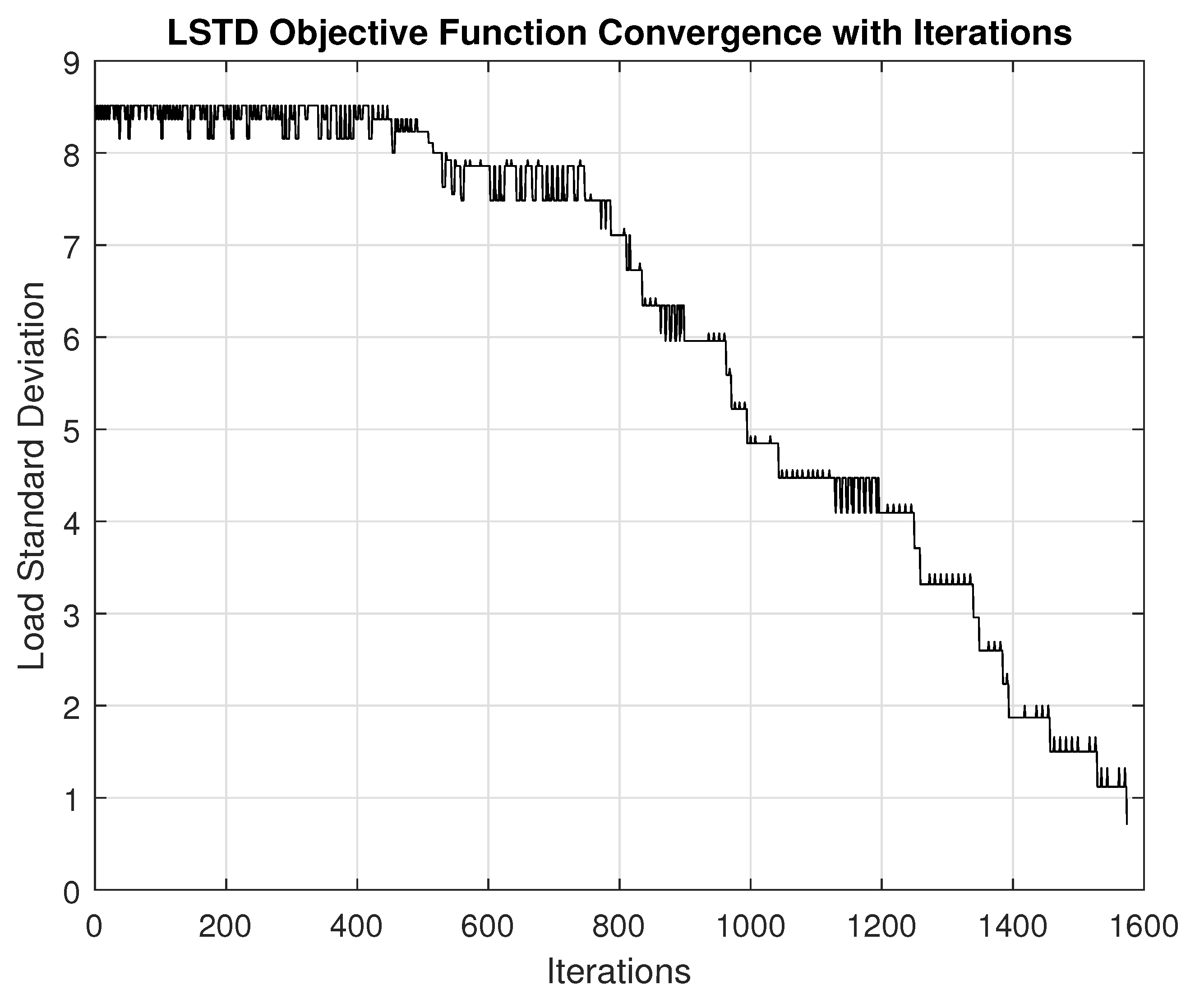
Figure 3 shows the objective function or load standard deviation as it converges. The objective function reaches the optimum load distribution (equivalent to an optimum standard deviation of 3.8406 in this situation) when a standard deviation threshold is reached, which is the closest distribution to an ideal distribution of zero that reflects that load is evenly distributed among BSs.

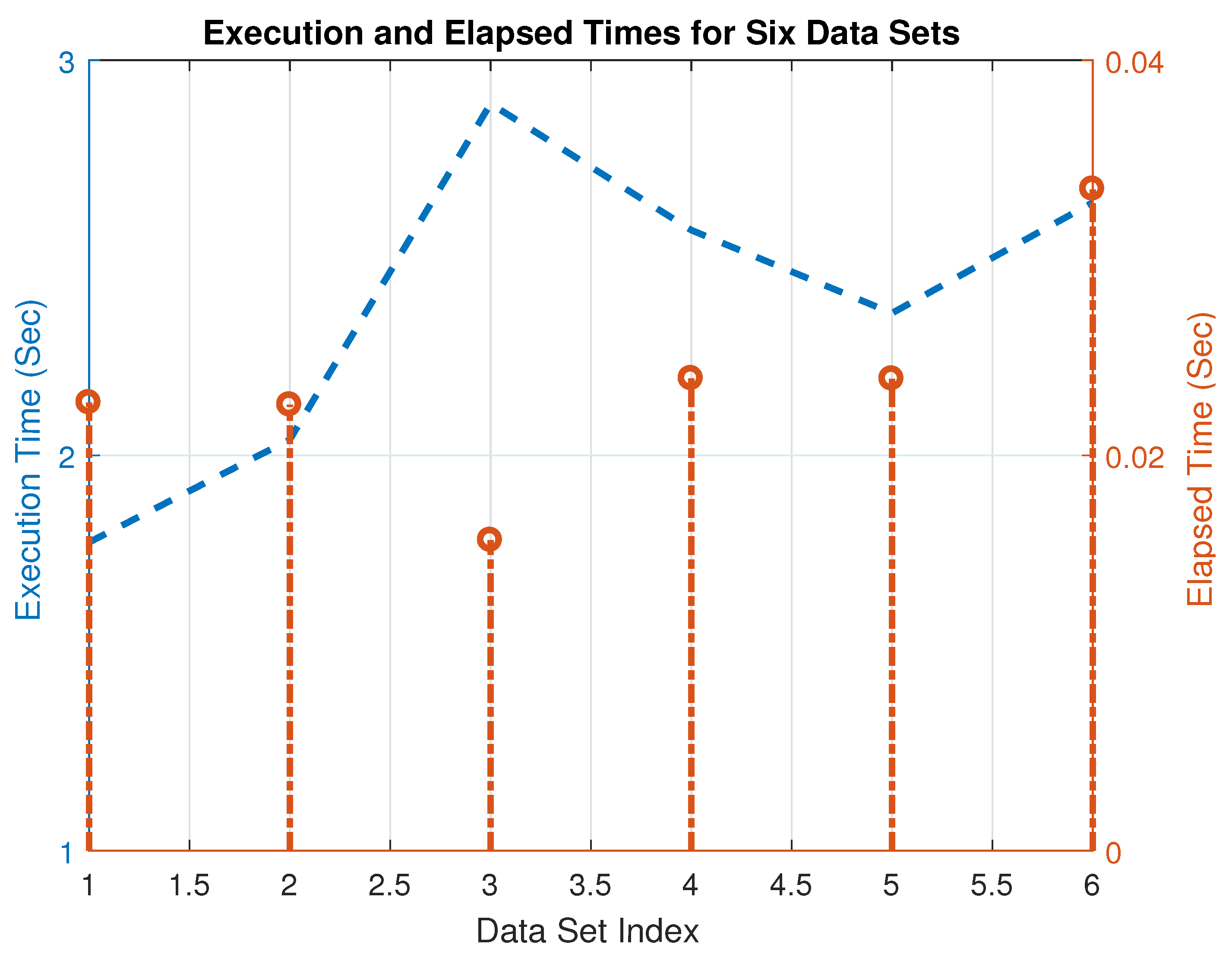
We evaluated the performance of our proposed UE association algorithm for six simulations or data sets, where cells and UEs are redistributed randomly and a different number of Macro Cells and Micro Cells are simulated. The UE association to BSs is different, and some UEs are added or dropped from the system randomly. The elapsed time is the waiting time for the query until execution (time spent by the processor) and the execution time is the actual time of the process until it is terminated. The difference between both times is spent on calculations. We plotted the execution and elapsed times for the six data sets in Figure 4. The execution time per every data set change is 2.2 s on average. We can see that the execution time is very small (compared to an average 100–150 s in [44]), so our proposed UE association algorithm is comparable to online algorithms.

Figure 5 shows rate CDF for various association techniques (AOPU and MAUM with time partitioning factor of 0.5). Max-SINR is based on signal strength, so it tends to associate UEs to Macro BSs and less low-rate UEs are available. CRE offloads some UEs from the Macro BSs and tries to balance the load using a certain bias factor. However, the optimum biasing factor is random and its exact value cannot be determined definitely. AOPU and MAUM have better performance, but our proposed algorithm provides a nearly optimum solution or equal resources for low and high-rate UEs.

Average energy efficiencies for all associated UEs is presented in Figure 6. LSTD achieves the best efficiency compared with other algorithms as it has higher data rate due to selection of the least loaded BSs in all iterations.

Coverage probability is evaluated in Figure 7 for our proposed LSTD algorithm compared to AOPU algorithm which has been improved in LSTD. The figure shows that obtained simulation and analytical results which match each other.

6. Conclusions

HetNets are gaining significant attention as they work on multiple layers, cooperating to fulfill the dream of seamless connectivity. However, appropriate UE association to BSs in HetNets is challenging as conventional algorithms do not provide fair load distribution.

In this paper, we introduced novel derivations of energy efficiency and coverage probability for a two-tier open access network. Then, we proposed an algorithm for allocating UEs to the corresponding BSs based on optimizing the standard deviation of the overall network load. The optimum goal was as close as possible to reach nearly zero standard deviation so that UE load is nearly uniform. Our algorithm enables the real-time association of mobile users to the right BS. Also, the training time, until our algorithm converges, is very small. Furthermore, our algorithm provides equal resources for low- and high-rate UEs and high data rate due to the selection of the least loaded BSs in all iterations. The feasibility of our proposed algorithm was validated with simulation results that showed excellent improvement in system performance compared to other algorithms as it improves data rate, energy efficiency, and coverage.

References

- Andrews, J.G.; Buzzi, S.; Choi, W.; Hanly, S.V.; Lozano, A.; Soong, A.C.; Zhang, J.C. What will 5G be? IEEE J. Sel. Areas Commun. 2014, 32, 1065–1082. [Google Scholar] [CrossRef]
- Ali, M.; Mumtaz, S.; Qaisar, S.; Naeem, M. Smart Heterogeneous networks: A 5G paradigm. Telecommun. Syst. 2017, 66, 311–330. [Google Scholar] [CrossRef]
- Peng, J.; Tang, H.; Hong, P.; Xue, K. Stochastic geometry analysis of energy efficiency in Heterogeneous network with sleep control. IEEE Wirel. Commun. Lett. 2013, 2, 615–618. [Google Scholar] [CrossRef]
- Altman, E.; Kumar, A.; Singh, C.; Sundaresan, R. Spatial SINR games of base station placement and mobile association. IEEE/ACM Trans. Netw. 2012, 20, 1856–1869. [Google Scholar] [CrossRef] [Green Version]
- Damnjanovic, A.; Montojo, J.; Wei, Y.; Ji, T.; Luo, T.; Vajapeyam, M.; Yoo, T.; Song, O.; Malladi, D. A survey on 3GPP heterogeneous networks. IEEE Wirel. Commun. 2011, 18, 10–21. [Google Scholar] [CrossRef]
- Dhungana, Y.; Tellambura, C. Multichannel analysis of cell range expansion and resource partitioning in two-tier heterogeneous cellular networks. IEEE Trans. Wirel. Commun. 2015, 15, 2394–2406. [Google Scholar] [CrossRef] [Green Version]
- Deb, S.; Monogioudis, P.; Miernik, J.; Seymour, J.P. Algorithms for enhanced inter-cell interference coordination (eICIC) in LTE HetNets. IEEE/ACM Trans. Netw. 2014, 22, 137–150. [Google Scholar] [CrossRef] [Green Version]
- Kong, F.; Sun, X.; Zhu, H. Optimal biased association scheme with heterogeneous user distribution in HetNets. Wirel. Pers. Commun. 2016, 90, 575–594. [Google Scholar] [CrossRef]
- Nie, X.; Wang, Y.; Zhang, J.; Ding, L. Coverage and Association Bias Analysis for Backhaul Constrained HetNets with eICIC and CRE. Wirel. Pers. Commun. 2017, 97, 4981–5002. [Google Scholar] [CrossRef]
- Kong, F.; Sun, X.; Leung, V.C.; Zhu, H. Delay-optimal biased user association in heterogeneous networks. IEEE Trans. Veh. Technol. 2017, 66, 7360–7371. [Google Scholar] [CrossRef] [Green Version]
- Zhou, T.; Liu, Z.; Qin, D.; Jiang, N.; Li, C. User Association With Maximizing Weighted Sum Energy Efficiency for Massive MIMO-Enabled Heterogeneous Cellular Networks. IEEE Commun. Lett. 2017, 21, 2250–2253. [Google Scholar] [CrossRef]
- Xu, Y.; Mao, S. User association in massive MIMO HetNets. IEEE Syst. J. 2017, 11, 7–19. [Google Scholar] [CrossRef]
- Rubio, J.; Pascual-Iserte, A.; del Olmo, J.; Vidal, J. User association strategies in HetNets leading to rate balancing under energy constraints. EURASIP J. Wirel. Commun. Netw. 2017, 2017, 204. [Google Scholar] [CrossRef] [Green Version]
- Bayat, S.; Louie, R.H.; Han, Z.; Vucetic, B.; Li, Y. Distributed user association and Femtocell allocation in Heterogeneous wireless networks. IEEE Trans. Commun. 2014, 62, 3027–3043. [Google Scholar] [CrossRef]
- Abbas, Z.H.; Muhammad, F.; Lei, J. Analysis of load balancing and interference management in heterogeneous cellular networks. IEEE Acces 2017, 5, 14690–14705. [Google Scholar] [CrossRef]
- Muhammad, F.; Abbas, Z.H.; Li, F.Y. Cell association with load balancing in nonuniform heterogeneous cellular networks: Coverage probability and rate analysis. IEEE Trans. Veh. Technol. 2017, 66, 5241–5255. [Google Scholar] [CrossRef]
- Zhou, T.; Zhao, J.; Qin, D.; Li, X.; Li, C.; Yang, L. Joint User Association and Time Partitioning for Load Balancing in Ultra-Dense Heterogeneous Networks. Mob. Netw. Appl. 2019, 1–14. [Google Scholar] [CrossRef]
- Ye, Q.; Rong, B.; Chen, Y.; Al-Shalash, M.; Caramanis, C.; Andrews, J.G. User association for load balancing in Heterogeneous cellular networks. IEEE Trans. Wirel. Commun. 2013, 12, 2706–2716. [Google Scholar] [CrossRef] [Green Version]
- Ye, Q.; Bursalioglu, O.Y.; Papadopoulos, H.C.; Caramanis, C.; Andrews, J.G. User association and interference management in massive MIMO HetNets. IEEE Trans. Commun. 2016, 64, 2049–2065. [Google Scholar] [CrossRef]
- Vu, T.K.; Bennis, M.; Samarakoon, S.; Debbah, M.; Latva-aho, M. Joint load balancing and interference mitigation in 5G Heterogeneous networks. IEEE Trans. Wirel. Commun. 2017, 16, 6032–6046. [Google Scholar] [CrossRef] [Green Version]
- Zhang, Y.; Bethanabhotla, D.; Hao, T.; Psounis, K. Near-optimal user-cell association schemes for real-world networks. In Proceedings of the 2015 Information Theory and Applications Workshop (ITA), San Diego, CA, USA, 1–6 February 2015; IEEE: Piscataway, NJ, USA, 2015; pp. 204–213. [Google Scholar]
- Hirata, A.T.; Xavier, E.C.; Borin, J.F. Optimal and heuristic decision strategies for load balancing and user association on Hetnets. In Proceedings of the 2018 IEEE Symposium on Computers and Communications (ISCC), Natal, Brazil, 25–28 June 2018; IEEE: Piscataway, NJ, USA, 2018; pp. 01143–01148. [Google Scholar]
- Bejerano, Y.; Han, S.J. Cell breathing techniques for load balancing in wireless LANs. IEEE Trans. Mob. Comput. 2009, 8, 735–749. [Google Scholar] [CrossRef]
- Navaratnarajah, S.; Dianati, M.; Imran, M.A. A novel load-balancing scheme for cellular-WLAN heterogeneous systems with a cell-breathing technique. IEEE Syst. J. 2017, 12, 2094–2105. [Google Scholar] [CrossRef] [Green Version]
- Feng, M.; Mao, S.; Jiang, T. BOOST: Base station on-off switching strategy for green massive MIMO HetNets. IEEE Trans. Wirel. Commun. 2017, 16, 7319–7332. [Google Scholar] [CrossRef]
- Hao, W.; Muta, O.; Gacanin, H.; Furukawa, H. Dynamic small cell clustering and non-cooperative game-based precoding design for two-tier heterogeneous networks with massive MIMO. IEEE Trans. Commun. 2017, 66, 675–687. [Google Scholar] [CrossRef]
- Zhong, L.; Li, M.; Cao, Y.; Jiang, T. Stable User Association and Resource Allocation Based on Stackelberg Game in Backhaul-Constrained HetNets. IEEE Trans. Veh. Technol. 2019, 68, 10239–10251. [Google Scholar] [CrossRef]
- Wu, X.; Mukherjee, B.; Chan, S.H. MACA-an efficient channel allocation scheme in cellular networks. In Proceedings of the Globecom’00-IEEE. Global Telecommunications Conference. Conference Record (Cat. No. 00CH37137), San Francisco, CA, USA, 27 November–1 December 2000; IEEE: Piscataway, NJ, USA, 2000; Volume 3, pp. 1385–1389. [Google Scholar]
- Cavalcanti, D.; Agrawal, D.; Cordeiro, C.; Xie, B.; Kumar, A. Issues in integrating cellular networks WLANs, AND MANETs: A futuristic heterogeneous wireless network. IEEE Wirel. Commun. 2005, 12, 30–41. [Google Scholar] [CrossRef]
- Yanmaz, E.; Tonguz, O.K. Dynamic load balancing and sharing performance of integrated wireless networks. IEEE J. Sel. Areas Commun. 2004, 22, 862–872. [Google Scholar] [CrossRef]
- Qiao, C.; Wu, H.; Tonguz, O. Integrated cellular and Ad hoc relay systems. IEEE Int. Conf. Comput. Commun. Netw. 2000, 19, 2105–2115. [Google Scholar]
- De, S.; Tonguz, O.; Wu, H.; Qiao, C. Integrated cellular and ad hoc relay (ICAR) systems: Pushing the performance limits of conventional wireless networks. In Proceedings of the 35th Annual Hawaii International Conference on System Sciences, Big Island, HI, USA, 10 January 2002; IEEE: Piscataway, NJ, USA, 2002; pp. 3899–3906. [Google Scholar]
- Tam, H.H.M.; Tuan, H.D.; Ngo, D.T.; Duong, T.Q.; Poor, H.V. Joint load balancing and interference management for small-cell heterogeneous networks with limited backhaul capacity. IEEE Trans. Wirel. Commun. 2016, 16, 872–884. [Google Scholar] [CrossRef] [Green Version]
- Zhou, T.; Liu, Z.; Zhao, J.; Li, C.; Yang, L. Joint user association and power control for load balancing in downlink heterogeneous cellular networks. IEEE Trans. Veh. Technol. 2017, 67, 2582–2593. [Google Scholar] [CrossRef]
- Zhuang, H.; Ohtsuki, T. A model based on Poisson point process for analyzing MIMO Heterogeneous networks utilizing fractional frequency reuse. IEEE Trans. Wirel. Commun. 2014, 13, 6839–6850. [Google Scholar] [CrossRef]
- Di Renzo, M.; Guan, P. Stochastic geometry modeling and system-level analysis of uplink heterogeneous cellular networks with multi-antenna base stations. IEEE Trans. Commun. 2016, 64, 2453–2476. [Google Scholar] [CrossRef]
- Rahimian, A.; Mehran, F. RF link budget analysis in urban propagation Microcell environment for mobile radio communication systems link planning. In Proceedings of the 2011 International Conference on Wireless Communications and Signal Processing (WCSP), Nanjing, China, 9–11 November 2011; IEEE: Piscataway, NJ, USA, 2011; pp. 1–5. [Google Scholar]
- Salh, A.; Audah, L.; Shah, N.S.M.; Hamzah, S.A. A study on the achievable data rate in massive MIMO system. In AIP Conference Proceedings; AIP Publishing LLC: Melville, NY, USA, 2017; Volume 1883, p. 020014. [Google Scholar]
- Abdul Haleem, M. On the Capacity and Transmission Techniques of Massive MIMO Systems. Wirel. Commun. Mob. Comput. 2018, 2018. [Google Scholar] [CrossRef] [Green Version]
- Dhillon, H.S.; Andrews, J.G. Downlink rate distribution in heterogeneous cellular networks under generalized cell selection. IEEE Wirel. Commun. Lett. 2013, 3, 42–45. [Google Scholar] [CrossRef] [Green Version]
- Williams, J.H. Quantifying Measurement; Morgan & Claypool Publishers: San Rafael, CA, USA, 2016. [Google Scholar]
- Chiu, S.N.; Stoyan, D.; Kendall, W.S.; Mecke, J. Stochastic Geometry and Its Applications; John Wiley & Sons: Hoboken, NJ, USA, 2013. [Google Scholar]
- Dhillon, H.S.; Ganti, R.K.; Baccelli, F.; Andrews, J.G. Modeling and analysis of K-tier downlink heterogeneous cellular networks. IEEE J. Sel. Areas Commun. 2012, 30, 550–560. [Google Scholar] [CrossRef] [Green Version]
- Keshavarz-Haddad, A.; Aryafar, E.; Wang, M.; Chiang, M. HetNets selection by clients: Convergence, efficiency, and practicality. IEEE/ACM Trans. Netw. 2016, 25, 406–419. [Google Scholar] [CrossRef]
- Ak, S.; Inaltekin, H.; Poor, H.V. Gaussian approximation for the downlink interference in Heterogeneous cellular networks. In 2016 IEEE International Symposium on Information Theory (ISIT); IEEE: Piscataway, NJ, USA, 2016; pp. 1611–1615. [Google Scholar]
- Conrad, K. The Gaussian Integral; University of Connecticut: Storrs, CT, USA, 2016; pp. 1–2. [Google Scholar]
- Singh, S.; Dhillon, H.S.; Andrews, J.G. Offloading in heterogeneous networks: Modeling, analysis, and design insights. IEEE Trans. Wirel. Commun. 2013, 12, 2484–2497. [Google Scholar] [CrossRef] [Green Version]
- Dubuc, S. An approximation of the Gamma function. J. Math. Anal. Appl. 1990, 146, 461–468. [Google Scholar] [CrossRef]
© 2020 by the authors. Licensee MDPI, Basel, Switzerland. This article is an open access article distributed under the terms and conditions of the Creative Commons Attribution (CC BY) license (http://creativecommons.org/licenses/by/4.0/).