Article

Congestion Probabilities in a Multi-Cluster C-RAN Servicing a Mixture of Traffic Sources

by
Iskanter-Alexandros Chousainov
1,
Ioannis D. Moscholios
1,* and
Panagiotis G. Sarigiannidis
2
1
Department of Informatics and Telecommunications, University of Peloponnese, 221 31 Tripolis, Greece
2
Department of Electrical and Computer Engineering, University of Western Macedonia, 501 00 Kozani, Greece
*
Author to whom correspondence should be addressed.
Electronics 2020, 9(12), 2120; https://doi.org/10.3390/electronics9122120
Submission received: 12 November 2020 / Revised: 6 December 2020 / Accepted: 9 December 2020 / Published: 11 December 2020
(This article belongs to the Special Issue Telecommunication Networks)

Abstract

:
A multi-cluster cloud radio access network (C-RAN) is considered in this paper where the remote radio heads (RRHs) form different clusters. A cluster includes RRHs that have the same radio resource unit capacity. In addition, all RRHs are separated from the common pool of computational resource units named baseband units. Each RRH accommodates calls whose arrival process can be random, quasi-random, or even bursty. The latter is modeled according to the compound Poisson process where calls arrive in the C-RAN in the form of batches whose size (in calls) is generally distributed. An arriving call requires a radio and a computational resource unit so as to be accepted in the C-RAN. If at least one of these units is not available, the call is blocked. To analyze the proposed multi-cluster C-RAN we model it as a loss system, show that the steady-state probabilities have a product form solution and propose an algorithm for the computation of congestion probabilities. The accuracy of the proposed algorithm is verified via simulation.

1. Introduction

The cloud radio access network (C-RAN) architecture consists of a number of base stations where the remote radio heads (RRHs) are separated from the baseband units (BBUs) [1]. The RRHs are grouped in different clusters according to their capacity in terms of radio resource units (RUs). On the other hand, the BBUs form a common pool of computational RUs which can be connected to the RRHs, with a high-capacity fronthaul, via the common public radio interface (CPRI) [2]. In addition, we consider virtualized BBU computational resources (V-BBU) in order to benefit from network function virtualization [1].
In this multi-cluster C-RAN architecture, we concentrate on call-level and study the main performance measure which is call blocking probabilities (CBP). A new call simultaneously requires a radio RU from the RRH that will serve that call and a computational RU from the V-BBU. If at least one of these units is not available, the call is blocked and lost. Otherwise, the new call is accepted in the RRH for an exponentially distributed service time. As far as the call arrival process is concerned, we assume that the C-RAN accommodates random, quasi-random, and bursty traffic. Random traffic refers to calls generated by an infinite number of mobile users (MUs) and is described via the classical Poisson process. It is considered to be the simplest call arrival process in teletraffic modeling due to the fact that it leads to efficient CBP formulas [3,4]. Quasi-random traffic is smoother than random traffic since it refers to calls generated by a finite number of MUs. Finally, bursty traffic, which is considered to be a dominant part in 5G networks [5,6,7], is more peaked than random traffic and can be well approximated via the compound Poisson process whose applications in loss/queueing systems are numerous [8,9,10,11,12,13]. In the compound Poisson process, batches of calls arrive in the system according to a Poisson process while their size (in number of calls) is generally distributed.
The springboard for the analysis of the proposed system is [14] where a loss model, named single-class-multi-cluster (SC-MC) model has been proposed for the case of random traffic only. The term ‘single-class’ refers to the fact that all new calls have the same requirements in terms of RUs. The authors of [14] consider a multidimensional Markov chain for the description of the SC-MC loss model. This chain is reversible, a fact that leads to the computation of the steady-state probabilities via a product form solution (PFS). The latter leads to an accurate CBP calculation via recursive formulas or via an evaluation method which requires the system’s state space enumeration/processing. Recently, in [15], the SC-MC model has been extended to include the case of quasi-random traffic, only. We name this model finite SC-MC (f-SC-MC) model.
In this paper, we generalize the SC-MC and the f-SC-MC models by assuming that RRHs may serve random, quasi-random and bursty traffic. The proposed model is named generalized SC-MC (g-SC-MC) model while our contribution can be summarized as follows: (1) we initially show that the g-SC-MC model can be analytically described via a continuous time Markov chain and that the steady-state probabilities have a PFS, (2) we determine the congestion probabilities via a brute force (BF) evaluation method, (3) we propose a convolution algorithm for the efficient determination of congestion probabilities in the multi-cluster C-RAN, and (4) we provide a comparison of the analytical results of the g-SC-MC model with those obtained according to the models of [14,15] and verify the accuracy of the proposed convolution algorithm via simulation.
Generally speaking, it is significant in network planning and dimensioning procedures to have convolution algorithms or efficient recursive formulas for the determination of various performance measures including congestion probabilities [16,17,18,19,20,21,22,23,24,25,26,27,28,29,30,31,32,33,34,35,36]. We focus on convolution algorithms which are adopted in the literature both in PFS [37,38,39] and in non-PFS queueing/loss models [40,41,42]. The advantage of such algorithms is that they can incorporate various resource sharing policies such as the bandwidth reservation policy, the complete sharing policy, as well as threshold-based policies [43,44,45,46].
The organization of this paper is as follows: In Section 2, we present a short review of the SC-MC model and provide a convolution algorithm for the CBP determination. In Section 3, we propose the g-SC-MC model. In Section 3.1, we present a PFS for the determination of the steady-state probabilities while in Section 3.2 and Section 3.3 we propose a BF method and a convolution algorithm for the calculation of congestion probabilities, respectively. In Section 4, we provide analytical and simulation results for the congestion probabilities of the proposed g-SC-MC model and the SC-MC model of [14]. We present our conclusion in Section 5. In Appendix A, we provide a short tutorial example of the necessary congestion probabilities calculations for the proposed g-SC-MC model.

2. The SC-MC Model—A Review

Consider the multi-cluster C-RAN of Figure 1 where the V-BBU and the RRHs are separated. In this network, Z classes of RRHs are considered. Class z (z = 1, …, Z) forms a cluster of RRHs that includes a total number of Mz RRHs. A RRH of class z has a capacity of Cz radio RUs which serve the Poisson arriving calls of the MUs. Similarly, the V-BBU consist of T computational RUs.
Let λz be the rate of Poisson arriving calls in a class z RRH. A call is accepted for a generally distributed service time with mean μ−1 in a RRH if a radio RU (from that RRH) as well as a computational RU are available when the call arrives in the system. Otherwise, call blocking occurs. The corresponding offered traffic-load in a class z RRH is given by α z = λ z / μ (in erl).
Consider the m-th RRH of class z (z = 1, …, Z and m = 1, …, Mz) and let nz,m be the calls under service in that particular RRH. Then, the steady-state vector n = ( n 1 , 1 ,   , n 1 , M 1 , , n z , 1 ,   , n z , M z , , n Z , 1 , , n Z , M Z ) expresses the number of calls serviced in the RRHs of the Z classes while P ( n ) is the corresponding steady-state probability distribution. The latter has the following PFS [14]
P ( n ) = G 1 ( z = 1 Z m = 1 M z α z n z , m / n z , m ! ) ,
where G = n Ω ( z = 1 Z m = 1 M z α z n z , m / n z , m ! ) and Ω is the system’s state space described as follows Ω = { n : 0 n z , 1 , , n z , M z C z ,     0 z = 1 Z m = 1 M z n z , m T } .
Based on (1), we compute the total CBP of calls in a class z RRH, Bz,tot, as
B z , t o t = B c + B z , r ,
where Bc refers to the blocking caused due to insufficient computational RUs while Bz,r expresses the blocking caused solely due to unavailability of radio RUs.
According to [14], the case of simultaneous blocking due to both insufficient radio and computational RUs is classified as Bc. In that sense, the sets Ac and Az,r that include the blocking states of Bc and Bz,r, respectively, are mutually exclusive, i.e., A c A z , r = . We also keep this distinction in the proposed g-SC-MC model.
The values of Bz,tot can be accurately (compared to simulation) calculated either via a BF method (helpful only in small multi-cluster C-RAN examples since it requires enumeration/processing of the system’s state space Ω ) or via a recursive method [14]. Some minor corrections in the CBP formulas of [14] have been presented in [15].
Alternatively, the values of Bz,tot together with the occupancy distribution of the computational RUs can be efficiently determined via the following convolution algorithm [15]:
  • Step 1
For each of the Mz RRHs that belong to class z (z = 1, …, Z and m = 1, …, Mz) determine the occupancy distribution q z , m ( j ) , where j = 1, …, Cz, via
q z , m ( j ) = α z j j !   q z , m ( 0 ) .
The normalization of q z , m ( j ) can be achieved via the constant G z , m = j = 0 C z q z , m ( j ) and in that case the normalized values become q z , m ( j ) = q z , m ( j ) / G z , m .
  • Step 2
Compute the aggregated occupancy distribution Q(−(z,1)) of all RRHs, excluding the (z, 1) RRH, via the formula
Q ( - ( z , 1 ) ) = q 1 , 1 * * q 1 , M 1 * * q z , 2 * * q z , M z * * q Z , 1 * * q Z , M Z ,
where the first part of (4) ( q 1 , 1 * * q 1 , M 1 ) refers to the M1 RRHs of the first class, the second part ( q z , 2 * * q z , M z ) refers to the Mz − 1 RRHs of the zth class (the (z, 1) RRH is excluded) and the last part ( q Z , 1 * * q Z , M Z ) refers to the MZ RRHs of the Zth class while
q z , u * q z , w = { q z , u ( 0 ) q z , w ( 0 ) ,     x = 0 1 q z , u ( x ) q z , w ( 1 x ) , , x = 0 T q z , u ( x ) q z , w ( T x ) } .
Since the resulting distribution may not be normalized, it is recommended to apply the normalization constant G z , u , w in the results of (5).
  • Step 3
Compute Bz,tot based on the results of the previous step
B z , t o t = B z , r + B c = G 1 ( q z , 1 ( C z ) r = 0 T C z 1 Q ( ( z , 1 ) ) ( r ) + q ( T ) ) ,
where q z , 1 ( C z ) expresses the unavailability of radio RUs in the (z, 1) RRH (computed in step 1), Q ( ( z , 1 ) ) ( r ) express the normalized values of Q ( ( z , 1 ) ) ( r ) and q ( T ) expresses the un-normalized probability of unavailable computational RUs, obtained via q ( T ) = r = 0 T Q ( - ( z , 1 ) ) ( r ) q z , 1 ( T - r ) while G is the (normalization) constant of the operation Q ( - ( z , 1 ) ) * q z , 1 calculated in (5).
Note that (14) refers to the Bz,tot of any RRH that belongs to class z since all RRHs of that class have offered traffic-load az and capacity Cz.
Based on the presented algorithm, we compute the computational RUs’ occupancy distribution according to the formulas
q ( 0 ) = G 1 ( Q ( ( z , 1 ) ) ( 0 ) q z , 1 ( 0 ) ) ,                                           j = 0 q ( j ) = G 1 ( r = 0 j Q ( ( z , 1 ) ) ( r ) q z , 1 ( j r ) ) ,           j = 1 , , T
where G expresses the normalization constant of Q ( - ( z , 1 ) ) * q z , 1 .

3. Proposed g-SC-MC Model

3.1. Description of the Analytical Model

In the proposed g-SC-MC model, we consider again a multi-cluster C-RAN which consists of the V-BBU (T computational RUs) and Z classes of RRHs. Class z (z = 1, …, Z) consists of a cluster of RRHs that includes a total number of Mz RRHs whose capacity is Cz radio RUs. Let the number of Mz RRHs be composed of Mz,inf RRHs that serve random traffic, Mz,fin RRHs that accommodate quasi-random traffic and Mz,cP RRHs that accommodate compound Poisson traffic, i.e., Mz,inf + Mz,fin + Mz,cP = Mz.
In the case of random traffic, let λz,P be the rate of Poisson arriving calls in the (z, m) RRH (m = 1, …, Mz,inf and z = 1, …, Z). The corresponding offered traffic-load will be α z , P = λ z , P / μ . In the case of quasi-random traffic, let λ z , m , F = ( N z , m n z , m ) v z , m , F be the call arrival rate in the (z, m) RRH (m = Mz,inf + 1,…, Mz,inf + Mz,fin and z = 1, …, Z) where Nz,m denotes the population of MUs that can generate traffic in the (z, m) RRH, nz,m refers to the in-service calls in that RRH and vz,m,F expresses the call arrival rate per idle MU. In the case of the compound Poisson process, batches of calls arrive in the (z, m) RRH (m = Mz,inf + Mz,fin + 1, …, Mz and z = 1, …, Z) according to a Poisson process, with arrival rate λz,cP, while the batch size (in number of calls) is generally distributed. Calls that belong to the same arriving batch are treated independently which means that some calls can be accepted in the serving RRH while the rest calls will be blocked, depending on the availability of RUs.
As far as the call admission is concerned, a call is accepted for an exponentially distributed service time with mean μ−1 in a RRH if a radio RU (from that RRH) as well as a computational RU are available when the call arrives in the system. Otherwise, call blocking occurs.
Let the steady-state vector n = ( n 1 , 1 ,   , n 1 , M 1 , , n z , 1 ,   , n z , M z , , n Z , 1 , , n Z , M Z ) express the number of in-service calls in the RRHs of the Z classes, where M1 = M1,inf + M1,fin + M1,cP, Mz = Mz,inf + Mz,fin + Mz,cP and MZ = MZ,inf + MZ,fin + MZ,cP. The corresponding steady-state probability distribution is denoted as P gen ( n ) . In order to analyze the g-SC-MC model, we show that P gen ( n ) can be described via a PFS. To this end, it should be shown that some form of local balance exists between state n and state n z , m + = ( n 1 , 1 ,   , n z , m + 1 , , n Z , M Z ) . More specifically, consider the level L n ( z , m ) that separates state n z , m + from state n . This level is crossed if one of the following three call-arrival cases occurs: (i) an arriving call that follows a Poisson process requests service from the (z, m) RRH (where m = 1,…, Mz,inf), (ii) an arriving call that follows a quasi-random process requests service from the (z, m) RRH (where m = Mz,inf + 1,…, Mz,inf + Mz,fin), (iii) calls of an arriving batch requests service from the (z, m) RRH (where m = Mz,inf + Mz,fin + 1, …, Mz). An additional call-departure case exists when an in-service call departs from the serving RRH after its service is completed. In what follows, we focus on each of the three call-arrival cases and the corresponding call-departure case.
In the first case, we have a Poisson arriving call of rate λz,P in the (z, m) RRH (m = 1, …, Mz,inf and z = 1, …, Z). We can express the upward probability flow across L n ( z , m ) as
f ( u p ) ( L n ( z , m ) ) = λ z , P P gen ( n ) .
The downward probability flow across L n ( z , m ) takes place when a call departs from the (z, m) RRH and can be expressed as
f ( d o w n ) ( L n ( z , m ) ) = ( n z , m + 1 ) μ P gen ( n z , m + ) .
Based on (8) and (9), we have the following local balance equation for L n ( z , m )
λ z , P P gen ( n ) = ( n z , m + 1 ) μ P gen ( n z , m + ) .
In the second case, we have an arriving call, generated from a finite number of MUs, in the (z, m) RRH (m = Mz,inf + 1, …, Mz,inf + Mz,fin and z = 1, …, Z). We can express the upward probability flow across L n ( z , m ) as
f ( u p ) ( L n ( z , m ) ) = λ z , m , F P gen ( n ) = ( N z , m n z , m ) v z , m , F P gen ( n ) .
The corresponding downward probability flow across L n ( z , m ) can be expressed via (9). Based on (11) and (9), we have the following local balance equation for L n ( z , m )
( N z , m n z , m ) v z , m , F P gen ( n ) = ( n z , m + 1 ) μ P gen ( n z , m + ) .
In the third case, we have an arriving batch of calls in the (z, m) RRH (m = Mz,inf + Mz,fin + 1, …, Mz and z = 1, …, Z). We can express the upward probability flow across L n ( z , m ) as
f ( u p ) ( L n ( z , m ) ) = ω = 0 n z , m P gen ( n z , m ω ) λ z , cP r = ω + 1 S r ,
where n z , m ω = ( n 1 , 1 ,   , n z , m - ω , , n Z , M Z ) , P gen ( n z , m ω ) is the steady-state probability and Sr is the probability that the arriving batch contains r calls.
The corresponding downward probability flow across L n ( z , m ) can be expressed via (9). Based on (13) and (9), we have the following local balance equation for L n ( z , m )
ω = 0 n z , m P gen ( n z , m ω ) λ z , cP r = ω + 1 S r = ( n z , m + 1 ) μ P gen ( n z , m + ) .
Equations (10), (12), and (14) can be satisfied via the following PFS
P gen ( n ) = G 1 ( z = 1 Z m = 1 M z , inf α z , P n z , m n z , m !   m = M z , inf + 1 M z , inf + M z , fin ( N z , m   n z , m )   α z , m ,     idle n z , m m = M z , inf + M z , fin + 1 M z P n z , m ( z , m ) ) ,
where G = n Ω ( z = 1 Z m = 1 M z , inf α z , P n z , m n z , m !   m = M z , inf + 1 M z , inf + M z , fin ( N z , m   n z , m )   α z , m ,     idle n z , m m = M z , inf + M z , fin + 1 M z P n z , m ( z , m ) ) , Ω is described as Ω = { n : 0 n z , 1 , , n z , M z C z ,     0 z = 1 Z m = 1 M z n z , m T } , α z , m , idle = v z , m , F / μ expresses the offered traffic-load per idle MU, P n z , m ( z , m ) = ω = 1 n z , m α z , cP n z , m P n z , m ω ( z , m ) S ^ ω - 1 , α z , cP = λ z , cP / μ and S ^ ω = r = ω + 1 S r is the complementary batch size distribution.
Having determined the values of P gen ( n ) we can compute the total time congestion (TC) probabilities in the (z, m) RRH (m = 1, …, Mz and z = 1, …, Z) either according to a BF method or according to a convolution algorithm (presented in Section 3.2 and Section 3.3, respectively) and based on the formula
B z , m , t o t T C = B c T C + B z , m , r T C ,
where B c T C and B z , m , r T C refer to the unavailable computational RUs in the V-BBU and radio RUs in the (z, m) RRH, respectively.

3.2. BF Method for the Computation of Congestion Probabilities

The determination of B c T C can be based on the values of P gen ( n ) according to the formula
B c T C = n Ω = Τ P gen ( n ) ,
where Ω = Τ = { n : z = 1 Z m = 1 M z n z , m = T } .
On the same hand, the values of B z , m , r T C can be computed (via (15)) via
B z , m , r T C = n Ω < Τ z , m , C z P gen ( n ) ,
where Ω < Τ z , m , C z = { Ω z , m , C z Ω < Τ } ,     Ω z , m , C z = { n : n z , m = C z } ,     Ω < Τ = { n : z = 1 Z m = 1 M z n z , m < T } .
It is evident that (17) and (18) can be quite complex since it is expected to enumerate and process the state space Ω. Because of this, we adopt the convolution algorithm proposed in the next subsection.

3.3. Convolution Algorithm for the Computation of Congestion Probabilities

The PFS of the g-SC-MC model implies that a convolution algorithm can be applied for the accurate and efficient determination of congestion probabilities. To this end, we propose the following three-step convolution algorithm.
  • Step 1
(a) For each of the Mz,inf RRHs that accommodate random traffic and belong to class z (z = 1, …, Z and m = 1, …, Mz,inf) determine the occupancy distribution q gen , z , m ( j ) , where j = 1, …, Cz, via
q gen , z , m ( j ) = α z , P j j !   q gen , z , m ( 0 ) .
(b) For each of the Mz,fin RRHs that accommodate quasi-random traffic and belong to class z (z = 1, …, Z and m = Mz,inf + 1, …, Mz,inf + Mz,fin) determine the occupancy distribution q gen , z , m ( j ) , where j = 1, …, Cz, via
q gen , z , m ( j ) = ( N z , m       j )   α z , m ,     idle j q gen , z , m ( 0 ) .
(c) For each of the Mz,cP RRHs that accommodate compound Poisson traffic and belong to class z (z = 1, …, Z and m = Mz,inf + Mz,fin + 1, …, Mz) determine the occupancy distribution q gen , z , m ( j ) , where j = 1, …, Cz, according to the formula
q gen , z , m ( j ) = l = 1 j α z , cP j q gen , z , m ( j - l ) S ^ l - 1 .
Note that q gen , z , m ( 0 ) = 1 while q gen , z , m ( x ) = 0 for x > C or x < 0. Furthermore, the normalization of q gen , z , m ( j ) can be achieved via the constant G gen , z , m = j = 0 C z q gen , z , m ( j ) and in that case the normalized values become q gen , z , m ( j ) = q gen , z , m ( j ) / G gen , z , m .
  • Step 2
Compute the aggregated occupancy distribution Qgen,(−(z,m)) of all RRHs, excluding the (z, m) RRH, via the formula
Q gen , ( - ( z , m ) ) = q gen , 1 , 1 * * q gen , 1 , M 1 * * q gen , z , 1 * * q gen , z , m 1 * q gen , z , m + 1 * * q gen , z , M z * * q gen , Z , 1 * * q gen , Z , M Z ,
where
q gen , z , u * q gen , z , w = { q gen , z , u ( 0 ) q gen , z , w ( 0 ) ,     x = 0 1 q g e n , z , u ( x ) q g e n , z , w ( 1 x ) , , x = 0 T q g e n , z , u ( x ) q g e n , z , w ( T x ) } .
Since the resulting distribution may not be normalized, it is recommended to apply the normalization constant G gen , z , u , w in the results of (23).
  • Step 3
Compute B z , m , t o t T C based on the results of Step 2
B z , m , t o t T C = B z , m , r T C + B c T C = G gen 1 ( q gen , z , m ( C z ) r = 0 T C z 1 Q gen , ( - ( z , m ) ) ( r ) + x = 0 T Q gen , ( - ( z , m ) ) ( x ) q gen , z , m ( T - x ) ) ,
where q gen , z , m ( C z ) expresses the unavailability of radio RUs in the (z, m) RRH (computed in the first step), while the second summation expresses the un-normalized probability of unavailable computational RUs and Ggen is the normalization constant of Q gen , ( - ( z , m ) ) * q gen , z , m computed via (23).
In addition to TC probabilities (which refer to the proportion of time the multi-cluster C-RAN has no available RUs) we can also compute the call congestion (CC) probabilities (which refer to the proportion of lost calls), B z , m C C , for a new call in an RRH that accommodates quasi-random or compound Poisson traffic. CC and TC probabilities coincide in the case of random traffic. To determine the CC probabilities in the case of quasi-random traffic, we can adopt the convolution algorithm for a system with Nz,m−1 sources. On the same hand, to determine the CC probabilities in the case of compound Poisson traffic we can adopt the formula
B z , m C C = α z , cP S ^ n ¯ z , m α z , cP S ^ ,
where S ^ = l = 1 l S ^ l is the average batch size (in number of calls) and n ¯ z , m refers to the average number of calls accommodated in the (z, m) RRH.
A popular batch size distribution is the geometric distribution which possesses the memoryless property [4,47]. If this distribution is adopted and assuming that β is its parameter, then S ^ = 1 / ( 1 β ) .
The determination of n ¯ z , m can be based on the formula
n ¯ z , m = 1 G gen j = 1 C z y gen , z , m ( j ) q gen , z , m ( j ) r = 0 T j Q gen , ( - ( z , m ) ) ( r ) ,
where Ggen is the normalization constant of the convolution operation Q gen , ( - ( z , m ) ) * q gen , z , m determined via (23) and y gen , z , m ( j ) expresses the average number of calls that exist in state j of the (z, m) RRH.
The determination of y gen , z , m ( j ) , for j = 1, …, Cz, can be based on the formula
y gen , z , m ( j ) = α z , cP q gen , z , m ( j ) l = 1 j q gen , z , m ( j - l ) S ^ l - 1 ,
Based on the convolution algorithm, we can also compute the computational RUs’ occupancy distribution according to the formulas
q gen ( 0 ) = Q g e n , ( ( z , m ) ) ( 0 ) q gen , z , m ( 0 ) / G gen ,                                           j = 0 q gen ( j ) = r = 0 j Q g e n , ( ( z , m ) ) ( r ) q g e n , z , m ( j r ) / G gen ,           j = 1 , , T
Considering the computational complexity of (23) is in the order of O(T2) while the corresponding complexity of (28) is in the order of O(MT2), where M = (M1, …, MZ).

4. Evaluation

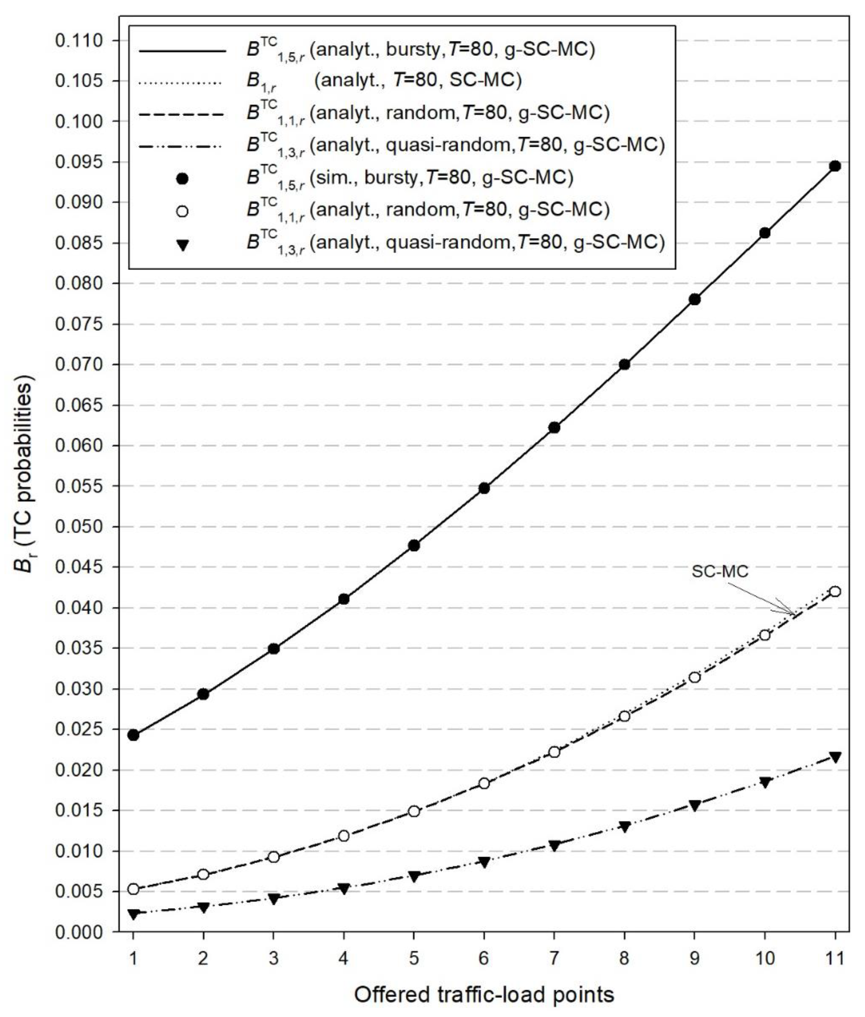
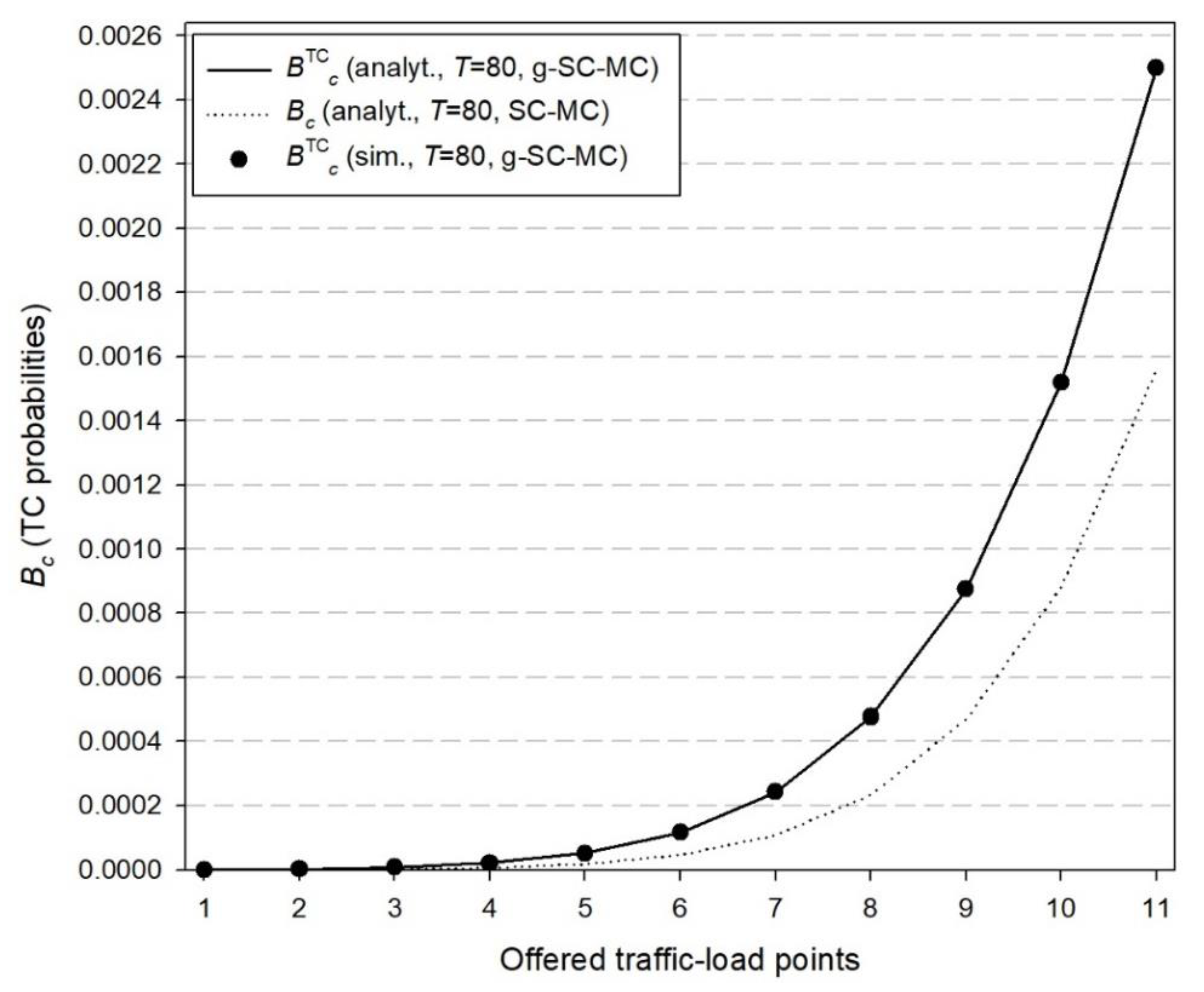
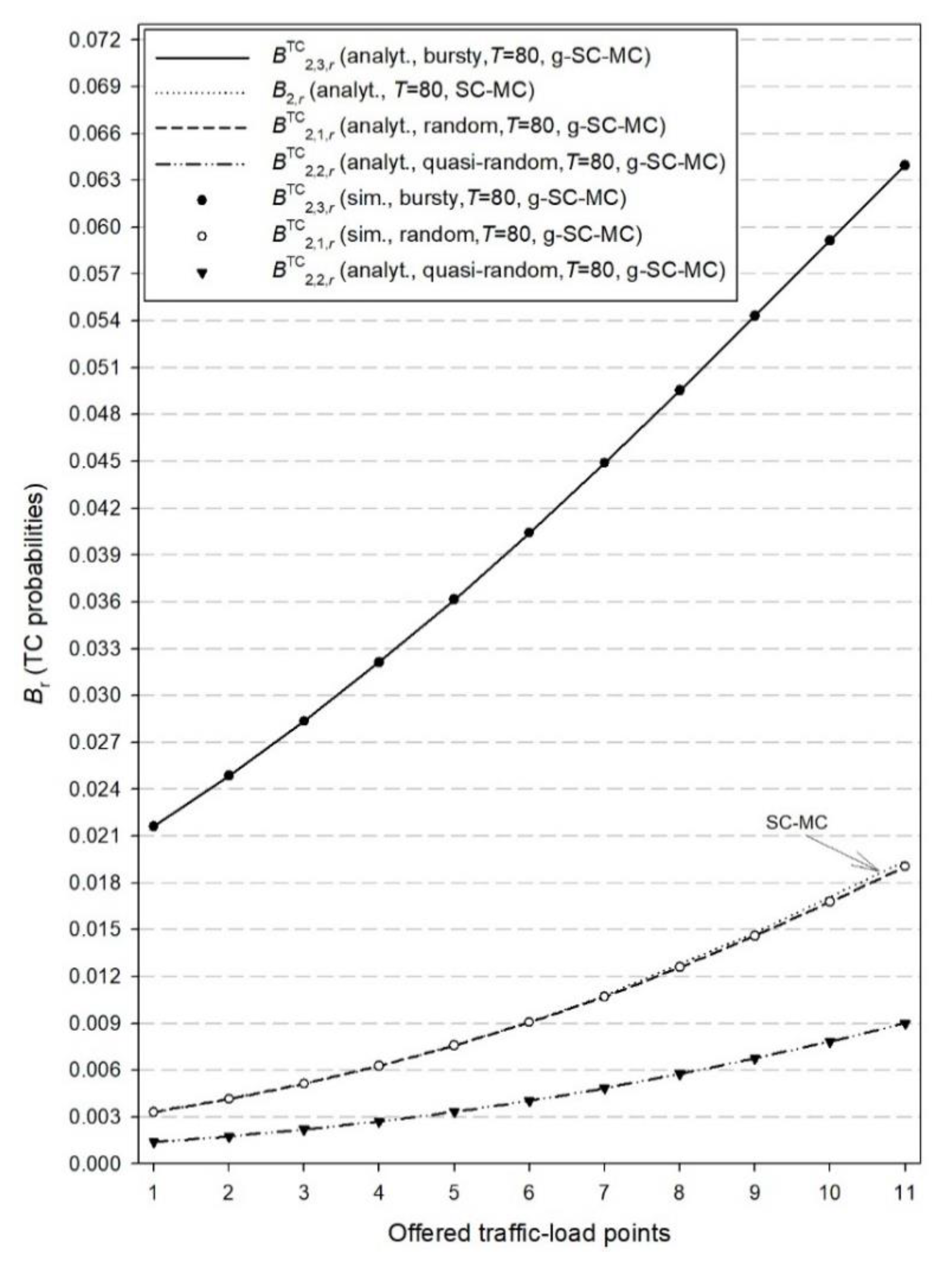
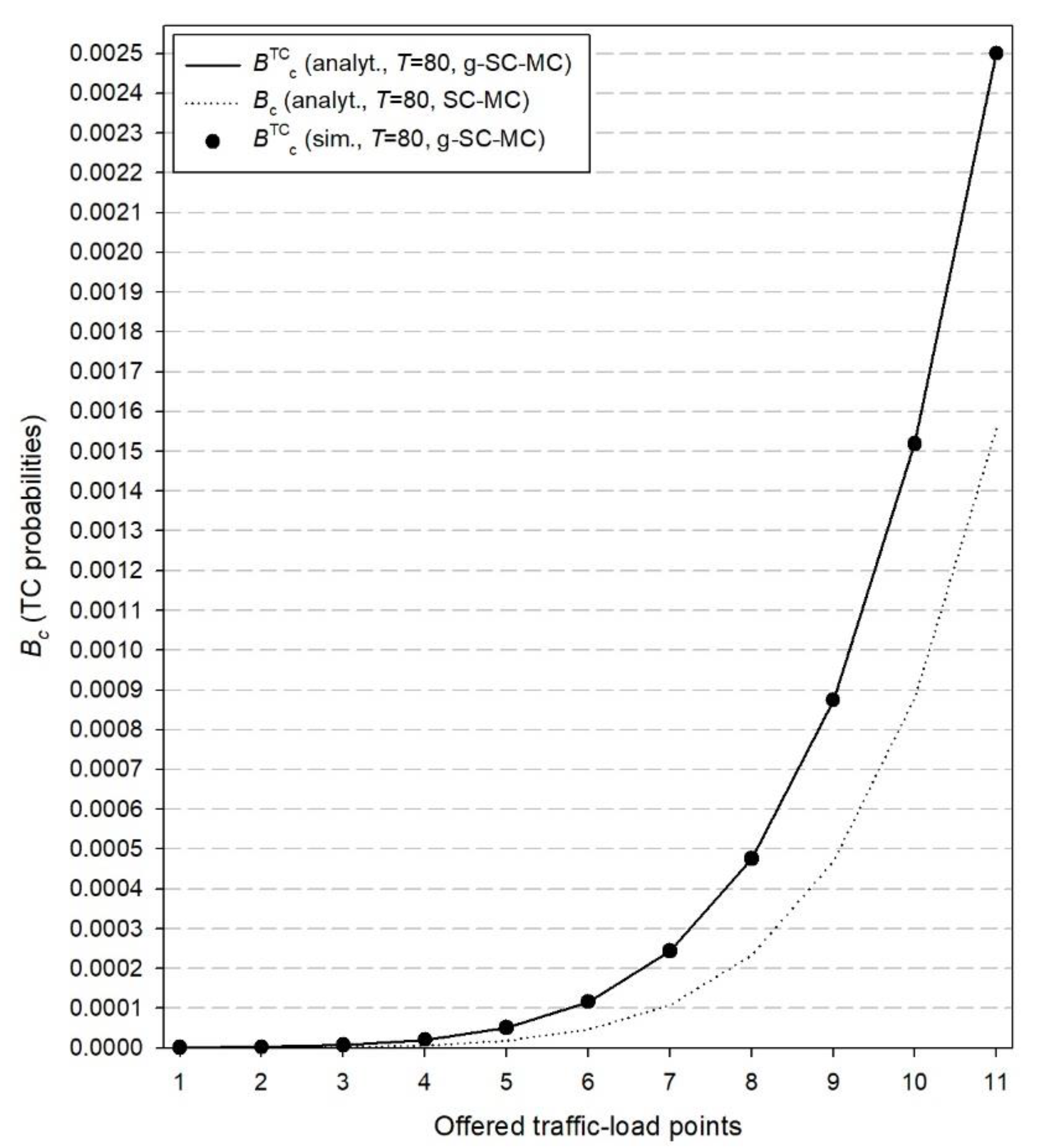
In this section, we consider an example of a multi-cluster C-RAN and provide both simulation and analytical results for the CC and TC probabilities in the case of the proposed g-SC-MC model and analytical results for the existing SC-MC model. The simulation tool adopted in our example is SIMSCRIPT III [48] while all simulation results are mean values of seven runs. In every run, 200 million calls are generated while the initial 5% of them are not taken into consideration in order to have a warm-up period [49,50]. Regarding reliability ranges, they are less than two order of magnitudes and therefore we do not present them in Figure 2, Figure 3, Figure 4, Figure 5, Figure 6 and Figure 7.
The C-RAN example presented herein consists of two clusters (Z = 2). The first cluster consists of M1 = 6 RRHs where the capacity per RRH is C1 = 10 radio RUs. The second cluster consists of M2 = 3 RRHs where the capacity per RRH is C2 = 15 radio RUs. Regarding the computational RUs, we consider that T = 80 RUs. Values of T that are much lower than T = M1C1 + M2C2 = 105 RUs will result in quite high values for the congestion probabilities due to insufficient computational RUs ( B c T C ) and therefore are not taken into consideration herein. In the case of the existing SC-MC model, we assume that the offered traffic load (per RRH) in the first cluster is α 1 = 4 erl and in the second cluster α 2 = 7 erl. In the case of the proposed g-SC-MC model, the traffic-load offered in the RRHs of the first cluster is as follows: the first two RRHs accommodate random traffic with α 1 , P = 4 erl (per RRH), RRHs numbered 3 to 4 accommodate quasi-random traffic with N 1 , 3 = N 1 , 4 = 50 sources and α 1 , 3 , idle = α 1 , P / N 1 , 3 , α 1 , 4 , idle = α 1 , P / N 1 , 4 while RRHs numbered 5 to 6 accommodate compound Poisson traffic with α 1 , cP = 4 erl. Regarding the size distribution (in terms of calls) of the arriving batches, we consider the geometric distribution with parameter β = 0.2. Similarly, the traffic-load offered in the RRHs of the second cluster is as follows: the first RRH accommodates random traffic with α 2 , P = 7 erl, the second RRH accommodates quasi-random traffic with N 2 , 2 = 100 sources and α 2 , 2 , idle = α 2 , P / N 2 , 2 while the third RRH accommodates compound Poisson traffic with α 2 , cP = 7 erl and a geometrically batch size distribution with β = 0.2.
In the x-axis of Figure 2, Figure 3, Figure 4, Figure 5, Figure 6 and Figure 7, the values of offered traffic-load increase in steps of 0.2 erl. Therefore, for Figure 2, Figure 3 and Figure 4 that refer to the first cluster, point 1 in the x-axis is 4 erl while point 11 is 6.0 erl. Similarly, for Figure 5, Figure 6 and Figure 7 that refer to the second cluster, point 1 in the axis is 7 erl while point 11 is 9.0 erl.
In Figure 2, we present both simulation and analytical results of the TC probabilities ( B 1 , m , r T C ) for the g-SC-MC model and the corresponding results ( B 1 , r ) for the SC-MC model, which refer to time congestion due to unavailability of radio RUs. In Figure 3, we present simulation and analytical results of the TC probabilities ( B c T C ) for the g-SC-MC model and the corresponding results ( B c ) for the SC-MC model, which refer to time congestion due to unavailability of computational RUs. Finally, in Figure 4, we present simulation and analytical results of the CC probabilities ( B 1 , m C C ) for the g-SC-MC model and the corresponding results ( B 1 , t o t B 1 C C ) for the SC-MC model. According to Figure 2, Figure 3 and Figure 4, we observe that: (i) simulation and analytical results are quite close in the proposed g-SC-MC model, (ii) all congestion probabilities increase as the offered traffic-load increases, (iii) the choice of T = 80 RUs results in an increase of B c T C and B c especially for higher values of the offered traffic-load (in the case of T = M1C1 + M2C2 = 105 RUs, both B c T C and B c can be considered negligible), and (iv) the existing SC-MC model cannot capture the behavior of the proposed g-SC-MC model since the former accommodates only random traffic and not bursty or quasi-random traffic. This failure is depicted even for a small value of β. Higher values of β will increase the difference between the results obtained via the two models.
Similar conclusions are obtained in Figure 5, Figure 6 and Figure 7 which refer to the congestion probabilities in the RRHs of the second cluster. As a final comment, we mention that the accuracy of the analytical results of the proposed model, compared to simulation, is not affected by an increase in the number of clusters.

5. Conclusions

We proposed a loss model for the analysis and evaluation of a multi-cluster C-RAN that accommodates random, quasi-random, and bursty traffic. New calls can be accepted in an RRH if their resource requirements (a radio and a computational RU) can be met. If any of these two RUs is not available, then call blocking occurs. We showed that the model has a PFS for the steady-state probabilities and provided an efficient convolution algorithm for the computation of the main performance measures such as congestion probabilities. The accuracy of the proposed algorithm was verified via simulation. As a possible future extension of this work, we intend to study single or multi-cluster C-RAN that accommodates calls: (i) whose RUs may fluctuate between a maximum and a minimum value during this service time, forming the so called “elastic traffic” [51,52,53,54,55]; or (ii) whose requirements in terms of RUs may be different during the call admission phase [56,57,58].

Author Contributions

Conceptualization, all authors; Methodology, all authors; Software, I.-A.C. and I.D.M.; Validation, I.-A.C. and I.D.M.; Writing—original draft preparation, all authors; Writing—review and editing, all authors. All authors have read and agreed to the published version of the manuscript.

Funding

This research received no external funding.

Conflicts of Interest

The authors declare no conflict of interest.

Appendix A

In this appendix, a tutorial example is presented that shows some intermediate results required for the determination of congestion probabilities in the proposed g-SC-MC model. To this end, we consider a multi-cluster C-RAN of T = 7 computational RUs and Z = 2 classes of RRHs. The first class consists of M1 = 2 RRHs of C1 = 3 radio RUs. The second class consists of M2 = 1 RRH of C2 = 4 radio RUs. Regarding the first class, arriving calls in the first RRH follow a Poisson process with rate λ1,P = 1.0, while arriving calls in the second RRH follow a quasi-random process with N 1 , 2 =10 and v 1 , 2 , F =0.1. Regarding the second class, arriving calls in the RRH follow a compound Poisson process with λ 2 , cP = 0.8 and β = 0.5. The service time of all calls is exponentially distributed with mean μ−1 = 1.0. The state space of this example consists of 70 states (whose form is n = ( n 1 , 1 ,   n 1 , 2 , n 2 , 1 ) ).
The application of the proposed convolution algorithm in this example is as follows:
  • Step 1
    • For z = 1, m = 1 and j =1, …, 3 compute q gen , 1 , 1 ( j ) assuming that α 1 , P = 1.0:
      j = 1 q gen , 1 , 1 ( 1 ) = α 1 , P 1 1 ! q gen , 1 , 1 ( 1 ) = 1.0 j = 2 q gen , 1 , 1 ( 2 ) = α 1 , P 2 2 ! q gen , 1 , 1 ( 2 ) = 0.5 j = 3 q gen , 1 , 1 ( 3 ) = α 1 , P 3 3 ! q gen , 1 , 1 ( 3 ) = 0.1666 G gen , 1 , 1 = 2.6666
The corresponding normalized values of q gen , 1 , 1 ( j ) are the following:
q gen , 1 , 1 ( 0 ) = 0.375 ,     q gen , 1 , 1 ( 1 ) = 0.375 ,   q gen , 1 , 1 ( 2 ) = 0.1875 ,     q gen , 1 , 1 ( 3 ) = 0.0625 .
  • For z = 1, m = 2 and j = 1, …, 3 compute q gen , 1 , 2 ( j ) assuming that α 1 , 2 , F = 0.1:
    j = 1 q gen , 1 , 2 ( 1 ) = ( 10 1 ) α 1 , 2 , F 1 1 ! q gen , 1 , 2 ( 1 ) = 1.0 j = 2 q gen , 1 , 2 ( 2 ) = ( 10 2 ) α 1 , 2 , F 2 2 ! q gen , 1 , 2 ( 2 ) = 0.45 j = 3 q gen , 1 , 2 ( 3 ) = ( 10 3 ) α 1 , 2 , F 3 3 ! q gen , 1 , 2 ( 3 ) = 0.12 G gen , 1 , 2 = 2.57
The corresponding normalized values of q gen , 1 , 2 ( j ) are the following:
q gen , 1 , 2 ( 0 ) = 0.389105 ,     q gen , 1 , 2 ( 1 ) = 0.389105 ,   q gen , 1 , 2 ( 2 ) = 0.175097 ,     q gen , 1 , 2 ( 3 ) = 0.046693 .
  • For z = 2, m = 1 and j = 1, …, 4 compute q gen , 2 , 1 ( j ) assuming that α 2 , cP = 0.8 and S ^ l - 1 = β l - 1 = 0 . 5 l - 1 :
    j = 1 q gen , 2 , 1 ( 1 ) = l = 1 1 α 2 , cP 1 q gen , 2 , 1 ( 1 - l ) β l - 1 = 0.8 1 1 0 . 5 0 q gen , 2 , 1 ( 1 ) = 0.8         j = 2 q gen , 2 , 1 ( 2 ) = l = 1 2 α 2 , cP 2 q gen , 2 , 1 ( 2 - l ) β l - 1 = 0.8 2 0.8 0 . 5 0   + 0.8 2 1 0 . 5 1   q gen , 2 , 1 ( 2 ) = 0.52       j = 3 q gen , 2 , 1 ( 3 ) = l = 1 3 α 2 , cP 3 q gen , 2 , 1 ( 3 - l ) β l - 1 = 0.8 3 0.52 0 . 5 0   + 0.8 3 0.8 0 . 5 1 + 0.8 3 1 0 . 5 2                                       q gen , 2 , 1 ( 3 ) = 0.312 j = 4 q gen , 2 , 1 ( 4 ) = l = 1 4 α 2 , cP 4 q gen , 2 , 1 ( 4 - l ) β l - 1 = 0.8 4 0.312 0 . 5 0   + 0.8 4 0.52 0 . 5 1 + 0.8 4 0.8 0 . 5 2                                       + 0.8 4 1 0 . 5 3 q gen , 2 , 1 ( 4 ) = 0.1794 G gen , 2 , 1 = 2.8114
The corresponding normalized values of q gen , 2 , 1 ( j ) are the following:
q gen , 2 , 1 ( 0 ) = 0.355695 ,     q gen , 2 , 1 ( 1 ) = 0.284556 ,   q gen , 2 , 1 ( 2 ) = 0.184961 ,     q gen , 2 , 1 ( 3 ) = 0.110977 , q gen , 2 , 1 ( 4 ) = 0.063812 .
  • Step 2
Based on (23), compute the values of Q gen , ( - ( 1 , 1 ) ) = q gen , 1 , 2 * q gen , 2 , 1 :
j = 0 Q gen , ( - ( 1 , 1 ) ) ( 0 ) = q gen , 1 , 2 ( 0 ) q gen , 2 , 1 ( 0 ) = 0.1384 j = 1 Q gen , ( - ( 1 , 1 ) ) ( 1 ) = q gen , 1 , 2 ( 0 ) q gen , 2 , 1 ( 1 ) + q gen , 1 , 2 ( 1 ) q gen , 2 , 1 ( 0 ) = 0.249125         j = 2 Q gen , ( - ( 1 , 1 ) ) ( 2 ) = 0.244973       j = 3 Q gen , ( - ( 1 , 1 ) ) ( 3 ) = 0.181584 j = 4 Q gen , ( - ( 1 , 1 ) ) ( 4 ) = 0.113684 j = 5 Q gen , ( - ( 1 , 1 ) ) ( 5 ) = 0.052897 j = 6 Q gen , ( - ( 1 , 1 ) ) ( 6 ) = 0.016355 j = 7 Q gen , ( - ( 1 , 1 ) ) ( 7 ) = 0.002980
Similarly, we have:
j = 0 Q gen , ( - ( 1 , 2 ) ) ( 0 ) = 0.133386 j = 1 Q gen , ( - ( 1 , 2 ) ) ( 1 ) = 0.240094         j = 2 Q gen , ( - ( 1 , 2 ) ) ( 2 ) = 0.242762       j = 3 Q gen , ( - ( 1 , 2 ) ) ( 3 ) = 0.186562 j = 4 Q gen , ( - ( 1 , 2 ) ) ( 4 ) = 0.118011 j = 5 Q gen , ( - ( 1 , 2 ) ) ( 5 ) = 0.056298 j = 6 Q gen , ( - ( 1 , 2 ) ) ( 6 ) = 0.018901 j = 7 Q gen , ( - ( 1 , 2 ) ) ( 7 ) = 0.003988
and
j = 0 Q gen , ( - ( 2 , 1 ) ) ( 0 ) = 0.145914 j = 1 Q gen , ( - ( 2 , 1 ) ) ( 1 ) = 0.291829         j = 2 Q gen , ( - ( 2 , 1 ) ) ( 2 ) = 0.284533       j = 3 Q gen , ( - ( 2 , 1 ) ) ( 3 ) = 0.180447 j = 4 Q gen , ( - ( 2 , 1 ) ) ( 4 ) = 0.074660 j = 5 Q gen , ( - ( 2 , 1 ) ) ( 5 ) = 0.019698 j = 6 Q gen , ( - ( 2 , 1 ) ) ( 6 ) = 0.002918 j = 7 Q gen , ( - ( 2 , 1 ) ) ( 7 ) = 0.0
Finally, it is essential to compute the values of one of the following (convolution) operations: Q gen , ( - ( 1 , 1 ) ) * q gen , 1 , 1 q gen , Q gen , ( - ( 1 , 2 ) ) * q gen , 1 , 2 q gen or Q gen , ( - ( 2 , 1 ) ) * q gen , 2 , 1 q gen . These cases result in the same values of q gen ( j ) ‘s (for j = 0, …, T). More specifically, assuming the operation Q gen , ( - ( 1 , 1 ) ) * q gen , 1 , 1 q gen , we obtain:
j = 0 q gen ( 0 ) = Q gen , ( - ( 1 , 1 ) ) ( 0 ) q gen , 1 , 1 ( 0 ) = 0.051901 j = 1 q gen ( 1 ) = x = 0 1 Q gen , ( - ( 1 , 1 ) ) ( x ) q gen , 1 , 1 ( 1 - x ) = 0.145323         j = 2 q gen ( 2 ) = x = 0 2 Q gen , ( - ( 1 , 1 ) ) ( x ) q gen , 1 , 1 ( 2 - x ) = 0.211237       j = 3 q gen ( 3 ) = 0.215320 j = 4 q gen ( 4 ) = 0.172228 j = 5 q gen ( 5 ) = 0.111826 j = 6 q gen ( 6 ) = 0.058634 j = 7 q gen ( 7 ) = 0.024274
where Ggen = 0.990743.
Thus, the corresponding normalized values are:
q gen ( 0 ) = 0.052386 ,     q gen ( 1 ) = 0.146681 ,     q gen ( 2 ) = 0.213211 ,     q gen ( 3 ) = 0.217332 ,     q gen ( 4 ) = 0.173837 ,     q gen ( 5 ) = 0.112871 ,     q gen ( 6 ) = 0.059182 ,     q gen ( 7 ) = 0.024501 .
  • Step 3
Based on the above, the TC probabilities due to lack of radio RUs in each RRH are:
B 1 , 1 , r T C = G gen 1 ( q gen , 1 , 1 ( 3 ) r = 0 3 Q gen , ( - ( 1 , 1 ) ) ( r ) ) = 0.0625 ( 0.138403 + 0.249125 + 0.244973 + 0.181584 ) 0.990743 = 0.051356
B 1 , 2 , r T C = G gen 1 ( q gen , 1 , 2 ( 3 ) r = 0 3 Q gen , ( - ( 1 , 2 ) ) ( r ) ) = 0.046693 ( 0.133386 + 0.240094 + 0.242762 + 0.186562 ) 0.990743 = 0.037835
B 2 , 1 , r T C = G gen 1 ( q gen , 2 , 1 ( 4 ) r = 0 2 Q gen , ( - ( 2 , 1 ) ) ( r ) ) = 0.063812 ( 0.145914 + 0.291829 + 0.284533 ) 0.990743 = 0.046521
As far the value of B c T C is concerned, we have: B c T C = q gen ( 7 ) = 0.024501 .

References

  1. Checko, A.; Christiansen, H.; Yan, Y.; Scolari, L.; Kardaras, G.; Berger, M.; Dittmann, L. Cloud RAN for mobile networks—A technology overview. IEEE Commun. Surv. Tutor. 2015, 17, 405–426. [Google Scholar] [CrossRef] [Green Version]
  2. Mukhlif, F.; Noordin, K.; Mansoor, A.; Kasirun, Z. Green transmission of C-RAN based on SWIPT in 5G: A review. Wirel. Netw. 2019, 25, 2621–2649. [Google Scholar] [CrossRef]
  3. Stasiak, M.; Głąbowski, M.; Wisniewski, A.; Zwierzykowski, P. Modeling and Dimensioning of Mobile Networks: From GSM to LTE; John Wiley: Hoboken, NJ, USA, 2011. [Google Scholar]
  4. Moscholios, I.D.; Logothetis, M.D. Efficient Multirate Teletraffic Loss Models Beyond Erlang; John Wiley & IEEE Press: Hoboken, NJ, USA, 2019. [Google Scholar]
  5. Assimakopoulos, P.; Zou, J.; Habel, K.; Elbers, J.; Jungnickel, V.; Gomes, N. A converged evolved Ethernet fronthaul for the 5G era. IEEE J. Sel. Areas Commun. 2018, 36, 2528–2537. [Google Scholar] [CrossRef] [Green Version]
  6. Al-Turjman, F.; Ever, E.; Zahmatkesh, H. Small cells in the forthcoming 5G/IoT: Traffic modelling and deployment overview. IEEE Commun. Surv. Tuts. 2019, 21, 28–65. [Google Scholar] [CrossRef]
  7. Rastegar, S.; Abbasfar, A.; Shah-Mansouri, V. Rule caching in SDN-enabled base stations supporting massive IoT devices with bursty traffic. IEEE Internet Things 2020, 7, 8917–8931. [Google Scholar] [CrossRef]
  8. Moscholios, I.; Logothetis, M. The Erlang multirate loss model with Batched Poisson arrival processes under the bandwidth reservation policy. Comp. Commun. 2010, 33, S167–S179. [Google Scholar] [CrossRef]
  9. Li, W.; Kouvatsos, D.; Fretwell, R. Towards time domain invariant QoS measures for queues with correlated traffic. J. Comput. Syst. Sci. 2015, 81, 132–144. [Google Scholar] [CrossRef]
  10. Rachad, J.; Nasri, R.; Decreusefond, L. How to dimension radio resources when users are distributed on roads modeled by Poisson line process. In Proceedings of the IEEE VTC (fall), Honolulu, HI, USA, 22–25 September 2019. [Google Scholar]
  11. Moscholios, I.; Vassilakis, V.; Sarigiannidis, P. Performance modelling of a multirate loss system with Batched Poisson arrivals under a probabilistic threshold policy. IET Netw. 2018, 7, 242–247. [Google Scholar] [CrossRef]
  12. Ucar, I.; Hernandez, A.; Serrano, P.; Azcorra, A. Design and analysis of 5G scenarios with simmer: An R package for fast DES prototyping. IEEE Commun. Mag. 2018, 56, 145–151. [Google Scholar] [CrossRef]
  13. Kamphorst, B.; Zwart, B. Uniform asymptotics for compound Poisson processes with regularly varying jumps and vanishing drift. Stoch. Process. Appl. 2019, 129, 572–603. [Google Scholar] [CrossRef] [Green Version]
  14. Liu, J.; Zhou, S.; Gong, J.; Niu, Z.; Xu, S. Statistical multiplexing gain analysis of heterogeneous virtual base station pools in cloud radio access networks. IEEE Trans. Wirel. Commun. 2016, 15, 5681–5694. [Google Scholar] [CrossRef] [Green Version]
  15. Chousainov, I.-A.; Moscholios, I.; Kaloxylos, A.; Logothetis, M. Performance evaluation in single or multi-cluster C-RAN supporting quasi-random traffic. J. Commun. Softw. Syst. 2020, 16, 170–179. [Google Scholar] [CrossRef]
  16. Moscholios, I.; Logothetis, M.; Koukias, M. An ON-OFF multirate loss model of finite sources. IEICE Trans. Commun. 2007, E90-B, 1608–1619. [Google Scholar] [CrossRef]
  17. Vassilakis, V.; Moscholios, I.; Logothetis, M. Call-level performance modelling of elastic and adaptive service-classes with finite population. IEICE Trans. Commun. 2008, E91-B, 151–162. [Google Scholar] [CrossRef]
  18. Głąbowski, M.; Stasiak, M.; Wisniewski, A.; Zwierzykowski, P. Blocking probability calculation for cellular systems with WCDMA radio interface servicing PCT1 and PCT2 multirate traffic. IEICE Trans. Commun. 2009, E92-B, 1156–1165. [Google Scholar]
  19. Vardakas, J.; Moscholios, I.; Logothetis, M.; Stylianakis, V. An analytical approach for dynamic wavelength allocation in WDM-TDMA PONs servicing ON-OFF traffic. IEEE/OSA J. Opt. Commun. Netw. 2011, 3, 347–358. [Google Scholar] [CrossRef]
  20. Huang, Q.; Ko, K.; Iversen, V. A new convolution algorithm for loss probability analysis in multiservice networks. Perf. Eval. 2011, 68, 76–87. [Google Scholar] [CrossRef]
  21. Sobieraj, M.; Stasiak, M.; Weissenberg, J.; Zwierzykowski, P. Analytical model of the single threshold mechanism with hysteresis for multi-service networks. IEICE Trans. Commun. 2012, E95-B, 120–132. [Google Scholar] [CrossRef]
  22. Stasiak, M.; Parniewicz, D.; Zwierzykowski, P. Traffic engineering for multicast connections in multiservice cellular network. IEEE Trans. Indust. Inf. 2013, 9, 262–270. [Google Scholar]
  23. Moscholios, I.; Kallos, G.; Vassilakis, V.; Logothetis, M.; Koukias, M. Congestion probabilities in W-CDMA networks supporting calls of finite sources. In Proceedings of the HETNETs, Ilkley, West Yorkshire, UK, 11–13 November 2013. [Google Scholar]
  24. Hanczewski, S.; Stasiak, M.; Zwierzykowski, P. A new model of the soft handover mechanism in the UMTS network. In Proceedings of the CSNDSP, Manchester, UK, 23–25 July 2014. [Google Scholar]
  25. Hanczewski, S.; Stasiak, M.; Zwierzykowski, P. Modelling of the access part of a multi-service mobile network with service priorities. EURASIP J. Wirel. Commun. Netw. 2015, 2015, 323. [Google Scholar] [CrossRef] [Green Version]
  26. Moscholios, I.; Logothetis, M.; Vardakas, J.; Boucouvalas, A. Performance metrics of a multirate resource sharing teletraffic model with finite sources under both the threshold and bandwidth reservation policies. IET Netw. 2015, 4, 195–208. [Google Scholar] [CrossRef]
  27. Casares-Giner, V. Some teletraffic issues in optical burst switching with burst segmentation. Electron. Lett. 2016, 52, 941–943. [Google Scholar] [CrossRef]
  28. Moscholios, I.; Vassilakis, V.; Logothetis, M.; Boucouvalas, A. A probabilistic threshold-based bandwidth sharing policy for wireless multirate loss networks. IEEE Wirel. Commun. Lett. 2016, 5, 304–307. [Google Scholar] [CrossRef] [Green Version]
  29. Moscholios, I.; Vassilakis, V.; Logothetis, M.; Boucouvalas, A. State-dependent bandwidth sharing policies for wireless multirate loss networks. IEEE Trans. Wirel. Commun. 2017, 16, 5481–5497. [Google Scholar] [CrossRef] [Green Version]
  30. Moscholios, I.; Logothetis, M.; Shioda, S. Performance evaluation of multirate loss systems supporting cooperative users with a probabilistic behaviour. IEICE Trans. Commun. 2017, E100-B, 1778–1788. [Google Scholar] [CrossRef]
  31. Sagkriotis, S.; Pantelis, S.; Moscholios, I.; Vassilakis, V. Call blocking probabilities in a two-link multi rate loss System for Poisson traffic. IET Netw. 2018, 7, 233–241. [Google Scholar] [CrossRef]
  32. Hanczewski, S.; Horiushkina, A.; Stasiak, M.; Weissenberg, J. The analytical model of 5G networks. In Proceedings of the IEICE ICTF, Bydgoszcz, Poland, 11–13 September 2019. [Google Scholar]
  33. Chousainov, I.-A.; Moscholios, I.; Kaloxylos, A.; Logothetis, M. Performance evaluation of a C-RAN supporting quasi-random traffic. In Proceedings of the IEEE Softcom, Split, Croatia, 19–21 September 2019. [Google Scholar]
  34. Panagoulias, P.; Moscholios, I. Congestion probabilities in the X2 link of LTE networks. Telecommun. Syst. 2019, 71, 585–599. [Google Scholar] [CrossRef]
  35. Głąbowski, M.; Kaliszan, A.; Stasiak, M. A Palm-Jacobaeus loss formula for multi-service systems with separated resources. Appl. Sci. 2020, 10, 4019. [Google Scholar] [CrossRef]
  36. Głąbowski, M.; Sobieraj, M.; Stasiak, M.; Stasiak, D. Modeling of Clos switching structures with dynamically variable number of active switches in the spine stage. Electronics 2020, 9, 1073. [Google Scholar] [CrossRef]
  37. Kaliszan, A.; Głąbowski, M.; Stasiak, M. Generalized convolution algorithm for modelling state dependent systems. IET Circuits Devices Syst. 2014, 8, 378–386. [Google Scholar] [CrossRef]
  38. Kaliszan, A.; Stasiak, M. The possibilities and limitations of the application of the convolution algorithms for modeling network systems. In Proceedings of the 24th International Conference on Computer Networks, Ladek Zdroj, Poland, 20–23 June 2017. [Google Scholar]
  39. Moscholios, I.; Vassilakis, V.; Bouloukakis, G.; Panagoulias, P.; Logothetis, M. A convolution algorithm for a multirate loss system with Poisson arrivals and a threshold call admission policy. In Proceedings of the CSNDSP, Budapest, Hungary, 18–20 July 2018. [Google Scholar]
  40. Głąbowski, M.; Kaliszan, A.; Stasiak, M. Asymmetric convolution algorithm for full-availability group with bandwidth reservation. In Proceedings of the Asia-Pacific Conference on Communications, Busan, Korea, 31 August–1 September 2006. [Google Scholar]
  41. Głąbowski, M.; Kaliszan, A.; Stasiak, M. Asymmetric convolution algorithm for blocking probability calculation in full-availability group with bandwidth reservation. IET Circuits Devices Syst. 2008, 2, 87–94. [Google Scholar] [CrossRef]
  42. Sagkriotis, S.; Moscholios, I. Evaluation of convolution algorithms in the Erlang multirate loss model under the bandwidth reservation policy. In Proceedings of the IEICE ICTF, Poznan, Poland, 4–6 July 2017. [Google Scholar]
  43. Głąbowski, M.; Kaliszan, A.; Stasiak, M. On the application of the asymmetric convolution algorithm in modeling of full-availability group with bandwidth reservation. In Proceedings of the 20th International Teletraffic Congress, LNCS 4516, Ottawa, ON, Canada, 17–21 June 2007. [Google Scholar]
  44. Głąbowski, M.; Kaliszan, A.; Stasiak, M. Convolution algorithm for state-passage probabilities calculation in limited availability group. In Proceedings of the AICT, Athens, Greece, 8–13 June 2008. [Google Scholar]
  45. Vardakas, J.; Moscholios, I.; Logothetis, M.; Stylianakis, V. Performance analysis of OCDMA PONs supporting multi-rate bursty traffic. IEEE Trans. Commun. 2013, 61, 3374–3384. [Google Scholar] [CrossRef]
  46. Hanczewski, S.; Kaliszan, A.; Stasiak, M. Convolution model of a queueing system with the cFIFO service discipline. Mob. Inf. Syst. 2016, 2016, 1–15. [Google Scholar] [CrossRef]
  47. Shortle, J.; Thompson, J.; Gross, D.; Harris, C. Fundamentals of Queueing Theory; John Wiley: Hoboken, NJ, USA, 2018. [Google Scholar]
  48. Simscript III. Available online: http://www.simscript.com (accessed on 11 December 2020).
  49. Jain, R. The Art of Computer Systems Performance Analysis; John Wiley: Hoboken, NJ, USA, 1991. [Google Scholar]
  50. Robinson, S. A statistical process control approach to selecting a warm-up period for a discrete-event simulation. Eur. J. Oper. Res. 2007, 176, 332–346. [Google Scholar] [CrossRef]
  51. Kallos, G.; Vassilakis, V.; Moscholios, I.; Logothetis, M. Performance modelling of W-CDMA networks supporting elastic and adaptive traffic. In Proceedings of the 4th HET-NETs, Ilkley, UK, 11–13 September 2006. [Google Scholar]
  52. Moscholios, I.; Vardakas, J.; Logothetis, M.; Boucouvalas, A. Congestion probabilities in a batched Poisson multirate loss model supporting elastic and adaptive traffic. Ann. Telecommun. 2013, 68, 327–344. [Google Scholar] [CrossRef]
  53. Moscholios, I.; Logothetis, M.; Vardakas, J.; Boucouvalas, A. Congestion probabilities of elastic and adaptive calls in Erlang-Engset multirate loss models under the threshold and bandwidth reservation policies. Comput. Netw. 2015, 92, 1–23. [Google Scholar] [CrossRef]
  54. Głąbowski, M.; Kaliszan, A.; Stasiak, M. Modelling overflow systems with distributed secondary resources. Comput. Netw. 2016, 108, 171–183. [Google Scholar] [CrossRef]
  55. Hanczewski, S.; Stasiak, M.; Weissenberg, J. Queueing model of a multi-service system with elastic and adaptive traffic. Comput. Netw. 2018, 147, 146–161. [Google Scholar] [CrossRef]
  56. Moscholios, I.; Logothetis, M.; Nikolaropoulos, P. Engset multi-rate state-dependent loss models. Perf. Eval. 2005, 59, 247–277. [Google Scholar] [CrossRef]
  57. Głąbowski, M.; Sobieraj, M. Analytical modelling of multiservice switching networks with multiservice sources and resource management mechanisms. Telecommun. Syst. 2017, 66, 559–578. [Google Scholar] [CrossRef] [Green Version]
  58. Głąbowski, M.; Walkowiak, P. Simulation studies of communication systems with mutual overflows and threshold mechanisms. In Proceedings of the CoBCom, Graz, Austria, 7–9 July 2018. [Google Scholar]
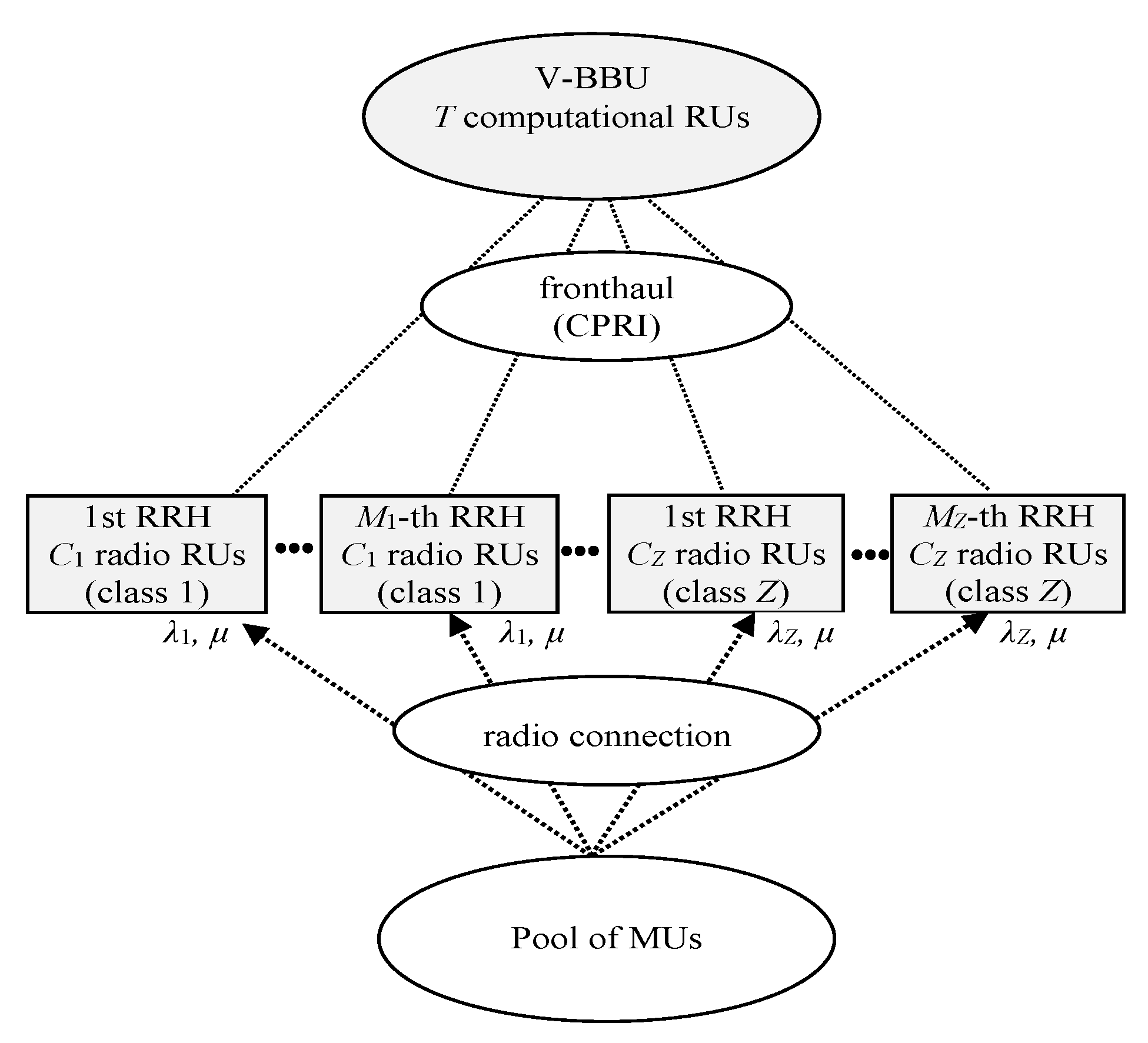
Figure 1. Multi-cluster C-RAN in the case of random traffic (SC-MC model).
Electronics 09 02120 g001
Figure 2. TC probabilities ( B 1 , m , r T C and B 1 , r ) for the first cluster and both models.
Electronics 09 02120 g002
Figure 3. TC probabilities ( B c T C and B c ) for the first cluster and both models.
Electronics 09 02120 g003
Figure 4. CC probabilities ( B 1 , m C C and B 1 C C ) for the first cluster and both models.
Electronics 09 02120 g004
Figure 5. TC probabilities ( B 2 , m , r T C and B 2 , r ) for the second cluster and both models.
Electronics 09 02120 g005
Figure 6. TC probabilities ( B c T C and B c ) for the second cluster and both models.
Electronics 09 02120 g006
Figure 7. CC probabilities ( B 2 , m C C and B 2 C C ) for the second cluster and both models.
Electronics 09 02120 g007
Publisher’s Note: MDPI stays neutral with regard to jurisdictional claims in published maps and institutional affiliations.