A Fast-Converging Scheme for the Electromagnetic Scattering from a Thin Dielectric Disk

Abstract

In this paper, the analysis of the electromagnetic scattering from a thin dielectric disk is formulated as two sets of one-dimensional integral equations in the vector Hankel transform domain by taking advantage of the revolution symmetry of the problem and by imposing the generalized boundary conditions on the disk surface. The problem is further simplified by means of Helmholtz decomposition, which allows to introduce new scalar unknows in the spectral domain. Galerkin method with complete sets of orthogonal eigenfunctions of the static parts of the integral operators, reconstructing the physical behavior of the fields, as expansion bases, is applied to discretize the integral equations. The obtained matrix equations are Fredholm second-kind equations whose coefficients are efficiently numerically evaluated by means of a suitable analytical technique. Numerical results and comparisons with the commercial software CST Microwave Studio are provided showing the accuracy and efficiency of the proposed technique.

1. Introduction

Many applications in the framework of frequency-selective surfaces, graphene structures, radome design, microstrip antennas and antenna arrays, just as examples, involve thin layers of dielectric/conducting materials [1,2,3,4,5,6,7,8,9,10]. For these reasons, such structures have been extensively studied in the past decades and even more recently. The literature devoted to this subject is principally focused on finding approximate solutions based on Rayleigh-Gans or physical optics techniques, or on proposing suitable numerical methods to achieve more accurate solutions. In the last case, when the thickness of the involved structure is much less than the free-space wavelength, the classical 3D approaches reveal to be not particularly suitable in terms of computation time, storage requirements and they can even suffer from lack of convergence.

On the other hand, the problem can be significantly simplified if the scatterer is approximated as a surface with the fields satisfying suitable boundary conditions, generally called generalized boundary conditions [11,12]. In such a case, surface integral equation formulations for the effective electric and/or magnetic current densities, taking into account the radiation conditions of the fields, are particularly attractive because the integral equations and the unknowns are defined on a finite support [12,13].

The discretization of the obtained equation is, however, a key point because the convergence of the approximate solution to the exact one cannot be generally established [14]. Moreover, it can lead to a huge ill-conditioned matrix to be numerically inverted. Sometimes, compression techniques [15,16] and/or suitable discretization schemes [17,18,19] can be usefully applied. However, a general way to overcome these problems is to recast the integral equation in hand as a Fredholm second-kind integral equation by analytically inverting a part of the operator containing the most singular one [20]. Then, due to the Fredholm’s theory, every discretization scheme preserving the Fredholm’s nature of the obtained second-kind integral equation is a convergent scheme [21].

A different approach consists in properly select the discretization scheme in order to obtain a guaranteed convergence matrix equation [20]. This means that regularization and discretization are condensed in a single step. The wide literature devoted to this subject, in the context of the analysis of propagation, radiation and scattering problems, have demonstrated that one way to reach this goal is the application of the Galerkin method with a suitable selection of the expansion functions such that the most singular part of the discretized operator is invertible with a continuous two-side inverse, and the remaining part is a compact operator [22,23,24,25,26,27,28,29,30,31,32]. Moreover, if the physical behavior of the unknowns is properly reconstructed by the expansion functions, the convergence is even fast, i.e., highly accurate results can be achieved by means of a small size coefficients’ matrix, with an obvious advantage in terms of computation time and storage requirement.

In this paper, an analytically regularizing approach for the analysis of the electromagnetic scattering from a thin dielectric disk in a homogeneous medium is presented. Two independent surface integral equations for the effective electric and magnetic currents, respectively, are obtained by imposing the generalized boundary conditions on the disk surface. Due to the revolution symmetry of the problem, all the involved functions are conveniently expanded in Fourier series and the surface integral equations are recast as sets of one-dimensional integral equations in the spectral domain for the components of each harmonic of the vector Hankel transforms (VHTs) of the effective currents. Helmholtz decomposition allows to further simplify the problem by introducing new scalar unknowns to be discretized. Galerkin method with complete sets of orthogonal eigenfunctions of the static parts of the involved integral operators, reconstructing the behavior of the unknowns at the edge and around the center of the disk, as expansion bases is used to discretize the integral equations. In this way, the Galerkin projection acts as a perfect preconditioner and the obtained matrix equations are the Fredholm second-kind matrix operator equations. Moreover, the convolution integrals are reduced to algebraic products in the spectral domain. Hence, the resulting matrix coefficients are combinations of one-dimensional improper integrals efficiently evaluated by means of a suitable analytical procedure. The presented numerical results and the comparisons with the commercial software CST Microwave Studio (CST-MWS) clearly show the accuracy and efficiency of the proposed technique.

This paper is organized as follows: Section 2 is devoted to the formulation and solution of the problem, Section 3 shows the numerical results, Section 4 is dedicated to the conclusions and an Appendix A concludes the paper.

2. Formulation and Solution of the Problem

2.1. Integral Equations in the Spectral Domain

In Figure 1, a thin dielectric disk of radius a, thickness $\tau$, dielectric permittivity $\epsilon$ and magnetic permeability $\mu$ is immersed in free space of dielectric permittivity ${\epsilon }_0$ and magnetic permeability ${\mu }_0$. A cylindrical coordinate system $\left(\rho ,\varphi ,z\right)$ with the origin at the center of the disk and the z axis orthogonal to it is introduced.

A plane wave, i.e., ${\underset{\_}{E}}^{inc}\left(\underset{\_}{r}\right)={\underset{\_}{E}}_0{e}^{-j\underset{\_}{k}\cdot \underset{\_}{r}}$ and ${\underset{\_}{H}}^{inc}\left(\underset{\_}{r}\right)=\sqrt{{\epsilon }_0/{\mu }_0}\widehat{k}\times {\underset{\_}{E}}_0{e}^{-j\underset{\_}{k}·\underset{\_}{r}}$, where $\underset{\_}{k}=-k_0\left(\sin {\theta }_0\cos {\varphi }_0\widehat{x}+\sin {\theta }_0\sin {\varphi }_0\widehat{y}+\cos {\theta }_0\widehat{z}\right)$ is the propagation vector, $k_0=2\pi /\lambda =\omega \sqrt{{\epsilon }_0{\mu }_0}$ is the free-space wavenumber, $\lambda$ is the free-space wavelength, $\omega$ is the angular frequency, $\left({\theta }_0,{\varphi }_0\right)$ identifies the propagation direction and $\underset{\_}{r}=x\widehat{x}+y\widehat{y}+z\widehat{z}$, impinges onto the disk surface generating a scattered electromagnetic field $\left({\underset{\_}{E}}^{sc}\left(\underset{\_}{r}\right),{\underset{\_}{H}}^{sc}\left(\underset{\_}{r}\right)\right)$. If $\left|\epsilon \mu \right|\gg {\epsilon }_0{\mu }_0$, $\tau \ll a$ and $\tau \ll \lambda$, the disk can be approximated as a flat zero-thickness surface, on which the following generalized boundary conditions have to be satisfied [11,12,18]:

$$\widehat{z}\times \left({\underset{\_}{E}}^{tot}\left(\rho ,\varphi ,0^{+}\right)+{\underset{\_}{E}}^{tot}\left(\rho ,\varphi ,0^{-}\right)\right)\times \widehat{z}=R_e\underset{\_}{J}\left(\rho ,\varphi \right),$$

(1a)

$$\widehat{z}\times \left({\underset{\_}{H}}^{tot}\left(\rho ,\varphi ,0^{+}\right)+{\underset{\_}{H}}^{tot}\left(\rho ,\varphi ,0^{-}\right)\right)\times \widehat{z}=R_m\underset{\_}{M}\left(\rho ,\varphi \right),$$

(1b)

for $\rho \le a$, where $\left({\underset{\_}{E}}^{tot}\left(\underset{\_}{r}\right),{\underset{\_}{H}}^{tot}\left(\underset{\_}{r}\right)\right)$ denotes the total electromagnetic field:

$$\underset{\_}{J}\left(\rho ,\varphi \right)=\widehat{z}\times \left({\underset{\_}{H}}^{sc}\left(\rho ,\varphi ,0^{+}\right)-{\underset{\_}{H}}^{sc}\left(\rho ,\varphi ,0^{-}\right)\right),$$

(2a)

$$\underset{\_}{M}\left(\rho ,\varphi \right)=-\widehat{z}\times \left({\underset{\_}{E}}^{sc}\left(\rho ,\varphi ,0^{+}\right)-{\underset{\_}{E}}^{sc}\left(\rho ,\varphi ,0^{-}\right)\right),$$

(2b)

are the effective electric and magnetic currents, respectively, and:

$$R_e=-j\sqrt{\frac{\mu }{\epsilon }}\cot \left(\frac{k_0\tau }{2}\sqrt{\frac{\epsilon \mu }{{\epsilon }_0{\mu }_0}}\right),$$

(3a)

$$R_m=-j\sqrt{\frac{\epsilon }{\mu }}\cot \left(\frac{k_0\tau }{2}\sqrt{\frac{\epsilon \mu }{{\epsilon }_0{\mu }_0}}\right),$$

(3b)

are the electric and magnetic resistivities of the disk, respectively. It is interesting to observe that the integral Equations (1a) and (1b) are decoupled for the problem in hand [11].

The uniqueness of the solution is guaranteed by requiring that the fields components satisfy, additionally, the edge conditions and the radiation conditions [20].

The revolution symmetry of the problem allows to expand all the involved functions in Fourier series. Hence, the surface integral equations for the effective electric and magnetic currents can be equivalently reduced to two infinite sets of independent one-dimensional integral equations:

$${\underset{\_}{E}}^{sc\left(n\right)}\left(\rho ,0\right)-R_e{\underset{\_}{J}}^{\left(n\right)}\left(\rho \right)=-{\underset{\_}{E}}^{inc\left(n\right)}\left(\rho ,0\right),$$

(4a)

$${\underset{\_}{H}}^{sc\left(n\right)}\left(\rho ,0\right)-R_m{\underset{\_}{M}}^{\left(n\right)}\left(\rho \right)=-{\underset{\_}{H}}^{inc\left(n\right)}\left(\rho ,0\right),$$

(4b)

for $\rho \le a$, where the apex n denotes the n-th term of the Fourier series, the symbol:

$${\underset{\_}{P}}^{\left(n\right)}(·)=\left(\begin{array}{c}{P}_{\rho }^{\left(n\right)}(·)\\ -j{P}_{\varphi }^{\left(n\right)}(·)\end{array}\right)$$

(5)

has been introduced, and the n-th harmonics of the scattered electric and magnetic fields, respectively, can be expressed in the spectral domain as follows [32]:

$${\underset{\_}{E}}^{sc\left(n\right)}\left(\rho ,0\right)={\displaystyle \underset{0}{\overset{+\infty }{\int }}{\underset{\_}{\underset{\_}{H}}}^{\left(n\right)}\left(w\rho \right){\underset{\_}{\underset{\_}{\tilde{G}}}}_e\left(w\right){\underset{\_}{\tilde{J}}}^{\left(n\right)}\left(w\right)wdw}$$

(6a)

$${\underset{\_}{H}}^{sc\left(n\right)}\left(\rho ,0\right)={\displaystyle \underset{0}{\overset{+\infty }{\int }}{\underset{\_}{\underset{\_}{H}}}^{\left(n\right)}\left(w\rho \right){\underset{\_}{\underset{\_}{\tilde{G}}}}_m\left(w\right){\underset{\_}{\tilde{M}}}^{\left(n\right)}\left(w\right)wdw}$$

(6b)

where:

$${\underset{\_}{\underset{\_}{H}}}^{\left(n\right)}\left(w\rho \right)=\left(\begin{array}{cc}{J^{\prime }}_n\left(w\rho \right)& n{J}_n\left(w\rho \right)/\left(w\rho \right)\\ n{J}_n\left(w\rho \right)/\left(w\rho \right)& {J^{\prime }}_n\left(w\rho \right)\end{array}\right),$$

(7)

$J_n(·)$ and ${J^{\prime }}_n(·)$ are the Bessel function of the first kind and order n and its first derivative with respect to the argument, respectively [33]:

$${\underset{\_}{\underset{\_}{\tilde{G}}}}_r\left(w\right)=\left(\begin{array}{cc}{\tilde{G}}_{r,C}\left(w\right)& 0\\ 0& {\tilde{G}}_{r,D}\left(w\right)\end{array}\right)=\frac{1}{2\omega {\chi }_r}\left(\begin{array}{cc}-\sqrt{k_0^2-w^2}& 0\\ 0& -k_0^2/\sqrt{k_0^2-w^2}\end{array}\right)$$

(8)

with $r\in \left\{e,m\right\}$, ${\chi }_e={\epsilon }_0$, ${\chi }_m={\mu }_0$, $\sqrt{k_0^2-w^2}=-j\sqrt{-k_0^2+w^2}$, and the following definition of the VHT of order n (VHT_n) has been introduced [34]:

$${\underset{\_}{\tilde{P}}}^{\left(n\right)}\left(w\right)={\mathrm{VHT}}_n\left({\underset{\_}{P}}^{\left(n\right)}\left(\rho \right)\right)={\displaystyle \underset{0}{\overset{+\infty }{\int }}{\underset{\_}{\underset{\_}{H}}}^{\left(n\right)}\left(w\rho \right)}{\underset{\_}{P}}^{\left(n\right)}\left(\rho \right)\rho d\rho .$$

(9)

Observing that [34]:

$${\underset{\_}{P}}^{\left(n\right)}\left(\rho \right)={\mathrm{VHT}}_n^{-1}\left({\underset{\_}{\tilde{P}}}^{\left(n\right)}\left(w\right)\right)={\displaystyle \underset{0}{\overset{+\infty }{\int }}{\underset{\_}{\underset{\_}{H}}}^{\left(n\right)}\left(w\rho \right)}{\underset{\_}{\tilde{P}}}^{\left(n\right)}\left(w\right)wdw,$$

(10)

the Equations (4) can be immediately rewritten as follows:

$${\displaystyle \underset{0}{\overset{+\infty }{\int }}{\underset{\_}{\underset{\_}{H}}}^{\left(n\right)}\left(w\rho \right)\left({\underset{\_}{\underset{\_}{\tilde{G}}}}_e\left(w\right)-R_e\underset{\_}{\underset{\_}{I}}\right){\underset{\_}{\tilde{J}}}^{\left(n\right)}\left(w\right)wdw}=-{\underset{\_}{E}}^{inc\left(n\right)}\left(\rho ,0\right),$$

(11a)

$${\displaystyle \underset{0}{\overset{+\infty }{\int }}{\underset{\_}{\underset{\_}{H}}}^{\left(n\right)}\left(w\rho \right)\left({\underset{\_}{\underset{\_}{\tilde{G}}}}_m\left(w\right)-R_m\underset{\_}{\underset{\_}{I}}\right){\underset{\_}{\tilde{M}}}^{\left(n\right)}\left(w\right)wdw}=-{\underset{\_}{H}}^{inc\left(n\right)}\left(\rho ,0\right),$$

(11b)

where $\underset{\_}{\underset{\_}{I}}$ is the identity matrix operator.

2.2. Helmholtz Decomposition

Therefore, the problem in hand has been formulated in terms of two infinite sets of one-dimensional integral equations in the spectral domain for the VHT of the harmonics of the effective currents, which are vector functions. On the other hand, the problem can be further simplified by means of the Helmholtz decomposition which leads to scalar unknowns instead of vector ones.

Let $\underset{\_}{P}\left(\rho ,\varphi \right)$ be the effective electric/magnetic current density. Due to the Helmholtz decomposition, it can be written as the superposition of a surface curl-free contribution ${\underset{\_}{P}}_C\left(\rho ,\varphi \right)={\nabla }_s{\Phi }_C\left(\rho ,\varphi \right)$ and a surface divergence-free contribution ${\underset{\_}{P}}_D\left(\rho ,\varphi \right)=\widehat{z}\times {\nabla }_s{\Phi }_D\left(\rho ,\varphi \right)$, where ${\nabla }_s=\widehat{\rho }\frac{\partial }{\partial \rho }+\widehat{\varphi }\frac{1}{\rho }\frac{\partial }{\partial \varphi }$ and ${\Phi }_T\left(\rho ,\varphi \right)$ with $T\in \left\{C,D\right\}$ are suitable potential functions [35]. Moreover, the n-th harmonic of ${\underset{\_}{P}}_T\left(\rho ,\varphi \right)$ with $T=C$ or $T=D$ can be immediately written as a function of the n-th harmonic of the corresponding potential function, i.e.,

$${\underset{\_}{P}}_C^{\left(n\right)}\left(\rho \right)=\left(\begin{array}{c}\frac{d}{d\rho }\\ \frac{n}{\rho }\end{array}\right){\Phi }_C^{\left(n\right)}\left(\rho \right),$$

(12a)

$${\underset{\_}{P}}_D^{\left(n\right)}\left(\rho \right)=-j\left(\begin{array}{c}\frac{n}{\rho }\\ \frac{d}{d\rho }\end{array}\right){\Phi }_D^{\left(n\right)}\left(\rho \right).$$

(12b)

It is possible to demonstrate (see Appendix A) that the VHT_n of the function ${\underset{\_}{P}}_T^{\left(n\right)}\left(\rho \right)$ has only one non-vanishing component, i.e.,

$${\underset{\_}{\tilde{P}}}_C^{\left(n\right)}\left(w\right)=\left(\begin{array}{c}{\tilde{P}}_C^{\left(n\right)}\left(w\right)\\ 0\end{array}\right),$$

(13a)

$${\underset{\_}{\tilde{P}}}_D^{\left(n\right)}\left(w\right)=-j\left(\begin{array}{c}0\\ {\tilde{P}}_D^{\left(n\right)}\left(w\right)\end{array}\right),$$

(13b)

where:

$${\tilde{P}}_T^{\left(n\right)}\left(w\right)={\displaystyle \underset{0}{\overset{+\infty }{\int }}{J}_n\left(w\rho \right)}{\Phi }_T^{\left(n\right)}\left(\rho \right)w\rho d\rho .$$

(14)

Henceforth, the functions (13) are assumed as new unknowns in the spectral domain.

2.3. Discretization of the Integral Equations

The obtained integral equations are discretized by means of the Galerkin method. Following the line of reasoning in [32], it is possible to show that the behavior of the n-th harmonic of the effective currents at the edge and around the center of the disk is correctly reconstructed by expanding the unknown functions ${\tilde{P}}_T^{\left(n\right)}\left(w\right)$ in complete series of weighted Bessel functions [32,36], i.e.,

$${\tilde{P}}_T^{\left(n\right)}\left(w\right)={\displaystyle \sum _{h=-1+{\delta }_{n,0}}^{+\infty }{\gamma }_{T,h}^{\left(n\right)}\sqrt{2{\eta }_{T,h}^{\left(n\right)}}\frac{J_{{\eta }_{T,h}^{\left(n\right)}}\left(aw\right)}{w^{p_T}}}.$$

(15)

where ${\delta }_{n,m}$ is the Kronecker delta, ${\gamma }_{T,h}^{\left(n\right)}$ denote the expansion coefficients, ${\eta }_{T,h}^{\left(n\right)}=\left|n\right|+2h+p{}_T+1$ and $p_C=3/2$ while $p_D=1$. Moreover, the relation ${\gamma }_{D,-1}^{\left(n\right)}=\frac{j\mathrm{sgn}\left(n\right)\left|n\right|!}{\Gamma \left(\left|n\right|+3/2\right)}\sqrt{\frac{a\left(\left|n\right|+1/2\right)}{2\left|n\right|}}{\gamma }_{C,-1}^{\left(n\right)}$ for $n\ne 0$ can be established by imposing the currents to be vanishing outside the disk surface.

Due to the spectral domain formulation, the convolution integrals are reduced to algebraic products. Hence, the coefficients of the obtained matrix equations can be readily expressed as combinations of one-dimensional integrals of the kind:

$$I_{r,T,k,h}^{\left(n\right)}=2\sqrt{{\eta }_{T,k}^{\left(n\right)}{\eta }_{T,h}^{\left(n\right)}}{\displaystyle \underset{0}{\overset{+\infty }{\int }}{\tilde{K}}_{r,T}\left(w\right)J_{{\eta }_{T,k}^{\left(n\right)}}\left(aw\right)J_{{\eta }_{T,h}^{\left(n\right)}}\left(aw\right)dw},$$

(16)

where:

$${\tilde{K}}_{r,T}\left(w\right)=\frac{{\tilde{G}}_{r,T}\left(w\right)-R_r}{w^{2p_T-1}}.$$

(17)

By extracting the asymptotic behavior of the kernel in (16), i.e., ${\tilde{K}}_{r,T}\left(w\right)\stackrel{w\to \infty }{\sim }{\tilde{K}}_{r,T}^{\infty }\left(w\right)=\frac{{\kappa }_{r,T}}{w}$, and using the well-known Weber-Schafheitlin discontinuous integral [37], the following alternative expression for the integral in (16) can be obtained:

$$I_{r,T,k,h}^{\left(n\right)}=2\sqrt{{\eta }_{T,k}^{\left(n\right)}{\eta }_{T,h}^{\left(n\right)}}{\displaystyle \underset{0}{\overset{+\infty }{\int }}\left({\tilde{K}}_{r,T}\left(w\right)-\frac{{\kappa }_{r,T}}{w}\right)J_{{\eta }_{T,k}^{\left(n\right)}}\left(aw\right)J_{{\eta }_{T,h}^{\left(n\right)}}\left(aw\right)dw}+{\kappa }_{r,T}{\delta }_{k,h}.$$

(18)

Since it is possible to demonstrate that the matrix operators associated to the first term at the right hand side of (18) are compact operators in $l^2$ [32], the obtained equations are the Fredholm second-kind matrix operator equations in $l^2$ [21], and the convergence of the discretization scheme is guaranteed.

The numerical convergence of improper integrals of oscillating functions with an algebraic decay like the one in (18) can be time-consuming when highly accurate results are searched for. This problem can be completely overcome by adopting the analytical procedure in the complex plane developed in [38], which leads to the numerical evaluation of fast converging proper integrals.

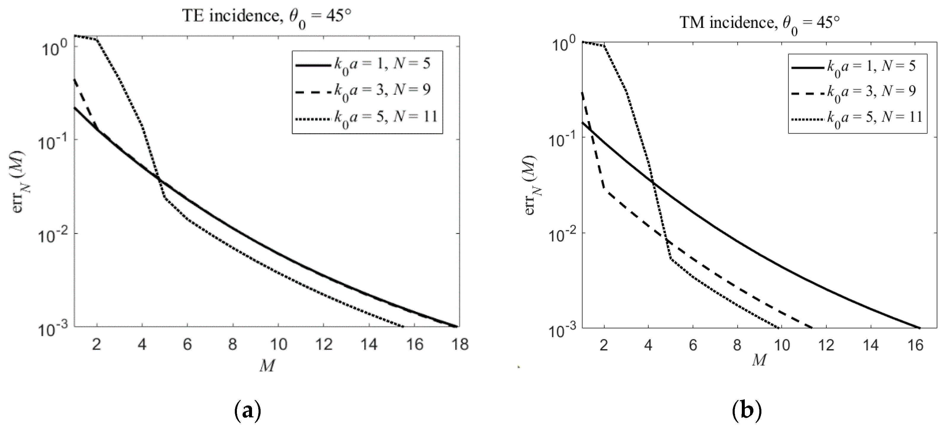
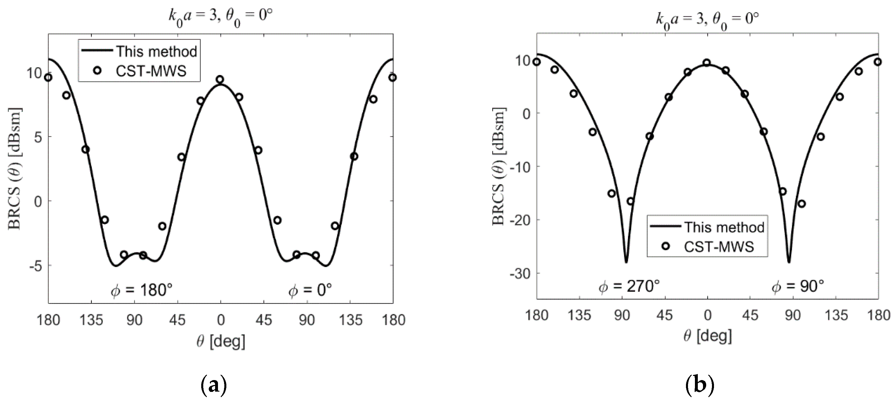
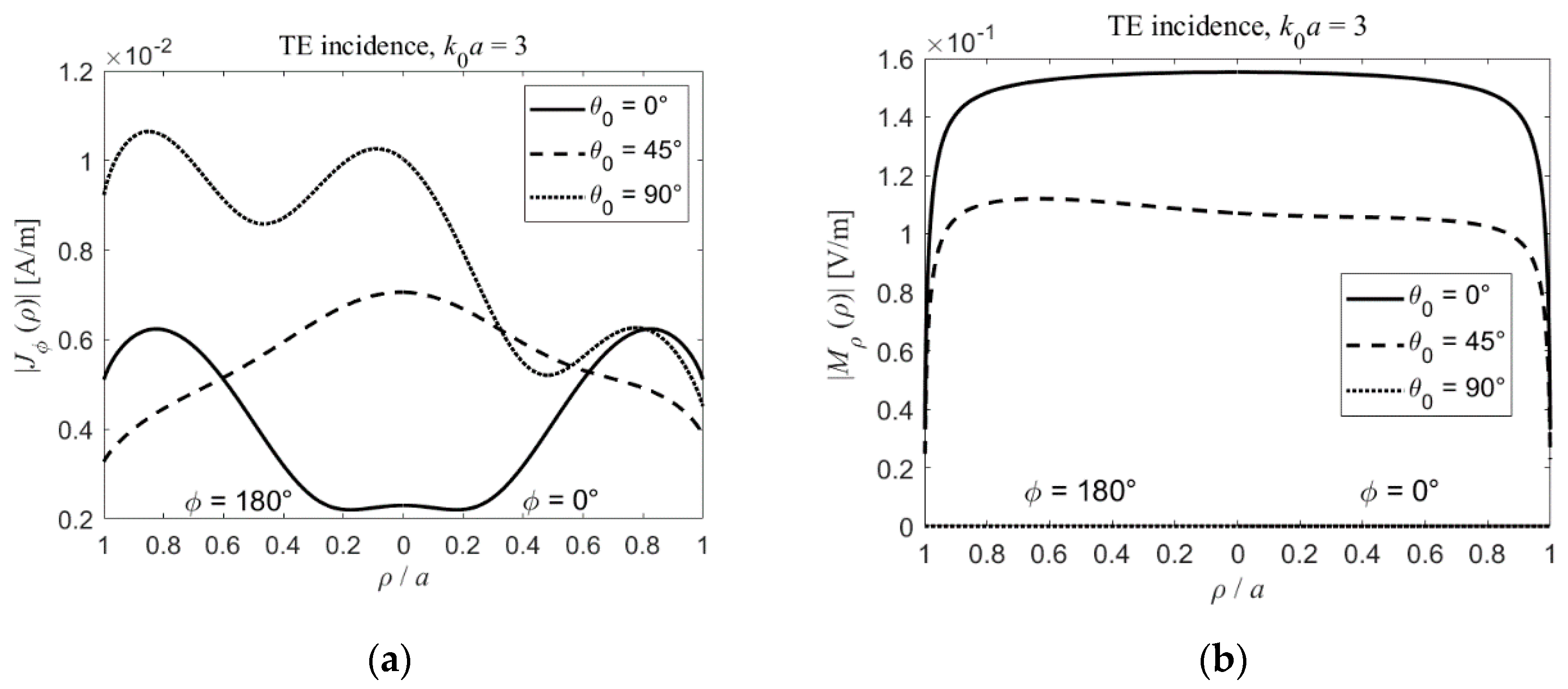
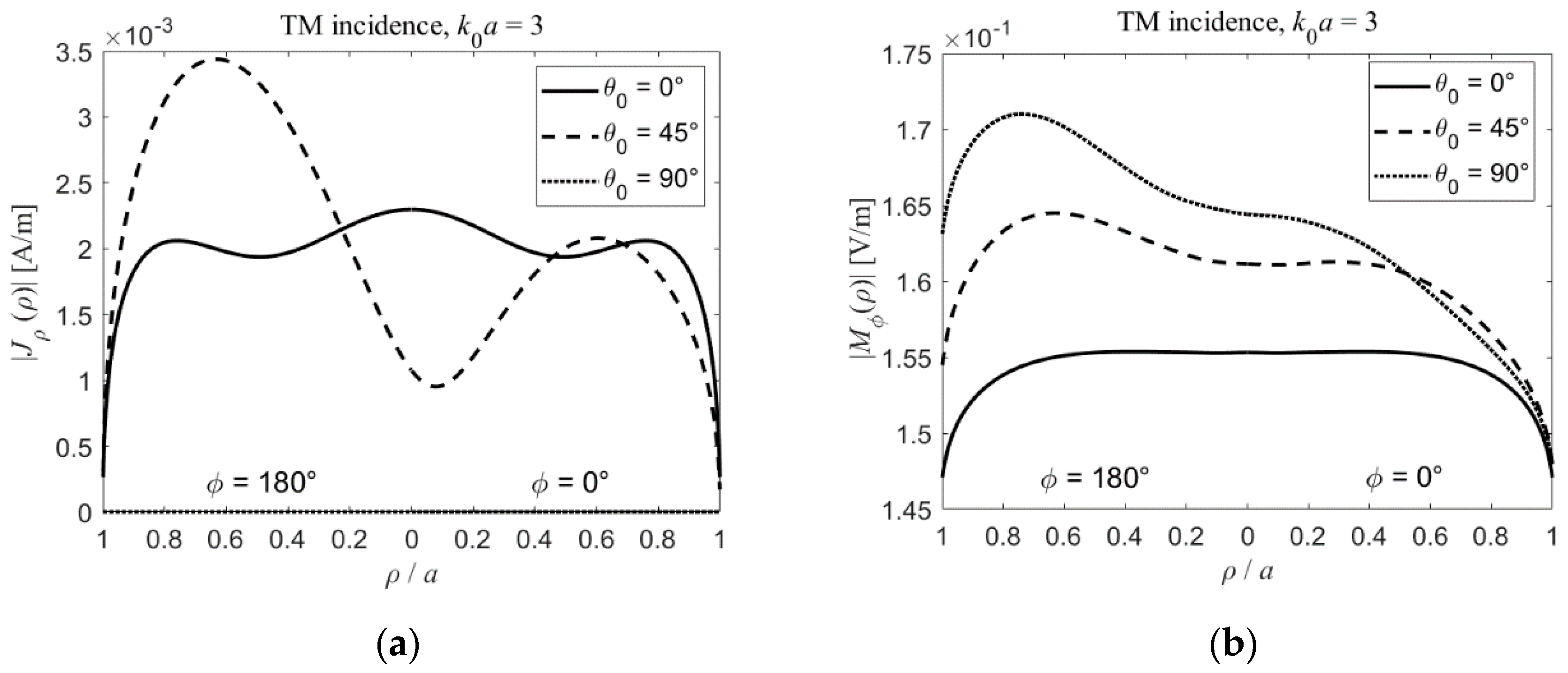
3. Results and Discussion

An approximate solution can be obtained by truncating the obtained infinite matrix equations. In order to show the fast convergence of the presented method, the following normalized truncation error is introduced:

$${\mathrm{err}}_N\left(M\right)=\sqrt{{\displaystyle \sum _{n=-N+1}^{N-1}{\Vert x_{M+1}^{\left(n\right)}-x_M^{\left(n\right)}\Vert }^2}/{\displaystyle \sum _{n=-N+1}^{N-1}{\Vert x_M^{\left(n\right)}\Vert }^2}},$$

(19)

where 2N − 1 is the number of considered harmonics estimated as in [39], $\Vert ·\Vert$ is the usual Euclidean norm and $x_M^{\left(n\right)}$ is the vector of all the expansion coefficients evaluated by using M expansion functions for each unknown. All the simulations are performed on a laptop equipped with an Intel Core i7-8550u 1.8 GHz CPU and 16 GB RAM, running Windows 10 and the integrals of the coefficients’ matrix evaluated by means of an adaptive Gauss-Legendre quadrature routine implemented in the Matlab environment.

In Figure 2, the normalized truncation error, when a plane wave with incidence direction ${\theta }_0=45°$, ${\varphi }_0=0°$, electric field amplitude $\left|{\underset{\_}{E}}_0\right|=1 \mathrm{V}/\mathrm{m}$, TE incidence and TM incidence impinges onto a disk with a normalized radius $k_{0}a=1,3,5$, thickness τ = 0.05a, dielectric permittivity $\epsilon =\left(10.5-j0.3\right){\epsilon }_0$ and magnetic permeability $\mu ={\mu }_0$, is plotted as a function of M for $N=5,9,11$, respectively.

As can be seen in Figure 2, the convergence is very fast in all the examined cases. Indeed, in the worst case, an error less than ${10}^{-2}$ is achieved form M = 10, while M = 18 allows to obtain an error less than ${10}^{-3}$. Moreover, an increased normalized radius leads only to a greater number of harmonics to be used. This is because the values of the electric and magnetic resistivities are functions of the normalized thickness ($k_0\tau$) and, therefore, a change in the normalized radius can increase or decrease the rate of convergence. In Figure 3, the normalized truncation error is plotted as a function of M for three incidence directions, i.e., for ${\theta }_0=0°,45°,90°$ and ${\varphi }_0=0°$, and for $\left|{\underset{\_}{E}}_0\right|=1 \mathrm{V}/\mathrm{m}$, TE incidence and TM incidence, $N=2,9,11$, $k_{0}a=3$, $\epsilon =\left(10.5-j0.3\right){\epsilon }_0$, $\mu ={\mu }_0$. As expected, a change in the incident angle ${\theta }_0$ affects the number of harmonics to be used in order to achieve a given accuracy. On the other hand, for TE incidence, the change of ${\theta }_0$ does not significantly affect the number of expansion functions to be used while, for TM incidence, the convergence is even faster if ${\theta }_0$ is larger. To conclude, it is worth noting that a normalized truncation error less than ${10}^{-3}$ can be achieved in the worst of the cases examined in this paper by filling a coefficient matrix of about 50,000 elements, with a computation time less than 2 min.

As clearly stated before, the convergence of the proposed method is guaranteed. Hence, comparisons with CST-MWS are just provided in order to validate the numerical implementation and to show the accuracy and the efficiency of the proposed approach.

In Figure 4 the Bistatic Radar Cross Section (BRCS) for a disk with $k_{0}a=3$, τ = 0.05a, $\epsilon =\left(10.5-j0.3\right){\epsilon }_0$ and $\mu ={\mu }_0$, on which a plane wave orthogonally impinges with ${\underset{\_}{E}}_0=E_0\widehat{y}$, obtained for M = 19 and N = 2 in order to achieve a normalized truncation error less than ${10}^{-3}$, is plotted and compared with the results provided by CST-MWS. The agreement is quite good. It is interesting to note, however, that CST-MWS requires a computation time of 80 min and 9.4 M mesh-cells to reconstruct the plotted solution. After all, to the best of the authors knowledge, CST-MWS does not provide a 2D model for dielectric objects and an accurate simulation of the considered 3D object has turned out to be time-consuming and particularly burdensome in terms of memory requirement. As a result, the proposed approach drastically outperforms CST-MWS in terms of both computation time and storage requirements.

The proposed method allows the simple reconstruction of near field and far field parameters. For the sake of completeness, in Figure 5, Figure 6 and Figure 7, the effective electric and magnetic currents and the BRCSs for a disk with $k_{0}a=3$, τ = 0.05a, $\epsilon =\left(10.5-j0.3\right){\epsilon }_0$ and $\mu ={\mu }_0$, when a plane wave with $\left|{\underset{\_}{E}}_0\right|=1 \mathrm{V}/\mathrm{m}$, TE incidence and TM incidence, and three incidence directions, i.e., ${\theta }_0=0°,45°,90°$ and ${\varphi }_0=0°$, impinges onto the disk surface, are shown.

In Figure 5, where the TE incidence is considered, the absolute values of the non-vanishing components of the effective electric and magnetic currents along the x axis ($\varphi =0°,180°$), i.e., the azimuthal component of the effective electric current and the radial component of the effective magnetic current, are plotted as functions of $\rho /a$. Similarly, in Figure 6, the absolute values of the non-vanishing components of the effective currents along the x axis obtained for TM incidence, i.e., the radial component of the effective electric current and the azimuthal component of the effective magnetic current, are plotted as a function of $\rho /a$. As expected, the radial component of the effective magnetic current for TE incidence and the radial component of the effective electric current for TM incidence vanish at grazing incidence (${\theta }_0=90°$) due to the symmetry of the problem with respect to the z axis. To conclude, in Figure 7, the BRCSs for both TM incidence and TE incidence are plotted in the plane $\varphi =0°,180°$ as a function of the observation angle $\theta$ and compared with quite good agreement with the results provided by CST-MWS by means of the same discretization parameters used to reconstruct the behavior in Figure 3. It is worth noting that the low number of expansion functions and harmonics used to reconstruct the currents and the BRCSs with the proposed approach, i.e., M = 19 and N = 11, is, however, enough to guarantee a normalized truncation error less than 10⁻³.

4. Conclusions

In this paper, a new analytically regularizing scheme for the analysis of the electromagnetic scattering from a thin dielectric disk has been presented. The method is accurate and efficient, leads to a quick evaluation of near-field and far-field parameters and drastically outperforms the general-purpose commercial software CST-MWS. Future perspectives are the generalization of the presented method to the analysis of arrays of disks and disks in layered media.

References

1. LeVine, D.M.; Schneider, A.; Lang, R.H.; Carter, H.G. Scattering from thin dielectric disks. IEEE Trans. Antennas Propag. 1985, 33, 1410–1413. [Google Scholar] [CrossRef] [Green Version]
2. Karam, M.A.; Fung, A.K.; Antar, Y.M. Electromagnetic wave scattering from some vegetation samples. IEEE Trans. Geosci. Remote Sens. 1988, 26, 799–808. [Google Scholar] [CrossRef] [Green Version]
3. Yang, F.; Rahmat-Samii, Y. Microstrip antennas integrated with electromagnetic band-gap (EBG) structures: A low mutual coupling design for array applications. IEEE Trans. Antennas Propag. 2003, 51, 2936–2946. [Google Scholar] [CrossRef] [Green Version]
4. Pan, G.; Narayanan, R.M. Electromagnetic scattering from dielectric sheet using the method of moments with approximate boundary condition. Electromagnetics 2004, 24, 369–384. [Google Scholar] [CrossRef]
5. Koh, I.S.; Sarabandi, K. A new approximate solution for scattering by thin dielectric disks of arbitrary size and shape. IEEE Trans. Antennas Propag. 2005, 53, 1920–1926. [Google Scholar] [CrossRef] [Green Version]
6. Raffaelli, S.; Sipus, Z.; Kildal, P.-S. Analysis and measurements of conformal patch array antennas on multilayer circular cylinder. IEEE Trans. Antennas Propag. 2005, 53, 1105–1113. [Google Scholar] [CrossRef]
7. Schild, S.; Chavannes, N.; Kuster, N. A robust method to accurately treat arbitrarily curved 3-D thin conductive sheets in FDTD. IEEE Trans. Antennas Propag. 2007, 55, 3587–3594. [Google Scholar] [CrossRef]
8. Balaban, M.V.; Sauleau, R.; Benson, T.M.; Nosich, A.I. Accurate quantification of the Purcell effect in the presence of a microdisk of nanoscale thickness. IET Micro Nano Lett. 2011, 6, 393–396. [Google Scholar] [CrossRef]
9. Lee, J.; Yoo, M.; Lim, S. A study of ultra-thin single layer frequency selective surface microwave absorbers with three different bandwidths using double resonance. IEEE Trans. Antennas Propag. 2015, 63, 221–230. [Google Scholar] [CrossRef]
10. Omar, A.A.; Shen, Z. Thin 3-D bandpass frequency-selective structure based on folded substrate for conformal radome applications. IEEE Trans. Antennas Propag. 2019, 67, 282–290. [Google Scholar] [CrossRef]
11. Bleszynski, E.; Bleszynski, M.; Jaroszewicz, T. Surface-integral equations for electrmagnetic scattering from impenetrable and penetrable sheets. IEEE Antennas Propagat. Magaz. 1993, 35, 14–24. [Google Scholar] [CrossRef]
12. Balaban, M.V.; Sauleau, R.; Benson, T.M.; Nosich, A.I. Dual integral equations technique in electromagnetic scattering by a thin disk. Prog. Electromagn. Res. B 2009, 16, 107–126. [Google Scholar] [CrossRef] [Green Version]
13. Nazarchuk, Z.; Kobayashi, K. Mathematical modelling of electromagnetic scattering from a thin penetrable target. Prog. Electromagn. Res. 2005, 55, 95–116. [Google Scholar] [CrossRef] [Green Version]
14. Dudley, D.G. Error minimization and convergence in numerical methods. Electromagnetics 1985, 5, 89–97. [Google Scholar] [CrossRef]
15. Migliore, M.D.; Pinchera, D.; Lucido, M.; Schettino, F.; Panariello, G. A sparse recovery approach for pattern correction of active arrays in presence of element failures. IEEE Antennas Wirel. Propag. Lett. 2015, 14, 1027–1030. [Google Scholar] [CrossRef]
16. Pinchera, D.; Migliore, M.D.; Lucido, M.; Schettino, F.; Panariello, G. A compressive-sensing inspired alternate projection algorithm for sparse array synthesis. Electronics 2017, 6, 3. [Google Scholar] [CrossRef] [Green Version]
17. Bulygin, V.S.; Gandel, Y.V.; Nosich, A.I. Nystrom-type method in three-dimensional electromagnetic diffraction by a finite PEC rotationally symmetric surface. IEEE Trans. Antennas Propag. 2012, 60, 4710–4718. [Google Scholar] [CrossRef]
18. Sukharevsky, I.O.; Shapoval, O.V.; Nosich, A.I.; Altintas, A. Validity and limitations of the median-line integral equation technique in the scattering by material strips of sub-wavelength thickness. IEEE Trans. Antennas Propag. 2014, 62, 3623–3631. [Google Scholar] [CrossRef]
19. Tsalamengas, J.L. Quadrature rules for weakly singular, strongly singular, and hypersingular integrals in boundary integral equation methods. J. Computat. Phys. 2015, 303, 498–513. [Google Scholar] [CrossRef]
20. Nosich, A.I. Method of analytical regularization in computational photonics. Radio Sci. 2016, 51, 1421–1430. [Google Scholar] [CrossRef]
21. Kantorovich, L.V.; Akilov, G.P. Functional Analysis, 2nd ed.; Pergamon Press: Oxford, UK, 2014. [Google Scholar]
22. Veliev, E.I.; Veremey, V.V. Numerical-analytical approach for the solution to the wave scattering by polygonal cylinders and flat strip structures. In Analytical and Numerical Methods in Electromagnetic Wave Theory; Hashimoto, M., Idemen, M., Tretyakov, O.A., Eds.; Science House: Tokyo, Japan, 1993. [Google Scholar]
23. Bliznyuk, N.Y.; Nosich, A.I.; Khizhnyak, A.N. Accurate computation of a circular-disk printed antenna axisymmetrically excited by an electric dipole. Microw. Opt. Technol. Lett. 2000, 25, 211–216. [Google Scholar] [CrossRef]
24. Losada, V.; Boix, R.R.; Medina, F. Fast and accurate algorithm for the short-pulse electromagnetic scattering from conducting circular plates buried inside a lossy dispersive halfspace. IEEE Trans. Geosci. Remote Sens. 2003, 41, 988–997. [Google Scholar] [CrossRef]
25. Hongo, K.; Naqvi, Q.A. Diffraction of electromagnetic wave by disk and circular hole in a perfectly conducting plane. Prog. Electromagn. Res. 2007, 68, 113–150. [Google Scholar] [CrossRef] [Green Version]
26. Lucido, M.; Panariello, G.; Schettino, F. TE scattering by arbitrarily connected conducting strips. IEEE Trans. Antennas Propag. 2009, 57, 2212–2216. [Google Scholar] [CrossRef]
27. Coluccini, G.; Lucido, M.; Panariello, G. TM scattering by perfectly conducting polygonal cross-section cylinders: A new surface current density expansion retaining up to the second-order edge behavior. IEEE Trans. Antennas Propag. 2012, 60, 407–412. [Google Scholar] [CrossRef]
28. Coluccini, G.; Lucido, M.; Panariello, G. Spectral domain analysis of open single and coupled microstrip lines with polygonal cross-section in bound and leaky regimes. IEEE Trans. Microw. Theory Technol. 2013, 61, 736–745. [Google Scholar] [CrossRef]
29. Coluccini, G.; Lucido, M. A new high efficient analysis of the scattering by a perfectly conducting rectangular plate. IEEE Trans. Antennas Propag. 2013, 61, 2615–2622. [Google Scholar] [CrossRef]
30. Lucido, M. Electromagnetic scattering by a perfectly conducting rectangular plate buried in a lossy half-space. IEEE Trans. Geosci. Remote Sens. 2014, 52, 6368–6378. [Google Scholar] [CrossRef]
31. Lucido, M.; Migliore, M.D.; Pinchera, D. A new analytically regularizing method for the analysis of the scattering by a hollow finite-length PEC circular cylinder. Prog. Electromagn. Res. B 2016, 70, 55–71. [Google Scholar] [CrossRef] [Green Version]
32. Lucido, M.; Panariello, G.; Schettino, F. Scattering by a zero-thickness PEC disk: A new analytically regularizing procedure based on Helmholtz decomposition and Galerkin method. Radio Sci. 2017, 52, 2–14. [Google Scholar] [CrossRef]
33. Abramowitz, M.; Stegun, I.A. Handbook of Mathematical Functions; Verlag Harri Deutsch: Frankfurt, Germany, 1984. [Google Scholar]
34. Chew, W.C.; Kong, J.A. Resonance of nonaxial symmetric modes in circular microstrip disk antenna. J. Math. Phys. 1980, 21, 2590–2598. [Google Scholar] [CrossRef]
35. Van Bladel, J. A discussion of Helmholtz’ theorem on a surface. AEÜ 1993, 47, 131–136. [Google Scholar]
36. Wilkins, J.E. Neumann series of Bessel functions. Trans. Am. Math. Soc. 1948, 64, 359–385. [Google Scholar] [CrossRef]
37. Gradstein, S.; Ryzhik, I.M. Tables of Integrals, Series and Products; Academic Press: New York, NY, USA, 2000. [Google Scholar]
38. Lucido, M.; Di Murro, F.; Panariello, G. Electromagnetic scattering from a zero-thickness PEC disk: A note on the Helmholtz-Galerkin analytically regularizing procedure. Prog. Electromagn. Res. Lett. 2017, 71, 7–13. [Google Scholar]
39. Geng, N.; Carin, L. Wide-band electromagnetic scattering from a dielectric BOR buried in a layered lossy dispersive medium. IEEE Trans. Antennas Propag. 1999, 47, 610–619. [Google Scholar] [CrossRef]
Figure 1. Geometry of the problem: (a) a thin dielectric disk, of radius a, thickness τ , dielectric permittivity ε and magnetic permeability μ , immersed in free space of dielectric permittivity ε 0 and magnetic permeability μ 0 ; (b) a plane wave impinging onto the disk surface with propagation direction ( θ 0 , ϕ 0 ) .
Electronics 09 01451 g001
Figure 2. Normalized truncation error for disks with different radii ( k 0 a = 1 , 3 , 5 ). N = 5 , 9 , 11 , τ = 0.05a, ε = ( 10.5 j 0.3 ) ε 0 , μ = μ 0 , θ 0 = 45 ° , ϕ 0 = 0 ° , | E _ 0 | = 1   V / m , (a) TE incidence and (b) TM incidence.
Electronics 09 01451 g002
Figure 3. Normalized truncation error for a disk for three incidence directions ( θ 0 = 0 ° , 45 ° , 90 ° and ϕ 0 = 0 ° ). N = 2 , 9 , 11 , k 0 a = 3 , τ = 0.05a, ε = ( 10.5 j 0.3 ) ε 0 , μ = μ 0 . | E _ 0 | = 1   V / m , (a) TE incidence and (b) TM incidence.
Electronics 09 01451 g003
Figure 4. BRCS (a) along the x axis and (b) along the y axis, for a disk with k 0 a = 3 , τ = 0.05a, ε = ( 10.5 j 0.3 ) ε 0 , μ = μ 0 . θ 0 = 0 ° , E _ 0 = E 0 y ^ . Lines: this method; symbols: data from CST-MWS.
Electronics 09 01451 g004
Figure 5. Effective (a) electric and (b) magnetic currents on a disk along the x axis for three incidence directions ( θ 0 = 0 ° , 45 ° , 90 ° and ϕ 0 = 0 ° ). k 0 a = 3 , τ = 0.05a, ε = ( 10.5 j 0.3 ) ε 0 , μ = μ 0 . | E _ 0 | = 1   V / m and TE incidence.
Electronics 09 01451 g005
Figure 6. Effective (a) electric and (b) magnetic currents on a disk along the x axis for three incidence directions ( θ 0 = 0 ° , 45 ° , 90 ° and ϕ 0 = 0 ° ). k 0 a = 3 , τ = 0.05a, ε = ( 10.5 j 0.3 ) ε 0 , μ = μ 0 . | E _ 0 | = 1   V / m and TM incidence.
Electronics 09 01451 g006
Figure 7. BRCS for a disk in the plane ϕ = 0 ° ,   180 ° for three incidence directions ( θ 0 = 0 ° , 45 ° , 90 ° and ϕ 0 = 0 ° ). k 0 a = 3 , τ = 0.05a, ε = ( 10.5 j 0.3 ) ε 0 , μ = μ 0 . (a) TE incidence and (b) TM incidence. Lines: this method; symbols: data from CST-MWS.
Electronics 09 01451 g007