2. Mathematical Formulation
To compare electrical AC and DC distribution to provide electrical service in rural areas we assume that all the power consumptions have unity power factor and the voltage profile for both technologies is the same. The main characteristic of the proposed formulation is that the distribution network lacks of a voltage controlled node, since the operation is governed by the best coordination between renewable, batteries, and fossil fuels that guarantees the power supply to all the loads during a daily operative scenario. Regarding possible objective function in rural isolated areas two operative scenarios are considered: (i) minimization of the total grid energy losses, and (ii) minimization of the greenhouse emissions by diesel generators. Both objective functions are formulated under an optimal power flow environment.
In the case of the mathematical model of the battery energy storage systems we assume a linear representation to facilitate the implementation in GAMS environment based on the simplified model proposed in [
34] which considers that in the conversion stage all the energy losses are neglected, i.e., 100% of efficiency in all the power electronic interface [
7,
14]; nevertheless, if more accurate battery models are required, then, references [
35,
36] can be consulted.
2.1. Optimal Power Flow Model in AC Grids
The Optimal power flow (OPF) problem in AC networks is a classical non-linear non-convex optimization problem due to the presence of the active and reactive power balance equations. Here, we consider OPF formulation presented in [
7] to analyze distribution networks without constant voltage suppliers. The complete formulation of the OPF problem for AC grids is presented below:
Objective Functions
where
and
are the objective function values related to the amount of greenhouse emissions and energy losses per day, respectively.
represents the quantity of CO
emitted to the atmosphere in
by a diesel generator connected at node
i,
is the active power delivered by the diesel generator connected at node
i in the period of time
t;
is the length of the period of time considered (typically 1 h).
is the value of the admittance that relates nodes
i and
j, which have voltages
and
at each period of time
t.
is the angle of the voltage at node
i in the interval of time
t, and
is the angle of the admittance between nodes
i and
j. Please note that
and
are the sets that contains all the nodes in the grid and the total of periods of time of the operation horizon.
Set of Constraints
The power balance equations in the AC power flow are related to the amount of active and reactive power injected at each node
i in each period of time
t. These take the following form:
where
and
are the active and reactive power generation by renewable sources connected at node
i in the period of time
t;
and
are the active and reactive power capabilities in batteries and
and
represent the active and reactive power demands, respectively. Please note that in the literature it is recommended that batteries can operate with unity power factor which implies that
[
14,
37].
Constraints related with batteries are listed below:
where
is the state-of-charge of the battery
b connected at node
i in the period of time
t, which is bounded by
and
; note that the state-of-charge can be interpreted as the quantity of energy stored in the battery in percentage.
is the charging/discharging coefficient of the battery
b.
and
represent the minimum and maximum power allowable draws/injections at node
i for secure operation of the battery at each period of time.
and
represent the initial and final state-of-charges defined by the utility to operate the battery, i.e., the initial condition of the economic dispatch problem at
and the final operative consign at the end of the operation period
.
The complete interpretation of the mathematical models (
1)–(
3) is as follows: Expression (
1a) determines the value of the objective function regarding greenhouse gas emissions to the atmosphere by diesel generation. Equation (
1b) defines the total energy losses in all the conductors of the network during the operation horizon (i.e., typically 24 h). Expressions (
2a) and (
2b) define the power balance constraints regarding active and reactive components of the power at each node. Equation (
3a) calculates future the state-of-charge in the battery for each period of time as function of the current charge and the power injection/absorption to/from the grid. Expressions (
3b) and (
3c) determine the maximum and minimum values allowed to the state-of-charge (energy stored) in the battery as well as its maximum power injection (discharging state) or absorption (charging state), respectively. Finally, Equations (
3d) and (
3e) determine the initial state-of-charge of the battery and the final operative consign defined by the utility. These are defined as function of the operational requirements of the network. Nevertheless, in specialized literature it is recommended for Ion-Lithium batteries to start and end the day with
of state of charge [
14].
Remark 1. The mathematical model for the optimal operation of AC networks with renewables and batteries defined from (1) to (3) is non-linear and non-convex due to the power balance constraints which makes difficult to reach the global optimum [8]. For this reason, here we recurred to the GAMS optimization software to solve this problem to make our results comparable to those obtained from the mathematical model regarding DC grids reported in next subsection. Remark 2. The studied optimization model (1)–(3) corresponds to a single-phase representation of AC distribution network that can be used if: (i) the AC network is indeed a single-phase network which is the most typical scenario in low-voltage distribution environments, or (ii) it is a three-phase balanced distribution network that can be represented through a single-phase equivalent model [7]. 2.2. Optimal Power Flow Model in DC Grids
The mathematical formulation of the optimal power flow problem for DC networks can be obtained directly from the AC formulation by simplifying the objective function regarding energy losses minimization. Also, power balance constraints can be simplified as follows:
- ✓
The angle of the voltage do not exist () in DC networks since no frequency concept is present in these networks.
- ✓
The reactive power constraint disappears in the DC paradigm, since it is a concept regarding inductors and capacitors in AC grids, and in DC grids they behave as short- and open-circuits, respectively.
- ✓
The admittance matrix in DC grids is only defined by real numbers () regarding only with resistive effects in branches and loads, i.e., .
With these assumptions, the objective function of the DC optimal power flow and the power balance constraint takes the following forms:
Objective Function Regarding Energy Losses
where
is the amount of energy losses in all the branches of the DC network.
Power Balance Constraint
Remark 3. The complete mathematical model of the optimal power flow problem in DC grids is composed by the greenhouse gas emission objective function (1a), the objective function regarding energy losses minimization defined by (4), the power balance constraint (5) and the remainder of constraints defined in (3). It is worthy to mention that the model of the optimal power flow in DC grids is also non-linear and non-convex due to the product between voltage variables in the power balance constraint, which makes necessary to use specialized software (i.e., GAMS) to solve it efficiently [
16].
3. Solution Methodology
To solve the optimal power flow problems in AC and DC grids in this paper it is selected the GAMS software to implement their mathematical structures with a non-linear programming (NLP) solver that typically works with interior point methods to reach the optimal solution [
36,
38].
GAMS software has been largely used in specialized literature to address non-linear non-convex optimization problems in many areas of engineering, some of these works are: optimal planning and operation of power systems with batteries in AC and DC networks [
36,
37,
39,
40]; optimal location of distributed generators [
13,
22,
41,
42]; optimal design of osmotic power plants [
43]; optimal design of water distribution networks [
44]; stability analysis in DC networks [
45]; optimal design of thermoacoustic engines [
46]; optimal location of protective devices [
47], and optimal planning of distribution networks [
30], among others.
In general terms, GAMS software is a powerful optimization package that solves complex optimization problems focused on the mathematical formulation of the problem rather than the solution methodology [
38]. This represents an ideal situation to introduce students and researchers with mathematical optimization [
36]. The main characteristics of the GAMS software can be summarized as follows:
- ✓
It works with a compact model, i.e., by using the symbolic representation of the problem such as reported in model (
1)–(
3).
- ✓
The parametric information of the mathematical model is introduced via constants, vectors and matrices, which are named in GAMS as scalars, parameters and tables.
- ✓
Multiple optimization models can be selected depending on the nature of the problem under study. These models can be linear programming, non-linear programming, or mixed-integer combinations.
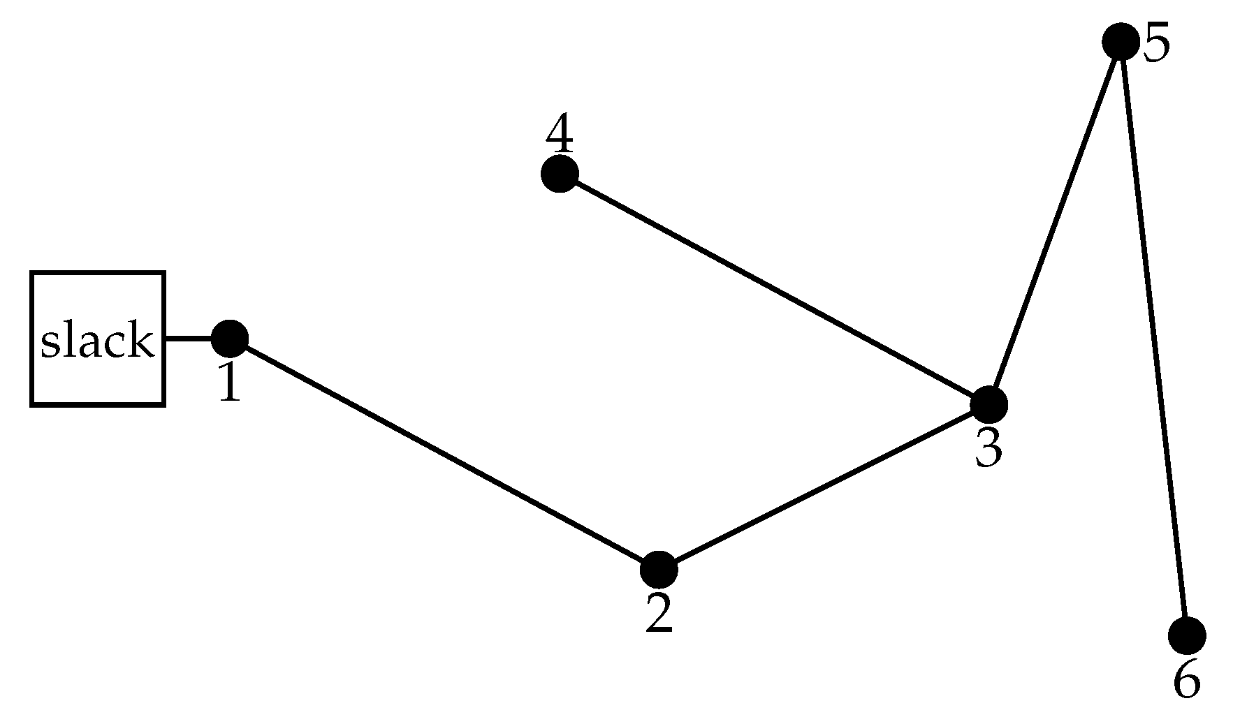
A numerical example is presented to understand the use of GAMS software to solve optimization problems with non-linear and non-convex structure. To do so, below it is presented the solution of the power flow problem for a small test feeder that can be operated with AC or DC technology. In the case of the AC technology, it is important to mention that this grid corresponds to a low-voltage distribution network with a single-phase structure, which is the most typical operation case in low-voltage applications [
48]. The configuration of this test feeder is presented in
Figure 1. This test feeder is composed by six nodes and five distribution lines (radial topology). The information of the branches and loads is reported in
Table 1. Please note that to make both configurations comparable, we assume unity power factor in all the loads. In addition, this system operates with
V typically found in Colombian AC grids.
Please note that this example is a typical low-voltage distribution network where distribution transformers have nominal power of 75 kVA. The implementation of the optimal power flow problem for this test system considers:
- ✓
A unique hour of analysis.
- ✓
Operation with unity power factor in all the loads.
- ✓
No presence of distributed generators or batteries.
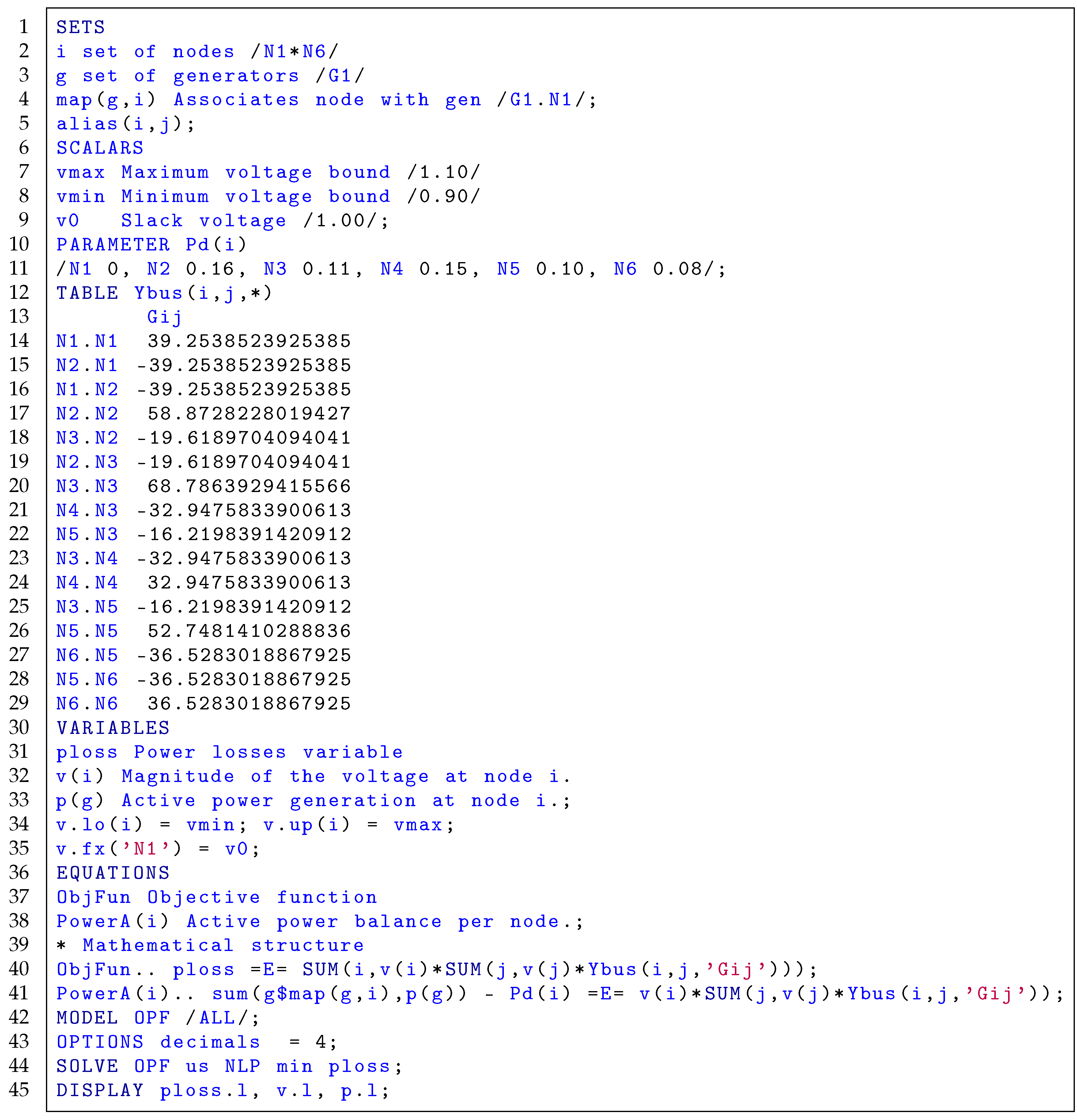
The simplified mathematical model for the optimal power flow in AC grids is presented below:
The implementation of the simplified mathematical model (
6) for the optimal power flow analysis in AC grids is presented in Listing 1.
In the case of the DC model the set of equations reported in (
6) can be simplified as presented in Equation (
7)
The implementation of this simplified mathematical model (
6) for the optimal power flow analysis in DC grids is presented in Listing 2.
Once both models (i.e., Equations (
6) and (
7)) are solved using the CONOPT solver in GAMS by using algorithms presented in Listings 1 and 2, we reach the solution of the voltage profiles reported in
Table 2. Please note that for both cases the lowest voltage occurs at node 6 being
V for the AC grid and
V for the DC network. These results imply a difference of about
V between both networks.
Additionally, power losses in the AC grid are kW, and kW in the DC case (i.e., a difference about 10 W). These results demonstrate that even considering unity power factor at all the loads, the distribution using DC technology is more efficient than the AC counterpart. The voltage drop in lines is lower due to the irrelevance of inductive reactance of the lines.
An important fact when comparing AC and DC configurations is the amount of reactive power required by the AC grid to operate adequately. In this sense, in this small example the grid needs to generate about
kVAr, which corresponds to reactive power losses through all the lines. This obviously does not occurs in the DC paradigm since reactive effect is not presented as previously mentioned. An additional simulation case in this small test feeder is made in the case of the AC distribution network by considering that all the loads are operated with a lagging power factor of 0.95. In these conditions, the total grid losses exhibit by this network are about
kW and the minimum voltage profile is about 221.04 V at node 6. These results imply that in comparison to the unity power factor operation case, the reactive power consumption at all the loads makes that the power losses to be increased about 0.37 kW, requiring at the substation node 23.40 kVAr to supply the reactive power requirements at all the loads; and that the voltage at the node has worsened about 5.76 V. Please note that when reactive power is considered for loads in the AC grid, its behavior affects and worsens the results of the comparison with respect to the unity Please note that these results are particularly important when voltage increase to medium level, since these differences become in tens of volts and hundreds of watts. In
Section 6 these impacts will be widely discussed under an economic dispatch environment in the 33-node test feeder taking into account higher penetration of renewables and battery energy storage systems.
| Listing 1. Algorithm implemented in GAMS for OPF model (6). |
![Electronics 09 01352 i001]() |
| Listing 2. Algorithm implemented in GAMS for the OPF model (7). |
![Electronics 09 01352 i002]() |
It is worth mentioning that as described in
Section 5, the comparisons made in this research regarding the efficiency comparison between AC and DC paradigms are focused on the distribution stage, which implies that we will not consider power losses in the power electronic interfaces used for interfacing renewable sources and battery energy storage systems. Nevertheless, these will be able to be explored in future research regarding energy distribution technologies and power electronic interfaces for batteries and renewables.
Remark 4. Regarding optimal implementation in GAMS environment of the OPF problem for AC and DC grids depicted in Listings 1 and 2, we can observe that the DC model is pretty simple with less variables (no angles), which makes this easiest to be solved since its nonlinearities are soft when compared to the AC model that contains trigonometric functions.
4. Generation Reactive Power in DC Grids with Voltage Source Converter Interfaces
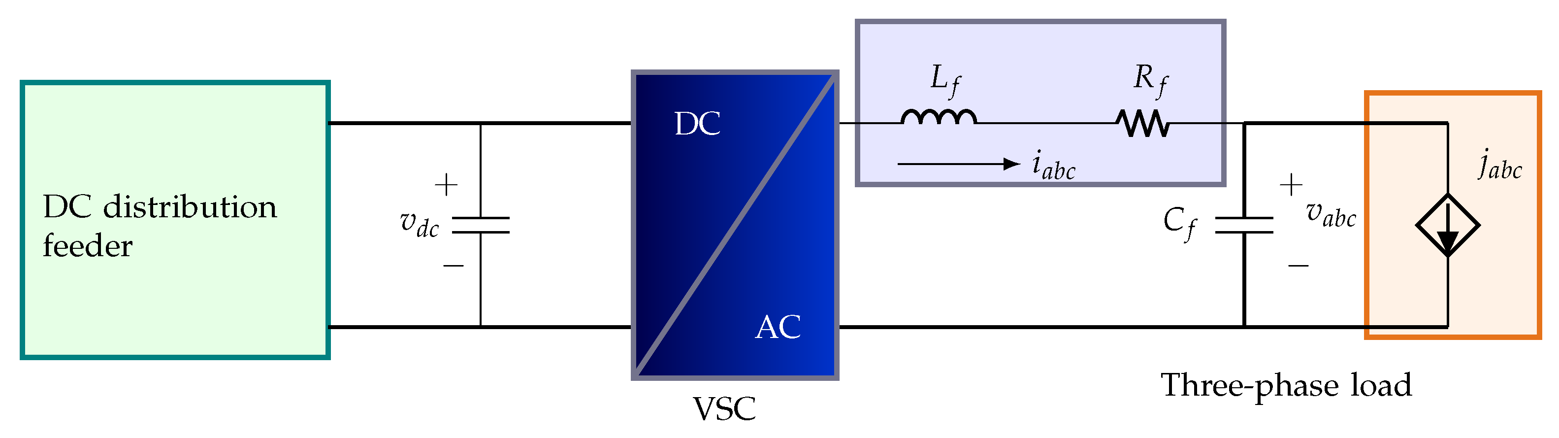
To provide apparent power to three-phase loads in medium- and low-voltage levels using DC distribution feeders, it is required a power electronic interface, i.e., voltage source converter (VSC) (A voltage source converter interface corresponds to a power electronic converter that is fed by a DC source that provides the required active power in the AC side, which is managed by controlling the switches (on or off) states via pulse-width modulation techniques to provide a sinusoidal voltage signal to AC loads [
3,
32]) that manages the active power interchange between the DC grid and the load at the same time that the reactive power is correctly provided to this load by the converter. In
Figure 2 it is depicted the interconnection of a three-phase load to a DC distribution network with a voltage source converter and RLC filter.
Remark 5. The VSC interface is a power electronic device that can provide active and reactive power to AC loads when at the DC side it is interconnected a constant voltage source (inversion mode of operation), as the case of the DC distribution paradigm [32]; however, the same device can also be employed to transform AC energy into DC energy when is operated in the conversion mode, as the case of high-voltage direct power transmission systems [33], i.e., the case of DC distribution is used to interface the conventional AC grid to the DC working as the main transformer [49,50]. To demonstrate that it is possible to manage the active and reactive power consumption in the three-phase load we consider the following facts:
- ✓
The voltage provided by the DC distribution networks is constant, i.e., the dynamics of the capacitor in the DC side can be neglected, which implies that the dynamical model of the interface presented in
Figure 2 can be considered linear.
- ✓
The current absorbed by the three-phase load (i.e., ) is measurable and controllable to guaranteeing constant power absorption.
- ✓
All the state variables (i.e.,
and
) in
Figure 2 are measurable and all the parameters of the RLC filter are perfectly known.
Please note that the control objective in the power electronic interface presented in
Figure 2 is to maintain the voltage across the capacitor
with purely sinusoidal form as presented below:
where
is the root-mean-square value of the voltage in the point of load connection,
is the angular frequency of the three-phase voltage which is defined as
, being
f the electrical frequency en hertz.
Since the desired voltages are three sinusoidal signals defined with positive sequence, then, the control design for the VSC presented in
Figure 2 can be designed using the Park’s reference frame as demonstrated in [
32]. The complete dynamical model of the three-phase VSC to support active and reactive power to a three-phase load as presented in
Figure 2 takes the following form in the
reference frame:
where
and
are the modulation indexes in the
reference frame;
and
are the current that flow in the inductor of the filter and the current absorbed by the three-phase load,
are the
components of the voltage across the capacitor
.
The main characteristic of the dynamical model (
9) is that it corresponds to a Hamiltonian system which can be easily controllable via passivity-based control theory as presented in [
32]. The Hamiltonian model of (
9) takes the following form:
where
is known as the inertia matrix based on its similarities with mechanical systems,
corresponds to the interconnection matrix which is skew-symmetric,
is the damping matrix which is positive semidefinite,
g is the control input matrix, and
z is a vector that contains external inputs. Please note that
x is the vector of state variables and
u is a vector with control inputs, respectively. Each of the aforementioned parameters and variables can be easily defined by comparing (
9) and (
10).
Remark 6. The dynamical system (10) can be asymptotically stabilized by using an incremental representation as presented in [32] with a proportional-integral strategy over the passive output as follows:where and are defined as diagonal positive definite matrices and is . In addition, the complete control is defined from the incremental model as , where is obtained by evaluating the equilibrium point in (10). To show that the power electronic interface presented in
Figure 2 is able to control active and reactive power in a three-phase load, let us consider the following parameters:
Hz,
mH,
,
F,
V and
V. The three-phase load is modeled as a combination between a resistance of
and an inductance of
mH connected in parallel. During the period of time between 0 s and 150 ms only the resistive load is connected, then, when time simulation is greater than 150 ms, the inductive load is also connected. It is important to mention that these parameters imply an equivalent active power consumption of about 5 kW added with 4 kVAr at each phase.
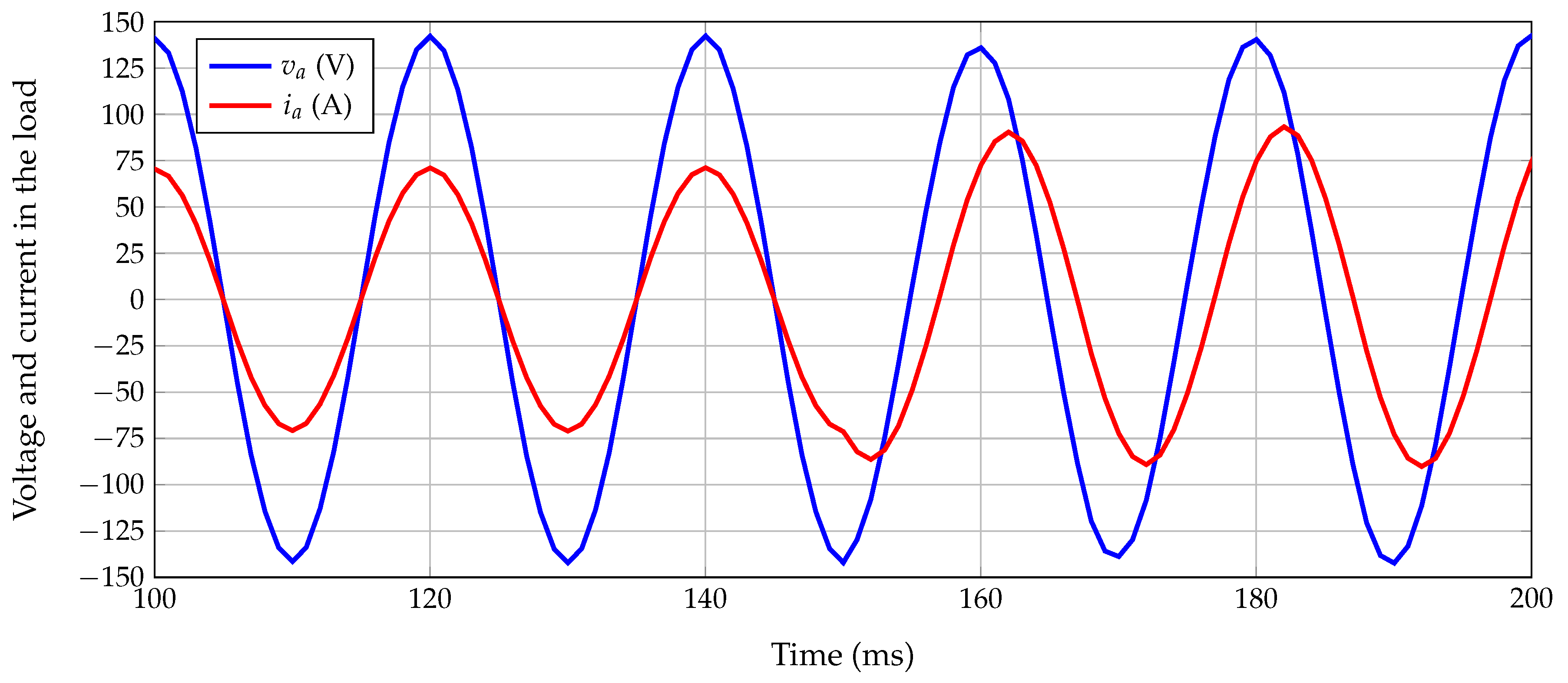
In
Figure 3 the voltage and current profile provided to the
a-phase by the VSC interface to the three-phase load are presented.
Please note that the behavior of the
phase current depicted in
Figure 3 demonstrates that if the voltage profile is supported at the load terminals via passivity-based control as defined in (
11), then, the active and reactive power required by the load is guaranteed. This implies that the power electronic interface presented in
Figure 2 can be used to interface three-phase loads to DC distribution networks with local reactive power support (i.e., unity power factor operation). The main advantage of this interface is that the reactive power is provided locally to the load and no power losses are observed by the DC grid caused by reactive currents, which clearly shows that DC grids are more efficient than AC grids when loads have power factors lower than unity, as it will be presented in section of Results.
5. Test System
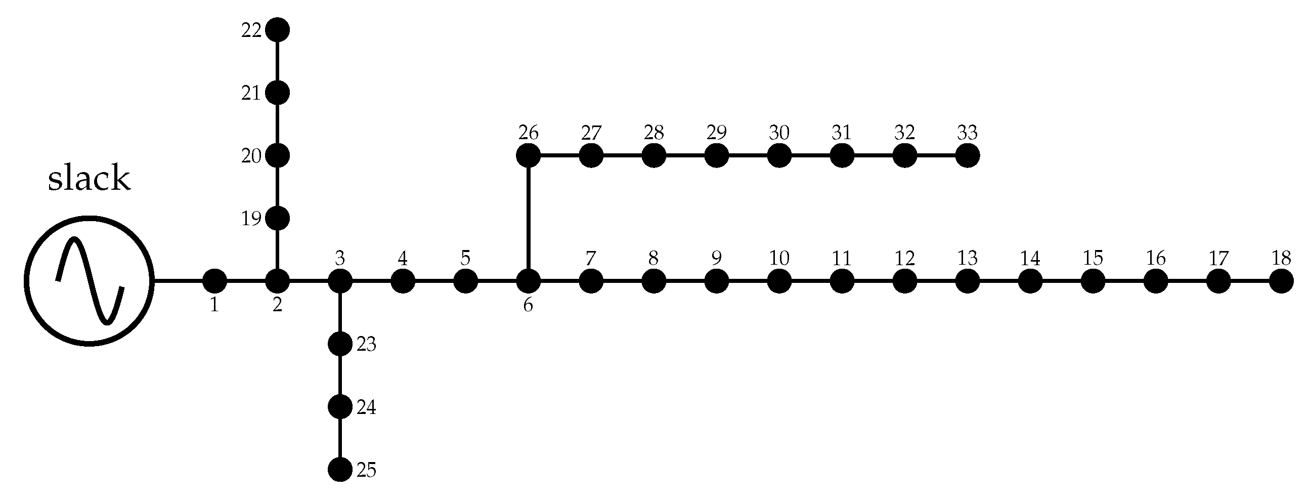
The comparison of the AC and DC technologies for energy distribution in medium-voltage levels is made by using the 33-nodes test feeder reported in [
7]. This test feeder is designed to be operated at 12.66 kV with the connections depicted in
Figure 4. The information regarding branches and loads for this test feeder are reported in
Table 3. Please note that this test feeder corresponds to a three-phase distribution network typically used to study the problem of the optimal location of distributed generators in power distribution networks as reported in [
51].
To evaluate the effect of the renewable generation in the daily operation of this test feeder, we consider four renewable generators previously located in this test system with the information reported in
Table 4.
The connection of the generators for each test system is described as follows: at the node 13 it is connected the photovoltaic generator PV
and the wind turbine WT
with nominal rates of 450 kW and 825 kW, respectively. At the node 25, it is connected a second PV
with a nominal power rate of 1500 kW while at the node 30 it is connected the second wind generator WT
with the nominal capability of 1200 kW. The information regarding battery energy storage systems considered in this test feeder is reported in
Table 5. We assume that the utility has located three batteries, which are distributed as follows: at node 6, a C-type battery is located; at node 14 an A-type battery is used, and at the node 31, a B-type battery is considered.
It is worth mentioning that each one of the renewable source or battery energy storage system corresponds to a DC sub-network interfaced with a power electronic converter that manages the power transferred(absorbed)/to(from) the distribution network regardless whether this is operated under AC or DC paradigm [
3].
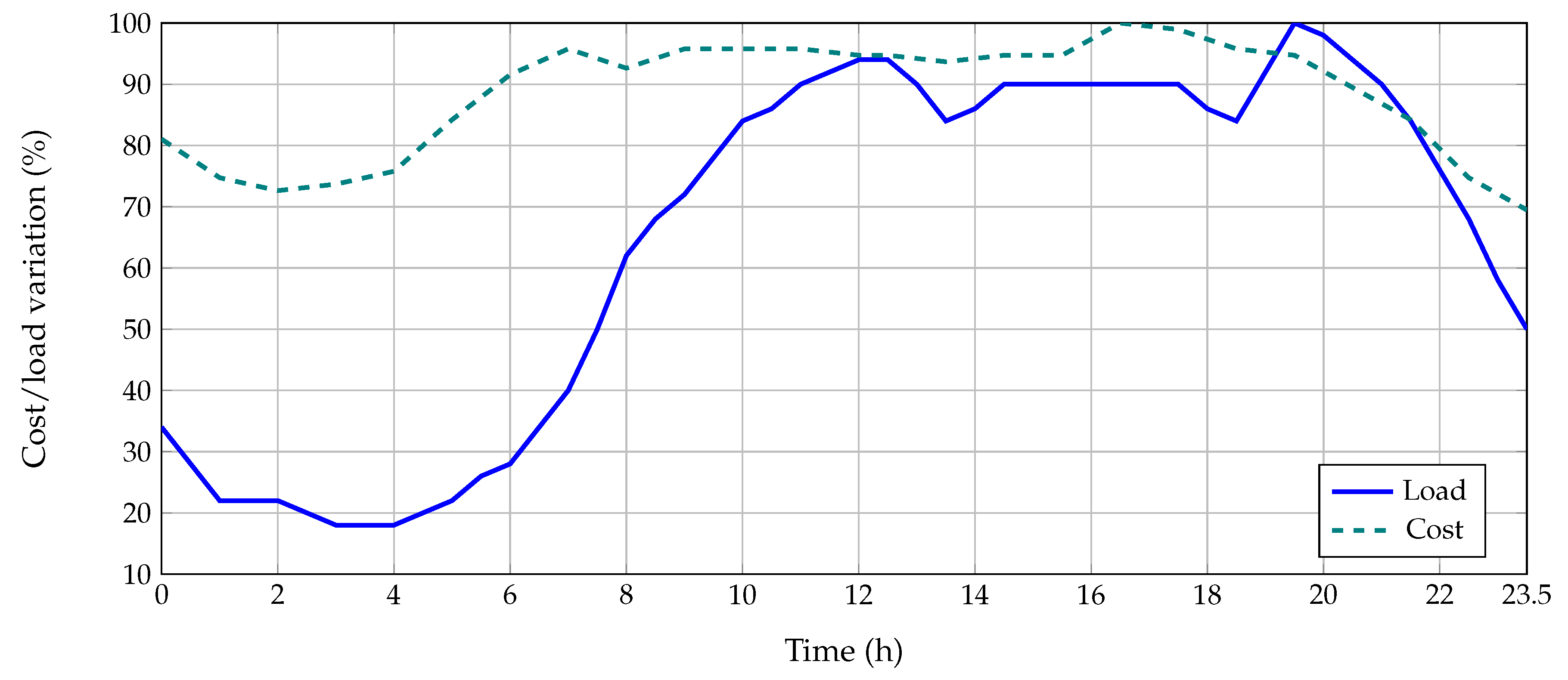
To evaluate the daily variation of the active and reactive power consumption and emulating the hourly price behavior, we consider the load and cost curves reported in
Figure 5. Furthermore, as the peak of the electricity, we assume the information reported by CODENSA utility from Colombia in May 2019, which is COP
$/kWh
.
The numerical information about the demand and cost curves presented in
Figure 5 can be consulted in [
7].
6. Numerical Results and Discussion
In this section, all the numerical results reached by GAMS after implementing the OPF models for AC and DC networks are described. To make a fair comparison between both distribution technologies the following simulation scenarios are proposed:
- ✓
S1: It is considered that the 33-nodes test feeder operates with unity power factor, i.e., all the reactive power consumptions reported in
Table 3 are considered zero in this scenario.
- ✓
S2: The complete information of the 33-nodes test feeder is considered to evaluate the effect of the reactive power demand in the operation of classical AC networks.
It is important to mention that as recommended in [
14] all the batteries start and end the day with
of state-of-charge and during the day (for Ion-Lithium batteries) this variable can be moved from 10% to 90%.
6.1. Operation of the AC Network
In the operation of this grid, we consider three objective functions as follows: Case 1: minimization of the energy losses during the operation horizon, Case 2: the minimization of the energy purchase costs in the conventional generator (node 1) considering the cost curve reported in
Figure 5, and Case 3: the minimization of the total CO
gas emissions in the slack source considering that the 33-nodes test feeder is a rural grid fed by a diesel generator. Here, we consider as reported in [
13] that CO
emission coefficient is 1300 lb/MWh.
Table 6 presents all the numerical results regarding the three objective functions for the S1.
The results in the S1 reported in
Table 6 allows to observe that:
- ✓
The minimization of the energy losses during the day (186.918 kWh/day) implies high costs regarding energy purchase at the slack node (MCOP$9.627). This is a logical result since in this case, the main idea is to define the optimal power injection in renewables (and batteries) and conventional sources to minimize the magnitude of the current flowing through the lines. The energy losses is a function of the square values of the current. Since the objective function is associated with lines the optimization model does not take into account the origin of the energy, which implies that the algorithm chooses whether to purchase energy in the spot market to optimize the objective function regarding energy losses without taking into account its acquisition costs.
- ✓
The second case shows that the minimization of the energy purchase costs in the slack node (MCOP$4.152) is directly related to the minimization of the total gas emissions of CO (13731.976 lb/day) since both are involved with the amount of power injected at this node. Nevertheless, this situation produces the highest energy losses during the operation horizon (449.949 kWh/day). This is explained by the objective function selected since in this case, the goal is to minimize the energy production on the slack node regardless the final magnitude of the current flow through the lines, that accordingly increases the energy losses in the whole system.
- ✓
The third case shows that effectively the energy costs and the amount of CO emissions are correlated objective functions, since minimum values of one of them produces minimum values in the other one with minimal variations; however, this objective function allows reaching a better performance regarding energy losses with 366.155 kWh/day, being an attractive solution since allows to reduce polluting emission gases with low energy purchase costs (MCOP$4.345) and acceptable daily energy losses.
In
Table 7 the numerical results for the S2, i.e., the operation of the 33-nodes test feeder considering active and reactive power consumptions are presented. In general, numerical results presents the same behavior reported in the analysis of the S1. Nevertheless, we can notice that energy losses are drastically affected by the presence of the reactive power consumptions inside of the network. Note that in the first case, energy losses have been incremented at least 5 times in comparison to the unity power factor case. In addition, regarding the minimization of the energy purchase costs in the spot market and the greenhouse gas emissions, the increments are about 1.04 times for both cases, which allows concluding that reactive power practically does not produce effects in those objectives when compared to the operation with unitary power factor.
6.2. Operation of the DC Network
To evaluate the performance of the 33-nodes test feeder, it was considered that the system can be represented by a DC equivalent as defined in the S1. In this sense, the reactive power loads and reactance of this model are removed. The implementation of optimal power flow for this DC medium-voltage distribution network is reported in
Table 8.
From the results reported in
Table 8 we can note that:
- ✓
The behavior of the DC equivalent of the 33-node test feeder (see
Table 8) is identical to the behavior of this system when unity power factor is assigned at all the loads as can be seen in
Table 6. These results imply that when the AC grid is used to support only active power consumption (residential applications), its electrical efficiency is 100% comparable to the emerging DC distribution networks.
- ✓
The only difference between AC and DC distribution considering purely active power consumptions correspond to the need of generating small reactive power quantities in the slack source to support the reactive power losses throughout all the lines. In this context, when the 33-nodes test feeder is operated with unity power factor and considering the minimization of the total energy purchasing costs, the amount of reactive energy generated during the day is about kVAr/day, which needs to be provided by the slack source; while in the DC distribution case this reactive power is inexistent; which can be considered and advantage of the DC technology when compared with the AC counterpart.
6.3. Efficiency Comparison for Different Power Factors
To demonstrate that the DC distribution network is an attractive alternative to provide electrical service to industrial users connected at medium-voltage levels, let us compare the efficiency of this technology with conventional AC grids for different percentages of reactive power consumptions.
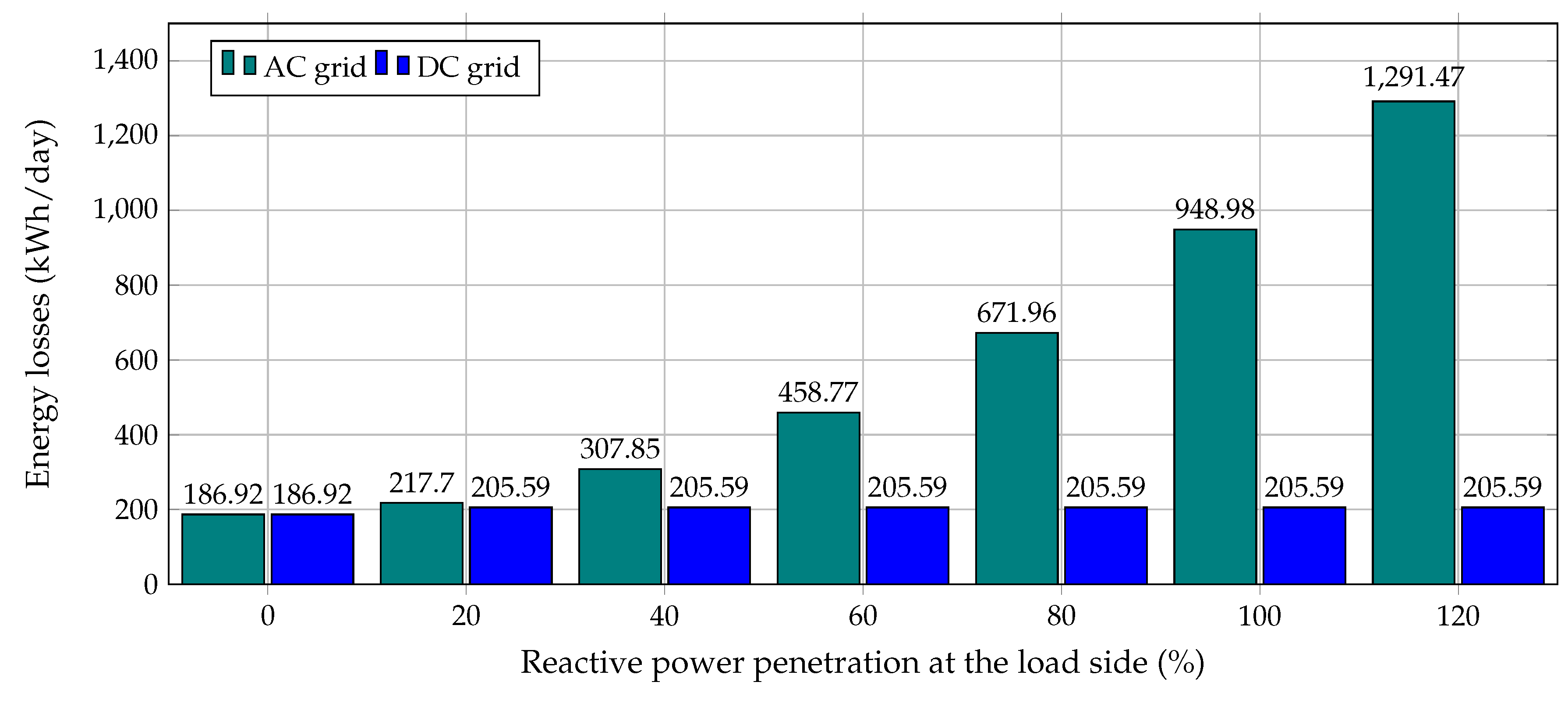
Remark 7. Recall that DC distribution networks are able to provide active and reactive power support to AC loads by using a voltage source converter (VSC) that interfaces the DC grid to the AC load as can be demonstrated in [32], where an isolated (i.e., rural) AC grid receives voltage and power support by interconnecting linear and non-linear loads to DC distribution grids via a VSC. In
Figure 6 it is presented the amount of energy losses (objective function minimize) in the AC grid when the reactive power load changes from 0 to 120% of the peak value reported in
Table 3; in addition, the total energy losses are also presented in the DC equivalent network, assuming that the energy losses at all the VSCs are about 10% of the total energy losses of the network. Please note that in the case of the DC grid the reactive power is provided directly at the load side, which implies that this power is provided by the power electronic interface as explained in
Section 4. For this reason, the active power losses for DC grids remains constant for different percentage of reactive power demands at the load side, since no currents are associated with this power flow in DC distribution lines.
The information regarding daily energy losses in the AC and DC equivalent networks make evident that the efficiency of the AC grid is deteriorated rapidly as a function of the amount of reactive power consumption at all the loads due to the exponential increment of the total energy losses. Nevertheless, in the case of the DC network the efficiency is always constant regardless the reactive power consumption. This is explained by the fact that the VSCs that interface the AC loads are able to locally generate reactive power, which implies that the DC distribution makes the node can sense their effects in its lines. Please note that when the loads in the 33-nodes test feeders are 100% reactive power consumption, the AC grid has kWh/day of energy losses, while in the case of the DC equivalent these losses are about kWh/day. These results imply that the AC grid has at least 4.6 times more energy losses than the DC equivalent, which confirms that the DC technology is a promissory alternative to provide the electricity service at medium- and low-voltage distribution levels with higher efficiency levels regarding energy losses, compared at the distribution stage, i.e., involving energy losses in conductors used in the electricity distribution. It is important to mention that this high relation (i.e., 4.6 times for the 33-nodes test feeder) is largely influenced by the relation between active and reactive power demand in the distribution network under study. This implies that this data can be considered to be an indicator, but more studies regarding energy efficiency at all the electronic interfaces (renewable generators, energy storage devices and controllable loads) are needed to determine the overall energy efficiency at distribution levels.
6.4. Effect of Renewable Energy Variations in the Economic Dispatch
In this subsection it is explored the possible operation scenario where renewable energy has important variations regarding weather conditions such as cloudy and rainy days, including very low-speed winds. In this case, we consider as objective function the total energy losses minimization during daily operation, i.e., the Case 1. To consider all the possible operation scenarios in a real network, we consider that the amount of renewable energy varies from 0% to 100% in steps of 20%. In addition, we consider that all the loads in the 33-nodes test feeder operate under normal conditions, i.e., 100% of active and reactive power consumption.
Table 9 presents the behavior of the AC and DC distribution networks when there are higher variations in renewable energy production.
From results reported in
Table 9 we can observe that: (i) the difference regarding daily energy losses between AC and DC grids remains practically constant with an average value of
kWh/day. This implies that at all the possible renewable energy penetration scenarios the DC grid has better behavior in terms of grid energy losses, which can be explained by the possibility to provide local reactive power with the VSC interface. This latter is not the case of the AC grid where the reactive energy flows from the substation to the loads; (ii) the division between the DC and AC energy losses presented in the last column of
Table 9 shows that the efficiency of the DC grid in comparison to the AC case increases as a function of the renewable energy penetration in the grid; this behavior is mainly associated with the important reductions in the power flow through the lines caused by local injections of active power by renewable sources; and (iii) the total energy reduction in the AC grid when renewable energy penetration passes from 0 % to 100% is about
, while in the case of the DC network this reduction is about
, which entails that the same level of renewable energy penetration provides more positive impacts in a distribution network designed under the DC paradigm in contrast with the conventional AC grids.
7. Conclusions and Future Works
A comparative study regarding energy efficiency in AC and DC electrical networks for power distribution from the point of view of optimal power flow analysis was presented in this paper. This study allowed to confirm that AC and DC technologies have identical performances in residential applications, i.e., unity power factor, since the amount of energy losses, greenhouse gas emissions of CO or energy purchase costs are practically the same for both technologies. Nevertheless, in the case of high penetration of reactive power consumptions in AC networks (mainly in industrial applications), it was demonstrated that the performance of the AC grid is rapidly deteriorated compared with the DC equivalent, due to the need to transport this reactive power from the substation towards the loads. This increases the magnitude of the current through the lines, being translated into higher energy losses during the operation horizon. This situation does not happen in the case of the DC grids where reactive power is directly provided by the VSCs that interfaces all the AC loads, which implies that the efficiency of the DC distribution system remains constant regardless the reactive power requirements of the load.
To solve the optimal power flow models regarding the daily operation of AC and DC grids, we have introduced the GAMS software to efficiently solves both models with low computation effort, i.e., processing times about 5 s in all the simulation cases and scenarios. This low-computational time is important since multiple simulation cases can be analyzed before taking the final decision in regards with the day-ahead economic dispatch environment, which makes the GAMS software an attractive alternative for tertiary control in distribution networks. In addition, the GAMS package is a proper tool to solve complex optimization problems by focusing the attention on correctly developing the optimization models rather than the solution technique. This represents an ideal framework to easily introduce engineers and researchers in mathematical optimization; for this reason, this paper has been addressed in a tutorial form.
As future work it will be possible to analyze the following problems: (i) propose convex reformulations for optimal power flow analyses in AC and DC networks that will ensure reaching the global optimum of the problem under well-defined operative conditions, which are very attractive for real economic dispatch applications, (ii) make a comparative study between AC and DC grids considering transient operation scenarios such as suddenly load disconnections or short-circuit cases, which can be used in protective devices coordination studies for these grids, and extend the economic dispatch optimization model to three-phase distribution networks and bipolar DC configurations operated under unbalanced loads scenarios to analyze their efficiency in terms of power losses and voltage profiles.


