Abstract
Adversarial examples are theorized to exist for every type of neural network application. Adversarial examples have been proven to exist in neural networks for visual-spectrum applications and that they are highly transferable between such neural network applications. In this paper, we study the existence of adversarial examples for Infrared neural networks that are applicable to military and surveillance applications. This paper specifically studies the effectiveness of adversarial attacks against neural networks trained on simulated Infrared imagery and the effectiveness of adversarial training. Our research demonstrates the effectiveness of adversarial attacks on neural networks trained on Infrared imagery, something that hasn’t been shown in prior works. Our research shows that an increase in accuracy was shown in both adversarial and unperturbed Infrared images after adversarial training. Adversarial training optimized for the norm leads to an increase in performance against both adversarial and non-adversarial targets.
1. Introduction
Surveillance is a common application of Infrared cameras and the detection/recognition tasks in the electromagnetic band are common in military and surveillance applications. Low-wave Infrared (LWIR) and Mid-wave Infrared (MWIR) are used in military applications such as Night Vision, missile targeting, and computer vision applications including tracking. Real-time operations such as tracking work through running an object recognition algorithm on frames of a video. This is resource-intensive, there are multiple applications that are not running live but instead on a few seconds of delay because of intensive CPU/GPU memory usage. Computer vision algorithms rely on numerous attributes of an image that a human processing the image may take for granted. Images in Infrared and the Visual spectrum differ in many of these attributes. Information that is shown in the Visual such as reflectively, luminescence, color, and texture, is lost either partially or entirely when looking at the same object in the Infrared spectrum. This is the motivation of this paper showing that exploiting the gradients of an image can be an effective attack against computer vision models for surveillance trained on Infrared imagery and that the same defenses being deployed for models trained for the visual spectrum can be deployed models trained for the Infrared spectrum.
Adversarial training is a simple training method to diminish the success of adversarial attacks. This technique augments training data with adversarial examples created from the model. The ensemble adversarial training method used by Tramer et al. in 2018 was used to diminish the success of transferred adversarial examples [1]. This technique augments training data with adversarial examples created from other models and or adversarial examples created to attack this specific network, to harden algorithms against transferred adversarial examples. Adversarial training is optimized against one of the three image attack distances, , , . For this investigation, we explore adversarial training optimized for the distance.
This paper studies the existence of adversarial examples for Infrared neural networks that are applicable to military and surveillance applications which are based on Infrared images and use neural networks for detecting anomalies. Our study shows that adversarial training alleviates the problem and creates robustness in models against similar adversarial examples. Adversarial training optimized for the norm leads to an increase in performance against both adversarial and non-adversarial targets.
Our investigation is novel because of its finding in regard to neural networks trained on Infrared imagery. Prior to our work, no published research has shown the effectiveness of adversarial attacks on neural networks trained on 1 channel unique imagery. Our work also shows the effectiveness of adversarial training for neural networks retrained and trained from scratch on Infrared imagery which addresses vulnerabilities in neural networks in current use for military applications. Standard RGB images are composed of three channels of pixel information. Each of these channels correspondingly represents red, green, and blue, respectively. The overlapping of the channels imitates visual light. Infrared images in low wave and mid-wave are longer in wavelength and are one-channel images.
As discussed in Section 2, while there has been research into both adversarial examples transferability, adversarial examples using the fast gradient sign method, and also Infrared models viability and performance, no research has been done to establish that adversarial attacks work for Infrared models and also that robustness of Infrared models can be improved using adversarial training. This work aims at proving both the viability of adversarial attacks on Infrared models and also the value of adversarial training on Infrared models.
2. Related Work
Research in [2] has introduced the idea of adversarial examples and named them perturbations, as well as the idea of tranferability. Authors have concluded that neural networks that learn through back-propagation share non-intuitive characteristics and blind spots. Consequently, the same adversarial example can be very effective on multiple models trained on different sets of data. This work was done using the MNIST Digit dataset with different subsets of 30,000 training images [3]. Adversarial examples for one neural network are still statistically hard for another neural network trained on a different subset of data or with different hyperparameters.
An ensemble method of adversarial training that augments training data with adversarial examples transferred from other models has been introduced in [1]. Similarly, the work in [4] has extended the application of adversarial examples to edge detection and boundary detection for images [4]. The research work in [5] has explained the underlying reasons behind the high transferability we see from model to model in regard to adversarial examples [5].
Zhao et al. in their research tested transferability to other black box models such as Faster RCNN, YOLO v3, SSD RCNN, and Mask RCNN [1,6,7]. These nested adversarial examples used image transformation techniques to simulate varying factors, and their introduction of batch-variation momentum training increased the transferability of their adversarial examples [6]. The work in [8] has studied why obfuscating the gradients of an image does not stop attackers from successfully attacking a model. The research work in [9] introduced methods to interpret adversarial training such as Total Variation regularization and Lipschitz regularization. The work in [10] has introduced several attacks that perform better than Fast Gradient Sign method (FGSM) according to the , , metrics.
3. Proposed Approach
Our approach to understanding the effectiveness of adversarial training for Infrared images was tri-fold. In order to ensure that our model complexity didn’t cause the change in accuracy after adversarial training two separate neural architectures, one a simple 8-layered neural network that would be trained from the ground up with empty weights. The other network would be pretrained on a benchmarked ResNet50 algorithm to ensure that a comparison could be made with benchmarked RGB datasets, and that a complex model or deep neural network would be shown to have similar results. Our second experimental axis was using both RGB and Infrared data to train separate models. Each architecture was used to train two separate models one trained using RGB data and the other Infrared data. The RGB ResNet50 model being the only model that didn’t need to be trained before testing effectiveness on unperturbed test images. The dataset used was the CIFAR-10 dataset a dataset comprised of 10 separate classes of images with 6000 per class. A grayscale and contrast intensity along with Gaussian filtering, and lastly a concatenation into one channel was done to create simulated Infrared version of the CIFAR-10 dataset. An upsampled example of this is shown in Figure 1. Both architectures were then tested on imagery from the test sets, benchmarked, then tested on adversarial images created using the PGD attack and benchmarked again. The models were then retrained using Adversarial training, and benchmarked once again on unperturbed and perturbed imagery. Both models were then tested on perturbed and non perturbed Infrared images from the VAIS dataset which contains images of ships in Infrared [11]. An example of an image from the VAIS dataset is shown in Figure 2.
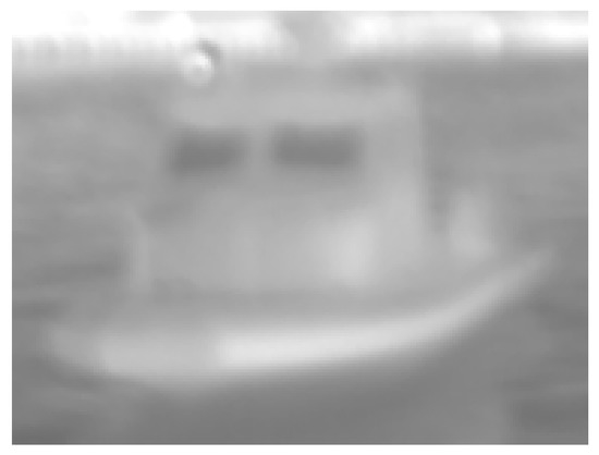
Figure 1.
CIFAR-10 simulated LWIR ship
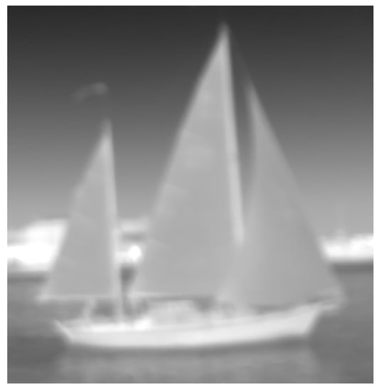
Figure 2.
VAIS LWIR ship.
4. Brief Overview of Neural Network
Neural networks are modeled to behave similarly to human or intelligent animal brains. Models are able to learn tasks without being hard-coded and generally improve performance the longer they ‘train’. A neural network is a layered network of neurons that are connected, and each of them weighted. Hyperparameters that are defined before the network starts to train can have an effect on the performance of the network. Weights are updated in the network through backpropagation. The output of the network is some statistical distribution of classes, although this can be expressed in multiple ways. Deep neural networks (DNN) are characterized as having many layers of neurons and must use propagation to update weights of the network due to their size; all state-of-the-art DNN’s use backpropogation [7,12,13].
4.1. System Flow Model
A typical system model is shown in Figure 3, where data and some perturbation are input into the learning/predicting model that gives the (mis-)classification.
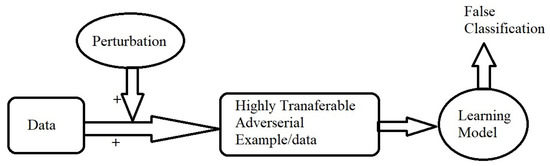
Figure 3.
System/flow model.
For some target model and inputs, the adversary’s goal is to find an adversarial example such that and x are “close”, yet the model misclassifies . Given some budget , output examples where .This is exemplified in both the targeted and non targeted equations in Section 4.1.4 and Section 4.1.5.
The L-norms are calculated as below [10].
- metric The distance metric measures the number of coordinates in an image and its adversarial perturbed counterpart that is not equal:
- metric: The distance metric measures the Euclidean distance between an image and its adversarial perturbed counterpart:
- metric The measures the maximum change between any of the pixels between an image and its adversarial perturbed counterpart:
4.1.1. White Box Scenarios
A white box attack is defined as an attack in which an attacker has complete access to the model being attacked [14]. The FGSM is a proven, but, most importantly, fast attack for this scenario. This optimizes for the metric. The attacker can use the gradients to surf towards an optimal perturbation for this model. Since the attacker has access to the loss landscape, they can use this information to attack the input gradients and maximize loss on the adversarial example with the original class and minimize loss with the intended target class if the attack is targeted [5,8,14]:
4.1.2. Black Box Scenarios
A black box attack is defined as an attack in which the attacker does not have access to the model itself but only endpoints such as an API that accepts inputs and returns: outputs to the model. The attacker may not have access to a probabilistic output from the model either. The model may output the highest likelihood class only; in this case, the attacker doesn’t get feedback. Momentum training can be used in cases where the model gives a probabilistic output.
In situations where the attacker is deprived of multi-class output or gradient masking is being used, the attacker can use an adversarial example created to work on a simpler model trained by the attacker themselves that aligns with the target model. Zhao et al. in their research tested transferability to other black box models such as Faster RCNN, YOLO v3, SSD RCNN, and Mask RCNN [1,9,15]. These nested adversarial examples used image transformation techniques to simulate varying factors, and their introduction of batch-variation momentum training increased the transferability of their adversarial examples [6].
4.1.3. Targeted vs. Non-Targeted Examples
An adversarial example is simply an input that forces a misclassification. The attacker reaches its goal by merely forcing the source input to misclassify [1,14,16]. This can be achieved through the attacker, abusing the input gradients.
Adversarial inputs can be invisible to the human eye but are visible to the neural networks or computers, which use pixel value and gradients between pixels to perform recognition tasks. Changing the value of one pixel in an image may result in a higher probability of another class prediction. In this way, attackers can use gradients to attack the network. The same techniques that work to attack neural networks that use RGB data can be used to attack neural networks that use Infrared data. The Infrared image can be interpreted as a one channel image containing pixels with values between black and white, with white meaning high radiation and black, meaning no radiation.
Adversarial attacks work regardless of the data set that the model is trained to recognize. Object recognition models are not prophetic oracles that have infinite knowledge on a particular subject but instead should be thought of as machines meticulously trained on recognizing features of a particular set of classes. Each class can be thought of as a combination of weighted scores of particular features within the feature space. Slight deviations of scored features on inputs can lead to a different output mapping. Attackers attack the gradients of a network in order to gain their desired misclassification.
4.1.4. Non-Targeted
- –
- x: Input image
- –
- : Adversarial Image
- –
- J: Loss Function
- –
- : Model Output for x
- –
- : Tuneable parameter
An example in which an adversarial image meets the requirements of misclassifying the source image, but in any vector. Any class ỹ is a optimal for the attacker. The adversarial image being represented by . The attacker does not care what the output class is as long as it is different then the original class. The attacker maximizes the loss of the true label to gain any label other than it.
4.1.5. Targeted
- –
- x: Input image
- –
- : Adversarial Image
- –
- J: Loss Function
- –
- : Targeted output
- –
- : Any class that isn’t targeted
- –
- : Tunable parameter
A targeted example is one in which a specific class is targeted as output [1,14,17]. In the targeted scenario, the attacker chooses a target class, and maximizes the loss of the true label while minimizing the loss of the target label. This can be achieved by maximizing the loss of all classes not equal to the target label while minimizing loss of the target label.
4.2. Attacks on Images
Ian Goodfellow first introduced the FGSM attack in 2015 [14]. The FGSM attack uses the optimized gradients of a model to determine a direction towards a maximum. In an enclosed system where the input in is an image and the output is the probability of this image belonging to each of five classes. Using this information as feedback, an attacker is able to exploit the gradients of the Neural network to travel in the direction of their desired classification [14]. An example of MNIST is shown in Figure 4.
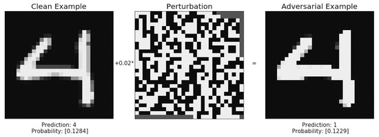
Figure 4.
An MNIST (Modified National Institute of Standards and Technology) example.
An example of adversarial attack and Gradient masking is shown in Figure 4.
Gradient Masking was proposed as a method that could make it difficult for an attacker to implement the optimized gradients attack. Any small perturbation is treated as the same example; this does not provide useful gradients for the attacker to derive a direction to update pixels [18]. The attacker can still discover these directions by other means, such as using adversarial examples that affect a smooth model. This defense, which was shown to be ineffective by Nicolas Papernot in 2016 [18], fails to improve the robustness of the model itself.
4.3. Transferability
The term transferability in terms of adversarial examples means the ability for valid adversarial examples created from one model to work on other models. A common approach of creating a network is to use transfer learning to reduce the costs of data collection, shorten the often lengthy training process, and also to have a starting point that is bench-marked [10]. Data is precious in machine learning; it is expensive in terms of resources to collect and label; therefore, it is common for different algorithms to be trained on variations of the same data. The rise of transfer learning, which speeds up the process of training a network and lessens the amount of computation needed to get a highly efficient neural network, leaves many neural networks with similar complexities [5,19].
The size of input gradients, the variance between the surrogate and target models, and also the variance of the loss landscape were found to be critical factors in the success of transfer attacks [5]. Numerous open-source algorithms have been tested with adversarial examples. Faster-RCNN has been cracked using ShapeShifter digital perturbations again created with a gradient optimization [14]. These attacks were transferable to Inception V2, ResNet v2, and SSD-MobileNet v2 models. Further research is yet to be done on universal transferability, as shown in Figure 5 (e.g., [20]).
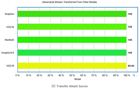
Figure 5.
Transferability of adversarial attacks in machine learning from other models.
4.3.1. Possible Defenses
Potential defenses of adversarial attacks include adversarial training—in which adversarial examples are included in the training of the algorithm. Although this is still vulnerable to adaptive attack, this may be solved by using a GAN or similar continuous training approach to incorporate more and more examples into the network [15]. Obfuscation of gradients in a model’s output, by only showing top-1 class, can slow down an attacker, but doesn’t dissuade a savvy attacker and is therefore not recommended as a defense from adversarial attacks [8].
It is assumed that the attacker has knowledge of what classes the network is trained on or at least general knowledge about the data that the classifier was trained on, and also access to the trained algorithm itself for performing the attack. For the attack performed in this research experiment, access to the training data, in this case, images, is vital in order to exploit gradient changes in the images. However, an attacker only needs to know of the classes that the model is trained on and can then grab any image of said target class to create an adversarial image by cross-referencing the new image with the output of the model fed said image as an input.
4.3.2. Description of the Solution
While FGSM makes the assumption that linear approximations for x can be used to make an approximation of a region that is fast, the flaw with approach is that neural networks aren’t linear in even small regions [21]. The PGD or Projected Gradient Descent instead maximizes the loss function rather then performing gradient steps [21]. The intuition being that adding perturbed images to the training dataset that the model is trained on adds robustness to the model. The robustness of the model after training depends on the strength of the adversarial examples used in training [10,14,22]. The defense optimizes the total amount pixels that were changed in the image.
The PGD attack is implemented for each image with a label pair in the batch. For each clean image in that minibatch, an adversarial image is created and added to the minibatch. After the creation of the adversarial data set, the model is retrained and the loss of the model is improved on using backpropagation [10,21,22]. The Adversarial training algorithm used is shown Algorithm 1. This is expanding the range of pixel values that the model is accepting as the label. The model is thus hardened against attacks against the norm.
| Algorithm 1: Adversarial Training with PGD attack |
|
- –
- x: Input image
- –
- : Adversarial Image
- –
- J: Loss Function
- –
- : True Label
- –
- : Any class that isn’t targeted
- –
- : Tunable parameter
4.3.3. Comparison to Other Related Works
The results of this simulated Infrared dataset were compared to the CIFAR-10 dataset and also the MNIST dataset. The MNIST dataset is comprised of the 10 Arabic digits drawn from a multitude of angles. The CIFAR-100 dataset is composed of 100 classes of everyday objects, animals, and vehicles. As a proxy for an Infrared dataset, this work augmented the CIFAR-10 dataset, which is a subset of the CIFAR-100 dataset and a grayscale of all of the images. Results of the adversarial training have been shown to vary in experiments of Madry [10] and also Shafahi [22]. Researchers in the past have benchmarked the ResNet22 architecture at 200 epochs for the CIFAR-10 dataset at a 92.16% accuracy [23]. Using this benchmark, our research shows the accuracy of an adversarial attack against this model using the PGD attack. The ResNet22 architecture was then trained for the simulated Infrared CIFAR-10 dataset. Our models have also been tested against Infrared images of Ships from the VAIS dataset. This dataset contains hundreds of images of ships from differing distances, and angles taken in LWIR [11].
5. Performance Evaluation: Results and Discussion
To be able to compare the results of adversarial training ofsimulated Infrared images, a control CNN was also run using the CIFAR-10 dataset without grayscale augmentation. Adjusting Infrared images via prepossessing is a common practice, due to the low pixel values and small gradients between pixels, contrast adjustment and histogram, and the highlights bring out information in the images that would be hidden without adjustment.
The simulated Infrared CNN shown in Figure 6 before adversarial training was 49% accurate on the test set and 11% accurate when testing against adversarial images. After adversarial training, the IR CNN improved by 13% to 60% accurate on the test set while being 46% accurate when testing on adversarial images, a full 35% increase in accuracy against adversarial images. The control CNN shown in Figure 7 achieved 55% test accuracy and 10% accuracy against adversarial images before adversarial training. After adversarial training, the control achieved 75% test accuracy and 50% accuracy against adversarial images.
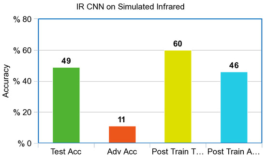
Figure 6.
Accuracy with a simulated Infrared Model for CNN.
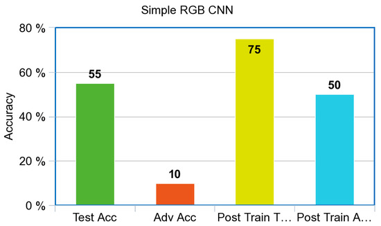
Figure 7.
Accuracy with an RGB Model for CNN.
The Infrared CNN shown in Figure 6, and the RGB CNN shown in Figure 7, performed poorly against adversarial examples created via the PGD attack prior to adversarial training. Both models improved dramatically from adversarial training, a 35% increase for the simulated Infrared model with a final adversarial test accuracy of 46%; the control model increased from 10% accuracy to 50% accuracy against adversarial images. Surprisingly, both models also increased overall accuracy against the test set after adversarial training. The Infrared CNN model trained on simulated images also showed an increase in performance on our Infrared dataset of ships from VAIS, an increase of 11% on unperturbed images, and an increase of 40% on Adversarial images, as referenced in Figure 8.
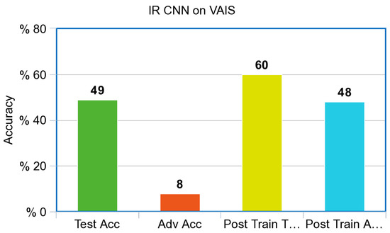
Figure 8.
CNN Infrared Model accuracy on the VAIS Infrared dataset.
Additionally adding more epochs to the training can cause over-fitting of the model, an inflection point where performance degrades.
The simulated Infrared ResNet model shown in Figure 9 was pretrained on the CIFAR-10 dataset and then retrained on the simulated Infrared CIFAR-10 dataset. Two hundred epochs were used as a hyperparameter for models based on ResNet architecture. This allowed a fair comparison to the published benchmarked ResNet model trained on the CIFAR-10 dataset. The model achieved a 75.82% test accuracy after initial training. Adversarial examples were correctly labeled with a 12.19% accuracy before adversarial training. After adversarial training, the model was able score a test accuracy of 83.13% training on the non-adversarial test set, and 69.13% accuracy on the adversarial test set.
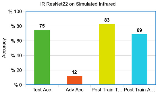
Figure 9.
Accuracy with an Infrared model for ResNet.
The pre-trained ResNet model is shown in Figure 10. On the RGB test set, the benchmark level of accuracy in literature was 92%. As expected, the model accuracy drastically decreased when adversarial images were introduced. ResNet accuracy for the adversarial examples produced by the PGD attack was 14.6%. After adversarial training, the test accuracy of the ResNet model increased roughly 2% for a total accuracy of 94.56% and an adversarial accuracy of 85.7%.
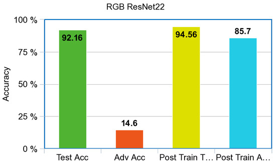
Figure 10.
Accuracy for the RGB Model for ResNet.
Both the simulated Infrared and the RGB ResNet models showed improvement after adversarial training. This result is in accordance with the smaller simple CNN’s that were trained from scratch. One major difference that can be noted between both model architectures is the number of layers and the initial test accuracy. The RGB CNN performed quite poorly on a dataset that has been benchmarked by sophisticated DNN’s such as the ResNet at extremely high accuracy. Even small performance gains for a DNN such as ResNet are valuable. If one can afford to do the computation, it is worth doing.
Both the simulated Infrared and RGB ResNet models also showed drastic improvement on the adversarial test set after adversarial training. This shows that they are in accordance once again with the results from the simple CNN that were created for the experiment. The Infrared ResNet model trained on simulated images also showed an increase in performance on our Infrared dataset of ships from VAIS, an increase of 6% on unperturbed images, and an increase of 58% on Adversarial images, as referenced in Figure 11.
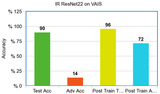
Figure 11.
ResNet Infrared Model accuracy on the VAIS Infrared dataset.
The difference in computation time necessary for the two model architectures to be trained was drastic. This is mostly due to the size of both networks and also the number of epochs used by both models. A simple CNN was run for 20 epochs while the ResNet model was trained for 200 epochs as dictated by its paper. The Resnet archictecture performed better with increased epochs, while the simple CNN architecture overfit after 20 epochs. All other hyperparameters for the experiments were kept the same with respect to each model architecture. The results also show that, while in the RGB spectrum ResNet outperformed the CNN, in the IR part of the spectrum, there was a large difference in performance after adversarial training. The difference in performance is exemplified in Figure 6, and the IR ResNet model shown in Figure 9 is within 11% points.
6. Conclusions and Future Work
This research tested the validity of adversarial examples in neural networks trained on Infrared images. Adversarial training resulted in a significant increase in performance in terms of accuracy against adversarial test sets and unperturbed test sets. Adversarial training resulted in an 11% increase in accuracy for the Infrared CNN tested on unperturbed images and a 35% increase in accuracy on adversarial test images. We observed that the adversarial training for the RGB CNN led to a 20% increase in accuracy against unperturbed images and a 40% increase in accuracy against adversarial images. As for the ResNet model trained for the experiment, adversarial training led to a 2% increase on the unperturbed images and a 70% increase in accuracy against adversarial test images. The ResNet model showed similar results to the simple CNN that was trained in accordance with the IR model. While starting off at a higher initial accuracy of 75%, a near 10% increase was achieved after adversarial training on unperturbed images. On adversarial images, the ResNet model showed a 12% accuracy on the adversarial test set while a 69% accuracy on the adversarial test set after adversarial training. Our models trained on simulated Infrared imagery also generalized well on Infrared images from the VAIS dataset. Models adversarially trained also showed improved performance on actual LWIR images.
As stated in the objectives, this experiment shows the drop-off in performance on neural networks trained on RGB data and simulated Infrared data. For both simple and complex models trained on simulated Infrared data, a substantive increase in accuracy was achieved. The simulated Infrared CNN model achieved a final accuracy of 60%. The same CNN architecture trained on RGB data achieved a final accuracy of 75%. Furthermore, the experiment results showed a drop in performance on neural networks trained on RGB data and simulated Infrared data. For both simple and complex models trained on simulated Infrared data, a substantive increase in accuracy was achieved. The simulated Infrared CNN model achieved a final accuracy of 60%. The same CNN architecture trained on RGB data achieved a final accuracy of 75%.
The adversarial images created with the PGD attack worked just as theorized in the case of both the RGB and FGSM models. Adversarial training optimized for the metric proved to increase accuracy in both unperturbed and perturbed images; this study proves that adversarial training increases model robustness for both deep and simple model architectures for simulated Infrared and RGB data.
Author Contributions
Data curation, D.E.; Formal analysis, D.E. and D.B.R.; Funding acquisition, D.B.R.; Investigation, D.B.R.; Methodology, D.E.; Supervision, D.B.R. All authors have read and agreed to the published version of the manuscript.
Funding
This work is partly supported by the U.S. Air Force Research Lab (AFRL), the U.S. NSF under grants CNS 1650831 and HRD 1828811, and by the U.S. Department of Homeland Security under grant DHS 2017-ST-062-000003.
Acknowledgments
This work is partly supported by the U.S. Air Force Research Lab (AFRL), the U.S. NSF under grants CNS 1650831 and HRD 1828811, and by the U.S. Department of Homeland Security under grant DHS 2017-ST-062-000003. However, any opinions, findings, and conclusions or recommendations expressed in this document are those of the authors and should not be interpreted as necessarily representing the official policies, either expressed or implied, of the funding agencies.
Conflicts of Interest
The authors declare no conflicts of interest.
References
- Tramer, F.; Kurakin, A.; Papernot, N.; Goodfellow, I.; Boneh, D.; McDaniel, P. Ensemble Adversarial Training: Attacks In addition, Defenses. arXiv 2018, arXiv:1705.07204. [Google Scholar]
- Szegedy, C.; Zaremba, W.; Sutskever, I.; Bruna, J.; Erhan, D.; Goodfellow, I.; Fergus, R. Intriguing properties of neural networks. arXiv 2013, arXiv:1312.6199. [Google Scholar]
- LeCun, Y. The MNIST Database of Handwritten Digits. 1998. Available online: http://yann.lecun.com/exdb/mnist/ (accessed on 4 December 2019).
- Cosgrove, C.; Yuille, A.L. Adversarial Examples for Edge Detection: They Exist, and They Transfer. arXiv 2019, arXiv:1906.00335. [Google Scholar]
- Demontis, A.; Melis, M.; Pintor, M.; Jagielski, M.; Biggio, B.; Oprea, A.; Nita-Rotaru, C.; Roli, F. Why Do Adversarial Attacks. In 28th USENIX Security Symposium (USENIX Security 19); USENIX Association: Santa Clara, CA, USA, 2019; pp. 321–338. [Google Scholar]
- Zhao, Y.; Zhu, H.; Liang, R.; Shen, Q.; Zhang, S.; Chen, K. Seeing isn’t Believing: Practical Adversarial Attack Against Object Detectors. arXiv 2019, arXiv:1812.10217. [Google Scholar]
- LeCun, Y.; Bengio, Y. Convolutional networks for images, speech, and time series. Handb. Brain Theory Neural Netw. 1995, 3361, 1995. [Google Scholar]
- Athalye, A.; Carlini, N.; Wagner, D. Obfuscated gradients give a false sense of security: Circumventing defenses to adversarial examples. arXiv 2018, arXiv:1802.00420. [Google Scholar]
- Carlini, N.; Wagner, D. Towards evaluating the robustness of neural networks. In Proceedings of the IEEE Symposium on Security and Privacy, San Jose, CA, USA, 22–26 May 2017. [Google Scholar]
- Madry, A.; Makelov, A.; Schmidt, L.; Tsipras, D.; Vladu, A. Towards deep learning models resistant to adversarial attacks. arXiv 2017, arXiv:1704.08847. [Google Scholar]
- Zhang, M.M.; Choi, J.; Daniilidis, K.; Wolf, M.T.; Kanan, C. VAIS: A dataset for recognizing maritime imagery in the visible and infrared spectrums. In Proceedings of the 2015 IEEE Conference on Computer Vision and Pattern Recognition Workshops (CVPRW), Boston, MA, USA, 7–12 June 2015; pp. 10–16. [Google Scholar]
- Domhan, T.; Springenberg, J.T.; Hutter, F. Speeding up automatic hyperparameter optimization of deep neural networks by extrapolation of learning curves. In Proceedings of the Twenty-Fourth International Joint Conference on Artificial Intelligence, Buenos Aires, Argentina, 25–31 July 2015. [Google Scholar]
- Hecht-Nielsen, R. Theory of the backpropagation neural network. In Neural Networks for Perception; Elsevier: Amsterdam, The Netherlands, 1992; pp. 65–93. [Google Scholar]
- Goodfellow, I.J.; Shlens, J.; Szegedy, C. Explaining In addition, Harnessing Adversarial Examples. arXiv 2015, arXiv:1412.6572. [Google Scholar]
- Qin, Y.; Carlini, N.; Goodfellow, I.; Raffel, G.C.C. Imperceptible, Robust, and Targeted Adversarial Examples for Automatic Speech Recognition. arXiv 2019, arXiv:1801.01944v2. [Google Scholar]
- Goodfellow, I.; Pouget-Abadie, J.; Mirza, M.; Xu, B.; Warde-Farley, D.; Ozair, S.; Courville, A.; Bengio, Y. Generative adversarial nets. arXiv 2014, arXiv:1406.2661v1401. [Google Scholar]
- Baluja, S.; Fischer, I. Adversarial transformation networks: Learning to generate adver-sarial examples. arXiv 2017, arXiv:1703.09387. [Google Scholar]
- Papernot, N.; McDaniel, P.; Goodfellow, I.; Jha, S.; Celik, Z.B.; Swami, A. Practical Black-Box Attacks against Machine Learning. arXiv 2016, arXiv:1602.02697. [Google Scholar]
- Petrov, D.; Hospedales, T.M. Measuring the Transferability of Adversarial Examples. arXiv 2019, arXiv:1907.06291. [Google Scholar]
- Carlini, N.; Wagner, D. Audio Adversarial Examples: Targeted Attacks on Speech-to-Text. arXiv 2018, arXiv:1801.01944v2. [Google Scholar]
- Kolter, Z.; Madry, A. Adversarial robustness: Theory and practice. Tutor. Neurips 2018. Available online: https://adversarial-ml-tutorial.org (accessed on 4 December 2019).
- Shafahi, A.; Najibi, M.; Ghiasi, A.; Xu, Z.; Dickerson, J.; Studer, C.; Davis, L.S.; Taylor, G.; Goldstein, T. Adversarial Training for Free! arXiv 2019, arXiv:1904.12843. [Google Scholar]
- He, K.; Zhang, X.; Ren, S.; Sun, J. Identity mappings in deep residual networks. In European Conference on Computer Vision; Springer: Heidelberg, Germany, 2016; pp. 630–645. [Google Scholar]
© 2020 by the authors. Licensee MDPI, Basel, Switzerland. This article is an open access article distributed under the terms and conditions of the Creative Commons Attribution (CC BY) license (http://creativecommons.org/licenses/by/4.0/).