A Spline Kernel-Based Approach for Nonlinear System Identification with Dimensionality Reduction

Abstract

This paper proposes a novel approach for identification of nonlinear systems. By transforming the data space into a feature space, kernel methods can be used for modeling nonlinear systems. The spline kernel is adopted to produce a Hilbert space. However, a problem exists as the spline kernel-based identification method cannot deal with data with high dimensions well, resulting in huge computational cost and slow estimation speed. Additionally, owing to the large number of parameters to be estimated, the amount of training data required for accurate identification must be large enough to satisfy the persistence of excitation conditions. To solve the problem, a dimensionality reduction strategy is proposed. Transformation of coordinates is made with the tool of differential geometry. The purpose of the transformation is that no intersection of information with relevance to the output will exist between different new states, while the states with no impact on the output are extracted, which are then abandoned when constructing the model. Then, the dimension of the kernel-based model is reduced, and the number of parameters to be estimated is also reduced. Finally, the proposed identification approach was validated by simulations performed on experimental data from wind tunnel tests. The identification result turns out to be accurate and effective with lower dimensions.

1. Introduction

System identification plays an important role in control systems with applications in many fields, e.g., biology, chemistry, physics, electrical engineering, aeronautical engineering, computer engineering, and marine systems [1,2,3,4,5,6,7]. When the model for the dynamic system is unknown, the identification method finds an extract representation with estimated parameters for the system, which is the base for designing the control law. System identification is divided into two steps. The first step is model selection [8], and the second step is parameter estimation [9]. The model selection depends on the model validation techniques [10]. The most commonly used is cross validation [11]. In terms of parameter estimation, the most widely used methods are prediction error-based parametric methods [12,13], such as least squares algorithm and maximum likelihood algorithm.

Recently, system identification attracts many interests from researchers in the machine learning field. In terms of the uncertainty and nonlinearity, machine learning provides a tool for modeling the control system. Machine learning schemes support efficient models in system identification. Many existing modeling frameworks are proposed with elements of artificial intelligence, which can be integrated to the control loop. The use of artificial intelligence combination to solve system identification problems produces effective results.

The artificial intelligence techniques applied for modeling include neural network [14,15], K-nearest neighbors [16], support vector machine [17,18,19], and kernel methods [20,21]. Each of these artificial techniques has its own characteristics. Neural networks are usually not adopted in the control system. Since a neural network exists as a black box, no physical meaning is performed by both the structure and parameters. Consequently, when mistakes happen in modeling the system, it is hard to find the cause. K-nearest neighbors method is also usually not desired to be used, as the performance degrades heavily when dealing with big data or high dimensions, and the method is sensitive to the noises in the data. Support vector machine can be regarded as one of the kernel methods.

Among the artificial intelligence techniques applied for identification problems, kernel methods are most widely used, with different definitions of kernel functions in different situations. Kernel methods provide a structured framework to transform the data space into a feature space. The transformation is mostly nonlinear. Therefore, kernel methods can be used for modeling nonlinear systems. When kernel methods are used for system identification, the model is constructed in the feature space produced, which is always proved to be a Hilbert space in applications. Pillonetto and De Nicolao [20] defined a Mercer kernel to obtain a new Gaussian prior, and then constructed the identification problem in the unique reproducing kernel Hilbert space. Pillonetto et al. [22] also concluded remarkable results of kernel-based methods for system identification. Chen [23] discussed the continuous-time diagonal correlated kernel by deriving from the first-order spline kernel, for identification of LTI system. Han et al. [21] employed the Gaussian kernel function to resolve the inner product in learning algorithms. Moreno et al. [3] proposed kernel ridge regression which combines the kernel trick with ridge regression.

However, there exists a problem for kernel method that, in cases with large dimensions, the performance of kernel-based identification method is poor due to the many parameters to be estimated, together with the large computational cost and low constructing speed. The accuracy is especially low when few data are obtained for training. The complexity of kernel methods depends on the number of training data and the dimension of the input. Therefore, reducing the dimension of the variables which will be input to the kernel method would contribute to the performance of the identification result. For the purpose, a new coordinate with new state variables is constructed with the tool of differential geometry. The variables including the information of the output are retained, while the rest are abandoned. Then, the spline kernel-based model is constructed with a lower dimension, and the number of parameters to be estimated is reduced. Meanwhile, the generalization ability of the model and the estimation speed are improved.

This paper is organized as follows. The identification problem is described first in Section 2, and then related work on kernel method in the identification process is given. In Section 3, the spline kernel-based identification method is first given, and then we propose a dimension reduction method for the method. In the proposed method, the key step is the coordinate transformation, which is discussed in detail in Section 4. In Section 5, we demonstrate the effectiveness of the proposed method by simulations on experimental data taken from the wind tunnel tests for identification of aerodynamics. Conclusions are finally made.

2. Related Work

In most cases, the intended use for system identification is control design. For the perspective of control systems, the state variable is denoted as the vector $\mathit{x}$, consisting of several states with $\mathit{x}={[x_1,x_2,x_3,\cdots ]}^T$, while the input and output of the system are denoted as u and y, respectively. The goal of system identification is to construct the relationship between u and y, given the set of pairs $({\mathit{x}}_k,y_k)\in ({\mathbb{R}}^n,\mathbb{R})$, where ${\mathit{x}}_k$ is the value of the state vector at time k with ${\mathit{x}}_k={[x_1^k,x_2^k,\cdots ,x_n^k]}^T$, and n is the number of the states.

Then, the relationship between u and y can be given by a state-space model. In the model set, a simple example is the linear state space equations,

$$\begin{array}{cc}\hfill \dot{\mathit{x}}& =A\mathit{x}+Bu\hfill \\ \hfill y& =C\mathit{x}\hfill \end{array}$$

(1)

where A, B, and C are matrices with estimated parameters.

With the given parametric form in Equation (1), the problem of system identification is transformed to be the problem of parameter estimation from sampled data from observations. The idea is extended with the goal to identify nonlinear systems. Consider a nonlinear state-space model [24,25,26],

$$\begin{array}{cc}\hfill \dot{\mathit{x}}& =f\left(\mathit{x}\right)+g\left(\mathit{x}\right)u\hfill \\ \hfill y& =h\left(\mathit{x}\right)\hfill \end{array}$$

(2)

where $f\left(\mathit{x}\right)={[f_1\left(\mathit{x}\right),f_2\left(\mathit{x}\right),\dots ,f_n\left(\mathit{x}\right)]}^T$ and $g\left(\mathit{x}\right)=[g_1\left(\mathit{x}\right),$$g_2\left(\mathit{x}\right),\dots ,g_n{\left(\mathit{x}\right)]}^T$ are sets of ${\mathbb{R}}^n\to \mathbb{R}$ mappings defined on state space, which are usually obtained according to the physical mechanism and prior knowledge of the system, and $h\left(\mathit{x}\right)$ is a nonlinear real-valued function defined on state space.

In terms of the parametric model, the function $h:{\mathbb{R}}^n\to \mathbb{R}$ is determined by the parameter vector denoted as $\theta$, after the model structure is selected. The identification method is used to find the function $h\left(\mathit{x}\right)$ which approximates the output well. In the step of constructing model structures, the function is often assumed to be linear in $\theta$ [27], and then the relationship between y and $\mathit{x}$ can be represented as $h\left(\mathit{x}\right)={\sum }_{i=1}^m{\theta }_i{\varphi }_i\left(\mathit{x}\right)$, where ${\theta }_i$ is the ith element in the parameter vector $\theta$, $\{{\varphi }_1,{\varphi }_2,\dots ,{\varphi }_m\}$ is the basis function set, and m is the number of functions in the set. There exist many choices for the form of basis function. Among them, the polynomial model is most widely used [28], with ${\varphi }_i\left(\mathit{x}\right)={\left({\mathbf{\lambda }}^T\mathit{x}\right)}^i$, where $\mathbf{\lambda }$ is a weight vector. m is determined by the model validation technique. Then, the least squares algorithm can be used to estimate $\theta$ by minimizing ${\sum }_{i=1}^N{(y_i-h\left({\mathit{x}}_i\right))}^2$, where N is the number of data.

However, generalization ability cannot be guaranteed when the objective function in the minimization is merely determined by the error between the prediction and the real value. Additionally, overfitting will be caused, which means small noise in the data will have significant effect on the final model. A method usually usually used for deflecting overfitting is regularization [29]. A regularization term is added to the objective function in the minimization process [22],

$$\underset{\theta }{min}\left(\sum _{i=1}^N{(y_i-h\left({\mathit{x}}_i\right))}^2+\gamma r\left(h\right)\right),$$

(3)

where $r(·)$, a function of h, represents the regularizer, which can penalize the unexpected features of h, and $\gamma$ is the weight parameter, which is used to adjust the relative importance between the error term ${\sum }_{i=1}^N{(y_i-h\left({\mathit{x}}_i\right))}^2$ and the regularization term $r\left(h\right)$.

To reduce the sensitivity to the noises, the high-frequency components in h is reduced by penalizing the energy of high-order derivatives [30], which is given by

$$r\left(h\right)=\int {\left(h^{\left(p\right)}\left(\mathit{x}\right)\right)}^2\mathrm{d}\mathit{x},$$

(4)

where $h^{\left(p\right)}\left(\mathit{x}\right)$ is the pth order of $h\left(\mathit{x}\right)$, and p is determined by the properties of noises in practical applications.

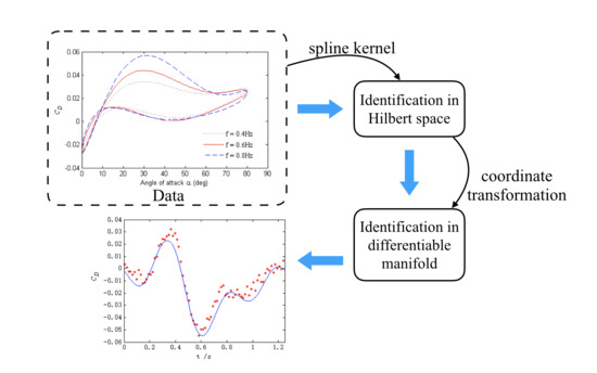
3. Proposed Framework

3.1. Problem Formulation

In recent years, the kernel method has been adopted to construct the basis function. With a defined kernel, $h\left(\mathit{x}\right)$ is represented as

$$h\left(\mathit{x}\right)=\sum _{i=1}^N{\theta }_i{K}_{{\mathit{x}}_i}\left(\mathit{x}\right),$$

(5)

where $K_{{\mathit{x}}_i}(·)$ denotes the kernel function, which can be also described as $K({\mathit{x}}_i,\mathit{x})$.

Based on the definition of the kernel, a Hilbert space $\mathcal{H}$ can be constructed by proving that the Cauchy sequences with the induced norm in the space will converge [31,32]. According to the expected properties for the final model, we set the form for the regularizer $r(·)$ in Equation (3) to be

$$r\left(h\right)={\Vert h\Vert }_{\mathcal{H}}^2=\sqrt{{\langle h,h\rangle }_{\mathcal{H}}},$$

(6)

from which, it can be easily derived that

$$r\left(h\right)=\sum _{i=1}^N\sum _{j=1}^N{\theta }_i{\theta }_{j}K({\mathit{x}}_i,{\mathit{x}}_j).$$

(7)

3.2. Spline Kernel-Based Identification Method

The most widely used kernels include the linear kernels, radial basis kernels, and spline kernels. As is discussed, the regularizer has the form of Equation (6) within the constructed Hilbert space. It is always desired to reduce the impact of noises in identification. There is great significance to design the $r\left(h\right)$ in the form of Equation (4), which penalizes the energy of high-order derivatives. If Equations (4) and (6) can match with each other, the kernel has huge advantages in modeling $h\left(\mathit{x}\right)$. The spline kernel is chosen, because it satisfies the matching relation with the form

$$K({\mathit{x}}_1,{\mathit{x}}_2)={\int }_0^1{G}_p(\Vert {\mathit{x}}_1\Vert ,t)G_p(\Vert {\mathit{x}}_2\Vert ,t)\mathrm{d}t,$$

(8)

where

$$G_p(\Vert \mathit{x}\Vert ,t)=\left\{\begin{array}{cc}\frac{{(\Vert \mathit{x}\Vert -t)}^{p-1}}{(p-1)!}& \mathrm{if}\Vert \mathit{x}\Vert \ge t\\ 0& \mathrm{otherwise}.\end{array}\right.$$

(9)

With the tool of least squares support vector machine method [33], the estimation for $\theta$ is obtained by

$$\hat{\theta }={(\mathit{K}+\gamma I)}^{-1}\mathit{y},$$

(10)

where $\mathit{K}$ is the kernel matrix with ${\mathit{K}}_{ij}=K({\mathit{x}}_i,{\mathit{x}}_j)$, I is an $N\times N$ identity matrix, and $\mathit{y}$ is the output vector with $\mathit{y}={[y_1,y_2,\cdots ,y_N]}^T$.

3.3. Dimensionality Reduction

From Equation (5), we can find that the dimension of state vector $\mathit{x}$, i.e., the number of states, has a huge influence on the model complexity, which also determines the computational complexity of estimation according to Equation (10). However, it is often the case that some states may have little impact on the output of the system because the output has no relationship with the part of states or the information in some states related to the output has already been contained in other states. Consequently, the dimension for the output model can be reduced.

Considering that there exists an intersection among the information of different states, which leads to redundancy in modeling, it is hoped that the information with relevance to the output can be concentrated, and the variables, which provide no additional information on the output except the existing variables, should be abandoned in the modeling process in Equation (5). Coordinate transformation is proposed in this paper, which is discussed in detail in next section. The new state vector is denoted as $\mathit{z}$, with $\mathit{z}\in {\mathbb{R}}^n$. The function realizing the transformation is denoted as $\mathit{z}=t\left(\mathit{x}\right)={[t_1\left(\mathit{x}\right),t_2\left(\mathit{x}\right),\dots ,t_n\left(\mathit{x}\right)]}^T$, where $t_i\left(\mathit{x}\right)$ is a ${\mathbb{R}}^n\to \mathbb{R}$ mapping. $\mathit{z}$ is divided into two part,

$$\mathit{z}={[{\mathit{z}}_1,{\mathit{z}}_2]}^T,$$

(11)

where each of the elements in ${\mathit{z}}_1$ is related with y, while all the elements in ${\mathit{z}}_2$ have no effect on y. Since the definition of the kernel has no dependence on the dimension of the point, the form of the kernel function remains unchanged. The purpose for the transformation is to reduce the dimension of Equation (5)

$$h\left(\mathit{x}\right)=h\left({\mathit{z}}_1\right)$$

(12)

with

$$\sum _{i=1}^N{\theta }_i{K}_{{\mathit{x}}_i}\left(\mathit{x}\right)=\sum _{i=1}^{N^{\prime }}{\beta }_i{K}_{{\mathit{z}}_{1i}}\left({\mathit{z}}_1\right),$$

(13)

where $\beta$ is the parameter vector to be estimated, ${\mathit{z}}_1$ is part of the transformed state vector $\mathit{z}$, $N^{\prime }$ is the number of data for modeling after transformation, and ${\mathit{z}}_1\in {\mathbb{R}}^d$, $d\le n$.

Figure 1 shows the graphical illustration of the proposed framework. It is easy to complete the coordinate transformation for a linear system. However, for a nonlinear system, the transformation is difficult, especially when the transformation is also a nonlinear change.

4. Differential Manifold-Based Transformation

As discussed in the previous section, some of the states in $\mathit{x}$ may present similar information related to y, and some of the states in $\mathit{x}$ may have little impact on y. Aiming at removing the correlation of different states with y, we adopt coordinate transformation to reduce the dimension. Coordinate transformation has been used to obtain more efficient solutions and accelerate the convergence process in optimization problems [34,35]. However, the linear coordinate transformation, which is most widely used, cannot deal with the problem.

We deal with the problem with the tool of differential geometry [36] to obtain nonlinear coordinate transformation. A smooth distribution of dimension $n-d$ is first defined, denoted as $\Delta$, which represents a differentiable manifold. The manifold $\Delta$ is required to be invariant under the vector fields $f,g$, i.e., $f\left(\mathit{x}\right)\in \Delta ,g\left(\mathit{x}\right)\in \Delta$ for all $\mathit{x}$ in $\Delta$. A vector field on $\Delta$ means an assignment of one tangent vector to each $\mathit{x}$ in $\Delta$. f and g can be regarded as mappings from $\Delta$ into the tangent bundles.

To find the transformation $t\left(\mathit{x}\right)$, which is a vector of n real-valued functions of n variables, denoted as

$$\mathit{z}=t\left(\mathit{x}\right)=\left(\begin{array}{c}{t}_1(x_1,x_2,\dots ,x_n)\\ t_2(x_1,x_2,\dots ,x_n)\\ \cdots \\ t_n(x_1,x_2,\dots ,x_n)\end{array}\right),$$

(14)

two assumptions are made:

• The inverse function $t^{\prime }\left(\mathit{z}\right)$ of $t\left(\mathit{x}\right)$ can be found. For any $\mathit{x}$ in $\Delta$, $t^{\prime }\left(t\left(\mathit{x}\right)\right)=\mathit{x}$.
• The functions $t\left(\mathit{x}\right)$ and $t^{\prime }\left(\mathit{z}\right)$ are both continuous and analytic on their domain of definition.

Based on the division of $\mathit{z}$ in Equation (11), we have

$$\frac{\partial h}{\partial z_i}=0,$$

(15)

where $d<i\le n$.

Then, $\Delta$ is contained in the distribution (span{dh})${}^{\perp }$. $\Omega$ is denoted as the orthogonal complement distribution of $\Delta$ with $\Omega ={\Delta }^{\perp }$. For any $\mathit{x}$ in $\Delta$,

$${\Delta }^{\perp }\left(\mathit{x}\right)=\{{\mathit{a}}^{*}\in {\left({\mathbb{R}}^n\right)}^{*}:\langle {\mathit{a}}^{*},\mathit{b}\rangle =0\mathrm{for}\mathrm{all}\mathit{b}\in \Delta \left(\mathit{x}\right)\},$$

(16)

where ${\mathit{a}}^{*}$ is the dual vector and ${\left({\mathbb{R}}^n\right)}^{*}$ is the dual space. If $\mathit{b}$ is a column vector,

$$\mathit{b}=\left[\begin{array}{c}{b}_1\\ b_2\\ \cdots \\ b_n\end{array}\right],$$

(17)

which is a point in $\Delta$, then ${\mathit{a}}^{*}$ is a row vector,

$${\mathit{a}}^{*}=[a_1,a_2,\cdots ,a_n],$$

(18)

which is a point in $\Omega$. The inner product $\langle {\mathit{a}}^{*},\mathit{b}\rangle$ is given by

$$\langle {\mathit{a}}^{*},\mathit{b}\rangle =\sum _{i=1}^n{a}_i{b}_i.$$

(19)

Then, it can be given that $\Omega$ contains the span{dh}, and also is invariant under the vector fields $f,g$.

Aiming at obtaining the maximal dimension reduction of Equation (5), we need to find the smallest distribution which contains $\Omega$ and is invariant under the vector fields $f,g$, denoted by $\langle f,g|\Omega \rangle$. A nondecreasing sequence of distributions is defined

$$\begin{array}{cc}\hfill {\Omega }_0& =\Omega =\mathrm{span}\left\{\mathrm{d}h\right\},\hfill \\ \hfill {\Omega }_1& ={\Omega }_0+[f,{\Omega }_0]+[g,{\Omega }_0]=\mathrm{span}\{\mathrm{d}h,[f,\mathrm{d}h],[g,\mathrm{d}h]\},\hfill \\ \hfill \dots \\ \hfill {\Omega }_k& ={\Omega }_{k-1}+[f,{\Omega }_{k-1}]+[g,{\Omega }_{k-1}].\hfill \end{array}$$

(20)

where $[,]$ is the Lie bracket of vector field, which is an operator to assign a third vector field given two vector fields on a smooth manifold. For any given functions $f_1\left(x\right),f_2\left(x\right)$, the operation $[f_1,f_2]\left(x\right)$ is given by

$$[f_1,f_2]\left(x\right)=\frac{\partial f_2}{\partial x}{f}_1\left(x\right)-\frac{\partial f_1}{\partial x}{f}_2\left(x\right).$$

(21)

According to Lemma 1.9.2 in [36], in iteration process of Equation (20), the equation ${\Omega }_{k^{*}}={\Omega }_{k^{*}+1}$ finally appears for some integer $k^{*}$. Meanwhile, $\langle f,g|\Omega \rangle$ is obtained,

$$\langle f,g|\Omega \rangle ={\Omega }_{k^{*}}.$$

(22)

Finally, we find the real-valued functions ${\mathit{z}}_1\left(\mathit{x}\right)=[t_1\left(\mathit{x}\right),t_2\left(\mathit{x}\right),$$\dots ,t_d{\left(\mathit{x}\right)]}^T$ such that

$$\mathrm{span}\{t_1\left(\mathit{x}\right),t_2\left(\mathit{x}\right),\dots ,t_d\left(\mathit{x}\right)\}={\Omega }_{k^{*}}.$$

(23)

Then, the model of Equation (2) is transformed to

$$\begin{array}{cc}\hfill {\dot{\mathit{z}}}_1& =\tilde{f}\left({\mathit{z}}_1\right)+\tilde{g}\left({\mathit{z}}_1\right)u,\hfill \\ \hfill y& =\tilde{h}\left({\mathit{z}}_1\right),\hfill \end{array}$$

(24)

where

$$\begin{array}{cc}\hfill \tilde{f}\left(\mathit{z}\right)& ={\left[\frac{\partial t}{\partial \mathit{x}}f\left(\mathit{x}\right)\right]}_{\mathit{x}=t^{\prime }\left(\mathit{z}\right)},\hfill \\ \hfill \tilde{g}\left(\mathit{z}\right)& ={\left[\frac{\partial t}{\partial \mathit{x}}g\left(\mathit{x}\right)\right]}_{\mathit{x}=t^{\prime }\left(\mathit{z}\right)},\hfill \\ \hfill \tilde{h}\left(\mathit{z}\right)& ={\left[h\left(\mathit{x}\right)\right]}_{\mathit{x}=t^{\prime }\left(\mathit{z}\right)}.\hfill \end{array}$$

(25)

Compared with the original description, the dimension of the new description is reduced. The number of data required for accurate identification is reduced, which corresponds to $N^{\prime }$ in Equation (13). Consequently, the number of parameters to be estimated is highly reduced.

5. Simulation and Evaluation

In this section, the proposed identification approach is evaluated and compared with the commonly used methods. A brief introduction to the experimental settings is first given. Comparison of the evaluation results with other methods is then made.

5.1. Background Information

To validate the proposed method for nonlinear systems, aerodynamic coefficients at large angles of attack were considered, which present significant nonlinear phenomena in the wind tunnel experiments. With the FL-8 wind tunnel, large amplitude forced oscillation tests were made. The model to be tested was chosen to be the fourth-generation fighter configuration [37].

Table 1. Physical parameters of the experimental prototype.

Physical Parameter	Value
Weight	≤8 kg
Length	1.1825 m
Wing Span	0.8475
Wing Area	0.3047 m${}^2$
Mean Aerodynamic Chord	0.4269 m
Position of Aerodynamic Center	0.6926 m

gives the main physical parameters for the experimental model. In the tests, the flow speed was 30 m/s. The sampling period was 0.02 s.

The state vector for aerodynamic identification was constructed by

$$\mathit{x}=[\alpha ,\dot{\alpha },\ddot{\alpha },q,\dot{q},{\delta }_e,M]$$

(26)

where $\alpha$ is the angle of attack, q is the pitch rate, ${\delta }_e$ is the elevator control surface deflection, and M is the Mach number.

The state equation for $x_1\left(k\right)=\alpha \left(k\right),x_2\left(k\right)=\dot{\alpha \left(k\right)},x_3\left(k\right)=\ddot{\alpha }$ can be given by

$$\left[\begin{array}{c}{x}_1\left(k\right)\\ x_2\left(k\right)\\ x_3\left(k\right)\end{array}\right]=\left[\begin{array}{ccc}1& \Delta t& \Delta t^2/2\\ 0& 1& \Delta t\\ 0& 0& 1\end{array}\right]\left[\begin{array}{c}{x}_1(k-1)\\ x_2(k-1)\\ x_3(k-1)\end{array}\right]+\left[\begin{array}{c}{w}_1(k-1)\\ w_2(k-1)\\ w_3(k-1)\end{array}\right].$$

(27)

where $\Delta t$ denotes the time period of the measurements, and $w\left(k\right)$ is the state noise.

Corresponding to the form of Equation (2), the first three elements of $f\left(\mathit{x}\right)$ and $g\left(\mathit{x}\right)$ are linear. The construction for the remaining part of $f\left(\mathit{x}\right)$ and $g\left(\mathit{x}\right)$ can be obtained according to the physical mechanism, e.g., through table interpolation.

5.2. Comparison Results and Discussions

The nonlinear aerodynamic coefficients in the large amplitude pitch oscillation tests for three frequencies are shown in Figure 2. The test is conducted at the balanced angle of 40${}^{\circ }$ with amplitude of 40${}^{\circ }$, and the sideslip angle is −30${}^{\circ }$.

When the test data are not sufficient, the data-driven models including step response model and neural networks cannot be identified. We compared the proposed identification approach with the standard spline kernel-based method. We chose the experimental condition with frequency of 0.8 Hz. The estimation results are shown in Figure 3. In terms of the lift coefficient with slow time-varying characteristics, the proposed approach and the standard spline kernel method demonstrate almost the same tracking ability. The improvement is not obvious because of the locally linear features in the curve. In terms of the drag coefficient, which contains more complex nonlinear characteristics, the performance of the proposed method is obviously better. Given the same amount of training data, more features are caught by the proposed approach. The comparison results of objective function with the form of Equation (3) is given in

Table 2. Comparison results of values of objective function in Equation (3).

Algorithm	${\mathit{C}}_{\mathit{L}}$	${\mathit{C}}_{\mathit{D}}$
The Proposed Approach	1.2996	0.0032
The Standard Kernel Method	1.6458	0.0102

, which proves that the proposed algorithm can track the hysteresis with a higher accuracy. As discussed above, in addition to the accuracy, the construction of Equation (3) also takes into account of the generalization ability of the model. Therefore, the proposed method has better generalization ability and is less sensitive to the noises in observations.

Additionally, with the strategy of dimensionality reduction, the new state vector $\mathit{z}$ transformed from $\mathit{x}$ is divided into ${\mathit{z}}_1$ and ${\mathit{z}}_2$. The dimension of the state vector ${\mathit{z}}_1$ finally input to the spline kernel-based model is 3. Therefore, the dimension of the final output model $h\left({\mathit{z}}_1\right)$ is 3. Compared with the standard spline kernel-based model, the proposed approach constructs a model with fewer parameters. Estimation is made with lower computational cost, while the information in the data is used more efficiently.

6. Conclusions

In this work, a novel spine kernel-based approach with dimensionality reduction is designed for nonlinear system identification. A regularization term based on the produced Hilbert space is added into the objective function to guarantee the generalization ability of the model. Dimensionality reduction is proposed to solve the problem of kernel methods when applied to data with high dimensions. By reducing the dimension of the state vector, the number of parameters in the estimation is significantly reduced. With the tool of Lie bracket, nonlinear coordinate transformation is made based on the defined distribution of the differentiable manifold. Clear physical meaning is given that the transformation concentrates the information on the states related to the output, and abandons the redundant states. After the transformation, the new state vector reduces the dimensions of the new description. Evaluation on the nonlinear aerodynamic coefficients under the wind tunnel tests was made. The experimental results show that the proposed method successfully approximates the data in the nonlinear system and achieves higher accuracy and better generalization ability through dimensionality reduction. The future work will include analyzing the effects of the regularization parameter $\gamma$ on the performance of the identification method, and subsequently linking the estimation of $\gamma$ into the identification framework.

References

1. Zhu, M.; Feng, Z.; Zhou, X.; Xiao, R.; Qi, Y.; Zhang, X. Specific emitter identification based on synchrosqueezing transform for civil radar. Electronics 2020, 9, 658. [Google Scholar] [CrossRef]
2. Guo, M.; Su, Y.; Gu, D. System identification of the quadrotor with inner loop stabilisation system. Int. J. Model. Identif. Control 2017, 28, 245–255. [Google Scholar] [CrossRef]
3. Moreno, R.; Moreno-Salinas, D.; Aranda, J. Black-box marine vehicle identification with regression techniques for random manoeuvres. Electronics 2019, 8, 492. [Google Scholar] [CrossRef] [Green Version]
4. Baldini, A.; Ciabattoni, L.; Felicetti, R.; Ferracuti, F.; Freddi, A.; Monteriù, A. Dynamic surface fault tolerant control for underwater remotely operated vehicles. ISA Trans. 2018, 78, 10–20. [Google Scholar] [CrossRef]
5. He, W.; Ge, W.; Li, Y.; Liu, Y.J.; Yang, C.; Sun, C. Model identification and control design for a humanoid robot. IEEE Trans. Syst. Man Cybern. Syst. 2016, 47, 45–57. [Google Scholar] [CrossRef] [Green Version]
6. Veksler, A.; Johansen, T.A.; Borrelli, F.; Realfsen, B. Dynamic positioning with model predictive control. IEEE Trans. Control. Syst. Technol. 2016, 24, 1340–1353. [Google Scholar] [CrossRef] [Green Version]
7. Haidegger, T.; Kovács, L.; Preitl, S.; Precup, R.E.; Benyo, B.; Benyó, Z. Controller design solutions for long distance telesurgical applications. Int. J. Artif. Intell. 2011, 6, 48–71. [Google Scholar]
8. Ljung, L.; Wahlberg, B. Asymptotic properties of the least-squares method for estimating transfer functions and disturbance spectra. Adv. Appl. Probab. 1992, 24, 412–440. [Google Scholar] [CrossRef]
9. Yang, C.; Jiang, Y.; He, W.; Na, J.; Li, Z.; Xu, B. Adaptive parameter estimation and control design for robot manipulators with finite-time convergence. IEEE Trans. Ind. Electron. 2018, 65, 8112–8123. [Google Scholar] [CrossRef]
10. Jasim, W.; Gu, D. Robust path tracking control for quadrotors with experimental validation. Int. J. Model. Identif. Control 2018, 29, 1–13. [Google Scholar] [CrossRef]
11. Pillonetto, G.; De Nicolao, G. Pitfalls of the parametric approaches exploiting cross-validation for model order selection. IFAC Proc. Vol. 2012, 45, 215–220. [Google Scholar] [CrossRef]
12. Fanesi, M.; Scaradozzi, D. Adaptive control for non-linear test bench dynamometer systems. In Proceedings of the 2019 IEEE 23rd International Conference on System Theory, Control and Computing (ICSTCC), Sinaia, Romania, 9–11 October 2019; pp. 768–773. [Google Scholar]
13. Sun, J.; Yang, Q. Research on least means squares adaptive control for automotive active suspension. In Proceedings of the 2008 IEEE International Conference on Industrial Technology, Chengdu, China, 21–24 April 2008; pp. 1–4. [Google Scholar]
14. Yang, E.; Gu, D.; Hu, H. Performance improvement for formation-keeping control using a neural network HJI approach. In Trends in Neural Computation; Springer: Berlin, Germany, 2007; pp. 419–442. [Google Scholar]
15. He, W.; Yan, Z.; Sun, Y.; Ou, Y.; Sun, C. Neural-learning-based control for a constrained robotic manipulator with flexible joints. IEEE Trans. Neural Netw. Learn. Syst. 2018, 29, 5993–6003. [Google Scholar] [CrossRef] [PubMed]
16. Zhang, Z.; Jiang, T.; Li, S.; Yang, Y. Automated feature learning for nonlinear process monitoring—An approach using stacked denoising autoencoder and k-nearest neighbor rule. J. Process. Control 2018, 64, 49–61. [Google Scholar] [CrossRef]
17. Zhou, X.; Jiang, P.; Wang, X. Recognition of control chart patterns using fuzzy SVM with a hybrid kernel function. J. Intell. Manuf. 2018, 29, 51–67. [Google Scholar] [CrossRef]
18. Ai, Q.; Wang, A.; Zhang, A.; Wang, W.; Wang, Y. An effective multiclass twin hypersphere support vector machine and its practical engineering applications. Electronics 2019, 8, 1195. [Google Scholar] [CrossRef] [Green Version]
19. Chodunaj, M.; Szcześniak, P.; Kaniewski, J. Mathematical modeling of current source matrix converter with Venturini and SVM. Electronics 2020, 9, 558. [Google Scholar] [CrossRef] [Green Version]
20. Pillonetto, G.; De Nicolao, G. A new kernel-based approach for linear system identification. Automatica 2010, 46, 81–93. [Google Scholar] [CrossRef]
21. Han, T.; Wang, L.; Wen, B. The kernel based multiple instances learning algorithm for object tracking. Electronics 2018, 7, 97. [Google Scholar] [CrossRef] [Green Version]
22. Pillonetto, G.; Dinuzzo, F.; Chen, T.; De Nicolao, G.; Ljung, L. Kernel methods in system identification, machine learning and function estimation: A survey. Automatica 2014, 50, 657–682. [Google Scholar] [CrossRef] [Green Version]
23. Chen, T. Continuous-time DC kernel-a stable generalized first-order spline kernel. IEEE Trans. Autom. Control 2018, 63, 4442–4447. [Google Scholar] [CrossRef] [Green Version]
24. Dreano, D.; Tandeo, P.; Pulido, M.; Ait-El-Fquih, B.; Chonavel, T.; Hoteit, I. Estimating model-error covariances in nonlinear state-space models using Kalman smoothing and the expectation—Maximization algorithm. Q. J. R. Meteorol. Soc. 2017, 143, 1877–1885. [Google Scholar] [CrossRef] [Green Version]
25. Zhang, J.X.; Yang, G.H. Prescribed performance fault-tolerant control of uncertain nonlinear systems with unknown control directions. IEEE Trans. Autom. Control 2017, 62, 6529–6535. [Google Scholar] [CrossRef]
26. Zhang, K.; Zhang, H.; Xiao, G.; Su, H. Tracking control optimization scheme of continuous-time nonlinear system via online single network adaptive critic design method. Neurocomputing 2017, 251, 127–135. [Google Scholar] [CrossRef]
27. Ding, F.; Xu, L.; Alsaadi, F.E.; Hayat, T. Iterative parameter identification for pseudo-linear systems with ARMA noise using the filtering technique. IET Control Theory Appl. 2018, 12, 892–899. [Google Scholar] [CrossRef]
28. Esfahani, A.F.; Dreesen, P.; Tiels, K.; Noël, J.P.; Schoukens, J. Parameter reduction in nonlinear state-space identification of hysteresis. Mech. Syst. Signal Process. 2018, 104, 884–895. [Google Scholar] [CrossRef]
29. Zanotti, C.; Rotiroti, M.; Sterlacchini, S.; Cappellini, G.; Fumagalli, L.; Stefania, G.A.; Nannucci, M.S.; Leoni, B.; Bonomi, T. Choosing between linear and nonlinear models and avoiding overfitting for short and long term groundwater level forecasting in a linear system. J. Hydrol. 2019, 578, 124015. [Google Scholar] [CrossRef]
30. Schaefer, I.; Kosloff, R. Optimization of high-order harmonic generation by optimal control theory: Ascending a functional landscape in extreme conditions. Phys. Rev. A 2020, 101, 023407. [Google Scholar] [CrossRef] [Green Version]
31. Mu, B.; Chen, T.; Ljung, L. On asymptotic properties of hyperparameter estimators for kernel-based regularization methods. Automatica 2018, 94, 381–395. [Google Scholar] [CrossRef] [Green Version]
32. Steinwart, I.; Hush, D.; Scovel, C. An explicit description of the reproducing kernel Hilbert spaces of Gaussian RBF kernels. IEEE Trans. Inf. Theory 2006, 52, 4635–4643. [Google Scholar] [CrossRef]
33. Suykens, J.A.K.; Vandewalle, J. Least squares support vector machine classifiers. Neural Process. Lett. 1999, 9, 293–300. [Google Scholar] [CrossRef]
34. Fang, W.; Zhang, L.; Yang, S.; Sun, J.; Wu, X. A multiobjective evolutionary algorithm based on coordinate transformation. IEEE Trans. Cybern. 2019, 49, 2732–2743. [Google Scholar] [CrossRef] [PubMed] [Green Version]
35. Yu, Z.; Qin, M.; Chen, X.; Meng, L.; Huang, Q.; Fu, C. Computationally efficient coordinate transformation for field-oriented control using phase shift of linear hall-effect sensor Signals. IEEE Trans. Ind. Electron. 2019, 67. [Google Scholar] [CrossRef]
36. Isidori, A. Nonlinear Control Systems; Springer Science & Business Media: Berlin, Germany, 2013. [Google Scholar]
37. Liu, C.; Zhao, Z.; Bu, C.; Wang, J.; Mu, W. Double degree-of-freedom large amplitude oscillation test technology in low speed wind tunnel. Acta Aeronaut. Astronaut. Sin. 2016, 37, 2417–2425. [Google Scholar]
Figure 1. Graphical illustration of the proposed framework.
Electronics 09 00940 g001
Figure 2. Example of longitudinal oscillations: (a) lift coefficients C L for 0.4, 0.6, and 0.8 Hz; and (b) Drag coefficients C D for 0.4, 0.6, and 0.8 Hz.
Electronics 09 00940 g002
Figure 3. Real-time estimation results of the longitudinal oscillation, where the dotted line shows the real values from the wind tunnel test and the solid line is the estimation result: (a) Lift coefficients C L with the proposed approach; (b) lift coefficients C L with the standard spline kernel method; (c) drag coefficients C D with the proposed approach; and (d) drag coefficients C D with the standard spline kernel method.
Electronics 09 00940 g003