A Mobile Augmented Reality System for the Real-Time Visualization of Pipes in Point Cloud Data with a Depth Sensor

Abstract

Augmented reality (AR) is a useful visualization technology that displays information by adding virtual images to the real world. In AR systems that require three-dimensional information, point cloud data is easy to use after real-time acquisition, however, it is difficult to measure and visualize real-time objects due to the large amount of data and a matching process. In this paper we explored a method of estimating pipes from point cloud data and visualizing them in real-time through augmented reality devices. In general, pipe estimation in a point cloud uses a Hough transform and is performed through a preprocessing process, such as noise filtering, normal estimation, or segmentation. However, there is a disadvantage in that the execution time is slow due to a large amount of computation. Therefore, for the real-time visualization in augmented reality devices, the fast cylinder matching method using random sample consensus (RANSAC) is required. In this paper, we proposed parallel processing, multiple frames, adjustable scale, and error correction for real-time visualization. The real-time visualization method through the augmented reality device obtained a depth image from the sensor and configured a uniform point cloud using a voxel grid algorithm. The constructed data was analyzed according to the fast cylinder matching method using RANSAC. The real-time visualization method through augmented reality devices is expected to be used to identify problems, such as the sagging of pipes, through real-time measurements at plant sites due to the spread of various AR devices.

1. Introduction

A point cloud is typically a collection of data taken from an object using a laser scanner. This measured data is used in various fields, such as autonomous driving, space reconstruction, 3D printing, drones, robotics, and digital twins. Point clouds are often used for the purpose of measuring and quality inspection of manufactured parts and generating 3D CAD models. This is called reverse engineering. Reverse engineering is a design process that analyzes or reproduces a product from a physical part. It is useful in modeling tasks to experiment, evaluate, and verify conceptual designs for new product designs. Of these, reverse engineering of plant facilities is in increasing demand.

Reverse engineering of plant facilities is used for factory relocation, modernization, capacity expansion, and efficiency improvements of already built and operating facilities. Reverse engineering can make drawings easier to maintain, such as through part interference. Simulations using virtual space, such as virtual maintenance and simulation training using reverse engineering, are utilized in various areas [1].

To reverse engineer of a plant facility, workers first install laser scanners in various locations to acquire point data. The measured data is integrated into the same coordinate system through the registration process, and then manually constructed as building information modeling (BIM) data. In general, the plant facilities are so large that the measured point cloud data is also very large. Therefore, manual works for constructing BIM data require a great deal of manpower and time. To reduce these shortcomings, many studies on modeling automation in point clouds have been conducted. The automatic pipe estimation algorithm, which is a large aspect of plant facilities, can reduce the opportunity cost of manual labor.

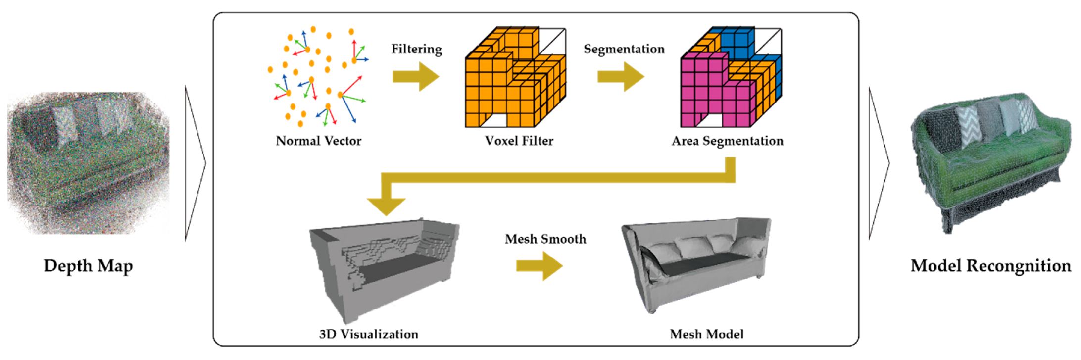
Pipes, which account for a large proportion of the reverse engineering of plant facilities, are relatively easy to automate and much research has been done with them. In general, the automatic estimation of pipes is accomplished through normal estimation, segmentation, and filtering, as shown in Figure 1.

Normal estimation is a process of estimating the normal of a face when each point in a set of points forms a face, and filtering is a process of removing the noise based on the calculated normals. Segmentation is the process of grouping a set of points that form the same object around the normals from the noise-free data, and model estimation is the process of estimating the shape of the object based on each segmented group.

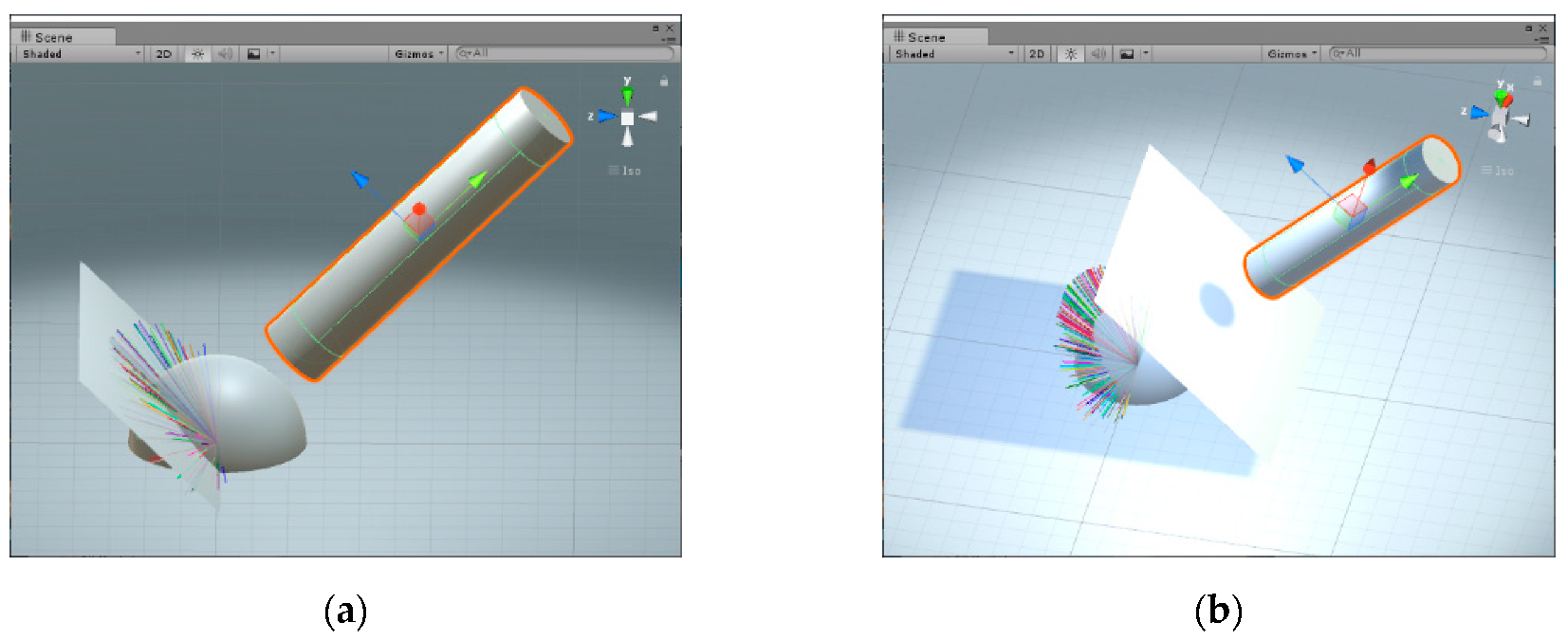
When the preprocessing process is completed, the pipe is selected from each of the recognized objects to determine the length and diameter, and the pipe modeling is completed. In this case, the Hough transform is generally used. The Hough transform determines the direction of the pipe by voting after arranging the normals of the points formed by the pipes around the Gaussian sphere. (a) of Figure 2 illustrates this process.

Once the direction of the pipe is determined, the pipe modeling is completed by assuming that the circle formed by orthogonalizing each point of the pipe on a plane having the same normal as the direction of the pipe and the diameter of the pipe as shown in Figure 2b [2,3,4,5,6,7,8].

Existing methods perform the segmentation process after normal estimation; therefore, accurate normal estimation is very important. Recently, the accuracy of the laser sensors has been improved greatly, and the error of the point data is very small. Mobile augmented reality devices (including stand-alone devices, such as Facebook Smartglasses and MS HoloLens), however, operate at low power and are relatively weak in accuracy. Therefore, we need to compensate for the shortcomings of mobile augmented reality devices by using a fast pipe estimation algorithm without normal estimation.

In the point cloud, the estimation of pipes without normal estimation includes methods using sphere fitting and principal component analysis. The procedure of the above method calculates the parameters through mathematical modeling of spheres and straight lines. In this case, a noise reduction method using random sample consensus (RANSAC) is used. By defining the parameters that fit the model of the defined sphere, we can construct a central axis candidate group (center point and radius). The central axis candidate group also becomes a point cloud and estimates the central axis of the pipe from the central axis candidate group using the length and radius averages of the regions corresponding to the linear model. This method is relatively fast and does not require normal estimation, making it suitable for mobile augmented reality devices. Therefore, this paper presents the possibility of real-time pipe estimation using mobile augmented reality devices based on the above method.

Augmented reality is a field of virtual reality (VR) involving a computer graphics technique that synthesizes virtual objects in the real environment to make the real and virtual appear together. Recently, with the development of augmented reality devices, wearable devices of low power have been released and applied in various fields. For example, distance information using a smartphone’s camera, additional clarifications in education, additional information needed for flight, and model visualization during building project meetings. In addition, the application of augmented reality (AR)/VR is exploding [9,10,11,12].

Various studies using point cloud data and augmented reality devices have been conducted. Gupta developed a method using LiDAR data to solve the problem of augmenting dimensional information for mobile augmented reality system [13]. Placitelli developed a face alignment tool that can be applied to real-time video streams using RGB and depth images [14]. Gao developed an AR framework for accurate and stable virtual object matching for realistic tracking and recognition [15]. Mancera-Taboada built augmented and virtual reality-based platforms that provide digital access for the disabled using 2D technical drawings (ground plan, front elevation, and sectional view), laser scanners, and digital cameras [16]. Schwarz proposed a real-time augmented reality technology in mobile devices through compression technology based on an mpeg video-based point cloud [17].

Mahmood proposed a RANSAC-based false correspondence rejection method to increase the accuracy in registration and correspondence estimation required for interaction in augmented reality devices [18]. Kung extracted planar and curved regions using supervoxel segmentation for AR devices [19]. Pavez studied the compression and expression of the polygon cloud, which is the middle between the polygon mesh and the point cloud on the AR device. A dynamic polygonal cloud has the advantage of temporal redundancy for compression; thereby, they proposed compressing static/dynamic multiple clouds [20]. Cazamias used depth images for the real-time processing of technology to create virtual spaces based on real spaces [21].

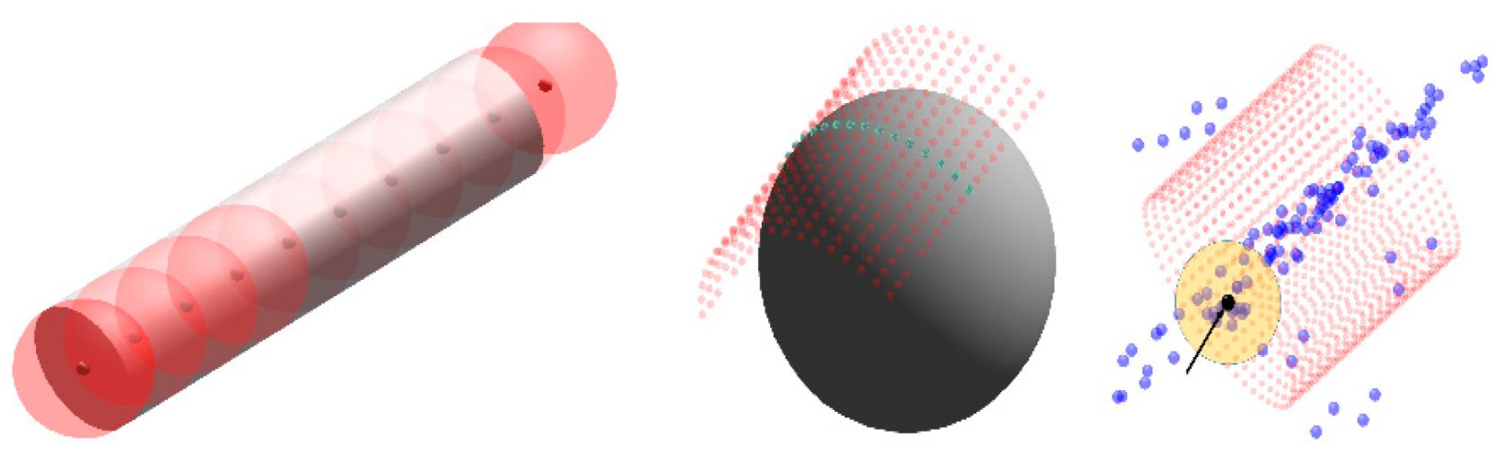
Jimeno-Morenilla proposed real-time footwear matching using a glove system that can control a 3D model and a magic mirror. In particular, the infrared emission sensor was attached to the foot to measure the position and direction, and the 3D shoe was augmented to complete the magic mirror [22]. Based on the above research, after a real-time pipe measurement using a point cloud, the augmented reality visualization method first acquires a point cloud from a depth image and downscales it as shown in Figure 3. After that, the center axis estimation using the variable scale is performed for the pipe estimation. After estimating the exact pipe by accumulating the estimated results, the augmented reality is constructed/completed by integrating the actual image and the estimated object.

In the remainder in the article, Section 2 deals with the pipe estimation methodology, and Section 3 contains the Experimental Results and Discussion. Finally, Section 4 presents our conclusions.

2. Materials and Methods

2.1. Pipe Estimation

To estimate the cylindrical object in the point cloud, this paper uses RANSAC. RANSAC is a methodology [23,24] that takes samples repeatedly from given data and analyzes the entire dataset. As this method uses only some data, it is relatively fast and noise-resistant. RANSAC also consumes less resources than the Hough transform, so its value is high. RANSAC fitting requires the definition of mathematical models of a sphere and straight line.

Figure 4 shows that a sphere with the same diameter as the cylinder leaves a trace of the sphere’s center point while moving along the inside of the cylinder. As shown in the figure, the center and radius of the sphere is calculated by the sphere fitting through neighbors around a point in the point cloud.

The radius and center point of the sphere can be calculated by defining a mathematical model. A set of traces using spheres can be used to estimate the direction, which can be assumed to be the central axis of the cylinder. Therefore, a straight line must be modeled to estimate the central axis. At this time, principal component analysis is used to model the straight line. Principal component analysis (PCA) is a statistical approach to estimate the directions e2 and e3, which are perpendicular to the directions e1 with the largest variance of data as shown in Figure 5 [25,26]. Therefore, when e1 is found, the direction of the cylinder central axis can be known. Principal component analysis constructs a covariance matrix and obtains a direction vector by eigen-decomposition of the covariance matrix.

Figure 6 depicts the estimate of the central axis, where Figure 6a is the result of calculating the eigenvectors based on the neighboring points at one point, and Figure 6b is the sum of the eigenvectors. This is the result of estimating the direction and length. At this point, the constant criterion is the distance and angle of the two vectors. In other words, if the angle and distance formed by the two vectors are within a certain range, then they are considered as one vector. At this time, the radius average of the central axis candidate group that constitutes one vector becomes the radius of the cylinder. Figure 6c is a result of matching a straight line through the sum of the blue eigenvectors.

The above method can also be used to estimate pipe elbows, as shown in Figure 7. For more information on fast cylinder estimation in point clouds, please see [27].

2.2. Real-Time Visualization

2.2.1. Data Parallelism

When using a single core in a point cloud, the tasks are performed sequentially. For example, the method of Section 2.1 receives the point data, structures the data with K-Dimension Tree (KDTree), and then estimates the cylinder area through the central axis estimation. KDTree is a structured algorithm that allows quick access to each point in the point data. Parallel processing of time-consuming work (center axis estimation) in this series of processes can theoretically improve the performance by the number of cores.

Multiple cores are central processing unit (CPU)s that have two or more cores in a single integrated circuit and share memory in each core. However, in the operating system (OS), performance may degrade when different threads access the same memory area at the same time. Therefore, for parallel processing using multiple threads, KDTree data must be secured in the memory area for the parallel processing as shown in Figure 8. In other words, in the proposed method, parallel processing using a CPU should construct as many KDTree data structures as the number of cores used. Therefore, as shown in Figure 8b, there is no choice but to use as much memory as the number of cores.

If four cores are used for parallel processing, the memory is used four times as compared to a single core as shown in Figure 8b. However, each thread does not use the entire memory, but only uses a portion (red box) of it. Such processing can improve speed; however, memory waste is inevitable. One way to reduce memory waste is to retrieve a region of data of interest and load it into the memory. However, because there is an opportunity cost of searching for the area of interest data, this is not covered.

Figure 9 shows parallel processing of the sphere fitting. Each core estimates the central axis candidates from a limited area of data (memory) and, when all cores are done, integrates the results to complete the estimation of the central axis candidates. In other words, each core estimates the candidate group for the central axis from the data belonging to the red box in Figure 8b, and the estimated results are integrated into one as shown in Figure 9b to complete the estimation for the central axis candidate group.

Parallel processing not only shortens the execution time but can also be used for accuracy. The method in Section 2.1 finds solutions using a local approach. Therefore, in parallel processing, the whole area is divided by a certain ratio and the results are integrated to find a cylinder. In this case, if each core is responsible for the entire region without dividing the entire region by a certain ratio, the result of the central axis estimation will be expected to be more sophisticated. Alternatively, if the center axis estimation is performed first and then the center axis estimation is performed on each core based on the result, the accuracy can be increased while reducing the execution time.

As described above, the method of Section 2.1 has a simple structure that simply divides the domain without any additional work for parallel processing. Therefore, the parallel processing can be applied in various ways, so that the cylinder can be estimated quickly and accurately.

2.2.2. Real-time Estimation Using Depth Image

In Figure 3, depth images are used for real-time cylinder estimation and visualization. The depth image is an image that provides a distance value for each pixel. Point clouds can be constructed by sampling pixels at regular intervals in this image. The Kinect (MS, Redmond, WA, USA) is well known as a device for inexpensively and easily obtaining depth images.

Kinect V1 can generate 30 frames per second of 640 × 480 resolution depth image using structured light (an infrared sensor). By constructing a point cloud by sampling 20–50% of the image generated from Kinect, and down sampling with the voxel grid method, a point cloud with a uniform distribution can be completed as shown in Figure 10.

Once a uniform point cloud is complete, real-time cylinder estimation is possible. However, the cylinder estimation using the data obtained in one aspect is inevitably lowered. Therefore, rather than estimating cylinders for each frame, estimating cylinders by incorporating several frames with sphere fitting is one way to increase accuracy. Figure 11 depicts this process.

Figure 11a shows the results of the central axis estimation from the point data acquired in each frame, and Figure 11b shows the results of accumulating and filtering the results of Figure 11a.

As shown in Figure 11, real-time cylinder estimation acquires a point cloud from a depth image and voxelizes the data by down sampling from the acquired data. When sphere fitting is performed on the uniformized data, one frame is completed, and cylinder matching is performed after filtering the accumulated data for three to four frames.

Matching through frame accumulation is easier to filter as the amount of central axis candidate data is smaller in this region except for the cylinder region. In other words, there are more central axis candidate data in the cylinder region. Therefore, when the central axis candidate data is less than or equal to the threshold, it can be regarded as noise, thereby minimizing the noise. However, there is inevitably a disadvantage in the execution time compared with the single frame matching.

Depth images generally also have the disadvantage of being less accurate over long distances. Therefore, they are suitable for the estimation of cylinders at a close distance. As a result, if the diameter of the cylinder is large, the depth image cannot be acquired in one screen, and thus a small pipe should be targeted. In point data, the smaller diameter cylinder has a smaller curved surface, which increases the area where sphere fitting does not work. To overcome this problem, the scale of the point data obtained from the depth image must be processed k times, and then 1/k reciprocal times again after the processing in Section 2.1.

Figure 12a shows the result of using the scale of the data obtained from the depth image as it is, and Figure 12b shows the result of matching after expanding the scale of the point data by five times. In Figure 12b, unlike Figure 12a, the cylinder was estimated.

3. Results and Discussions

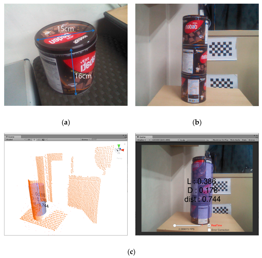
3.1. Cylinder Estimation Using Kinect V1

Real-time estimation of the depth images in Section 2.2 used Kinect V1 and RealSense SR300. The data is composed as shown in Figure 13b by sampling about 15% from the depth image with a 640 × 480 resolution.

As shown in Figure 13a, the cylinders used for the experiment were constructed using three cans of 15 cm in diameter and 16 cm in length as shown in Figure 13b. For the constructed data, the single frame cylinder estimation is shown in Figure 13c. The experiments used Unity3D on laptops equipped with an Intel 8250U CPU operating at 3.40 GHz and 16 GB memory.

Figure 13c shows the result of estimating the central axis every frame. This handles the average filter but is noisy, the matching results are inaccurate, and the results showed 2.08 frames per second. In addition, some frame estimation is impossible, and the estimation results are inconsistent. Based on these results, there was an error of about 15% in the diameter (15 cm). The result corrected using this ratio is shown in Figure 13d. The data obtained from the depth image has an error rate depending on the distance. Therefore, the error according to the distance must be corrected.

Figure 14 shows the error result over distance. At a 60 cm distance from the camera, the error in the diameter was close to zero, and the error was the greatest at 95 cm. This shows that the error increased linearly. Therefore, the diameter error can be easily corrected.

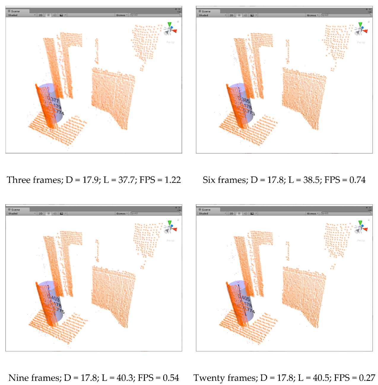
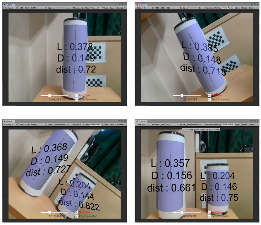
A single frame produces inconsistent estimates. Increasing the value of ϵ (sampling rate) gives a better estimate, but using multiple frames yields better estimates.

Figure 15 shows that the multi-frame center axis estimates with better accuracy and consistency than a single frame. However, as the number of integrated frames increases, the number of frames per second decreases.

The real-time cylinder estimation method generated uniform data based on one surface in the depth image. The accuracy was inevitably lower than that of the registered data, as the straight line region was estimated after the sphere fitting and central axis candidate data integration. To overcome this, distance correction and multi-frames can improve the consistency and accuracy; however, this takes a long time to execute. This problem of processing speed may be solved through parallel processing. 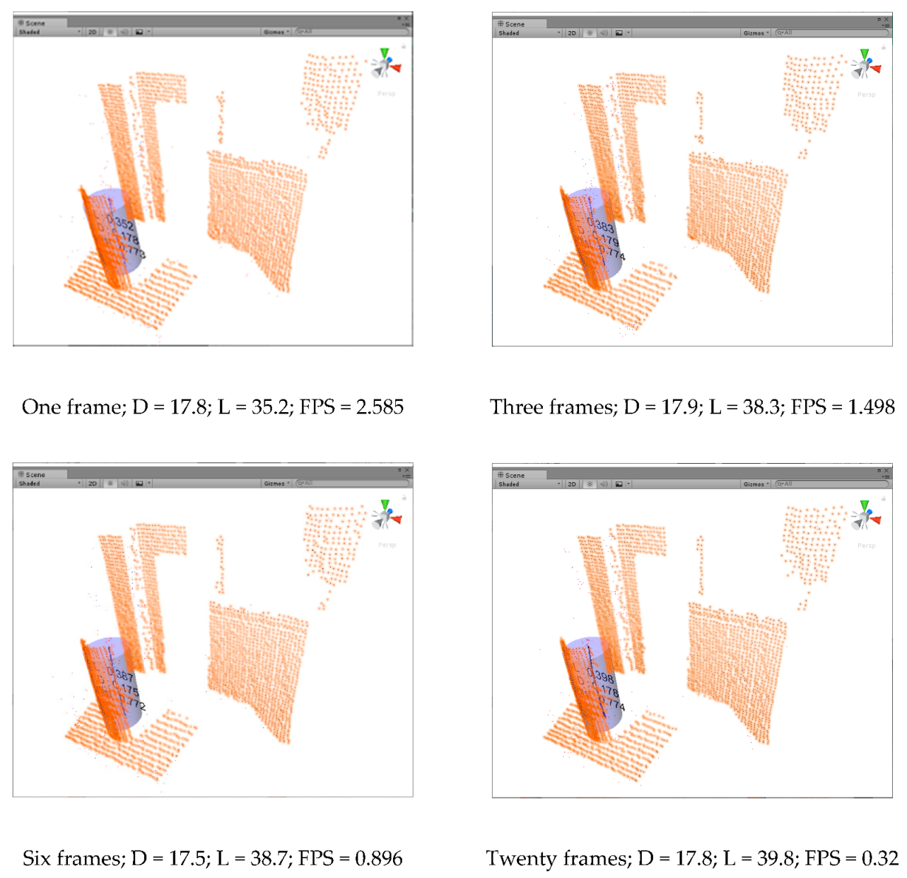Figure 16 shows the performance improvement through parallel processing in real-time cylinder estimation.

Parallel processing resulted in improved frame rates in the real-time estimation, but there was no significant difference in the accuracy. However, matching consistency showed a better appearance, which we estimate as a result of overlapping calculations in the divided regions for the sphere fit.

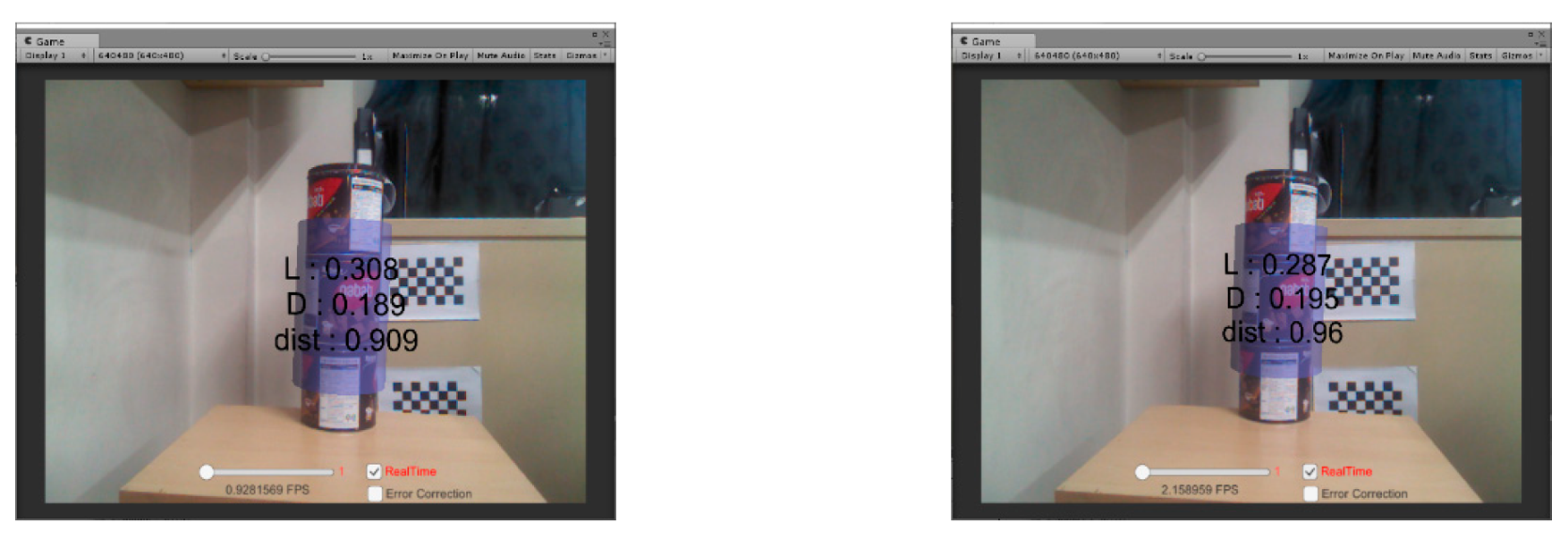
Finally, real-time cylinder estimation was completed when the estimated cylinder corresponded to the RGB image. Figure 17 shows the result of mapping the estimated cylinder to an RGB image. Kinect’s actual RGB image FOV was 62° × 48.6°. Unity3D’s camera FOV can be set to 48.6° to correspond to the actual video. However, accurate pipe estimation is not possible and due to problems such as camera distortion, an accurate 1:1 correspondence is not shown.

In Figure 17, the two pipes also match and when the camera is tilted and measured assuming a pipe installed diagonally, it can be estimated. However, error correction was applied because the matching result was not good.

Kinect V1 is a device with a phase-shift method that has been in use for years. As the measurement data is inaccurate and rather slow, we attempted to measure/compare the same model using Intel’s RealSense SR300 sensor.

3.2. Cylinder Estimation Using SR300

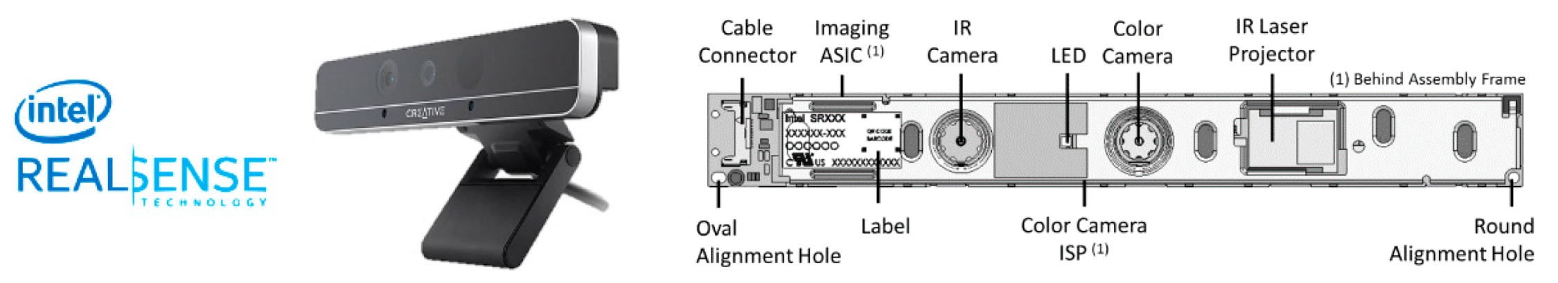
The SR300 (Intel, Santa Clara, CA, USA) was launched in 2016 and is a coded light sensor. The measurement range is 0.3 m to 2 m and the depth resolution is VGA 30FPS. Figure 18 shows the internal structure of the SR300, which uses infrared (IR) and RGB cameras to estimate the depth, with on-demand integrated circuits for image processing. The FOV is 68° × 41.5°.

Figure 19a shows the characteristics of the SR300 sensor. The distance is calculated by measuring the pattern when the light emitted from the IR sensor is reflected. In Figure 19a is the result of reflecting only a part of the entire surface due to diffuse reflections. To solve this problem, the surface was treated to prevent diffuse reflections as shown in Figure 19b.

Figure 20 shows the measurement results using SR300, a coded light sensor. Compared to Kinect, which is a phase modulation method (structured light), the overall result was up to two frames or more, and the response speed was relatively good; however, the accuracy was insufficient. This is presumed to be the result of a lack of surface treatment.

In general, coded light sensors have advantages in miniaturization and accurate operation, and can be mass-produced by semiconductor processes. In addition, the sensor can generate dense, high-resolution codes using a continuous pattern. However, this sensor has a disadvantage in that the temporal consistency of the constructed code can be broken when an object moves in the scene. The SR300 has overcome this shortcoming in the short range by using a fast video graphics array (VGA) infrared camera and a 2-M pixel RGB color camera with an integrated image signal processor [28,29].

3.3. Real-Time Pipe Estimation with Kinect V1 and SR300

We identified accuracy and error correction methods. Therefore, it was necessary to verify the effectiveness of the proposed method through measurements on actual PVC pipes.

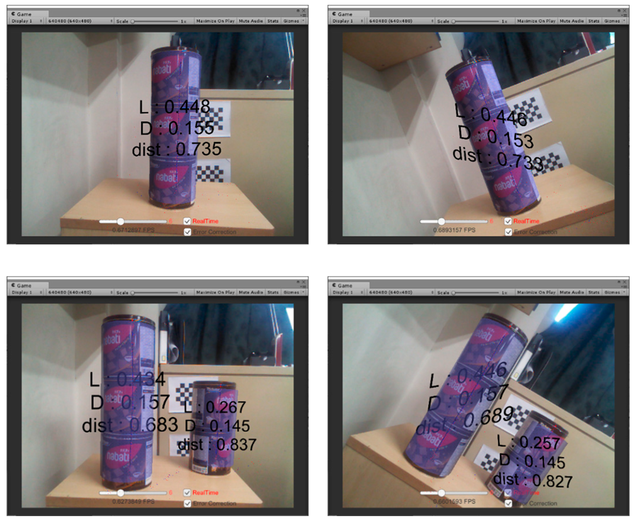
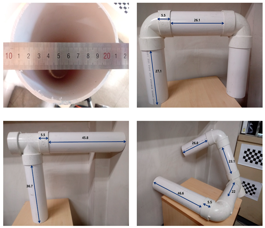
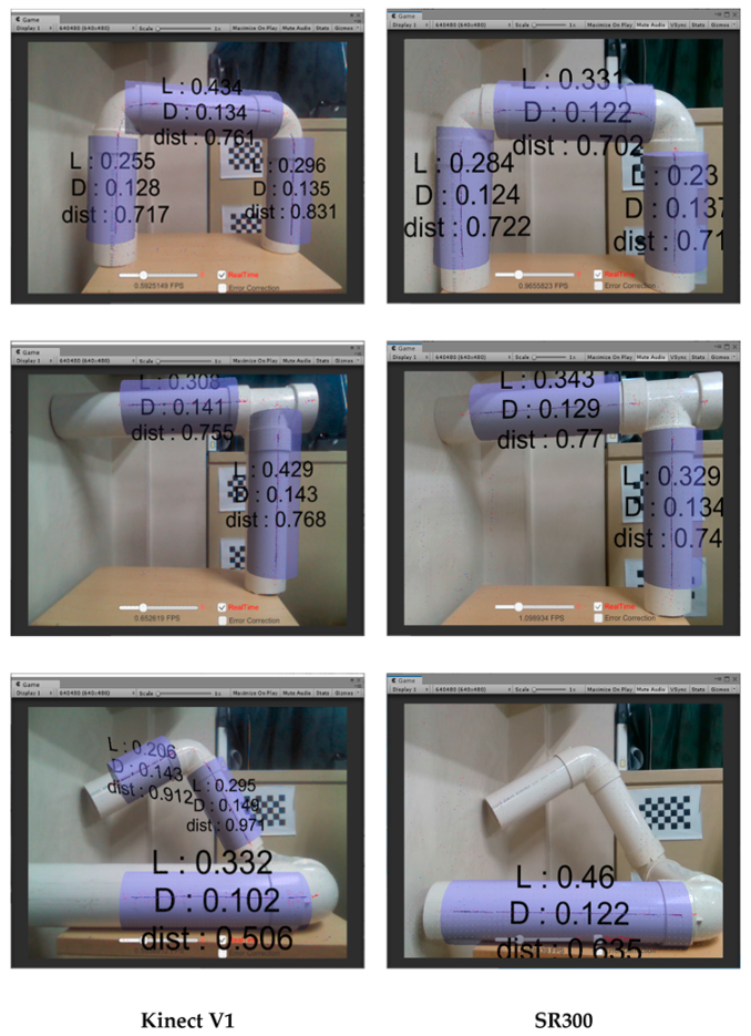
Figure 21 shows a 100 mm PVC pipe. As a result of the measurement, the inner diameter is 106 mm and the outer diameter is 114 mm. Using these PVC pipes, three types of composite pipelines were constructed, including 90°, T, and diagonal shapes

As demonstrated in Figure 22, the Kinect showed poor results compared to the SR300, unlike measurements with a 15 cm can. This is because the PVC pipes are small in diameter and cover a wider range. In the Kinect results, the left region of the T and composite pipes showed no point data.

This problem can be solved by setting the distance between the Kinect and PVC pipes far away; however, the accuracy lowers, making cylinder estimation impossible. SR300, on the other hand, generates data relatively accurately over a relatively large area, resulting in better pipe estimation than Kinect. However, if the distance is greater, the data may be inaccurate, resulting in a failure to measure a relatively long distance of pipe, such as the third pipe.

Figure 23 corrects the errors in the pipeline of Figure 22, as shown in Figure 13d. Both sensors showed results close to the PVC outside diameter. However, the overall accuracy of the point data was not enough to measure the bent area.

Based on the above results, we assumed that Kinect had a narrow width when measuring data and SR300 had a short measuring distance.

Kinect V1 and SR300 are inexpensive devices that can be easily used at home. Therefore, the products have clear advantages and disadvantages, and the accuracy varies greatly depending on the usage environment. However, correcting the matching results by considering the standard deviation will give an accurate estimate of the pipe with standardized values. However, if the matching result is corrected using the error ratio according to the distance, it is possible to accurately estimate the pipe with the standardized values.

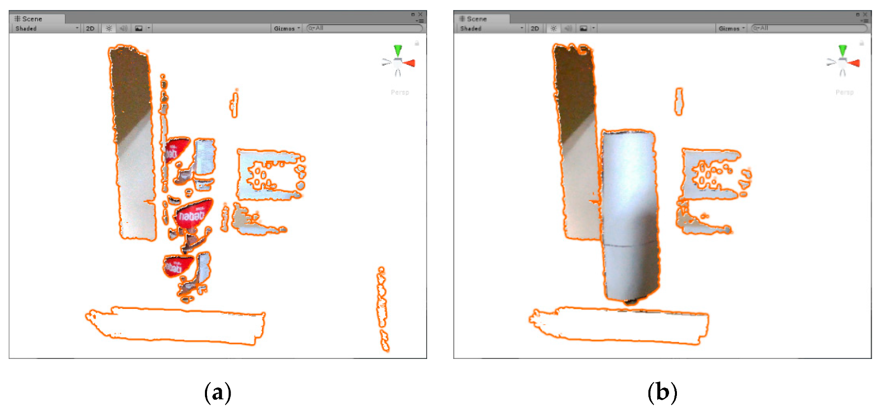
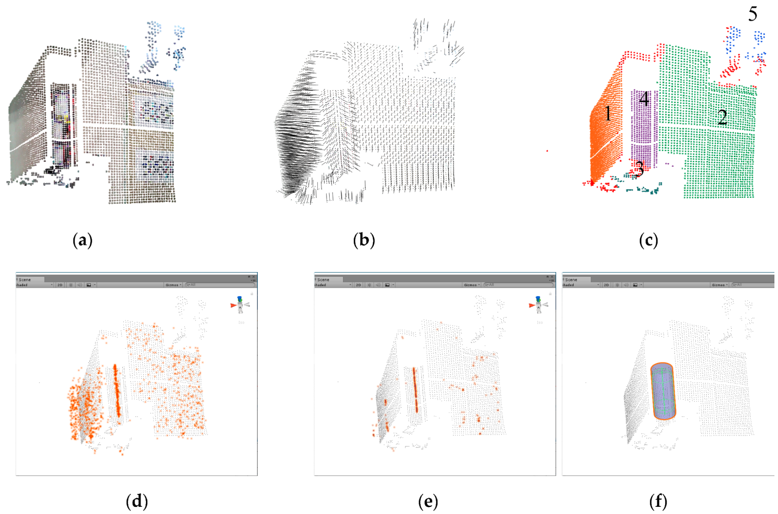
Based on the above results, they can be compared with the existing method as shown in Figure 24. The comparison used the data from Figure 10. The existing method was implemented using a point cloud library (pcl) [30].

Figure 24b shows that the normal estimation was well done. Figure 24c shows the results of segmentation based on the estimated normal. As a result, the segmentation was also performed well. However, in the process of confirming what type each group is based on the divided data, the cylinder shape was not predicted. In order to perform the Hough transform, the above process must be performed. Therefore, the existing method can no longer perform the cylinder estimation procedure. On the other hand, the fast cylinder matching method using RANSAC was able to estimate the central axis candidate as in (d) and filter as in (e), and as a result, predict the cylinder relatively accurately as in (f).

Looking at

Table 1. The result (Figure 24) of the existing method and fast cylinder matching method using RANSAC.

	Hough Transform Method	Fast Cylinder Matching Method
Execution time	201 ms (normal estimation + segmentation + cylinder candidate estimation)	181 ms (cylinder candidate data + filtering + cylinder estimation)
Results	number of inliers in each of 5 groups: 1, 1, 0, 1, 1 cylinder coefficient 1: 320.86, 146.06, 647.05, −0.27, 0.54, 0.79, 0.15 2: −226.42, 453.54, 1159.33, −0.72, −0.65, −0.20, 0.34 3: 4: 12.51, −151.34, 837.76, 0.31, 0.94, −0.06, 0.24 5: −693.46, 456.648, 1318.97, 0.31, 0.45, 0.83, 0.06	RANSAC error threshold: 0.02, 0.05 (cm) ϵ= 80, 340 pts., 179 ms (first step), 1cyl. 2 ms (second step) 1: diameter = 0.162 m, length = 0.207 m

, the existing method performed normal estimation and segmentation in 201 ms, and it determined whether each group was a cylinder. However, the number of points corresponding to the cylinder in each group were 1,1,0,1,1, and it was not possible to determine whether each group was a cylinder or not. In addition, according to Figure 24c, the cylinder group was group 4. The mathematical parameters of group 4 were 12.51, −151.34, 837.76, 0.31, 0.94, −0.06, and 0.24. These are the position (x, y, z), direction (x, y, z), and radius, respectively. Here, the final factor, 0.24, was the radius of this cylinder, which is not correct. On the other hand, the fast cylinder matching method using RANSAC estimated the cylinder at 181 ms, sampled at an 80% ratio to find the candidate cylinder for 340 p at 179 ms, and estimated one cylinder at 2 ms.

The estimated cylinder was 16.2 cm in diameter and 20.7 cm in length. Looking at the above results, both the execution time and the results were more accurate than the existing methods. The existing method could not estimate the cylinder candidate; thus, it could not perform cylinder estimation using the Hough transform. The Hough transform is generally known to consume a lot of execution time and resources. We estimated that the amount of point data was small as the existing method failed to estimate the cylinder candidate, or data obtained from one side of the actual cylinder may be unsuitable with the existing method. Therefore, the fast cylinder matching method using RANSAC and the proposed method were suitable for real-time estimation for augmented reality.

4. Conclusions

This paper aimed to obtain point data from depth images, to estimate cylinders as quickly as possible, and then to visualize them. When considering these goals, fast pipe matching has also been shown to be feasible in real-time cylinder estimation. Although using Kinect V1 has shown a lack of point data accuracy and data acquisition speed, the real-time estimation using multiple cores was close to 2.5 frames. The SR300 sensor based on coded light estimated the cylinder at a slightly faster speed. Of course, the matching result was rather poor as it was a pipe estimation using a point cloud constructed based on one side rather than exact data obtained through a laser scanner and registration. However, it was possible to increase the accuracy by correcting the error through empirically checking the mean error. In general, pipes are manufactured in standard sizes; therefore, the diameter of the installed pipes can be predicted relatively accurately.

Although there are errors, the matching results can be confirmed quickly through real-time processing. These methods can be used in various areas when applied to AR devices to be developed. If the proposed method is compiled and executed in the form of parallel processing using a graphics processing unit (GPU), cloud computing, and the optimization of the source code and distribution, this will perform better than our experimental results. The proposed method used RASNAC and PCA methods repeatedly. RASNAC is a methodology that determines the parameters by finding the optimal hypothesis through sampling. PCA is a methodology that analyzes the directivity of data through eigenvalue/eigenvector decomposition using singular value decomposition (SVD) after constructing a covariance matrix. As the above methods are simple calculations, parallel processing is possible. The authors in [31] proposed a fast and robust RANSAC framework through a GPU, and the researchers in [32] proposed a singular value decomposition (SVD) using cuda cores. The reason the above method can be calculated faster on a GPU is because the structure is simple and there are many partial calculations that can be processed simultaneously.

The fast cylinder matching method using RANSAC enabled fast cylinder-like pipe estimation by local segmentation sampling in the point cloud. The sphere fitting was shown to be suitable for estimating the central axis of the cylinder, and the data were randomly extracted for fast processing. The constructed central axis data could confirm the direction through principal component analysis. We improved the work efficiency of manual modeling by using linear and curved cylinder estimation followed by central axis estimation without constraints and segmentation. Real-time estimation can also be performed to confirm the cylinder information quickly through an AR camera in the field.

It is unfortunate that we could only perform tests on easily available devices (Kinect, SR300); however, we expect that our proposed method will work on most devices that can acquire depth images.

In the future, research will be conducted to smoothly integrate the estimated straight lines and curves into one, and to increase the performance through parallel processing or cloud computing with efficient memory partitioning, to derive fast, accurate, and consistent results.

References

1. Lee, M.; Lee, S.; Kwon, S.; Chin, S. A study on scan data matching for reverse engineering of pipes in plant construction. KSCE J. Civ. Eng. 2017, 21, 2027–2036. [Google Scholar] [CrossRef]
2. Rabbani, T.; Van Den Heuvel, F. Efficient hough transform for automatic detection of cylinders in point clouds. Isprs Wg Iii/3 Iii/4 2005, 3, 60–65. [Google Scholar]
3. Hackel, T.; Savinov, N.; Ladicky, L.; Wegner, J.D.; Schindler, K.; Pollefeys, M. Semantic3d. net: A new large-scale point cloud classification benchmark. arXiv arXiv:1704.03847.
4. Su, Y.-T.; Bethel, J. Detection and robust estimation of cylinder features in point clouds. In Proceedings of the ASPRS Annual Conference on Opportunities for Emerging Geospatial Technologies, San Diego, CA, USA, 26–30 April 2010. [Google Scholar]
5. Liu, Y.J.; Zhang, J.B.; Hou, J.C.; Ren, J.C.; Tang, W.Q. Cylinder detection in large-scale point cloud of pipeline plant. IEEE Trans. Visual. Comput. Graphics 2013, 19, 1700–1707. [Google Scholar] [CrossRef] [PubMed] [Green Version]
6. Huang, J.; You, S. Detecting objects in scene point cloud: A combinational approach. In Proceedings of the 2013 International Conference on 3D Vision-3DV 2013, Seattle, WA, USA, 29 June–1 July 2013. [Google Scholar]
7. Ahmed, M.F.; Haas, C.T.; Haas, R. Automatic detection of cylindrical objects in built facilities. J. Comput. Civ. Eng. 2014, 28, 04014009. [Google Scholar] [CrossRef]
8. Patil, A.K.; Holi, P.; Lee, S.K.; Chai, Y.H. An adaptive approach for the reconstruction and modeling of as-built 3D pipelines from point clouds. Autom. Constr. 2017, 75, 65–78. [Google Scholar] [CrossRef]
9. Kim, J.Y. Investigative Analysis of Virtual Reality Technology through Case Study. J. Next-Gener. Converg. Inf. Serv. Technol. 2014, 3, 101–108. [Google Scholar]
10. Kang, H.S.; Kim, J.Y. Analysis of Interaction Items in the Virtual Reality Game Interface. KSCG 2018, 31, 185–195. [Google Scholar]
11. Youm, D.; Seo, S.; Kim, J.Y. Design and development methodologies of Kkongalmon, a location-based augmented reality game using mobile geographic information. EURASIP J. Image Video Process. 2019, 1, 1. [Google Scholar] [CrossRef] [Green Version]
12. Wikipedia. Available online: https://en.wikipedia.org/wiki/Augmented_reality (accessed on 24 February 2020).
13. Gupta, S.; Lohani, B. Augmented reality system using lidar point cloud data for displaying dimensional information of objects on mobile phones. ISPRS Ann. Photogramm. Remote Sens. Spat. Inf. Sci. 2014, 2, 153. [Google Scholar] [CrossRef] [Green Version]
14. Placitelli, A.P.; Gallo, L. Low-cost augmented reality systems via 3D point cloud sensors. In Proceedings of the 2011 Seventh International Conference on Signal Image Technology & Internet-Based Systems, Dijon, France, 28 November–1 December 2011; pp. 188–192. [Google Scholar]
15. Gao, Q.H.; Wan, T.R.; Tang, W.; Chen, L. Object registration in semi-cluttered and partial-occluded scenes for augmented reality. Multimed. Tools Appl. 2019, 78, 15079–15099. [Google Scholar] [CrossRef] [Green Version]
16. Mancera-Taboada, J.; Rodríguez-Gonzálvez, P.; González-Aguilera, D.; Finat, J.; San José, J.; Fernández, J.J.; Martínez, R. From the point cloud to virtual and augmented reality: Digital accessibility for disabled people in San Martin’s Church (Segovia) and its surroundings. In International Conference on Computational Science and Its Applications; Springer: Berlin/Heidelberg, Germany, 2011; pp. 303–317. [Google Scholar]
17. Schwarz, S.; Pesonen, M. Real-time decoding and AR playback of the emerging MPEG video-based point cloud compression standard. In Nokia Technologies; IBC: Helsinki, Finland, 2019. [Google Scholar]
18. Mahmood, B.; Han, S. 3D Registration of Indoor Point Clouds for Augmented Reality. In Proceedings of the ASCE International Conference on Computing in Civil, Atlanta, GA, USA, 17–19 June 2019. [Google Scholar]
19. Kung, Y.C.; Huang, Y.L.; Chien, S.Y. Efficient Surface Detection for Augmented Reality on 3D Point Clouds. In Proceedings of the 33rd Computer Graphics International, Association for Computing Machinery, New York, NY, USA, June 2016; pp. 89–92. [Google Scholar]
20. Pavez, E.; Chou, P.A.; De Queiroz, R.L.; Ortega, A. Dynamic polygon clouds: Representation and compression for VR/AR. APSIPA Trans. Signal Inf. Process. 2018, 7, e15. [Google Scholar] [CrossRef] [Green Version]
21. Cazamias, J.; Raj, A. Virtualized Reality Using Depth Camera Point Clouds; Stanford EE 267: Stanford, CA, USA, 2016. [Google Scholar]
22. Jimeno-Morenilla, A.; Sánchez-Romero, J.L.; Salas-Pérez, F. Augmented and virtual reality techniques for footwear. Comput. Ind. 2013, 64, 1371–1382. [Google Scholar] [CrossRef] [Green Version]
23. Fischler, M.A.; Bolles, R.C. Random sample consensus: A paradigm for model fitting with applications to image analysis and automated cartography. Commun. ACM 1981, 24, 381–395. [Google Scholar] [CrossRef]
24. Wikipedia. Available online: https://en.wikipedia.org/wiki/Random_sample_consensus (accessed on 24 February 2020).
25. Smith, L.I. A Tutorial on Principal Components Analysis; Cornell University: Ithaca, NY, USA, 2002. [Google Scholar]
26. Wikipedia. Available online: https://en.wikipedia.org/wiki/Principal_component_analysis (accessed on 24 February 2020).
27. Jin, Y.-H.; Lee, W.-H. Fast Cylinder Shape Matching Using Random Sample Consensus in Large Scale Point Cloud. Appl. Sci. 2019, 9, 974. [Google Scholar] [CrossRef] [Green Version]
28. Carfagni, M.; Furferi, R.; Governi, L.; Servi, M.; Uccheddu, F.; Volpe, Y. On the performance of the Intel SR300 depth camera: Metrological and critical characterization. IEEE Sens. J. 2017, 17, 4508–4519. [Google Scholar] [CrossRef] [Green Version]
29. Zabatani, A.; Surazhsky, V.; Sperling, E.; Moshe, S.B.; Menashe, O.; Silver, D.H.; Kimmel, R. Intel® RealSense™ SR300 Coded light depth Camera. IEEE Trans. Pattern Anal. Mach. Intell. 2019. [Google Scholar] [CrossRef] [PubMed]
30. Pcl. Available online: http://www.pointclouds.org (accessed on 24 February 2020).
31. Roters, J.; Jiang, X. FestGPU: A framework for fast robust estimation on GPU. J. Real Time Image Process. 2017, 13, 759–772. [Google Scholar] [CrossRef]
32. Lahabar, S.; Narayanan, P.J. Singular value decomposition on GPU using CUDA. In Proceedings of the 2009 IEEE International Symposium on Parallel & Distributed Processing, Rome, Italy, 23–29 May 2009; pp. 1530–2075. [Google Scholar]
Figure 1. Model recognition pre-processing process.
Electronics 09 00836 g001
Figure 2. The Hough transform process: (a) 3D transform for the direction; (b) 2D transform for the diameter.
Electronics 09 00836 g002
Figure 3. The proposed real-time augmented reality visualization method.
Electronics 09 00836 g003
Figure 4. Center estimation using the trace of a sphere.
Electronics 09 00836 g004
Figure 5. Principal component analysis (PCA) eigenvector.
Electronics 09 00836 g005
Figure 6. Searching method for center axis estimation: (a) eigenvector at a point; (b) sum of the eigenvectors; (c) matching cylinder result through vector summation.
Electronics 09 00836 g006
Figure 7. Control point estimation using PCA: (a) estimation of the tangent line at one point; (b) estimation of the spline control point using intersections of the tangent lines; (c) the curve matching result.
Electronics 09 00836 g007
Figure 8. Single vs. multi core memory usage: (a) single core with one KDTree; (b) multi core with four KDTrees (The red box is a part used in the entire domain).
Electronics 09 00836 g008
Figure 9. Cylinder estimation with four-core multithreading: (a) the point cloud partition for use with four cores and KDTree; (b) the central axis estimation and integration for each result.
Electronics 09 00836 g009
Figure 10. Point down sampling using a voxel grid: (a) Kinect rgb image and point cloud 248,935 p from depth image; (b) point cloud down sampling 55,328 p.
Electronics 09 00836 g010
Figure 11. Center axis estimation through multiple frames: (a) results of the sphere fitting of each frame; (b) results of the central axis estimation with noise filtering through integrating the results of (a) with one or more frames.
Electronics 09 00836 g011
Figure 12. Point data scale k times for estimation ϵ = 25: (a) the default scale; (b) the k times scale.
Electronics 09 00836 g012
Figure 13. Single frame center axis estimation: (a) default unit; (b) virtual cylinder using three default units; (c) cylinder matching result; (d) error correction using the diameter. (c, d is in meters).
Electronics 09 00836 g013aElectronics 09 00836 g013b
Figure 14. Errors due to distance (m).
Electronics 09 00836 g014aElectronics 09 00836 g014b
Figure 15. Multi frames center axis estimation (cm).
Electronics 09 00836 g015
Figure 16. Real-time cylinder estimation using multiple (6) cores (cm).
Electronics 09 00836 g016
Figure 17. Phase-shift sensor real-time matching results for six cores and six frames; FOV = 48.6°; ϵ = 50 error correction mode (m).
Electronics 09 00836 g017
Figure 18. Intel RealSense SR300 sensor.
Electronics 09 00836 g018
Figure 19. Characteristics of the SR300 sensor: (a) A diffuse reflection due to the characteristics of the can material; (b) surface treatment to reduce diffuse reflections.
Electronics 09 00836 g019
Figure 20. Time of flight sensor real-time matching results for six cores and six frames. FOV = 41.5°; ϵ = 50 error correction mode (m).
Electronics 09 00836 g020
Figure 21. Three types of pipeline with 100 mm polyvinyl chloride (PVC) (cm).
Electronics 09 00836 g021
Figure 22. Real-time matching results with six cores and six frames; ϵ = 50. (m)
Electronics 09 00836 g022
Figure 23. Real-time matching results for six cores and six frames; ϵ = 50 error correction mode. (m)
Electronics 09 00836 g023
Figure 24. Pre-processing for the Hough transform and fast cylinder matching method using random sample consensus (RANSAC): (a) uniformized data; (b) normal estimation; (c) segmentation; (d) center line estimation; (e) filtered center line estimation; and (f) cylinder estimation.
Electronics 09 00836 g024