An Advanced Pruning Method in the Architecture of Extreme Learning Machines Using L1-Regularization and Bootstrapping

 ,
,  , , and
Abstract
1. Introduction
2. Related Work
2.1. Extreme Learning Machines
2.2. Pruning and Regularized Methods for Extreme Learning Machines
2.3. Extreme Learning Machine and Pattern Recognition Problems
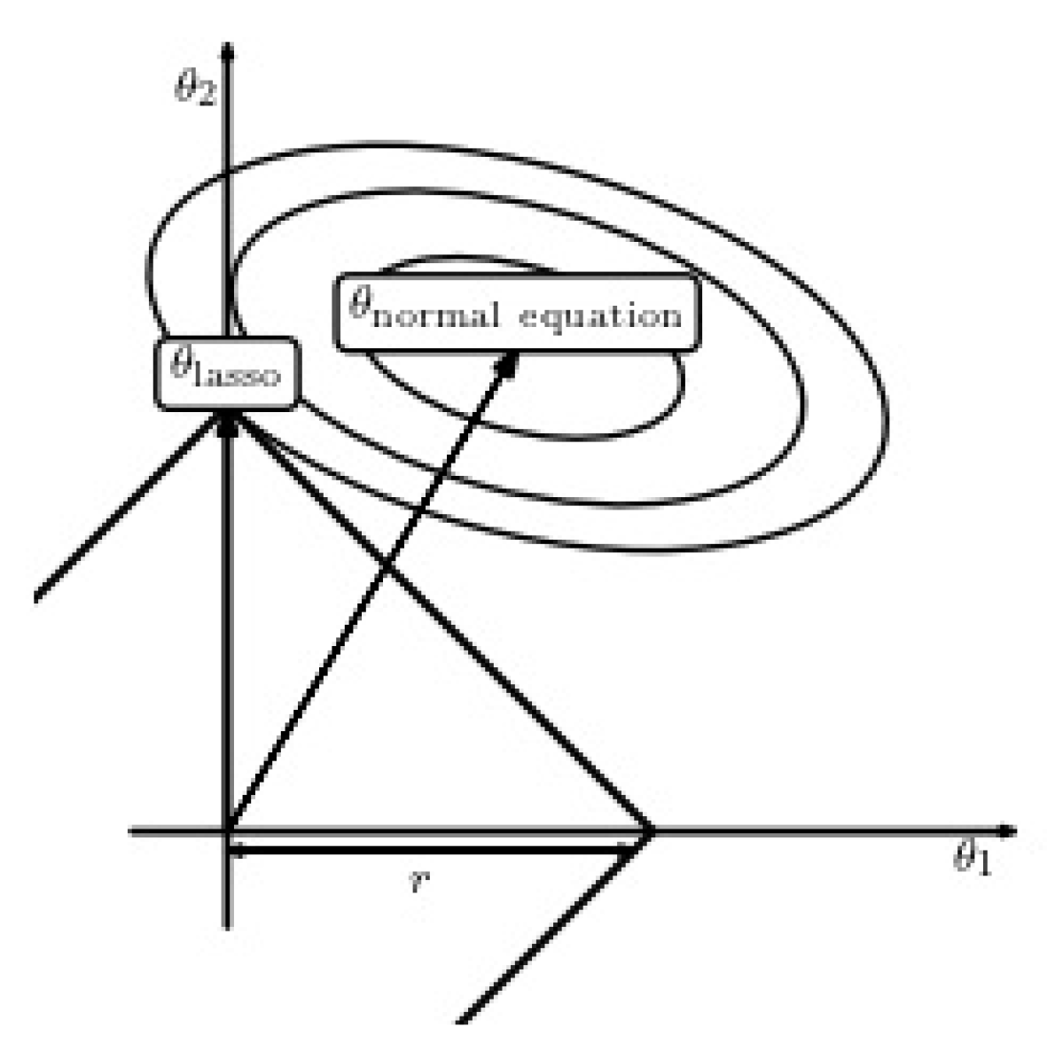
2.4. Determining Coefficients of Linear Regression in a Robust Manner with L1-Regularization
3. Pruning ELM Using Bootstrapped Lasso (BR-ELM)
| Algorithm 1 Bolasso-bootstrap-enhanced least absolute shrinkage operator |
| (1) Let n be the number of examples, (lines) in X and Y: (2) Draw n examples from , uniformly and with replacement, termed as (, ). (3) Perform LARS on (, ) with a given value of to estimate the regression coefficients . (4) Determine which coefficients are nonzero. (5) Repeat steps (2) to (4) for a specified number of bootstraps . (6) Take the intersection of the non-zero coefficients from all bootstrap replications as significant variables to be selected (100% consensus). (7) Revise using the variables selected via non-regularized least squares regression (if requested). (8) Calculate the expected error of the model on a separate validation set. (9) Repeat the procedure for each value of bootstraps and (actually done more efficiently by collecting interim results). (10) Determine “optimal” values for and b through eliciting the minimal expected error of the model on a separate validation set. |
- The number of bootstrap replicates, ;
- The consensus threshold, .
- The initial amount of hidden neurons, k
| Algorithm 2 Pruning algorithm for Extreme Learning Machines |
| (1) Define number of bootstrap replicates. (2) Define the consensus threshold . (3) Create initial hidden neurons k following the conventional strategy used in ELMs. (4) Assign random values to and , for j = 1, …, k. (5) For : (6) Draw n examples from , uniformly and with replacement, termed as (, ). (7) Compute using Equation (2). (8) Perform LARS algorithm in order to solve (4) for yielding (internally, apply regularization parameter choice technique to elicit the optimal ). (9) EndFor (10) Select the final neurons using (7) through (6) with consensus threshold . (11) Construct matrix from the selected neurons. (11) Estimate the final output layer weights by applying (3) using instead of G. (12) Define the output hidden layer using (8). |
4. Experiments
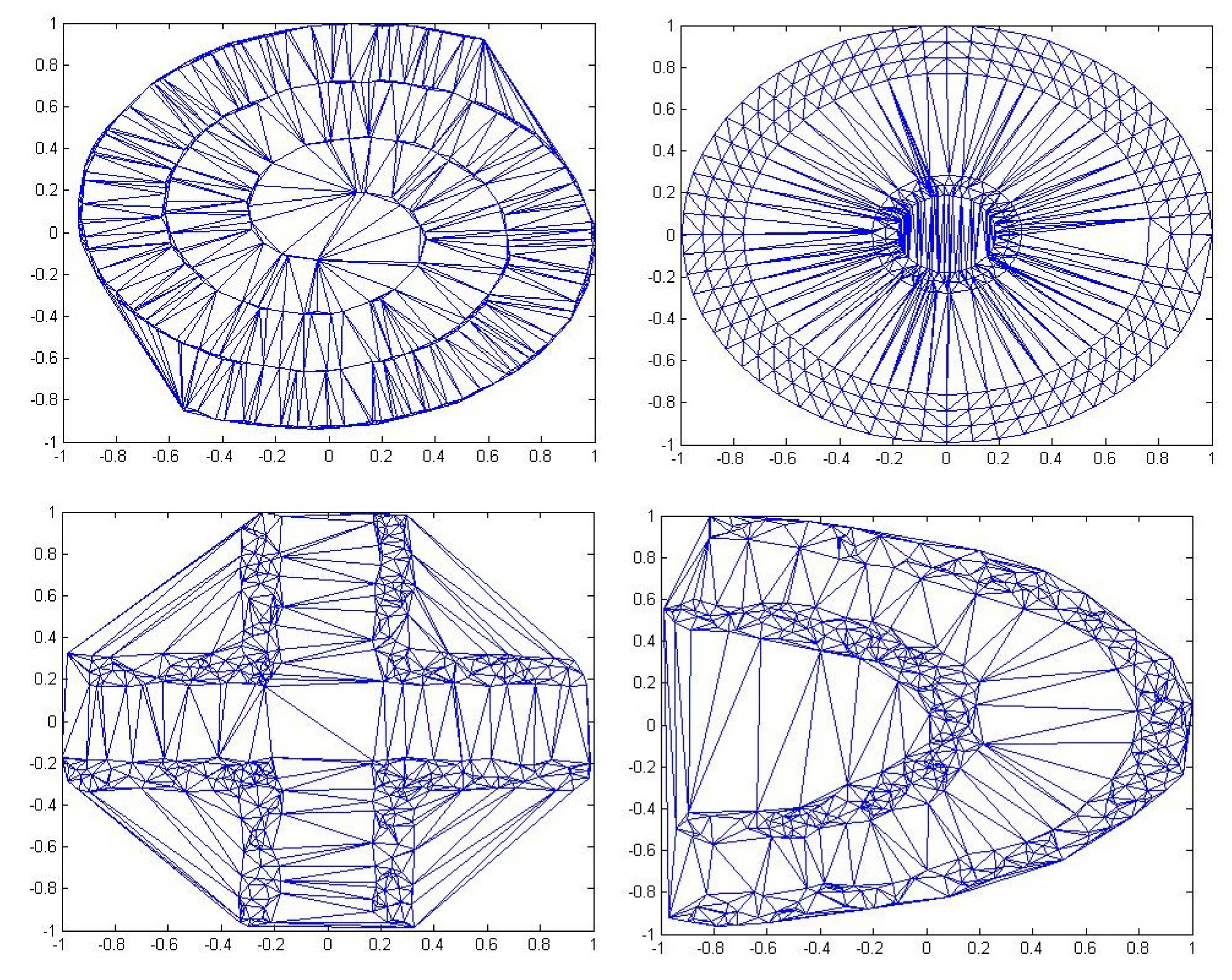
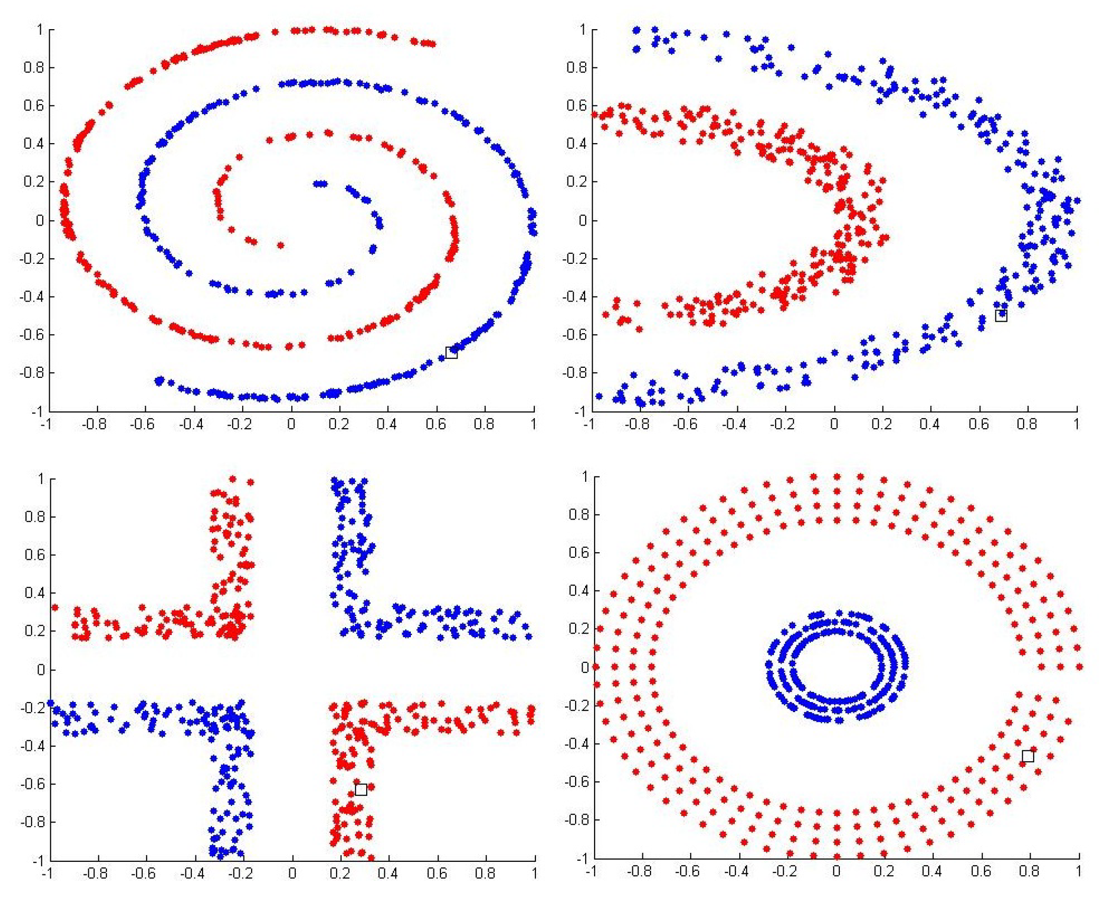
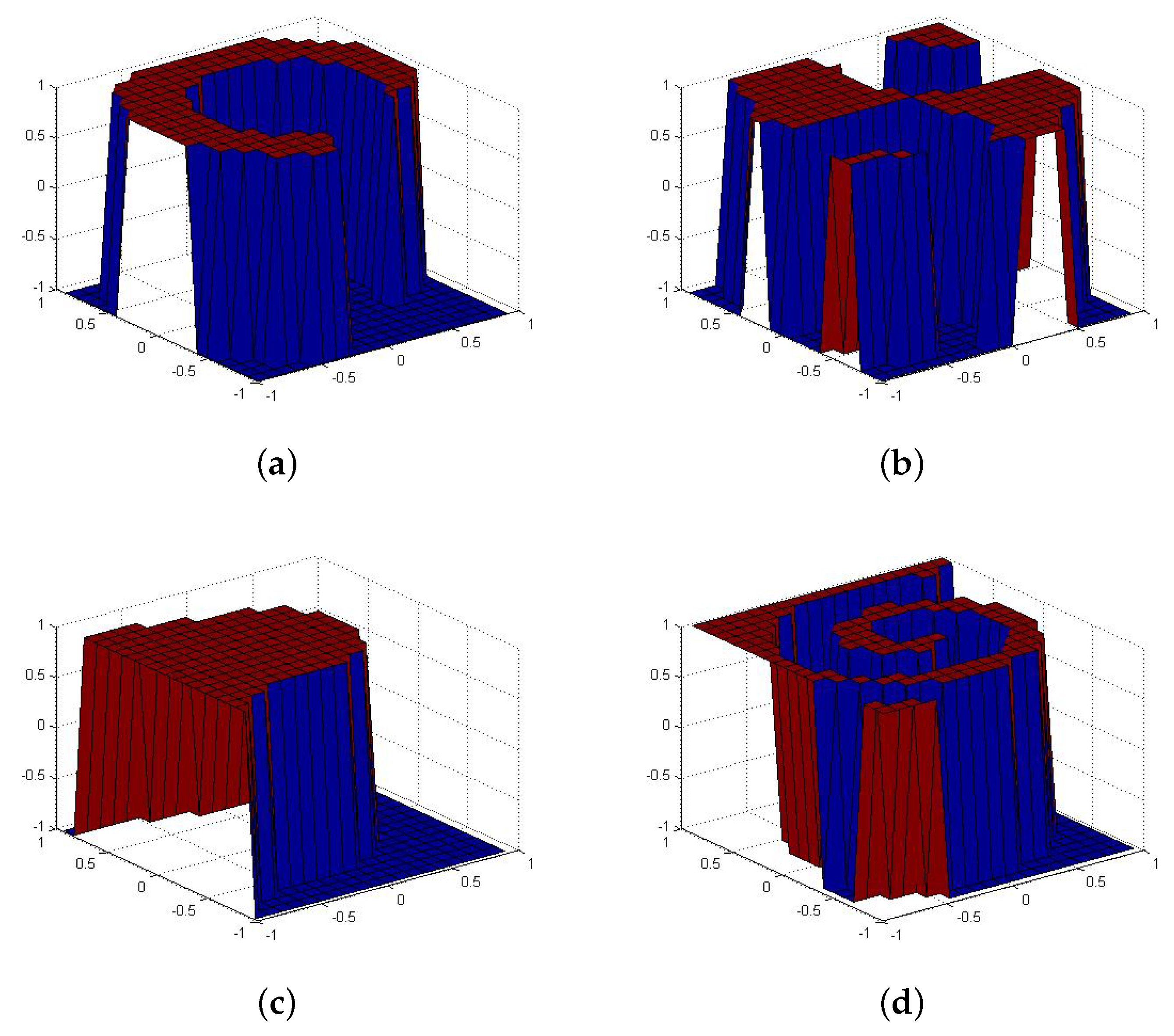
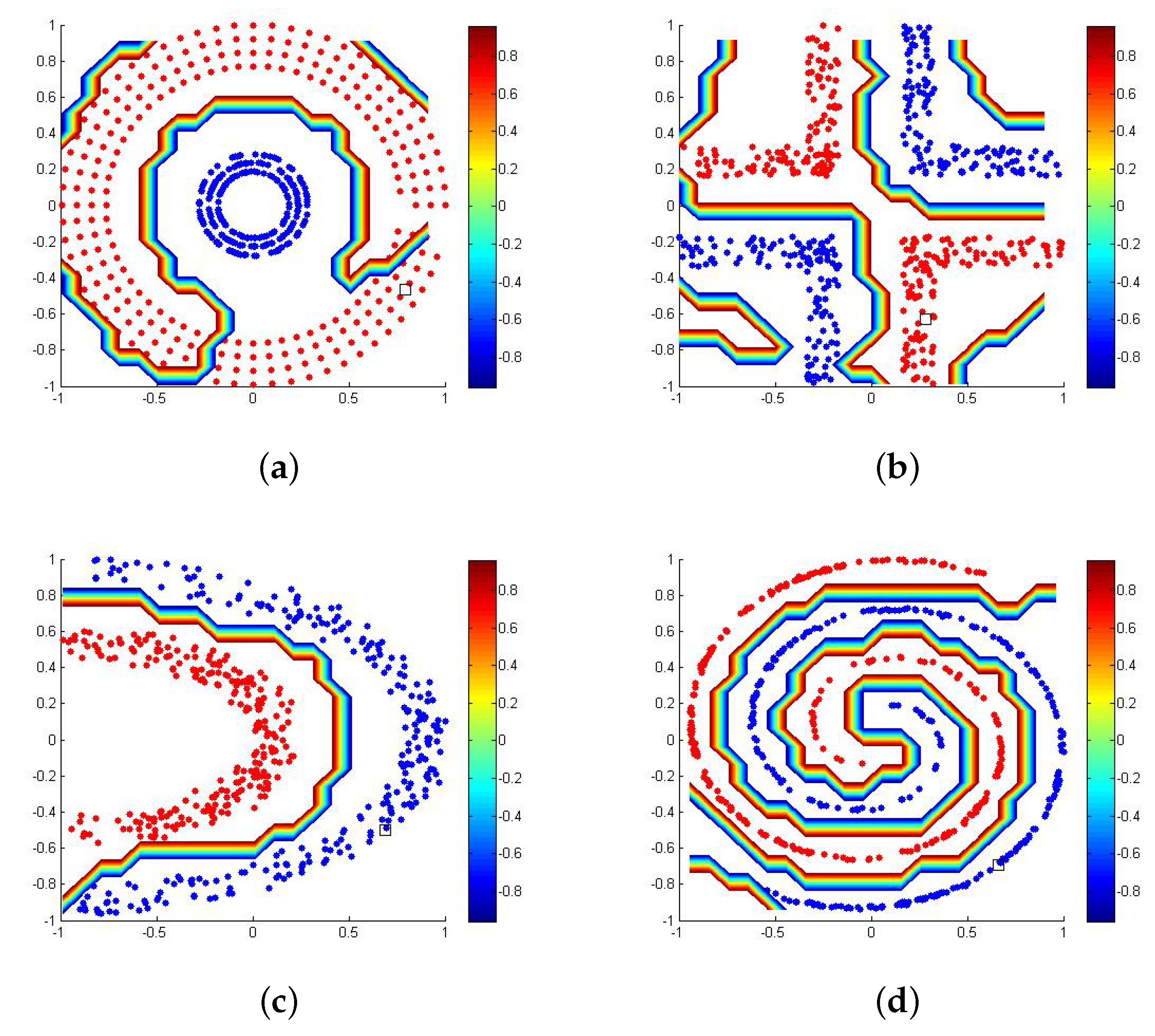
4.1. Synthetic Database Classification
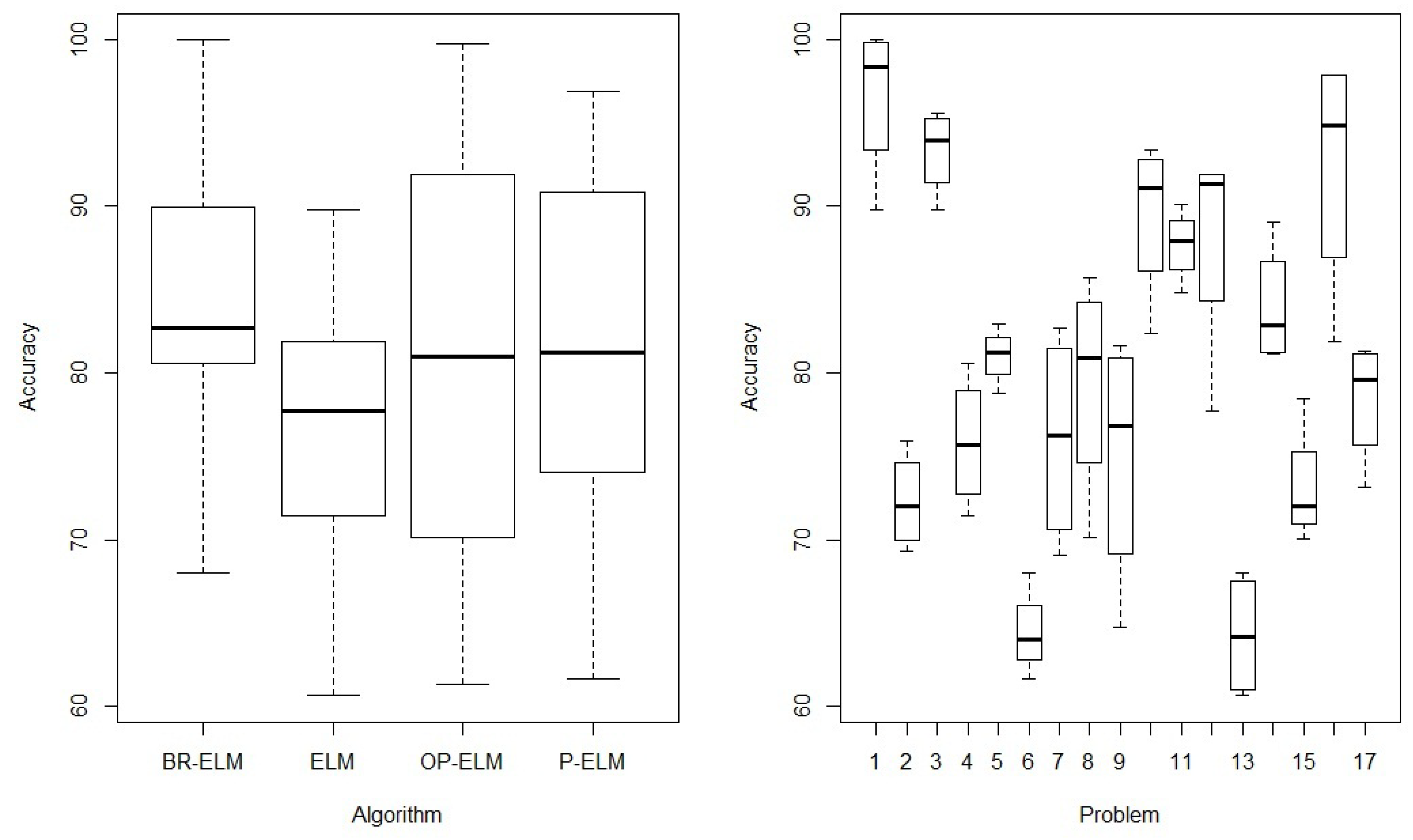
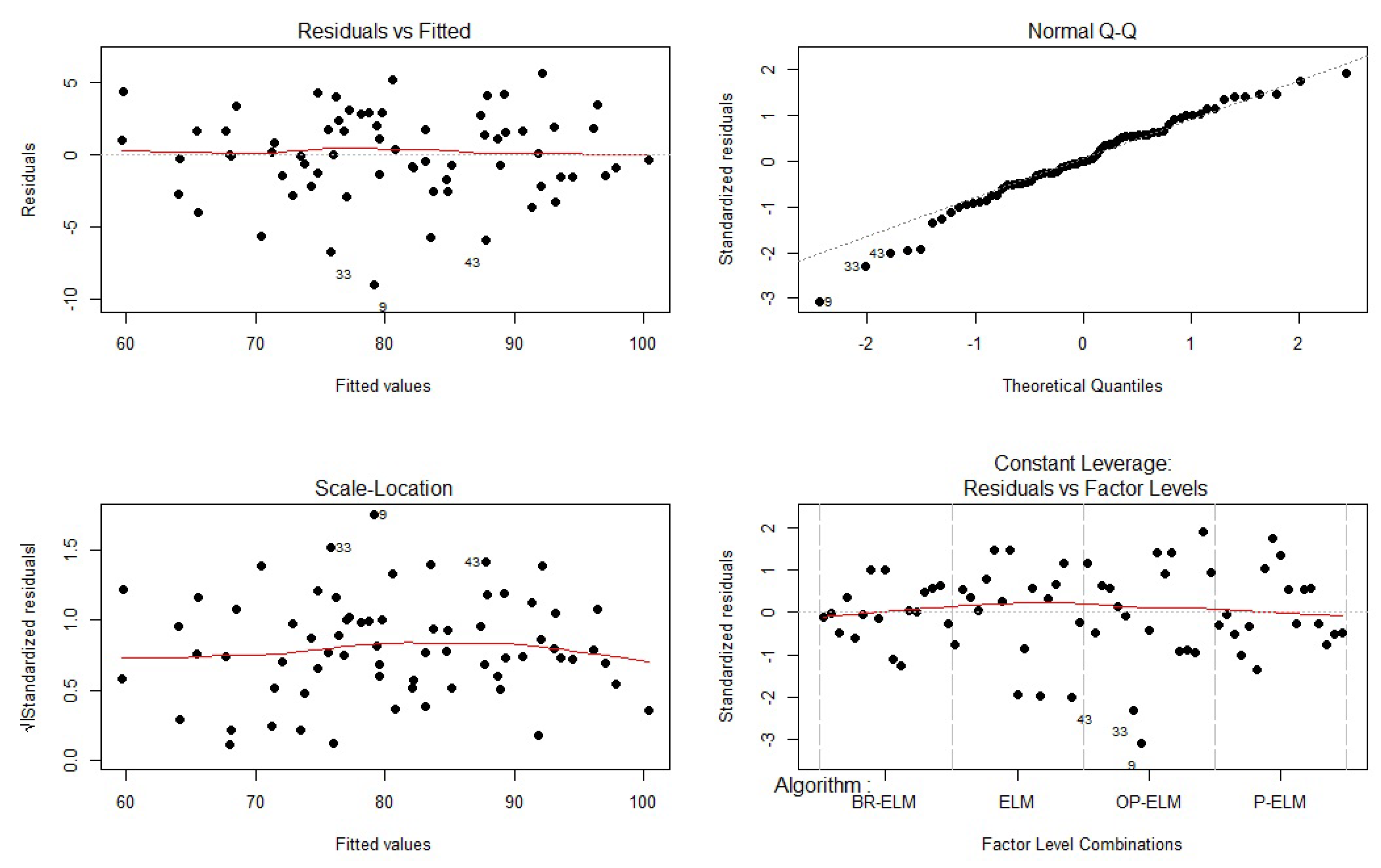
4.2. Evaluation Measures Used for Tests on Real-World Data Sets
4.3. Benchmark Classification Datasets
4.4. Benchmark Regression Datasets
- Datasets with low size and low dimensions, for example, Carbon nanotubes [57].
4.5. Pattern Classification Tests Using Complex Real Datasets
4.5.1. Objectivity or Subjectivity of Sporting Articles
4.5.2. Suspicious Firm Classification
5. Conclusions
Author Contributions
Funding
Acknowledgments
Conflicts of Interest
References
- Broomhead, D.S.; Lowe, D. Radial Basis Functions, Multi-Variable Functional Interpolation and Adaptive Networks; Technical Report; Royal Signals and Radar Establishment Malvern: Malvern, UK, 1988. [Google Scholar]
- Pao, Y.H.; Park, G.H.; Sobajic, D.J. Learning and generalization characteristics of the random vector functional-link net. Neurocomputing 1994, 6, 163–180. [Google Scholar] [CrossRef]
- Huang, G.B.; Zhu, Q.Y.; Siew, C.K. Extreme learning machine: Theory and applications. Neurocomputing 2006, 70, 489–501. [Google Scholar] [CrossRef]
- Miche, Y.; Sorjamaa, A.; Bas, P.; Simula, O.; Jutten, C.; Lendasse, A. OP-ELM: Optimally pruned extreme learning machine. IEEE Trans. Neural Netw. 2010, 21, 158–162. [Google Scholar] [CrossRef] [PubMed]
- Rong, H.J.; Ong, Y.S.; Tan, A.H.; Zhu, Z. A fast pruned-extreme learning machine for classification problem. Neurocomputing 2008, 72, 359–366. [Google Scholar] [CrossRef]
- Similä, T.; Tikka, J. Multiresponse Sparse Regression with Application to Multidimensional Scaling. In Artificial Neural Networks: Formal Models and Their Applications—ICANN 2005; Duch, W., Kacprzyk, J., Oja, E., Zadrożny, S., Eds.; Springer: Berlin/Heidelberg, Germany, 2005; pp. 97–102. [Google Scholar]
- Efron, B.; Hastie, T.; Johnstone, I.; Tibshirani, R. Least angle regression. Ann. Stat. 2004, 32, 407–499. [Google Scholar] [CrossRef]
- Bach, F.R. Bolasso: Model Consistent Lasso Estimation Through the Bootstrap. In Proceedings of the 25th International Conference on Machine Learning; ACM: New York, NY, USA, 2008; pp. 33–40. [Google Scholar] [CrossRef]
- Breiman, L. Bagging Predictors. Mach. Learn. 1996, 24, 123–140. [Google Scholar] [CrossRef]
- Pao, Y.H.; Takefuji, Y. Functional-link net computing: Theory, system architecture, and functionalities. Computer 1992, 25, 76–79. [Google Scholar] [CrossRef]
- Martínez-Martínez, J.M.; Escandell-Montero, P.; Soria-Olivas, E.; Martín-Guerrero, J.D.; Magdalena-Benedito, R.; Gómez-Sanchis, J. Regularized extreme learning machine for regression problems. Neurocomputing 2011, 74, 3716–3721. [Google Scholar] [CrossRef]
- Ljung, L. System Identification: Theory for the User; Prentice Hall PTR, Prentic Hall Inc.: Upper Saddle River, NJ, USA, 1999. [Google Scholar]
- James, G.; Witten, D.; Hastie, T.; Tibshirani, R. An Introduction to Statistical Learning; Springer: Berlin/Heidelberg, Germany, 2013; Volume 112. [Google Scholar]
- Tikhonov, A.N. On the solution of ill-posed problems and the method of regularization. In Doklady Akademii Nauk; Russian Academy of Sciences: Moscow, Russia, 1963; Volume 151, pp. 501–504. [Google Scholar]
- Bauer, F.; Lukas, M. Comparing parameter choice methods for regularization of ill-posed problems. Math. Comput. Simul. 2011, 81, 1795–1841. [Google Scholar] [CrossRef]
- Csáji, B.C. Approximation with artificial neural networks. Fac. Sci. Etvs Lornd Univ. Hung. 2001, 24, 48. [Google Scholar]
- Miche, Y.; van Heeswijk, M.; Bas, P.; Simula, O.; Lendasse, A. TROP-ELM: A double-regularized ELM using LARS and Tikhonov regularization. Neurocomputing 2011, 74, 2413–2421. [Google Scholar] [CrossRef]
- Yu, Q.; Miche, Y.; Eirola, E.; van Heeswijk, M.; Séverin, E.; Lendasse, A. Regularized extreme learning machine for regression with missing data. Neurocomputing 2013, 102, 45–51. [Google Scholar] [CrossRef]
- Hastie, T.; Tibshirani, R.; Friedman, J.; Franklin, J. The Elements of Statistical Learning: Data Mining, Inference and Prediction; Springer: Berlin/Heidelberg, Germany, 2005; Volume 27, pp. 83–85. [Google Scholar]
- Escandell-Montero, P.; Martínez-Martínez, J.M.; Soria-Olivas, E.; Guimerá-Tomás, J.; Martínez-Sober, M.; Serrano-López, A.J. Regularized Committee of Extreme Learning Machine for Regression Problems. In Proceedings of the European Symposium on Artificial Neural Networks, Computational Intelligence and Machine Learning, ESANN 2012, Bruges, Belgium, 25–27 April 2012; pp. 251–256. [Google Scholar]
- Kuncheva, L. Combining Pattern Classifiers: Methods and Algorithms; Wiley-Interscience (John Wiley & Sons): Chichester, West Sussex, UK, 2004. [Google Scholar]
- Kassani, P.H.; Teoh, A.B.J.; Kim, E. Sparse pseudoinverse incremental extreme learning machine. Neurocomputing 2018, 287, 128–142. [Google Scholar] [CrossRef]
- Zhao, Y.P.; Pan, Y.T.; Song, F.Q.; Sun, L.; Chen, T.H. Feature selection of generalized extreme learning machine for regression problems. Neurocomputing 2018, 275, 2810–2823. [Google Scholar] [CrossRef]
- Xu, S.; Wang, J. Dynamic extreme learning machine for data stream classification. Neurocomputing 2017, 238, 433–449. [Google Scholar] [CrossRef]
- Peng, Y.; Wang, S.; Long, X.; Lu, B.L. Discriminative graph regularized extreme learning machine and its application to face recognition. Neurocomputing 2015, 149, 340–353. [Google Scholar] [CrossRef]
- Huang, G.; Song, S.; Gupta, J.N.D.; Wu, C. Semi-Supervised and Unsupervised Extreme Learning Machines. IEEE Trans. Cybern. 2014, 44, 2405–2417. [Google Scholar] [CrossRef]
- Belkin, M.; Niyogi, P.; Sindhwani, V. Manifold regularization: A geometric framework for learning from labeled and unlabeled examples. J. Mach. Learn. Res. 2006, 7, 2399–2434. [Google Scholar]
- Silvestre, L.J.; Lemos, A.P.; Braga, J.P.; Braga, A.P. Dataset structure as prior information for parameter-free regularization of extreme learning machines. Neurocomputing 2015, 169, 288–294. [Google Scholar] [CrossRef]
- Pinto, D.; Lemos, A.P.; Braga, A.P.; Horizonte, B.; Gerais-Brazil, M. An affinity matrix approach for structure selection of extreme learning machines. In Proceedings; Presses universitaires de Louvain: Louvain-la-Neuve, Belgium, 2015; p. 343. [Google Scholar]
- Mohammed, A.A.; Minhas, R.; Wu, Q.J.; Sid-Ahmed, M.A. Human face recognition based on multidimensional PCA and extreme learning machine. Pattern Recognit. 2011, 44, 2588–2597. [Google Scholar] [CrossRef]
- Cao, J.; Zhang, K.; Luo, M.; Yin, C.; Lai, X. Extreme learning machine and adaptive sparse representation for image classification. Neural Netw. 2016, 81, 91–102. [Google Scholar] [CrossRef] [PubMed]
- Iosifidis, A.; Tefas, A.; Pitas, I. On the kernel extreme learning machine classifier. Pattern Recognit. Lett. 2015, 54, 11–17. [Google Scholar] [CrossRef]
- Xin, J.; Wang, Z.; Qu, L.; Wang, G. Elastic extreme learning machine for big data classification. Neurocomputing 2015, 149, 464–471. [Google Scholar] [CrossRef]
- Musikawan, P.; Sunat, K.; Kongsorot, Y.; Horata, P.; Chiewchanwattana, S. Parallelized Metaheuristic-Ensemble of Heterogeneous Feedforward Neural Networks for Regression Problems. IEEE Access 2019, 7, 26909–26932. [Google Scholar] [CrossRef]
- Liangjun, C.; Honeine, P.; Hua, Q.; Jihong, Z.; Xia, S. Correntropy-based robust multilayer extreme learning machines. Pattern Recognit. 2018, 84, 357–370. [Google Scholar] [CrossRef]
- Chen, B.; Wang, X.; Lu, N.; Wang, S.; Cao, J.; Qin, J. Mixture correntropy for robust learning. Pattern Recognit. 2018, 79, 318–327. [Google Scholar] [CrossRef]
- Gao, J.; Chai, S.; Zhang, B.; Xia, Y. Research on Network Intrusion Detection Based on Incremental Extreme Learning Machine and Adaptive Principal Component Analysis. Energies 2019, 12, 1223. [Google Scholar] [CrossRef]
- de Campos Souza, P.V.; Araujo, V.J.S.; Araujo, V.S.; Batista, L.O.; Guimaraes, A.J. Pruning Extreme Wavelets Learning Machine by Automatic Relevance Determination. In Engineering Applications of Neural Networks; Macintyre, J., Iliadis, L., Maglogiannis, I., Jayne, C., Eds.; Springer International Publishing: Cham, Switzerland, 2019; pp. 208–220. [Google Scholar]
- de Campos Souza, P.V. Pruning method in the architecture of extreme learning machines based on partial least squares regression. IEEE Lat. Am. Trans. 2018, 16, 2864–2871. [Google Scholar] [CrossRef]
- He, B.; Sun, T.; Yan, T.; Shen, Y.; Nian, R. A pruning ensemble model of extreme learning machine with L_{1/2} regularizer. Multidimens. Syst. Signal Process. 2017, 28, 1051–1069. [Google Scholar] [CrossRef]
- Fan, Y.T.; Wu, W.; Yang, W.Y.; Fan, Q.W.; Wang, J. A pruning algorithm with L 1/2 regularizer for extreme learning machine. J. Zhejiang Univ. Sci. C 2014, 15, 119–125. [Google Scholar] [CrossRef]
- Chang, J.; Sha, J. Prune Deep Neural Networks With the Modified L_{1/2} Penalty. IEEE Access 2018, 7, 2273–2280. [Google Scholar] [CrossRef]
- Alemu, H.Z.; Zhao, J.; Li, F.; Wu, W. Group L_{1/2} regularization for pruning hidden layer nodes of feedforward neural networks. IEEE Access 2019, 7, 9540–9557. [Google Scholar] [CrossRef]
- Xie, X.; Zhang, H.; Wang, J.; Chang, Q.; Wang, J.; Pal, N.R. Learning Optimized Structure of Neural Networks by Hidden Node Pruning With L1 Regularization. IEEE Trans. Cybern. 2019. [Google Scholar] [CrossRef]
- Schaffer, C. Overfitting Avoidance as Bias. Mach. Learn. 1993, 10, 153–178. [Google Scholar] [CrossRef]
- Islam, M.; Yao, X.; Nirjon, S.; Islam, M.; Murase, K. Bagging and Boosting Negatively Correlated Neural Networks. IEEE Trans. Syst. Man Cybern. Part B Cybern. 2008, 38, 771–784. [Google Scholar] [CrossRef] [PubMed]
- Murphy, K.P. Machine Learning: A Probabilistic Perspective; The MIT Press: Cambridge, MA, USA, 2012. [Google Scholar]
- Girosi, F.; Jones, M.; Poggio, T. Regularization Theory and Neural Networks Architectures. Neural Comput. 1995, 7, 219–269. [Google Scholar] [CrossRef]
- Tibshirani, R. Regression shrinkage and selection via the lasso. J. R. Stat. Soc. 1996, 58B, 267–288. [Google Scholar] [CrossRef]
- Efron, B.; Tibshirani, R.J. An Introduction to the Bootstrap; CRC Press: Boca Raton, FL, USA, 1994. [Google Scholar]
- Lichman, M. UCI Machine Learning Repository; University of California: Irvine, CA, USA, 2013. [Google Scholar]
- Ho, T.K.; Kleinberg, E.M. Building projectable classifiers of arbitrary complexity. In Proceedings of the 13th International Conference on Pattern Recognition, Vienna, Austria, 25–29 August 1996; Volume 2, pp. 880–885. [Google Scholar]
- Hsu, C.W.; Chang, C.C.; Lin, C.J. A Practical Guide to Support Vector Classification. 2003. Available online: http://www.csie.ntu.edu.tw/~cjlin/papers/guide/guide (accessed on 15 April 2010).
- Montgomery, D.C. Design and Analysis of Experiments; John Wiley & Sons: Hoboken, NJ, USA, 2017. [Google Scholar]
- Blake, C. UCI Repository of Machine Learning Databases; University of California: Irvine, CA, USA, 1998. [Google Scholar]
- Ferreira, R.P.; Martiniano, A.; Ferreira, A.; Romero, M.; Sassi, R.J. Container crane controller with the use of a NeuroFuzzy Network. In IFIP International Conference on Advances in Production Management Systems; Springer: Berlin/Heidelberg, Germany, 2016; pp. 122–129. [Google Scholar]
- Acı, M.; Avcı, M. Artificial neural network approach for atomic coordinate prediction of carbon nanotubes. Appl. Phys. A 2016, 122, 631. [Google Scholar] [CrossRef]
- Mike, M. Statistical Datasets; Carnegie Mellon University Department of Statistics and Data Science: Pittsburgh, PA, USA, 1989. [Google Scholar]
- Martiniano, A.; Ferreira, R.; Sassi, R.; Affonso, C. Application of a neuro fuzzy network in prediction of absenteeism at work. In Proceedings of the 7th Iberian Conference on Information Systems and Technologies (CISTI 2012), Madrid, Spain, 20–23 June 2012; pp. 1–4. [Google Scholar]
- De Vito, S.; Massera, E.; Piga, M.; Martinotto, L.; Di Francia, G. On field calibration of an electronic nose for benzene estimation in an urban pollution monitoring scenario. Sens. Actuators B Chem. 2008, 129, 750–757. [Google Scholar] [CrossRef]
- Tüfekci, P. Prediction of full load electrical power output of a base load operated combined cycle power plant using machine learning methods. Int. J. Electr. Power Energy Syst. 2014, 60, 126–140. [Google Scholar] [CrossRef]
- de Campos Souza, P.V.; Araujo, V.S.; Guimaraes, A.J.; Araujo, V.J.S.; Rezende, T.S. Method of pruning the hidden layer of the extreme learning machine based on correlation coefficient. In Proceedings of the 2018 IEEE Latin American Conference on Computational Intelligence (LA-CCI), Gudalajara, Mexico, 7–9 November 2018; pp. 1–6. [Google Scholar] [CrossRef]
- Hajj, N.; Rizk, Y.; Awad, M. A subjectivity classification framework for sports articles using improved cortical algorithms. Neural Comput. Appl. 2018, 31, 8069–8085. [Google Scholar] [CrossRef]
- Hooda, N.; Bawa, S.; Rana, P.S. Fraudulent Firm Classification: A Case Study of an External Audit. Appl. Artif. Intell. 2018, 32, 48–64. [Google Scholar] [CrossRef]
- Hagiwara, K.; Fukumizu, K. Relation between weight size and degree of over-fitting in neural network regression. Neural Netw. 2008, 21, 48–58. [Google Scholar] [CrossRef] [PubMed]
- Livieris, I.E.; Iliadis, L.; Pintelas, P. On ensemble techniques of weight-constrained neural networks. Evol. Syst. 2020. [Google Scholar] [CrossRef]
- Livieris, I.E.; Pintelas, P. An improved weight-constrained neural network training algorithm. Neural Comput. Appl. 2019, 32, 4177–4185. [Google Scholar] [CrossRef]
- Livieris, I.E.; Pintelas, P. An adaptive nonmonotone active set–weight constrained–neural network training algorithm. Neurocomputing 2019, 360, 294–303. [Google Scholar] [CrossRef]
- Livieris, I.E.; Pintelas, E.; Kotsilieris, T.; Stavroyiannis, S.; Pintelas, P. Weight-constrained neural networks in forecasting tourist volumes: A case study. Electronics 2019, 8, 1005. [Google Scholar] [CrossRef]


| Dataset | Init. | Feature | Train | Test | Neurons (k) |
|---|---|---|---|---|---|
| Half Kernel | HKN | 2 | 350 | 150 | 500 |
| Spiral | SPR | 2 | 350 | 150 | 500 |
| Cluster | CLU | 2 | 350 | 150 | 500 |
| Corner | COR | 2 | 350 | 150 | 500 |
| Dataset | BR-ELM | OP-ELM | P-ELM | ELM |
|---|---|---|---|---|
| HKN | 100.0 (0) | 100.00 (0) | 92.73 (3.12) | 97.89 (1.98) |
| SPR | 100.0 (0) | 99.65 (1.70) | 93.45 (3.09) | 99.72 (0.43) |
| CLU | 100.0 (0) | 93.19 (4,29) | 91.98 (6.12) | 92.11 (4.19) |
| COR | 100.0 (0) | 98.87 (3.08) | 97.18 (3.21) | 93.98 (2.87) |
| Dataset | Lp | BR-ELM | OP-ELM | P-ELM | ELM |
|---|---|---|---|---|---|
| HKN | 500 | 88.43 (22.45) | 137.83 (27.69) | 291.10 (70.28) | 500(0) |
| SPR | 500 | 126.73 (35.99) | 93.67 (29.59) | 272.77 (78.78) | 500(0) |
| CLU | 500 | 245.71 (132.75) | 157.00 (28.51) | 249.90 (87.45) | 500(0) |
| COR | 500 | 79.50 (19.46) | 118.17 (30.16) | 286.60 (53.20) | 500(0) |
| Dataset | Init. | Feature | Train | Test | Neurons (k) |
|---|---|---|---|---|---|
| Four Class | FCL | 2 | 603 | 259 | 862 |
| Haberman | HAB | 3 | 214 | 92 | 306 |
| Iris | IRI | 4 | 105 | 45 | 150 |
| Transfusion | TRA | 4 | 523 | 225 | 748 |
| Mammographic | MAM | 5 | 581 | 249 | 830 |
| Liver Disorder | LIV | 6 | 242 | 103 | 345 |
| Diabetes | DIA | 8 | 538 | 230 | 768 |
| Heart | HEA | 13 | 189 | 81 | 270 |
| German Credit | GER | 14 | 390 | 168 | 558 |
| Climate | CLI | 18 | 377 | 163 | 540 |
| Australian Credit | AUS | 24 | 700 | 300 | 1000 |
| Parkison | PAR | 24 | 137 | 58 | 195 |
| Ionosphere | ION | 32 | 245 | 106 | 351 |
| Spam | SPA | 57 | 3221 | 1380 | 1000 |
| Sonar | SON | 60 | 146 | 62 | 208 |
| Pulsar | PUL | 8 | 12,529 | 5369 | 1000 |
| Credit Rating | CDT | 23 | 21,000 | 9000 | 1000 |
| Dataset | BR-ELM | OP-ELM | P-ELM | ELM |
|---|---|---|---|---|
| FCL | 99.95 (0.15) | 99.77 (0.41) | 96.93 (1.27) | 89.82 (2.14) |
| HAB | 75.95 (5.39) | 70.61 (4.35) | 73.34 (3.03) | 69.29 (3.25) |
| IRI | 95.62 (2.57) | 94.96 (3.39) | 93.01 (0.44) | 89.79 (0.37) |
| TRA | 80.61 (2.60) | 77.32 (7.28) | 74.09 (5.51) | 71.42 (1.57) |
| MAM | 82.95 (2.21) | 81.15 (2.85) | 81.25 (1.54) | 78.76 (2.51) |
| LIV | 67.98 (3.94) | 63.92 (4.66) | 64.14 (6.21) | 61.14 (3.42) |
| DIA | 74.55 (2.52) | 70.50 (2.85) | 72.23 (2.76) | 69.07 (4.13) |
| HEA | 82.68 (3.46) | 70.12 (5.35) | 85.75 (1.99) | 79.10 (1.50) |
| GER | 81.65 (2.13) | 73.53 (5.92) | 80.20 (1.69) | 64.78 (0.94) |
| CLI | 90.92 (2.54) | 93.37 (2.79) | 92.28 (1.58) | 82.36 (1.78) |
| AUS | 68.00 (1.83) | 61.31 (4.81) | 67.12 (3.16) | 60.65 (2.80) |
| PAR | 89.03 (4.23) | 80.79 (5.04) | 84.37 (2.70) | 81.13 (1.96) |
| ION | 87.69 (3.70) | 90.12 (1.14) | 88.03 (3.13) | 84.78 (0.93) |
| SPA | 91.89 (0.54) | 91.95 (0.47) | 90.84 (2.66) | 77.74 (2.17) |
| SON | 78.44 (5.19) | 70.05 (5.23) | 72.07 (0.14) | 71.89 (5.68) |
| PUL | 97.91 (0.16) | 97.75 (1.14) | 92.07 (2.17) | 81.89 (2.31) |
| CDT | 81.32 (0.33) | 80.97 (0.29) | 78.22 (1.14) | 73.15 (4.68) |
| Dataset | Lp | BR-ELM | OP-ELM | P-ELM | ELM |
|---|---|---|---|---|---|
| FCL | 862 | 200.40 (55.60) | 153.50 (72.13) | 167.73 (32.87) | 862(0) |
| HAB | 306 | 7.7 (2.99) | 29.83 (23.97) | 44.46 (22.43) | 306(0) |
| IRI | 150 | 9.53 (4.13) | 25.00 (19.02) | 32.87 (12.99) | 150(0) |
| TRA | 748 | 13.26 (5.69) | 15.66 (6.12) | 18.10 (5.64) | 748(0) |
| MAM | 830 | 13.06 (8.18) | 58.00 (44.82) | 22.84 (4.97) | 830(0) |
| LIV | 345 | 35.66 (8.56) | 114.33 (43.10) | 49.03 (6.29) | 345(0) |
| DIA | 768 | 106.78 (46.19) | 127.00 (29.26) | 220.33 (26.71) | 768(0) |
| HEA | 270 | 15.2 (8.05) | 126 (37.31) | 20.46 (6.64) | 270(0) |
| GER | 558 | 32.50 (9.79) | 234.5 (17.68) | 27.83 (10.07) | 558(0) |
| CLI | 540 | 8.80 (8.37) | 9.16 (7.50) | 9.01 (5.13) | 540(0) |
| AUS | 1000 | 56.40 (32.07) | 502.16 (184.72) | 29.36 (8.42) | 1000(0) |
| PAR | 195 | 41.03 (11.98) | 93.33 (29.19) | 18.03 (8.52) | 195(0) |
| ION | 351 | 50.60 (10.08) | 21.83 (23.81) | 18.7 (9.20) | 351(0) |
| SPA | 1000 | 117.73 (8.90) | 345.76 (65.13) | 183.75 (39.23) | 1000(0) |
| SON | 208 | 37.10 (9.46) | 404.00 (24.08) | 48.71 (43.65) | 208(0) |
| PUL | 1000 | 99.10 (27.17) | 102.21 (5.65) | 127.14 (43.65) | 1000(0) |
| CDT | 1000 | 85.00 (12.36) | 76.00 (16.36) | 108.71 (43.65) | 1000(0) |
| Dataset | BR-ELM | OP-ELM | P-ELM | ELM |
|---|---|---|---|---|
| FCL | 0.9997 (0.0010) | 0.9965 (0.0058) | 0.9812 (0.0052) | 0.9012 (0.0065) |
| HAB | 0.5745 (0.0500) | 0.5752 (0.0442) | 0.5214 (0.0072) | 0.5126(0.0082) |
| IRI | 0.9645 (0.0195) | 0.9475 (0.0378) | 0.9401 (0.0013) | 0.9091(0.0082) |
| TRA | 0.6379 (0.0320) | 0.6021 (0.0620) | 0.5861 (0.0283) | 0.5417 (0.0032) |
| MAM | 0.8260 (0.0214) | 0.8119 (0.0288) | 0.8109 (0.0145) | 0.8006 (0.0014) |
| LIV | 0.6704 (0.0484) | 0.6105 (0.0438) | 0.6235 (0.0809) | 0.5807 (0.0121) |
| DIA | 0.7577 (0.0279) | 0.6735 (0.0314) | 0.7345 (0.0198) | 0.6651 (0.1008) |
| HEA | 0.8183 (0.0333) | 0.7012 (0.0624) | 0.8227 (0.0391) | 0.6549 (0.0280) |
| GER | 0.8346 (0.0192) | 0.7277 (0.0575) | 0.8122 (0.0861) | 0.7089 (0.1065) |
| CLI | 0.8987 (0.0096) | 0.9106 (0.0192) | 0.9094 (0.0631) | 0.8864 (0.0098) |
| AUS | 0.7105 (0.0192) | 0.5686 (0.0381) | 0.6287 (0.0182) | 0.6105 (0.0276) |
| PAR | 0.8667 (0.0622) | 0.7841 (0.0639) | 0.7441 (0.0439) | 0.7227 (0.0590) |
| ION | 0.8264 (0.0479) | 0.8423 (0.0156) | 0.8365 (0.0179) | 0.7811 (0.0349) |
| SPA | 0.9104 (0.0054) | 0.9133 (0.0012) | 0.9087 (0.0160) | 0.7823 (0.0523) |
| SON | 0.7831 (0.0501) | 0.7013 (0.0553) | 0.6413 (0.0185) | 0.6304 (0.0114) |
| PUL | 0.9089 (0.0077) | 0.9008 (0.0017) | 0.8521 (0.0054) | 0.8329 (0.0176) |
| CDT | 0.6377 (0.0060) | 0.6256 (0.0064) | 0.6019 (0.0045) | 0.5765 (0.0081) |
| Dataset | BR-ELM | OP-ELM | P-ELM | ELM |
|---|---|---|---|---|
| FCL | 2941.78 (92.70) | 122.98 (3.75) | 167.73 (32.87) | 192.21 (14.76) |
| HAB | 105.30 (8.61) | 4.38 (0.19) | 44.46 (22.43) | 9.27 (0.54) |
| IRI | 10.19 (1.05) | 0.62 (0.14) | 32.87 (12.99) | 0.89 (0.16) |
| TRA | 7.10 (4.98) | 15.66 (6.12) | 8.10 (5.64) | 748(0) |
| MAM | 833.86 (197.75) | 106.01 (3.22) | 671.43 (141.44) | 465.91(132.17) |
| LIV | 2.41 (0.008) | 7.32 (0.42) | 9.03 (6.29) | 6.21 (0.33) |
| DIA | 4219.17 (77.28) | 31.54 (0.85) | 20.33 (6.71) | 39.87 (10.21) |
| HEA | 4.68 (0.27) | 3.39 (0.34) | 20.46 (6.64) | 14.09 (1.21) |
| GER | 77.40 (14.71) | 36.83 (1.80) | 67.83 (10.07) | 58.85 (12.87) |
| CLI | 10.80 (8.37) | 9.16 (7.50) | 9.01 (5.13) | 15.38 (6.71) |
| AUS | 798.38 (26.32) | 218.40 (6.90) | 299.36 (8.42) | 492.81 (41.21) |
| PAR | 19.54 (2.81) | 1.13 (0.12) | 18.03 (8.52) | 19.31 (2.12) |
| ION | 167.84 (59.56) | 21.83 (23.81) | 18.70 (9.2) | 35.16 (6.51) |
| SPA | 293.33 (20.71) | 1191.60 (15.23) | 183.75 (39.23) | 165.89 (73.21) |
| SON | 110.27 (10.48) | 1.26 (0.06) | 48.71 (43.65) | 20.89 (2.61) |
| PUL | 440.17 (83.93) | 79.64 (0.76) | 148.71 (43.65) | 189.76 (14.27) |
| CDT | 846.69 (58.23) | 91.60 (1.57) | 95.89 (43.65) | 112.70 (10.21) |
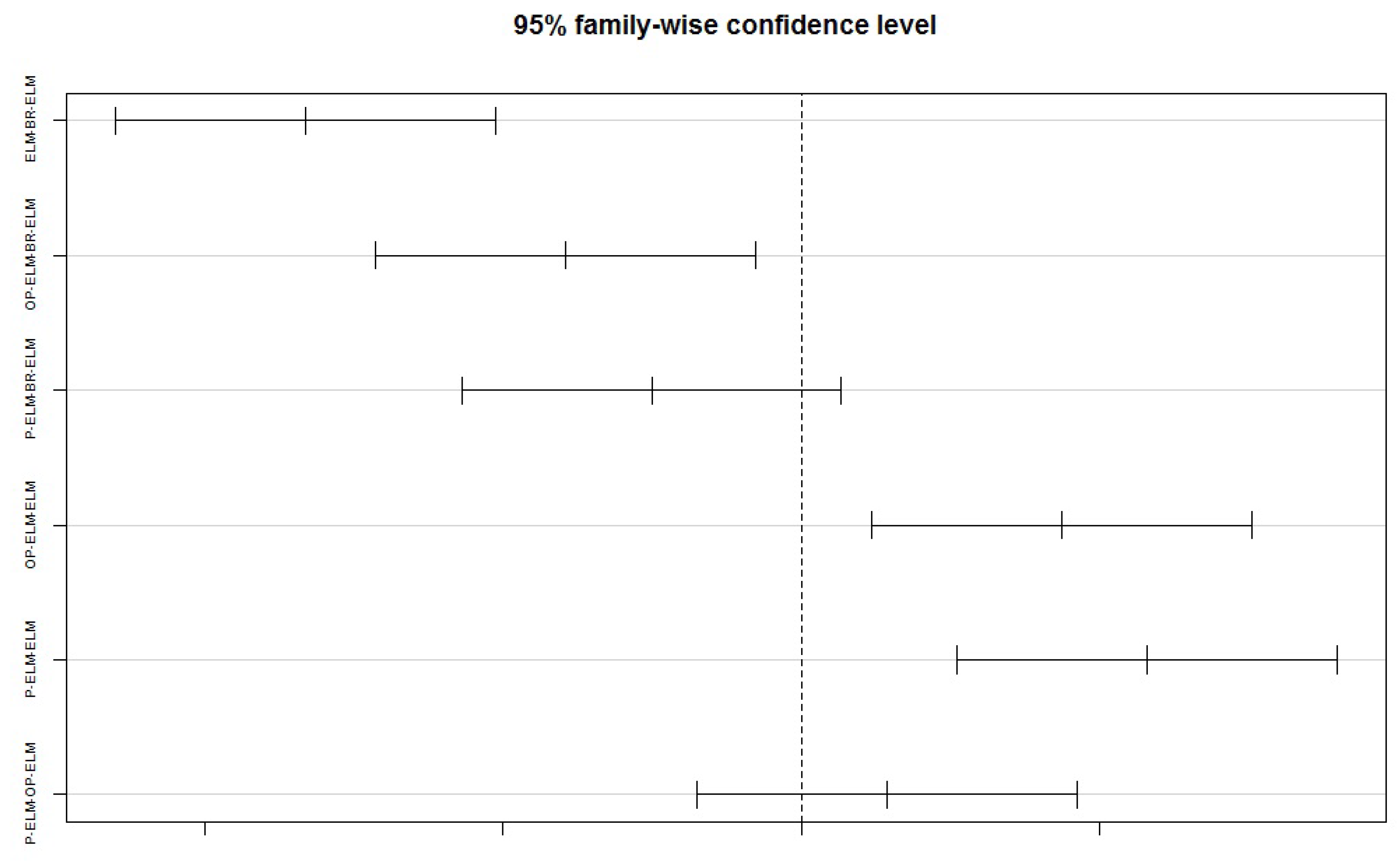
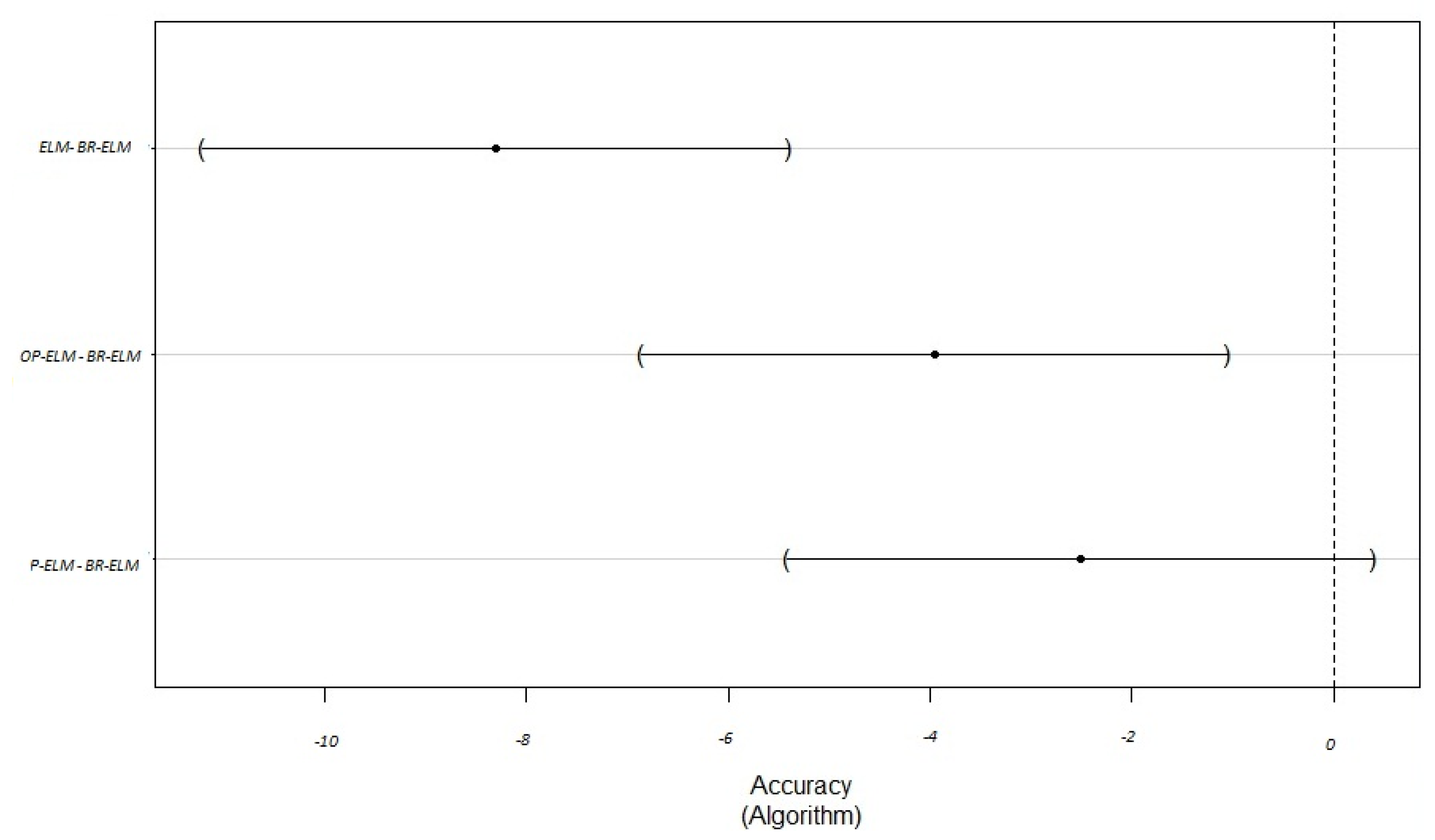
| Algorithm | diff | lwr | upr. | p-adj |
|---|---|---|---|---|
| ELM-BR-ELM | −8.304 | −11.486961 | −5.1212742 | 0.0000001 |
| OP-ELM-BR-ELM | −3.951 | −7.134020 | −0.7683330 | 0.0094658 |
| P-ELM-BR-ELM | −2.512 | −5.695785 | 0.6699022 | 0.1673468 |
| OP-ELM-ELM | 4.352 | 1.170098 | 7.5357846 | 0.0036086 |
| P-ELM-ELM | 5.791 | 2.608333 | 8.9740199 | 0.0000793 |
| P-ELM-OP-ELM | 1.438 | −1.744608 | 4.6210787 | 0.6282214 |
| Algorithm | Estimate | Std. Error | t Value. | Pr (>|t|) |
|---|---|---|---|---|
| ELM-BR-ELM | −8.304 | 1.196 | −6.944 | 0.001 |
| OP-ELM-BR-ELM | −3.951 | 1.196 | −3.304 | 0.00512 |
| P-ELM-BR-ELM | −2.513 | 1.196 | −2.101 | 0.10281 |
| Dataset | Acronym | Feature | Train | Test |
|---|---|---|---|---|
| Air Quality | AIQ | 2 | 192 | 80 |
| Container Crane Controller | CON | 2 | 10 | 5 |
| Carbon Nanotubes | CAR | 5 | 6698 | 2870 |
| Cloud | CLO | 9 | 72 | 36 |
| Absenteeism at work | ABS | 21 | 518 | 222 |
| Combined Cycle Power Plant | CPP | 4 | 6698 | 2870 |
| Abalone | ABA | 8 | 2874 | 1393 |
| Dataset | BR-ELM | OP-ELM |
|---|---|---|
| AIQ | 7.2119 (0.4818) | 4.1136 (0.6284) |
| CON | 0.5552 (0.3863) | 0.9054 (3.2029) |
| CAR | 0.2399 (0.0055) | 4.1892 (0.1252) |
| CLO | 0.0123 (0.0093) | 0.0223 (0.0113) |
| ABS | 14.25 (2.47) | 13.90 (1.64) |
| CPP | 4.4263 (0.3261) | 4.1645 (0.1262) |
| ABA | 0.6598 (0.0179) | 2.2073 (0.0493) |
| Dataset | BR-ELM | OP-ELM |
|---|---|---|
| AIQ | 82.26 (5.77) | 172.66 (8.58) |
| CON | 16.67 (7.50) | 5.00 (0.00) |
| CAR | 74.26 (9.93) | 84.83 (14.65) |
| CLO | 74.26 (11.44) | 80.00 (6.29) |
| ABS | 25.46 (10.41) | 46.33 (14.79) |
| CPP | 107.50 (21.71) | 135.50 (12.95) |
| ABA | 56.33 (8.99) | 55.66 (7.73) |
| Model | Sensibility | Specificity | AUC | Accuracy | Training and Test Time | |
|---|---|---|---|---|---|---|
| BR-ELM | 35.93 (14.13) | 72.99 (3.59) | 87.68 (2.81) | 0.8034 (0.01) | 85.34 (1.60) | 60.01 (4.48) |
| CE-ELM | 99.86 (6.88) | 63.65 (25.66) | 83.91 (8.37) | 0.7420 (0.10) | 74.83 (11.31) | 0.08 (0.03) |
| PS-ELM | 68.64 (16.14) | 71.20 (1.16) | 81.14 (0.98) | 0.7617 (0.12) | 79.23 (1.76) | 54.14 (2.16) |
| ARD-ELM | 71.20 (16.67) | 73.06 (3.92) | 87.03 (2.45) | 0.8005 (0.02) | 81.86 (2.04) | 50.74 (3.87) |
| ELM | 200.00 (0.00) | 65.14 (8.37) | 84.53 (3.31) | 0.7483 (0.03) | 77.36 (2.54) | 0.01 (0.00) |
| Model | Sensibility | Specificity | AUC | Accuracy | Training and Test Time | |
|---|---|---|---|---|---|---|
| BR-ELM | 34.76 (16.80) | 100.0 (0.00) | 97.94 (1.45) | 0.9897 (0.00) | 98.72 (0.92) | 58.85 (3.26) |
| CE-ELM | 99.69 (4.56) | 75.51 (11.12) | 81.85 (34.31) | 0.7936 (0.11) | 76.75 (10.48) | 0.08 (0.04) |
| PS-ELM | 76.42 (5.82) | 98.15 (0.07) | 84.19 (0.14) | 0.9122 (0.04) | 91.18 (0.54) | 63.21 (1.78) |
| ARD-ELM | 111.50 (14.20) | 100.00 (0.00) | 97.82 (0.00) | 0.9891 (0.01) | 98.63 (0.75) | 66.94 (6.61) |
| ELM | 200.00 (0.00) | 94.59 (2.60) | 84.92 (4.46) | 0.8975 (0.02) | 88.46 (2.76) | 0.11 (0.02) |
© 2020 by the authors. Licensee MDPI, Basel, Switzerland. This article is an open access article distributed under the terms and conditions of the Creative Commons Attribution (CC BY) license (http://creativecommons.org/licenses/by/4.0/).
Share and Cite
de Campos Souza, P.V.; Bambirra Torres, L.C.; Lacerda Silva, G.R.; Braga, A.d.P.; Lughofer, E. An Advanced Pruning Method in the Architecture of Extreme Learning Machines Using L1-Regularization and Bootstrapping. Electronics 2020, 9, 811. https://doi.org/10.3390/electronics9050811
de Campos Souza PV, Bambirra Torres LC, Lacerda Silva GR, Braga AdP, Lughofer E. An Advanced Pruning Method in the Architecture of Extreme Learning Machines Using L1-Regularization and Bootstrapping. Electronics. 2020; 9(5):811. https://doi.org/10.3390/electronics9050811
Chicago/Turabian Stylede Campos Souza, Paulo Vitor, Luiz Carlos Bambirra Torres, Gustavo Rodrigues Lacerda Silva, Antonio de Padua Braga, and Edwin Lughofer. 2020. "An Advanced Pruning Method in the Architecture of Extreme Learning Machines Using L1-Regularization and Bootstrapping" Electronics 9, no. 5: 811. https://doi.org/10.3390/electronics9050811
APA Stylede Campos Souza, P. V., Bambirra Torres, L. C., Lacerda Silva, G. R., Braga, A. d. P., & Lughofer, E. (2020). An Advanced Pruning Method in the Architecture of Extreme Learning Machines Using L1-Regularization and Bootstrapping. Electronics, 9(5), 811. https://doi.org/10.3390/electronics9050811