An Advanced CNN-LSTM Model for Cryptocurrency Forecasting

Abstract

Nowadays, cryptocurrencies are established and widely recognized as an alternative exchange currency method. They have infiltrated most financial transactions and as a result cryptocurrency trade is generally considered one of the most popular and promising types of profitable investments. Nevertheless, this constantly increasing financial market is characterized by significant volatility and strong price fluctuations over a short-time period therefore, the development of an accurate and reliable forecasting model is considered essential for portfolio management and optimization. In this research, we propose a multiple-input deep neural network model for the prediction of cryptocurrency price and movement. The proposed forecasting model utilizes as inputs different cryptocurrency data and handles them independently in order to exploit useful information from each cryptocurrency separately. An extensive empirical study was performed using three consecutive years of cryptocurrency data from three cryptocurrencies with the highest market capitalization i.e., Bitcoin (BTC), Etherium (ETH), and Ripple (XRP). The detailed experimental analysis revealed that the proposed model has the ability to efficiently exploit mixed cryptocurrency data, reduces overfitting and decreases the computational cost in comparison with traditional fully-connected deep neural networks.

1. Introduction

Cryptocurrencies have been established and widely recognized as a new electronic alternative exchange currency method, which have considerable implications for emerging economies and in general for the global economy [1]. They have infiltrated most financial transactions and as a result cryptocurrency trade is generally considered one of the most popular and promising type of profitable investments. Nevertheless, this constantly increasing financial market is characterized by significant volatility and strong price fluctuations over time. Nowadays, cryptocurrency forecasting is generally considered as one of the most challenging time-series prediction problems due to the large number of unpredictable factors involved and the significant volatility of cryptocurrencies’ prices, resulting in complicated temporal dependencies [2,3,4].

Over the last years, deep learning methodologies were applied on time-series predictions, focusing on popular real-world application domains such as the cryptocurrency market. Most of these models exploit advanced deep learning techniques and special architectural designs based on convolutional and long short-term memory (LSTM) layers [5,6,7,8,9,10]. Convolutional layers are utilized to filter out the noise in complex time-series data as well as extracting new valuable features while LSTM layers are used to efficiently capture sequence patterns as well as long and short term dependencies [9].

Nevertheless, although advanced deep learning models possess the ability to address highly nonlinear time-series problems, they were proved to produce inefficient and unreliable cryptocurrency forecasts. More specifically, Pintelas et al. [11] and Livieris et al. [12] presented some comprehensive researches and highlighted that the difficulties in cryptocurrency forecasting are based on two main reasons: First, cryptocurrencies time-series are close to random walk process, which implies that the prediction problem is considered too complex and too complicated and second, the inefficiency of deep learning models is mainly based on the existence of autocorrelation in the errors and the lack of stationarity [2,13]. It is worth mentioning that stationarity property constitutes an important property in time-series modeling as well as for the reliability of the prediction models. Notice that non-stationary series possess high volatility, trend, are frequently characterized by heteroskedasticity, and significant properties such as mean, frequency, variance, and kurtosis vary over time.

Along this line, Livieris et al. [2] introduced a novel framework for enhancing deep learning forecasting models. The major novelty of their proposed work was the enforcement of a time-series to become “suitable” for fitting a deep learning model based on the stationarity property, as well as a framework for the development of accurate and reliable prediction models. To impose stationarity the authors performed a series of transformations based on first differences or returns, without the loss of any embedded information. Additionally, they performed extensive research focusing on the evaluation of the prediction accuracy of deep learning models, as well as the reliability of their forecasts by examining the existence of autocorrelation in the errors. Based on their experimental and theoretical evidence, the authors concluded that their proposed framework secures the “suitability” of a time-series for fitting a deep learning model and it is essential for developing accurate and reliable deep learning time-series models.

Based on the previous works, the objective of this research is two-fold: Firstly, to investigate if the forecasting accuracy of a cryptocurrency deep learning model can be indeed enhanced by utilizing data from various cryptocurrencies and secondly, to develop a deep learning model with advanced forecasting accuracy.

In this work, we propose a multiple-input deep neural network model, called MICDL, for the prediction of a cryptocurrency price and movement. Initially, all cryptocurrency time-series data are transformed based on returns transformation in order to satisfy the stationarity property and be “suitable” for fitting the proposed deep neural network model [2]. Subsequently, the proposed prediction model uses as inputs the transformed data from various cryptocurrencies and handles them independently, in the sense that each cryptocurrency data consist of inputs to different convolutional layers, in order for each cryptocurrency information to be exploited and processed, separately. Finally, the processed data from each cryptocurrency are merged and further processed for issuing the final prediction. The rationale for the utilization of a multi-input neural network is that these types of models have been originally proposed for more efficiently exploiting mixed data and refers to the case of having multiple types of independent data [14]. In the literature, these models have been successfully applied for addressing a variety of difficult real-world problems reporting promising results while they were found to outperform traditional single output models [14,15,16,17,18]. The main idea behind these models is to extract valuable information from each category of mixed data, independently and then concatenate the information for issuing the final prediction. Additionally, we conducted an empirical study utilizing almost four consecutive years (1 January 2017–31 October 2020) of cryptocurrency data from the three cryptocurrencies with the highest market capitalization i.e., Bitcoin (BTC), Etherium (ETH), and Ripple (XRP). The numerical experiments report that the proposed model provided reliable price movement predictions outperforming traditional deep learning models as well as accurate price forecasting. Moreover, the detailed experimental analysis highlight that MICDL has the ability to efficiently exploit mixed cryptocurrency data and reduces overfitting with lower computational cost compared to a traditional fully-connected deep neural network.

The remainder of this paper is organized as follows: Section 2 presents a brief review of deep learning models for cryptocurrency price and movement forecasting. Section 3 presents a detailed description of the proposed framework focusing on highlighting its architecture and benefits. Section 4 presents data preparation and reports the descriptive statistics, describing the basic features of each data. Section 5 presents the detailed experimental analysis, focusing on the evaluation of the proposed framework. Section 6 summarizes the main findings of this research, presents the conclusions, and some interesting future directions.

2. Related Work

Cryptocurrency price analysis and forecasting constitutes a considerably complicated problem in time-series analysis and a considerably challenging research area. Its complexity and difficulty is caused by the cryptocurrency time-series’ significant fluctuations and volatility, which are highly influenced by an enormous number of factors. In the literature, recent research efforts have utilized and adopted deep learning methodologies for predicting cryptocurrency price and directional movement to improve forecasting accuracy. Some interesting findings and useful conclusions are briefly presented.

Derbentsev et al. [3] attempted to model short-term dynamics of the three most capitalized cryptocurrencies, i.e., Bitcoin, Etherium, and Ripple, using several sophisticated prediction models. More specifically, they evaluated the prognostic performance of an artificial neural network (ANN), a random forest (RF), and a binary autoregressive tree (BART) model. The utilized data obtained 1583 daily cryptocurrency prices from 1 August 2015 to 1 December 2019. Their experimental results reported that that ANN and BART models exhibited a 63% average accuracy for predicting directional movement which was considerably higher than the “naive” model.

Chowdhury et al. [4] applied advanced machine learning prediction models on the index and constituents of cryptocurrencies for forecasting future values. More analytically, their primary aim was the prediction of the closing price of the CCI30 index as well as nine major cryptocurrencies in order to assist cryptocurrency investors in trading. In their work, they utilized a variety of machine learning models including gradient boosted trees, ANNs, k-nearest neighbor, as well as robust ensemble learning models. Their utilized data contained daily closing prices from 1 January 2017 to 31 January 2019. Ensemble models and gradient boosted trees exhibited the best prediction performance, which was competitive and sometimes better, compared to that of similar state-of-the-art models proposed in the literature.

Pintelas et al. [11] conducted interesting research, evaluating sophisticated deep learning models for predicting cryptocurrency prices and movements. Their research revealed the significant limitations of deep learning models for exhibiting reliable forecasts. Based on their experimental analysis, the authors highlighted the need for adopting more advanced algorithmic approaches for the development of efficient and reliable cryptocurrency models. Along this line, Livieris et al. [12] considered improving the forecasting performance and reliability of deep learning models utilizing three widely utilized ensemble strategies, i.e., averaging, bagging, and stacking. The authors utilized hourly prices of Bitcoin, Etherium, and Ripple from 1 January 2018 to 31 August 2019. Additionally, they conducted an exhaustive performance evaluation of various ensemble models using several Conv-based and LSTM-based learners as base models. Their analysis highlighted that deep learning and ensemble learning may efficiently be adapted to develop strong, and reliable cryptocurrency prediction models, but with significant computational cost.

Patel et al. [19] proposed a hybrid cryptocurrency prediction approach, which focuses on Litecoin and Monero cryptocurrencies. The proposed model is based on a recurrent neural network architecture which utilizes LSTM and GRU layers. The data in their study contained daily Litecoin data from 24 August 2016 to 23 February 2020 and Monero data from 30 January 2015 to 23 February 2020 concerning average price, open price, close price, high and low prices, as well as the volume of trades. The reported experiments demonstrated that the proposed hybrid model outperforms traditional LSTM networks exhibiting some promising results.

A common limitation of all presented and discussed researches is that they focused on achieving better forecasting performance by exploiting more sophisticated models and techniques, usually ignoring the development of a sophisticated training dataset containing more useful information. In other words, most approaches treat each cryptocurrency independently ignoring its conceivable relations with other cryptocurrencies and do not take into consideration the complexity and non-stationarity of cryptocurrency time-series data.

In this research, we propose a different approach and present a new model for the development of accurate and reliable forecasting models. The novelty of the proposed model is based on the utilized training data as well as its special architectural design. More specifically, in this work, we propose a multiple-input deep neural network model, which utilizes as inputs various cryptocurrency data and handles them independently in order to each cryptocurrency information to be exploited and processed, separately. The processed data from each cryptocurrency are merged and further processed for issuing the final prediction. To the best of our knowledge this is the first conducted approach that has focused exploit data from various cryptocurrencies for exhibiting more accurate forecasts. Following previous approaches [11,12], we provide a comprehensive performance evaluation for price prediction and directional movement.

3. Multiple-Input Cryptocurrency Deep Learning Model

In this section, we present the proposed MICDL model. The proposed approach is based on the idea of not prossessing all cryptocurrency data, simultaneously. In contrast, each cryptocurrency data is processed and handled independently and then the processed data from each cryptocurrency are merged and further processed for estimating the final prediction. The rationale behind the proposed approach is to develop a learning model which is able to independently extract useful information from various cryptocurrency data and subsequently process these information for achieving accurate and reliable predictions.

Suppose that we have data from N cryptocurrencies. Each cryptocurrency data is utilized as input in a unique convolutional layer, which is followed by a pooling layer and a LSTM layer. The proposed approach focuses on exploiting the ability of convolutional layers for extracting useful knowledge by learning the internal representation of each cryptocurrency, independently, as well as the effectiveness of LSTM layers for identifying short-term and long-term dependencies. Then, the output vectors of all LSTM layers are merged by a concatenate layer. This layer is followed by a series of layers, which constitute the classical structure of a deep learning neural network i.e., a dense layer, a batch normalization layer, a dropout layer, a dense layer, a batch normalization layer, a dropout layer, and a final output layer of one neuron. The architecture of MICDL is presented in Figure 1.

Notice that although a traditional deep neural network model is able to analyze and encode any complex function, the convergence of its training process may be degradated due to the number of weights, which exponentially increases as the number of layers increases and due to the vanishing gradient problem, which usually occurs in large networks. In contrast, the significant advantages of the proposed model’s architecture is that it provides more flexibility and adaptivity for low computation effort compared to a fully connect neural network with a similar number of layers as well as greater resistance to the vanishing gradient problem, due to its sparse structure [16,20].

Subsequently, we present a brief description of the main elements of the proposed MICRL model i.e., convolution and pooling layers, LSTM layers, dense layers, batch-normalization layers, and dropout layers.

• Convolutional layer: Convolutional layers [21] constite a novel class of neural network layers which are characterized by their remarkable ability to learn the internal representation of their inputs. This is performed by applying convolutional operations between the input data and the use of convolution kernels, called “filters”, for developing new feature values;
• Pooling layer: Pooling layers [21] are utilized to reduce the spatial dimensions, aiming to reduce the number of operations required for all following layers. Notice that less spatial information implies less weights, so less chance to overfit the training data and less computional effort. In more detail, these layers are utilized to downsample the output of a previous layer, which is usually a convolutional layer, attempting to pass only valid and useful information. Probably, max pooling and average pooling layers constitute the most widely utilized choices, which use the maximum value and the average value from each cluster of outputs of the previous layer, respectively [22];
• LSTM layer: LSTM layers [23] belong to the class of recurrent neural network layers, enhanced with a separate memory cell and adaptive gate units (input, forget, and output) for controlling the information flow. The utilization of gates in each cell implies that data can be filtered, discarded, or added therefore maintaining useful information in the memory cell for longer periods of time. The advantage of LSTM layers are their ability to identify both short and long term correlation features within time series and considerably address the vanishing gradient problem [23];
• Dense layer: Dense layers constitute the most popular and widely utilized choice for composing the hidden layer of a deep neural network [24]. In particular, each dense layer is composed by neurons, which are connected with all neurons of the previous layer. Generally, dense layers add a non-linearity property and theoretically a neural network composed by dense layers is able to model any mathematical function [25];
• Batch-normalization layer: Batch normalization constitutes an elegant technique for training deep neural networks which focuses on stabilizing the learning process by standardizing the inputs of the next layer for each mini-batch [21]. Batch normalization significantly reduces the problem of coordinating updates across many layers and usually accelerates training by considerably reducing the number of epochs;
• Dropout layer: Dropout constitutes one of the most famous regulization methods for preventing neural-networks from overfitting. The dropout layer is a non-learnable layer which is added between existing layers of a neural network model. It is applied to outputs of the prior layer and temporarily sets a random set of outputs to zero with a pre-defined probability p, called the dropout rate, which are fed to the next layer. The key idea in dropout and its motivation is to make each layer less sensitive to statistical fluctuations in the inputs [26].

4. Data

The data utilized in this research, concern daily historical data from 1 January 2017 to 31 October 2020 of BTC, ETH, and XRP in USD, which constitute the cryptocurrencies with the highest market capitalization. Moreover, the data for all cryptocurrencies were collected from the website https://coinmarketcap.com.

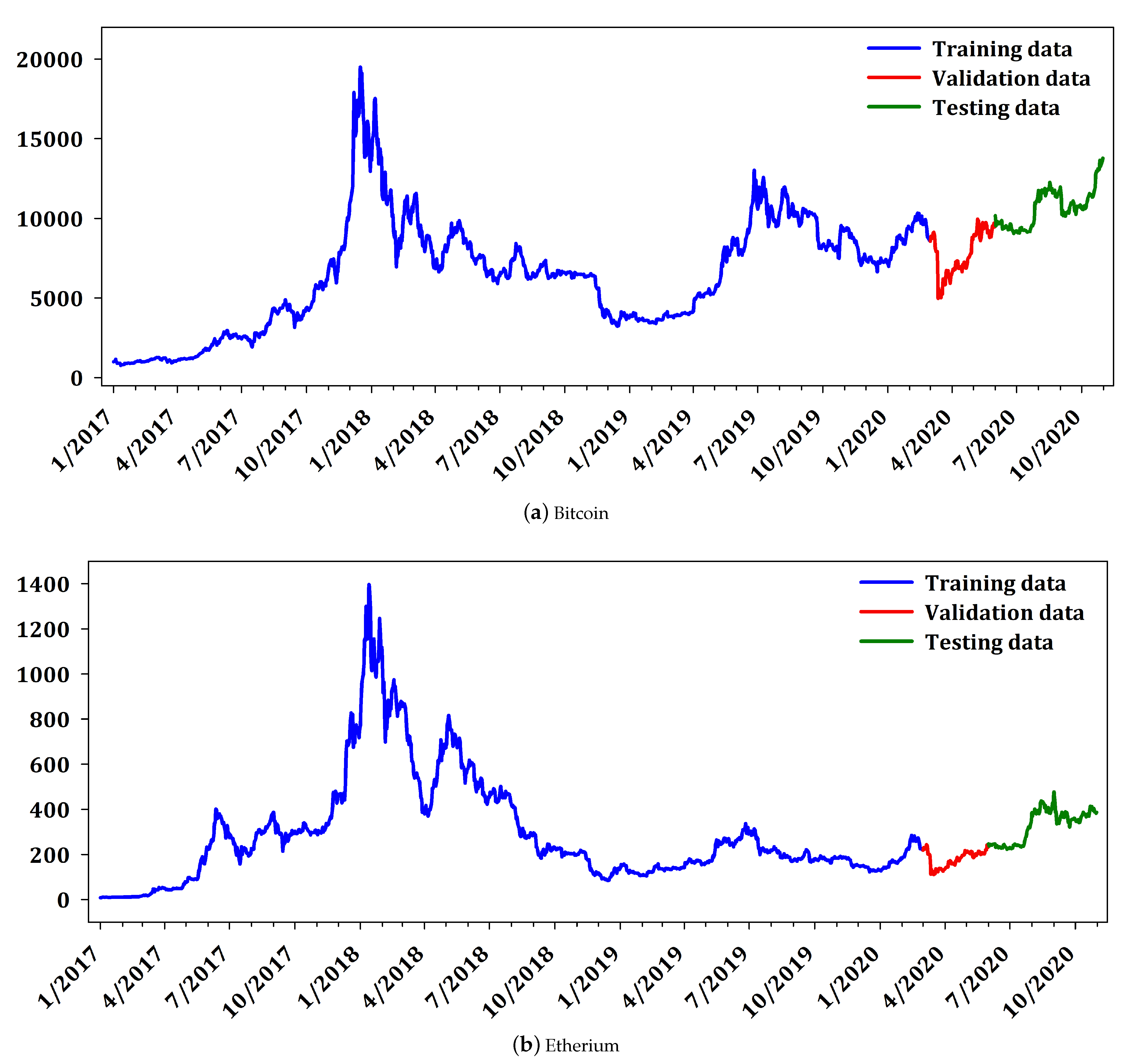
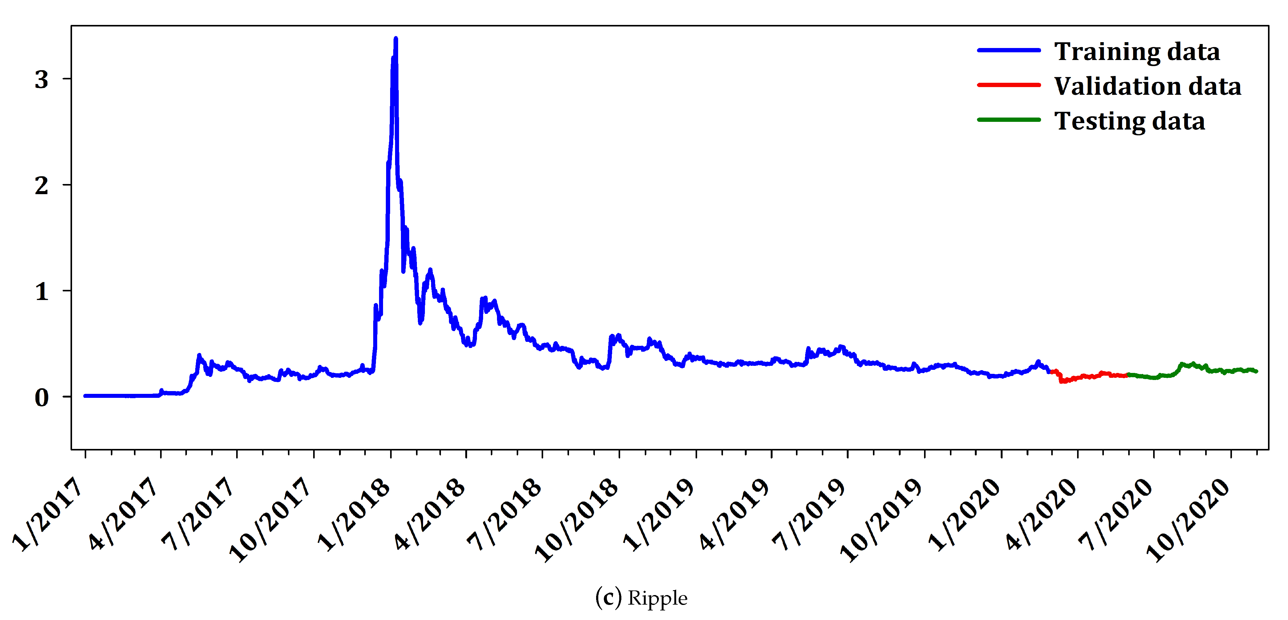
For evaluation purposes, the cryptocurrency data were divided in training set, validation set, and testing set. More analytically the training set comprised of daily data from 1 January 2017 to 18 February 2020 (1153 datapoints), the validation set from 1 March 2020 to 31 May 2020 (94 datapoints) while the testing set consisted of data from 1 June 2020 to 31 October 2020 (152 datapoints) which ensured a considerable amount of unseen out-of-sample datapoints for testing. Finally, it is worth noticing that all utilized datasets contained values that include the recent COVID-19 crisis in the beginning of 2020, which are characterized by considerable volatility and deviations from the regular behavior as well as structural breaks.

Figure 2 presents the daily price of the cryptocurrencies BTC, ETH, and XRP. The interpretation of Figure 2 reveals that Ripple does not have large variability as Bitcoin and Etherium. It is worth mentioning that Ripple constitutes a different cryptocurrency, from the point of view that it is not mineable, it is pre-mined, and it has small variability compared to the other two cryptocurrencies. Nevertheless, since Ripple is highly ranked in market capitalization, it is traditionally included in most research works in cryptocurrency market. Furtermore,

Table 1. Descriptive statistics for BTC, ETH, and XRP data.

Data		Minimum	Maximum	Mean	Std. Dev.	Median	Skewness	Kurtosis
BTC	Training set	777.76	19,497.40	6459.19	3496.35	6588.31	0.44	0.26
	Validation set	4970.79	9951.52	7810.27	1358.18	7801.33	−0.25	−1.08
	Testing set	9045.39	13,780.99	10,663.35	1178.23	10,680.84	0.47	−0.46
ETH	Training set	8.17	1396.42	291.33	240.22	217.05	1.71	3.03
	Validation set	110.61	243.53	181.16	35.93	192.09	−0.35	−1.12
	Testing set	222.96	477.05	328.80	71.57	353.21	−0.26	−1.44
XRP	Training set	0.01	3.38	0.39	0.36	0.30	3.68	19.98
	Validation set	0.14	0.24	0.19	0.02	0.20	−0.23	−0.26
	Testing set	0.18	0.31	0.24	0.04	0.24	0.15	−1.00

illustrates the descriptive statistics including mean, median, maximum, minimum, standard deviation (std. dev.), skewness, and kurtosis for each cryptocurrency and CCi30 index while

Table 2. The number of up and down movements of BTC, ETH, and XRP data.

Data		Up		Down
BTC	Training set	630	54.74%	521	45.26%
	Validation set	50	53.76%	43	46.24%
	Testing set	87	57.24%	65	42.76%
ETH	Training set	577	50.22%	572	49.78%
	Validation set	51	54.84%	42	45.16%
	Testing set	85	55.92%	67	44.08%
XRP	Training set	538	46.74%	613	53.26%
	Validation set	52	55.91%	41	44.09%
	Testing set	80	52.63%	72	47.37%

summarizes the up and down movements in the prices and the corresponding percentages.

Next, following the novel framework, which was originally proposed by Livieris et al. [2] all cryptocurrency data are initially transformed based on the returns transformation in order to satisfy the stationarity property and to be “suitable” for fitting a deep neural network model.

Table 3. Augmented Dickey–Fuller (ADF) unit root test of all cryptocurrency time-series.

Time-Series		t-Statistic	p-Value
Levels	BTC	−1.831855	0.364765
	ETH	−2.058319	0.261601
	XRP	−3.880291	0.002185
Transformed	BTC	−36.832969	0.000000 *
	ETH	−36.832969	0.000000 *
	XRP	−36.832969	0.000000 *

reports the t-statistics and the associated p-values of the augmented Dickey–Fuller (ADF) test [27,28] performed on the level (Levels) of the cryptocurrency series as well as of the corresponding transformed time-series. Notice that (∗) denotes statistical significance at the 5% critical level. The interpretation of Table 3 reveals that BTC, ETH, and XRP time-series possess a unit root which implies that these series are non-stationary. Additionally, the corresponding p-value of the transformed series are practically zero, which denotes that they satisfy the stationarity property and are “suitable” fitting a deep learning model.

Finally, it is worth noticing that all deep learning models were trained using the transformed series and the inverse transformations were applied for calculating the prediction for the levels of the original time-series.

5. Numerical Experiments

In this section, we conducted extensive experimental analysis to examine and evaluate the performance of proposed multi-input deep learning model in forecasting the cryptocurrency prices of Bitcoin, Etherium, and Ripple.

The proposed model was evaluated against two CNN-LSTM models: Model${}_1$ and Model${}_2$. Model${}_1$ is trained with only one cryptocurrency data (i.e., BTC, ETH, or XRP), while Model${}_2$ is trained with all three cryptocurrency data, as well as the proposed MICDL model.

• Model${}_1$ consists of a convolutional layer of 16 filters of size $(2;)$, followed by an average pooling layer of size 2, a LSTM layer of 50 units, a batch normalization layer a dropout out layer with $p=0.4$, a dense layer of 64 neurons, a batch normalization layer a dropout out layer with $p=0.2$, and an output layer of one neuron;
• Model${}_2$ consists of a convolutional layer of 32 filters of size $(2;)$, followed by an average pooling layer of size 2, a LSTM layer of 50 units, a batch normalization layer a dropout out layer with $p=0.5$, a dense layer of 128 neurons, a batch normalization layer a dropout out layer with $p=0.2$, and an output layer of one neuron;
• MICDL model consists of 3 convolutional layers with 16 filters of size $(2;)$, each one takes as input a unique cryptocurrency time-series data, i.e., BTC, ETH, and XRP. Each convolutional layer is followed by am average pooling layer of size $(2;)$ and a LSTM layer with 50 units. The outputs of the LSTM layers are merged by a concatenate layer which is followed by a dense layer of 256 neurons, a batch normalization layer, a dropout layer with $p=0.3$ a dense layer of 64 neurons, a batch normalization layer, a dropout layer with $p=0.2$, and a final output layer of one neuron.

Each cryptocurrency prediction model was trained utilizing two different Lag values i.e., 7 (1 week) and 14 (2 weeks) while their hyper-parameters were optimized under exhaustive experimentation (used various number of filters in convolutional layers, units in LSTM layers, neurons in dense layers, and values of dropout rate).

For evaluating the regression performance of all forecasting models we utilized the performance metrics: mean absolute error (MAE), root mean square error (RMSE), and coefficient of determination $R^2$, which are respectively defined by:

$$\begin{array}{ccc}\hfill \mathrm{MAE}& =& \frac{1}{N}\sum _{t=1}^N|y_t-{\widehat{y}}_t|\hfill \\ \hfill \mathrm{RMSE}& =& \sqrt{\frac{1}{N}\sum _{t=1}^N{(y_t-{\widehat{y}}_t)}^2}\hfill \\ \hfill R^2& =& 1-\frac{{\displaystyle \sum _{t=1}^N{(y_t-{\widehat{y}}_t)}^2}}{{\displaystyle \sum _{t=1}^N{(y_t-\overline{y})}^2}}\hfill \end{array}$$

where N is the number of forecasts, $y_t$ is the actual value, ${\widehat{y}}_t$ is the predicted value, and $\overline{y}=\frac{1}{n}{\sum }_{t=1}^N{y}_t$ is the mean of the actual values.

Furthermore, for the binary classification problem of directional movement (price increasement or decreasement on the following day with respect to the today’s price), we utilized the metrics: Accuracy (Acc), Geometric Mean (GM), Sensitivity (Sen), and Specificity (Spe), which are respectively defined by:

$$\begin{array}{ccc}\hfill \mathrm{Acc}& =& \frac{\mathrm{TP}+\mathrm{TN}}{\mathrm{TP}+\mathrm{FP}+\mathrm{FN}+\mathrm{FP}}\hfill \\ \hfill \mathrm{GM}& =& \sqrt{\mathrm{TP}·\mathrm{TN}}\hfill \\ \hfill \mathrm{Spe}& =& \frac{\mathrm{TP}}{\mathrm{TP}+\mathrm{FN}}\hfill \\ \hfill \mathrm{Spe}& =& \frac{\mathrm{TN}}{\mathrm{TN}+\mathrm{FP}}\hfill \end{array}$$

where TP stands for the number of values which were correctly identified to be increased, TN stands for the number of values which were correctly identified to be decreased, FP (type I error) stands for the number of values which were misidentified to be increased, and FN (type II error) stands for the number of values which misidentified to be decreased.

Moreover, the performance metric area under curve (AUC) was included in our experimental analysis which is presented using the receiver operating characteristic (ROC) curve. Notice that ROC curve is created by plotting the true positive rate (Sensitivity) against the false positive rate (Specificity) at various threshold settings.

All models were trained with root mean square propagation (RMSProp) [29]. The rectifier linear unit (ReLU) activation function was utilized as an activation function except for the output layer where the linear activation was used. In all layers, the kernel and bias initializer were set as default as well as the recurrent initializer in the LSTM layers. Additionally, in order to avoid overfitting we used the early stopping technique based on “validation loss”.

At this point, it is worth mentioning that the performance metrics AUC and GM as well as the balance between Sen and Spe present the information provided by a confusion matrix in compact form hence, they constitute the proper metrics to evaluate the ability of model of not overfitting the training data.

Table 4. Performance of the evaluated models for all BTC data.

Model	Lag	MAE	RMSE	${\mathit{R}}^2$	Accuracy	AUC	GM	Sen	Spe
Model${}_1$	7	169.817	256.688	0.953	55.03%	0.494	20.058	0.881	0.108
Model${}_2$		169.604	256.318	0.953	53.64%	0.497	26.567	0.770	0.224
MICDL		170.761	257.728	0.952	53.04%	0.502	30.886	0.698	0.306
Model${}_1$	14	171.292	262.339	0.950	53.53%	0.504	27.962	0.720	0.288
Model${}_2$		170.105	256.849	0.952	52.60%	0.506	23.727	0.645	0.367
MICDL		171.147	257.847	0.952	51.88%	0.508	29.173	0.582	0.434

,

Table 5. Performance of the evaluated models for all ETH data.

Model	Lag	MAE	RMSE	${\mathit{R}}^2$	Accuracy	AUC	GM	Sen	Spe
Model${}_1$	7	9.172	13.517	0.964	51.51%	0.495	25.770	0.666	0.324
Model${}_2$		9.302	13.591	0.964	48.85%	0.498	23.961	0.419	0.576
MICDL		9.233	13.551	0.964	50.86%	0.504	29.582	0.483	0.526
Model${}_1$	14	9.309	13.657	0.964	49.57%	0.482	27.888	0.596	0.369
Model${}_2$		9.196	13.539	0.964	50.38%	0.503	27.930	0.513	0.492
MICDL		9.146	13.492	0.964	51.11%	0.495	30.461	0.628	0.363

and

Table 6. Performance of the evaluated models for all XRP data.

Model	Lag	MAE	RMSE	${\mathit{R}}^2$	Accuracy	AUC	GM	Sen	Spe
Model${}_1$	7	0.005	0.007	0.960	48.97%	0.497	22.031	0.348	0.646
Model${}_2$		0.005	0.007	0.958	49.61%	0.497	22.274	0.475	0.520
MICDL		0.005	0.007	0.958	49.07%	0.498	25.053	0.366	0.630
Model${}_1$	14	0.005	0.007	0.962	49.34%	0.499	22.418	0.391	0.607
Model${}_2$		0.006	0.009	0.936	49.23%	0.501	23.351	0.340	0.662
MICDL		0.007	0.009	0.953	49.23%	0.495	26.157	0.442	0.549

summarize the performance of all forecasting models, based on BTC, ETH, and XRP data, respectively. Clearly, all model exhibited similar performance, regarding the performance metrics MAE, RMSE, and $R^2$. By comparing the performance of Model${}_2$ and MICDL with the performance of Model${}_1$, we can easily conclude that the utilization of all three series in the training data did not developed a forecasting model with better regression performance. More specifically, all models reported an almost identical regression performance.

In contrast, regarding the classification problem of forecasting the price movement both MICDL and Model${}_2$ considerably outperformed Model${}_1$, regarding all Lag values and cryptocurrencies. More specifically, for Lag value 7, Model${}_1$ reported 20.058, 25.77, and 22.031 GM score for BTC, ETH, and XRP while Model${}_2$ reported 26.567, 23.961, and 22.274, and MICDL reported 30.886, 29.582, and 25.053 in the same situations. Regarding Lag value 14, Model${}_1$ exhibited 27.962, 27.888, and 22.418 a GM score for BTC, ETH, and XRP while Model${}_2$ exhibited 23.727, 27.930m and 23.351 and MICDL exhibited 29.173, 30.461, and 26.157 in the same situations. Additionally, both MICDL and Model${}_2$ reported a better balance between Sen and Spe metrics compared to Model${}_1$, regarding all cryptocurrencies and Lag values. Finally, it is worth mentioning, that Model${}_1$ and Model${}_2$ reported better classification performance for Lag value 14, while MICDL reported similar performance for both Lag values.

The interpretation of Table 4, Table 5 and Table 6 show that Model${}_1$ has overfitted the training data and it is not able to make reliable price movement predictions which implies that the utilization of all cryptocurrencies in the training data has benefitted the development of prediction models with better classification performance. Additionally, by comparing the performance of the proposed model MICDL with that of Model${}_2$, we point out that the special architecture of MICDL has better exploited the training data and is able to predict price movements with higher accuracy and reliability. Finally, it is worth mentioning that MICDL considerably outperformed both Model${}_1$ and Model${}_2$ reporting 12.5–54% and a 4.33–22.95% higher GM score for Lag values 7 and 14, respectively as well as presenting the best balance between Sen and Spe metrics.

Based on the previous analysis, we are able to conclude that the utilization of all cryptocurrencies in the training data but most significantly the multi-input architecture of the proposed MICDL has developed a forecasting model with the best regression and classification performance. Although the $R^2$ metric presents that all models have equally fitted the training data and are able to exhibit accurate cryptocurrency predictions, the metrics GM, Sen, and Spe reveal that the utilization of all series in the training data provided models with improved performance regarding the directional movement problem. This indicates that although Model${}_1$ is able to predict a value close to the next value, it cannot provide any reliable information if the cryptocurrency price will increase or decrease the next day. Moreover, the architecture of the MICDL model developed a model which has efficiently exploited the information provided in the training set and is able to provide accurate and reliable price movement prediction without degradating its regression performance.

Next, we attempt to provide statistical evidences about the efficiency and reliability of the proposed MICDL model’s forecasts. In more detail, for rejecting the hypothesis $H_0$ that all cryptocurrency models performed equally well for a given level, we utilized the non-parametric Friedman aligned ranking (FAR) [30] test. In addition, in order to examine if the differences in the performance of the models are statistically significant, we applied the post-hoc Finner test [31] with significance level $\alpha =5\%$.

Table 7. Friedman aligned ranking (FAR) test and Finner post hoc test based on the mean absolute error (MAE) metric.

Series	Friedman	Finner Post-Hoc Test
	Ranking	p-Value	${\mathit{H}}_0$
MICDL	11.5	−	−
Model${}_2$	7.167	0.29398	accepted
Model${}_1$	9.833	0.38694	accepted

,

Table 8. FAR test and Finner post hoc test based on the root mean square error (RMSE) metric.

Series	Friedman	Finner Post-Hoc Test
	Ranking	p-Value	${\mathit{H}}_0$
Model${}_2$	8.4167	−	−
MICDL	9.4167	0.745603	accepted
Model${}_1$	10.667	0.71420	accepted

and

Table 9. FAR test and Finner post hoc test based on the $R^2$ metric.

Series	Friedman	Finner Post-Hoc Test
	Ranking	p-Value	${\mathit{H}}_0$
Model${}_1$	8.0833	−	−
MICDL	9.5	0.587788	accepted
Model${}_2$	10.9167	0.645784	accepted

report the statistical analysis, performed by nonparametric multiple comparison, relative to MAE, RMSE, and $R^2$ performance metrics. Regarding the regression performance of the evaluated models similar conclusions can be made with the previous analysis. More specifically, the interpretation of Table 7, Table 8 and Table 9 reveals that all models performed equally well, since the differences in their regression performance is not significantly significant.

In sequel, for examining the superiority of MICDL, regarding the problem of predicting future cryptocurrency directional movement, we conduct a nonparametric multiple comparison relative to AUC and GM metrics. Additionally, to measure the difference in the balance of Sen and Spe metrics, we utilize a new metric defined as the product of these two metrics, i.e., Sen × Spe. It is worth noticing that AUC, GM, and Sen × Spe metrics evaluate the ability of model of not overfitting the training data hence, presenting the information provided by a confusion matrix in compact form.

Table 10. FAR test and Finner post hoc test based on the area under curve (AUC) metric.

Series	Friedman	Finner Post-Hoc Test
	Ranking	p-Value	${\mathit{H}}_0$
MICDL	6.917	−	−
Model${}_2$	8.250	0.66531	accepted
Model${}_1$	13.333	0.07332	reject

,

Table 11. FAR test and Finner post hoc test based on the GM metric.

Series	Friedman	Finner Post-Hoc Test
	Ranking	p-Value	${\mathit{H}}_0$
MICDL	3.500	−	−
Model${}_2$	12.500	0.006989	reject
Model${}_1$	12.500	0.006989	reject

and

Table 12. FAR test and Finner post hoc test based on the Sen × Spe metric.

Series	Friedman	Finner Post-Hoc Test
	Ranking	p-Value	${\mathit{H}}_0$
MICDL	3.500	−	−
Model${}_1$	11.833	0.006857	reject
Model${}_2$	13.167	0.003419	reject

present the statistical analysis, performed by nonparametric multiple comparison, relative to AUC, GM, and Sen × Spe metrics. More specifically, the interpretation of Table 10, Table 11 and Table 12 provides statistical evidence that MICDL outperformed both Model${}_1$ and Model${}_2$ and provides more reliable forecasts.

6. Discussion, Conclusions, & Future Research

In this research, we proposed a deep neural network model based on a multi-input archtecture for the prediction of cryptocurrency price and movement. The proposed prediction model uses as inputs cryptocurrency data which handles them independently in order for each cryptocurrency information to be initially exploited and processed, separately. More specifically, each cryptocurrency data consists of inputs to different convolutional and LSTM layers which are utilized for learning the internal representation and identifying short-term and long-term dependencies of each cryptocurrency, respectively. Next, the model merges the processed data obtained from the output vectors of LSTM layers and further process them for making the final prediction. It is worth noticing that all utilized cryptocurrency time-series were transformed based on returns transformation in order to satisfy the stationarity property and be “suitable” for fitting the proposed model.

We conducted a coprehensive experimental analysis using a sufficient amount of cryptocurrency data from the three cryptocurrencies with the highest market capitalization i.e., Bitcoin, Etherium, and Ripple. The detailed experimental analysis highlighted that the proposed model has the ability to efficiently exploit mixed cryptocurrency data, reduce overfitting and secure lower computational cost compared to a traditional fully-connected deep neural network in terms of lower number of weights (and consequently less computational time).

Based on the experimental analysis, we are able to conclude that the utilization of all cryptocurrencies in the training data but most significantly the multi-input architecture of the proposed MICDL developed a forecasting model with the best regression and classification performance. It is worth taking into consideration that although the regression metrics reported that all models are equivalent based on their performance which has been also statistically confirmed, in practice they are not. The classification metrics, especially GM and Sen × Spe, highlighted that the utilization of all cryptocurrency data, could assist the development of prediction models which exhibit better directional movement prediction and that the architecture of proposed model has efficiently exploited the information provided in the training data and is able to provide accurate and reliable price and movement predictions.

A common limitation of traditional approaches is that they focused on achieving better forecasting performance by exploiting more sophisticated models and techniques, usually ignoring the development of a sophisticated training dataset containing more useful information. In more detail, they do not treat each cryptocurrency independently, ignoring its conceivable relations with other cryptocurrencies and do not take into consideration the complexity and non-stationarity of cryptocurrency time-series data. In this research, we proposed a different approach and also presented a new methodology for the development of accurate and reliable forecasting models.

It is worth mentioning that cryptocurrency investors and financial researchers are more interested in the future cryptocurrency price movements rather than knowing the exact future price for making proper investment decisions [2,11]. By taking into consideration that the directional movement prediction problem is of higher significance than the price prediction problem, we can conclude that the proposed model is generally preferable for supporting policy decision-making and cryptocurrency markets behavior.

During the last decade, machine learning and deep learning have been widely adopted for assisting financial researchers and cryptocurrency investors in decision support and portfolio management. Nevertheless, a natural question which rises is “how the widespread adoption of prediction models would feedback into future predictions?” Currently, cryptocurrencies follow a random walk process [2,11,12] however, the increasing usage of prediction models may possibly change the behavior of cryptocurrencies in the future. In other words, the increasing dependency of investors on forecasting model predictions for portfolio optimization will ultimately result in affecting investors’ decisions and cryptocurrencies’ fluctuations and prices.

In addition, the utilized cryptocurrencies in this research were selected because they constitute the cryptocurrencies with the highest market capitalization. As a result, the proposed work should be considered as a first approach for obtaining better forecasting performance, regarding future cryptocurrency prediction. Clearly, the proposed methodology could be extended with the adoption of more cryptocurrencies. Such an extension with more cryptocurrencies could introduce new criteria, which may conceivably influence and improve the forecasting performance thus more experiments are certainly needed and this is our major concern for future research. Moreover, one significant issue which we should also be thoroughly investigate in the future is the adoption of cryptocurrency information such as average daily price, open daily price, close daily price, high and low daily prices, as well as the daily volume of trades or even economic and technical trading indicators [32,33]. However, the rising questions of “which cryptocurrencies are more correlated” and “which features have greater impact in price prediction” are still under consideration. Furthermore, another interesting direction for future research could be the evaluation of the proposed model on high-frequency data.

Finally, since our experiments are quite encouraging, a promising idea is to enhance the propose MICDL model with sophisticated pre-processing techniques based on moving average and exponential smoothing.