Article

Optimizing the Performance of Breast Cancer Classification by Employing the Same Domain Transfer Learning from Hybrid Deep Convolutional Neural Network Model

1
Faculty of Science & Engineering, Queensland University of Technology, Brisbane, QLD 4000, Australia
2
Al-Nidhal Campus, University of Information Technology & Communications, Baghdad 00964, Iraq
3
College of Computer Science and Information Technology, University of Sumer, Thi Qar 64005, Iraq
4
School of Engineering, Manchester Metropolitan University, Manchester M1 5GD, UK
5
Faculty of Electrical Engineering and Computer Science, University of Missouri, Columbia, MO 65211, USA
*
Author to whom correspondence should be addressed.
Electronics 2020, 9(3), 445; https://doi.org/10.3390/electronics9030445
Submission received: 24 January 2020 / Revised: 27 February 2020 / Accepted: 4 March 2020 / Published: 6 March 2020
(This article belongs to the Special Issue Deep Learning for Medical Images: Challenges and Solutions)

Abstract

:
Breast cancer is a significant factor in female mortality. An early cancer diagnosis leads to a reduction in the breast cancer death rate. With the help of a computer-aided diagnosis system, the efficiency increased, and the cost was reduced for the cancer diagnosis. Traditional breast cancer classification techniques are based on handcrafted features techniques, and their performance relies upon the chosen features. They also are very sensitive to different sizes and complex shapes. However, histopathological breast cancer images are very complex in shape. Currently, deep learning models have become an alternative solution for diagnosis, and have overcome the drawbacks of classical classification techniques. Although deep learning has performed well in various tasks of computer vision and pattern recognition, it still has some challenges. One of the main challenges is the lack of training data. To address this challenge and optimize the performance, we have utilized a transfer learning technique which is where the deep learning models train on a task, and then fine-tune the models for another task. We have employed transfer learning in two ways: Training our proposed model first on the same domain dataset, then on the target dataset, and training our model on a different domain dataset, then on the target dataset. We have empirically proven that the same domain transfer learning optimized the performance. Our hybrid model of parallel convolutional layers and residual links is utilized to classify hematoxylin–eosin-stained breast biopsy images into four classes: invasive carcinoma, in-situ carcinoma, benign tumor and normal tissue. To reduce the effect of overfitting, we have augmented the images with different image processing techniques. The proposed model achieved state-of-the-art performance, and it outperformed the latest methods by achieving a patch-wise classification accuracy of 90.5%, and an image-wise classification accuracy of 97.4% on the validation set. Moreover, we have achieved an image-wise classification accuracy of 96.1% on the test set of the microscopy ICIAR-2018 dataset.

1. Introduction

Around the world, breast cancer annually affects about 1.7 million women. Compared to other types of cancer, it is the highest recurrent cause of death [1]. Based on collected data by the American Cancer Society [2], approximately 268,600 new cases were diagnosed as invasive breast cancer patients in 2019. In the same year, there were approximately 62,930 new cases of in-situ breast cancer identified, with roughly 41,760 expected death cases due to breast cancer. Early diagnosis of breast cancer is significant as a means to boost the number of survivors. The high cost of breast cancer diagnosis and high morbidity have motivated researchers to explore solutions to develop more precise models for cancer diagnosis.
In general, malignant (cancerous) and benign (non-cancerous) are the two major types of tumors. The type of tumor is decided based on a variety of cell features. Both of them have their own sub-types and properties. Benign is often not harmful to health, and in most cases, it could not be recognized as cancer. But it can be defined as a small variation in the tissue structure of the breast. Malignant tumors are further classified into two types in situ or invasive. In the case of in-situ carcinoma, cancer cells are restrained inside the ducts or lobules of the breast. On the other hand, if the cancer cells are spread beyond the ducts, then it is an invasive type [3].
Initially, palpation (self-assessment) is used for diagnosing breast cancer, followed by mammography and ultrasonic imaging used in the periodic inspections. In addition, needle biopsy, which is considered as an extremely dependable technique for diagnosing breast cancer, is used for verifying the growth probability of malignant tissue [4]. Pathologists histologically assess the microscopic tissue elements and structure. The histological assessment of the breast tissue facilitates the recognition of the diversity of the mentioned cancer types [5]. Before tissue visual analysis, the staining process with Hematoxylin and Eosin (H&E) is applied. This process enhances the recognition of different elements, structures and other interesting areas on the tissue slide, such as cytoplasm (pinkish) and nuclei (purple) [6]. Moreover, the pathologists examine the significant areas of all slide images during the analysis, and analyze the distribution of the cells in the tissue and its overall architecture, together with the changeability of the stained tissue, the regularities of cell shapes, density and nuclei organization [7].
The diagnosis process based on stained H&E biopsies is a significant task, and the average diagnostic concordance among pathologists is about 75% [8]. Physical histology images testing demands the concentrated work of extremely expert pathologists. The employment of computer-aided diagnosis systems optimized the performance of the breast cancer diagnosis [9]. Recently, Deep Learning (DL) has played the main role in several medical tasks [10,11,12,13], and the classification and detection of breast cancer [14,15]. The breast cancer classification task is challenging due the complexity of the breast cancer images. It requires a deep network with good feature representation to extract features, and DL models have the ability to do the task with high performance. Therefore, this paper proposes a deep convolutional neural network model to classify hematoxylin–eosin-stained breast biopsy images into four classes (invasive carcinoma, in-situ carcinoma, benign tumor and normal tissue). Furthermore, one of the main challenges of employing DL in the breast cancer classification task is the lack of training data due to a large amount of time to collect the images and expertise needed to label the images. To tackle this issue, we have utilized a transfer learning technique. The overfitting issue has been addressed by employing data augmentation techniques and the dropout layer.
This article contributes the following:
  • A hybrid deep convolutional neural networks (DCNNs) model has been designed based upon an integration of a multi-branch of parallel convolutional layers and residual links.
  • Transfer learning has been employed to tackle the lack of training data in two ways: transfer learning from the same domain of target task and transfer learning from a domain different of the target task.
  • Four different experiments have been utilized to train our proposed model.
  • Two methods of evaluation (image-wise and patch-wise classification modes) have been used.
  • The proposed model has been utilized to classify hematoxylin–eosin-stained breast biopsy images into four classes, namely invasive carcinoma, in-situ carcinoma, benign tumor and normal tissue. The performance of the breast classification task has been significantly improved in terms of accuracy, and has surpassed the performance of the latest methods by achieving an accuracy of 96.1% in classifying test images of the ICIAR 2018 dataset [16].
  • We have empirically proven that transfer learning from the same domain of the target dataset has optimized the performance. This could change the direction of research, especially in the field of medicine with deep learning, since it is hard to collect medical data.
  • A concise review of the previous DL architectures and breast cancer classification has been introduced.
The rest of the paper is organized as follows: Section 2 describes the Literature Review. Section 3 explains the paper methodology. Section 4 reports the results. Lastly, Section 5 concludes the paper.

2. Literature Review

This section consists of two parts: the first one is a DL review; the second one is breast cancer.

2.1. Deep Learning (DL)

DL is a sub-branch of machine learning, which falls under the big umbrella of Artificial Intelligence. DL is a technique that learns the features from the data such as text, images or sound. In the field of machine learning, DL acts as a recent and rapid-developing field [17]. Traditional machine learning methods require a sequence of steps to achieve the classification task, including preprocessing, feature extraction and careful selection of features, learning and classification. The performance of these methods is strongly dependent on the chosen features, which may be not the right features to discriminate between classes. On the other side, DL enables the automated learning of the feature sets for different tasks instead of traditional machine learning techniques [17,18]. It can achieve the learning and classification in one shot. Figure 1 illustrates the difference between DL and traditional machine learning.
One of the reasons that DL is popular now is the existence of the Convolutional Neural Network (CNN). This CNN has been employed to solve several computer vision tasks [19,20]. It has shown great performance in different medical applications [21,22].
In the field of image classification, different architectures of CNN have been proposed that involve AlexNet [23], GoogleNet [24], ResNet [25] and DenseNet [26], and acquire a great significant interest. The ImageNet dataset [19] is employed for training these models. It comprises more than 1000 classes and several thousands of images. Firstly, AlexNet contains three fully-connected layers, as well as five convolutional layers. Pooling layers are inserted just after the first, second and fifth convolutional layers. These layers are used to reduce the output spatial dimensions. In addition, the local-response normalization is performed following the Pooling layers of the first two convolutional layers. It is useful for generalization. Secondly, GoogleNet presented the interception module, which concatenates feature-maps generated by different filter sizes. Thus, the network becomes deeper and wider. GoogleNet contains twenty-two convolutional layers, which include nine inception modules. These modules consist of three convolutional kernels, which have sizes of 1 × 1, 3 × 3 and 5 × 5, and one pooling kernel of 3 × 3 size. Thirdly, ResNet is considerably deeper than GoogleNet and AlexNet. It forms shortcut connections for jumping across certain layers to overcome the vanishing gradient problem. ResNet contains five convolutional blocks and forty-nine convolutional layers, which afterward is an average pooling layer and single fully-connected layer. Finally, DenseNet is like the ResNet, except for its inclusion of dissimilar forms. It employs the short connections from each layer to the entirety of the succeeding layers, which boosts features reuse over the network. DenseNet has four partitions, which are in sequence: a convolutional layer, multi-dense blocks, transition layers and fully connected layer. Note that a stack of convolutional layers forms a dense block. These models have been fine-tuned to utilize for different medical image tasks [27]. They have also been applied in the breast cancer classification with the transfer of the previous learning from the ImageNet dataset [28,29]. However, the performance has not significantly improved, due to the difference in learned features. Therefore, we have adopted transfer learning from the same domain of the target dataset.

2.2. Application of ML to Breast Cancer Diagnostic

With the huge progress in Image Processing and Machine Learning tools, biotechnology has gained good attention for its work in research and development. Scientists have developed algorithms to enhance the efficiency of the diagnosis and to reduce the pathologist workload via automating the conventional techniques based on CAD systems. For example, nuclei morphological analysis is performed for classifying a tissue as benign or malignant [30]. Handcrafted features, such as texture, topological and morphological, are employed by Kowel et al. for training a classifier using 500 images, representing 50 patients. They attained 84%–90% accuracy [31]. A circular Hough transform and Otsu-threshold techniques were performed by Filipczuk and George for extracting the nuclei-related texture, shape and features [32]. The watershed was used by George for refining the nuclei segmentation. He obtained an accuracy of 71.95%–97.15%. In contrast, the Filipczuk majority voting algorithm obtained 98.51% accuracy based on 11 images [32]. Belsare extracted spatial–color–texture graphs for segmenting the cells lumen and the epithelial layers, as well as utilizing tissue organization architecture to classify histology images [33]. In addition, he obtained an accuracy of 70%–100% when he trained the final classifier on the features of the statistical texture.
Brook et al. introduced an approach of 3-class classification for classifying the breast histology dataset into three classes: invasive, non-invasive carcinoma, and normal [34]. They trained the Support Vector Machine (SVM) classifier on the biopsy images using connected components. Brook et al. attained accuracy between 93.4%–96.4% [34]. Later, Zhang trained an SVM on local-binary images and Curvelet transform, using an approach of cascaded classification. He obtained 97% accuracy [35]. In addition, he included the rejection technique when dissimilarity has occurred.
The current progress in the field of artificial intelligence and techniques related to image processing has overcome almost all the challenges associated with the image classification. Presently, the extracted features via Convolutional Neural Networks (CNNs), which are trained on patch images via loss function classification, have replaced the prior techniques based on handcrafted features. The current CNNs techniques have overcome the challenges in image recognition [36], which include histopathological images of breast cancer [37]. However, CNNs deliver unbiased outcomes for every dataset, and they do not depend on in-depth knowledge of the field for the classification. Using similar networks can also achieve valuable results. Spanhol et al. employed a CNN architecture, which was used in the IMAGENET Classification challenge [19], for classifying his dataset, which contained images from 82 patients [38]. They employed 7909 H&E-stained images, with a diverse range of magnifications such as 400×, 200×, etc. Random extraction and sliding window were utilized for extracting patches of 64 × 64 and 32 × 32 pixels. These patches were employed for training the classifier. For classification, the sum rule and patch probabilities with maximum products were utilized. In addition, they concluded that the attained accuracy decreases with the increase of magnification.
In general, researchers have successfully improved the CNN architecture to solve several issues related to the breast histology. The winners of the ICPR 2012 Contest were Ciresan et al. [39]. They utilized patches of size 101 × 101 to train the CNN, and achieved 78% accuracy. Image mirroring and random rotation were used to increase the complexity and the size of the training dataset. Cruz-Roa et al. employed a grid sampling method to extract 100 × 100 patches for invasive carcinoma classification [40]. They achieved an accuracy of 78%, based on the features extracted from the whole tissue arrangement, as well as the nuclei organization. Thresholding and probability maps were used by both Ciresan et al. and Cruz-Roa et al. for the classification [39,40]. These methods chose a small size of input patches (as 101 × 101 and 100 × 100), which may not be sufficient to guarantee that the CNN model learns the features related to nucleus-localized organization and the structural features that are considered significant to tell apart the different classes. They have also used a small number of images to train the models. Thus, these methods have achieved low accuracy.
Recently, researchers have implemented CNN models on ICIAR 2018 dataset images [16] to identify four different classes of hematoxylin–eosin-stained breast biopsy images, namely, invasive carcinoma, in-situ carcinoma, benign tumor and normal tissue, using the fine-tuned deep network fusion and hybrid Convolutional Neural Networks [41,42]. These methods accomplished the highest image-wise accuracies of 92.5% and 93%, respectively. Although these methods achieved high accuracies, improving the accuracy further is necessary, since the high accuracy is an important factor for precise diagnosis. The ICIAR 2018 is a small dataset, and DL models require a large amount of data to perform well. It is essential to deal with a lack of training data to achieve high accuracy. Hence, this paper presents a solution to tackle the lack of training data issue which will lead us to boost the diagnosis accuracy.

3. Methodology

This section consists of five parts: (1) datasets (2) Image Augmentation (3) Transfer learning (4) Convolutional Neural Networks and (5) The proposed model.

3.1. Datasets

In this part, we present two datasets which are the target dataset and dataset for transfer learning.

3.1.1. Target Dataset

This paper used the microscopy BACH 2018 grand challenge dataset (ICIAR 2018) [16]. Two main tasks were proposed in this challenge. The main goal of task 1 is to automatically classify H&E-stained breast histology microscopy images in four classes: invasive carcinoma, in-situ carcinoma, benign tumor and normal tissue, as shown in Figure 2. On the other hand, the goal of the task 2 is implementing pixel-wise labeling of whole-slide images in the same four classes. In this paper, we work on task 1, which consists of 400 histopathology images with a size of 2040 × 1536 pixels. Each image is labeled with one of the four classes, and each class has 100 images. We have randomly divided the dataset into 280 images for training, 40 images for validation, and 80 images for testing. Every single image is partitioned into 12 non-overlapping patches with a size of 512 × 512 pixels. These patches inherit their label from the main image label.
We have chosen the size of 512 × 512 to guarantee that the proposed model learns the features that describe the nucleus-localized organization and the overall tissue architecture needed to differentiate between classes. Otherwise, being smaller than 512 × 512 may lead to a loss in information related to the same assigned class of the whole image.

3.1.2. Same Domain Dataset

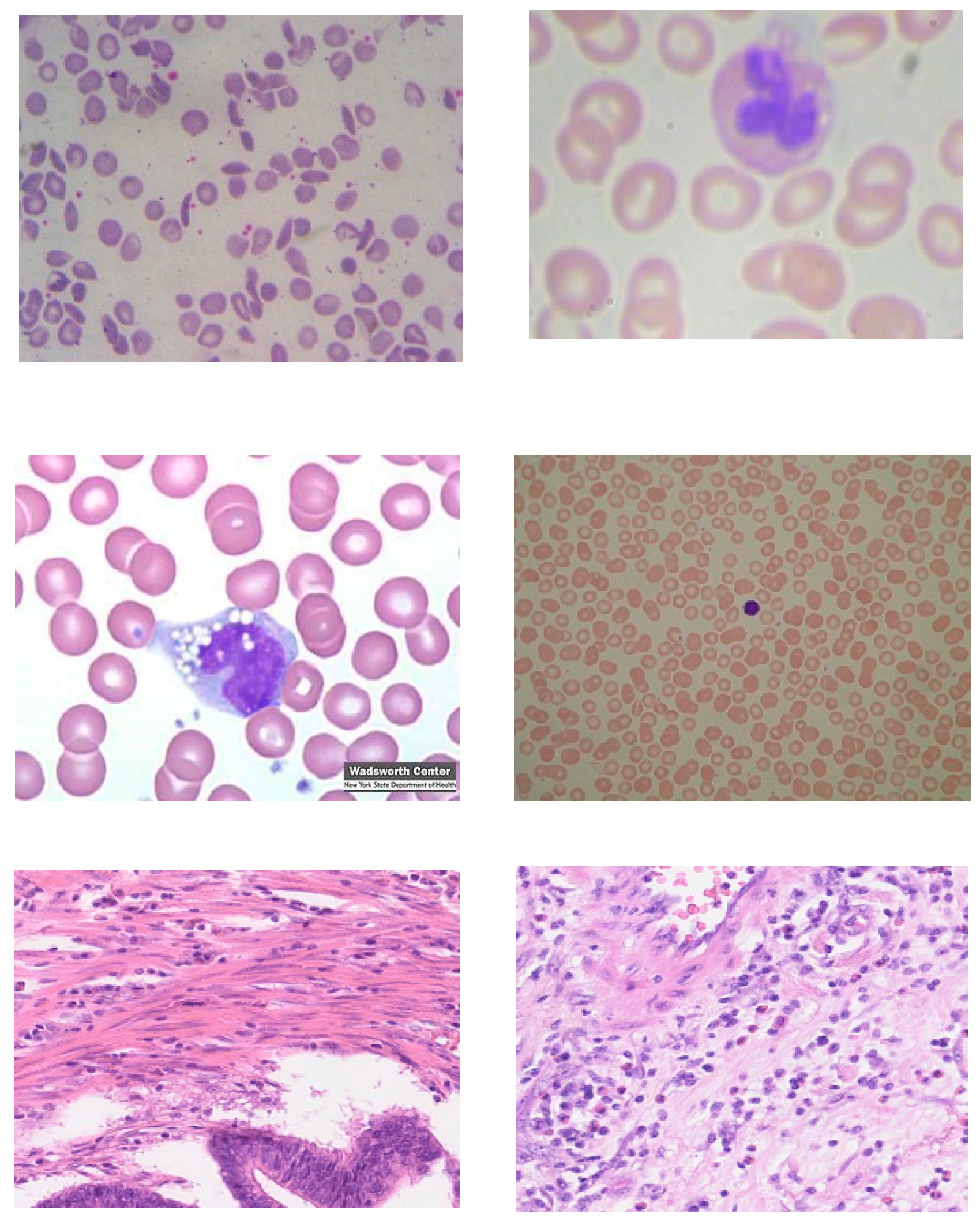
This dataset has been gathered from different sources that have microscopy images. These collected images are close to the domain of interest. The first source is the erythrocytesIDB dataset, which has images of peripheral blood smears samples taken from patients with Sickle Cell Disease in the Special Hematology Department of the General Hospital from Santiago de Cuba [43]. The dataset has 196 full-field images with a size of 3264 × 2448 pixels. This dataset is utilized to classify three types of red blood cells which are circular, elongated and other. Each image was divided into 512 × 512 samples, and the total samples produced from the dataset were 4704 samples. The second source is a white blood dataset that has 367 images of white blood cells, and other blood components [44]. This dataset is utilized to classify four types of white blood cells (Neutrophils, Eosinophils, Lymphocytes and Monocytes). Each image has a size of 640 × 480 pixels. All images have been resized to 512 × 512. The third source has 150 blood images with a size of 400 × 298 from Wadsworth center [45]. The fourth source is called the ALL-IDB2 dataset, which consists of 260 images of lymphocytes utilized for the diagnosis of acute lymphoblastic leukemia. The images are classified into two classes: normal lymphocytes and immature lymphocytes [46]. The images of this dataset have a size of 257 × 257. The fifth source is the colorectal dataset that contains 100 images of H&E-stained colorectal adenocarcinoma specimens [47]. All images of this source have a size of 500 × 500. The images of third, fourth and fifth sources have been upscaled to 512 × 512 to fit within the input size of the proposed model. Each source was considered as one class to train the proposed model. Samples from the same domain dataset are shown in Figure 3.

3.1.3. Different Domain Dataset

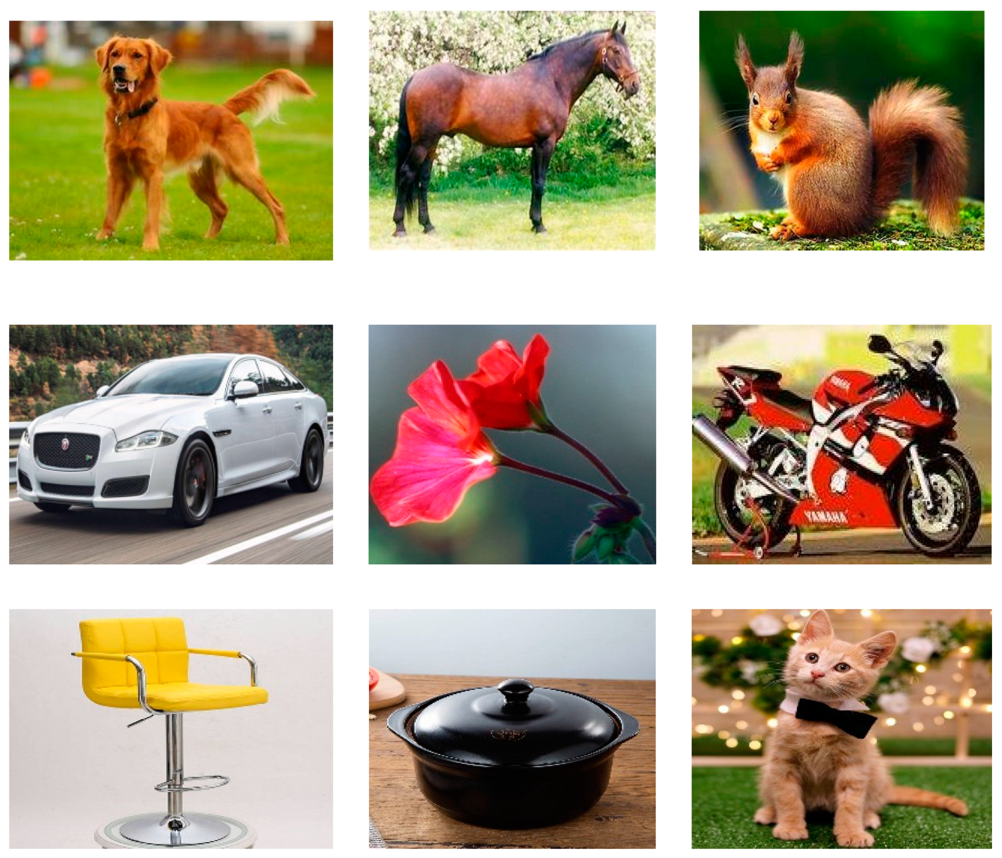
This dataset is a collection of natural images that have been gathered from different sources. The first source is a dataset that consists of six classes, which are airplane, car, flower, fruit, motorbike and person [48,49]. The total number of images is 5000 with different image sizes. The second source is a dataset that has 10 classes of animals which are a cat, dog, horse, spider, butterfly, chicken, sheep, cow, squirrel and elephant [50]. The total number of images is 26,179. The last source is a dataset with four classes, which are chair, kitchen, knife and saucepan images [51]. Each class contains 1300 images, and the total number of images is 5200. All images have been resized to 512 × 512 to fit within the input size of our proposed model. We have kept the same original labels for training our proposed model. Figure 4 shows some samples of this dataset.

3.2. Image Augmentation

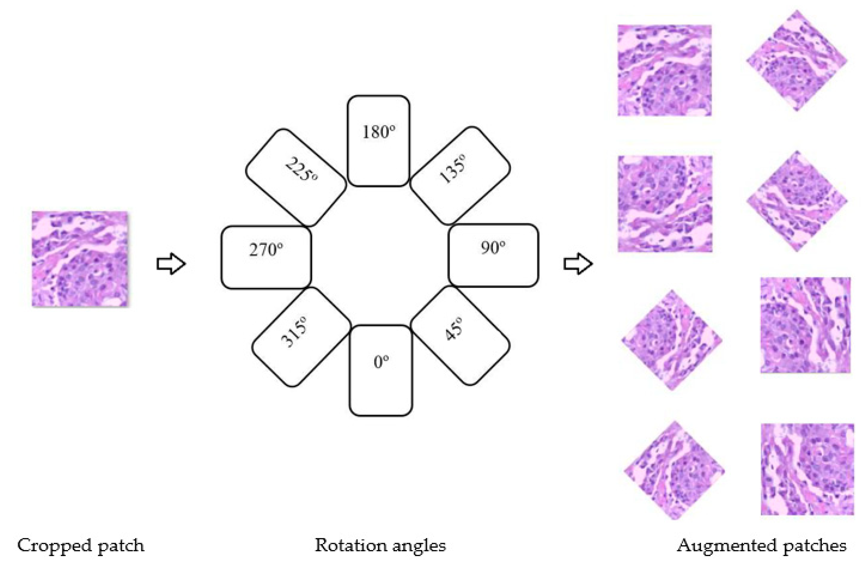
The optimization of DL performance relies on the number of training images. DL models require a big amount of training data to perform well. Lack of training images in the medical field is the main challenge for the use of DL models. The BACH 2018 challenge (ICIAR 2018 dataset) [16] is an example of a small dataset. Collecting medical images is very expensive, and requires an expert to label the images. To address this issue, we have utilized the transfer learning technique (which is explained in the next part) and image augmentation. Image augmentation is a technique that is utilized to increase the number of training images by applying a variety of image processing operations, such as rotation, flipping and lighting. This technique also aids to avoid overfitting problems [52]. In this paper, we have used rotating and flipping techniques to augment the training patches. Rotating is implemented by applying angles of 45, 90, 135, 180, 225, 270, 315 degrees, as shown in Figure 5. Horizontal and vertical flips have been applied to original images. From every single patch, nine unique patches were produced using augmentation techniques. We have chosen rotation and flipping over other techniques due to two reasons. The first reason is that clinicians can analyze histological images of breast cancer from different angles without affecting the diagnosis process. Therefore, employing image augmentation using patch rotation and flipping further enhances the dataset. The second reason is that rotation and flipping enlarge the size of the dataset without affecting the quality of the input images [39,53].

3.3. Transfer Learning

The deep CNNs are still extensively employed in current research. They offer innovative support to overcome several classification challenges. The lack of training data is a common problem in employing deep CNN models which require a large amount of data to perform well. Furthermore, collecting a large dataset is tedious, and it even now continues. Therefore, the transfer learning technique is currently employed to overcome the small dataset issue [54]. This technique is extremely effective in solving the problem of a lack of training data.
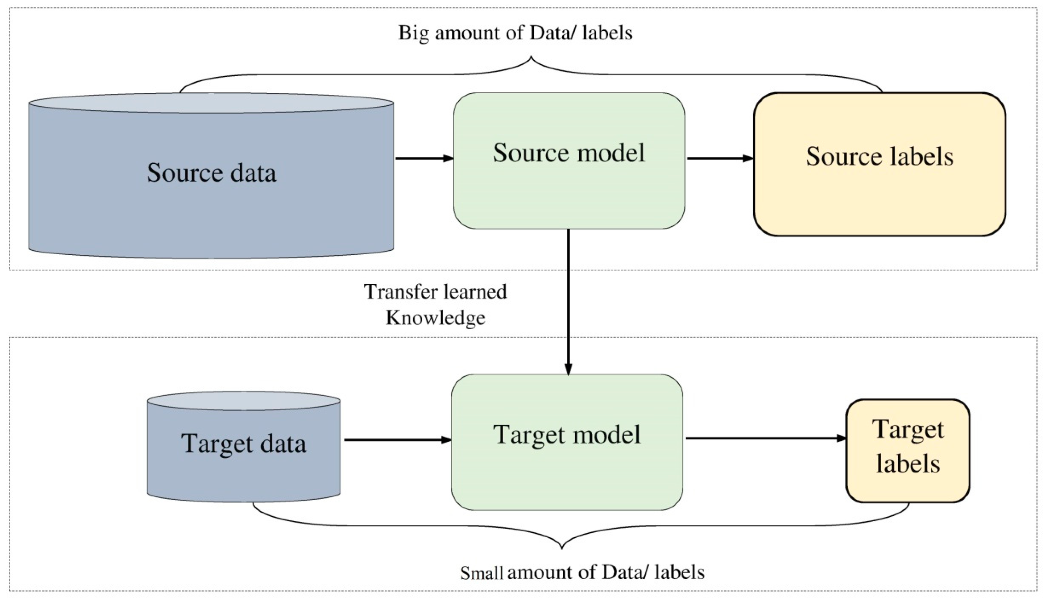
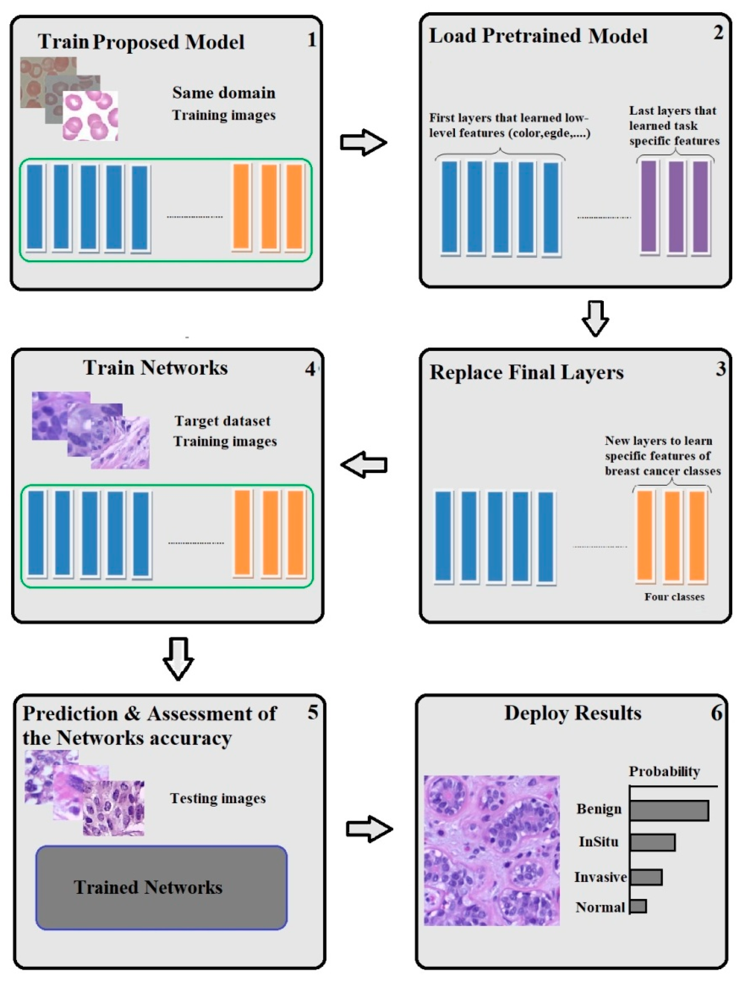
Transfer learning is a mechanism where CNNs models are trained on dataset with large amount of data, and then the models are fine-tuned to train on a small desire dataset, as shown in Figure 6.
Pre-trained state-of-the-art models, such as AlexNet, GoogleNet and ResNet trained on ImageNet dataset, have been utilized for transfer learning and showed good performance in different applications [55]. However, it was proven by the Google brain researchers that transfer learning from pre-trained state-of-the-art models does not significantly improve the performance of medical imaging tasks, due to differences in learned features domains [56].
To test this hypothesis for the breast cancer classification task, we have utilized transfer learning from two sources: transfer learning from the same domain of target task, transfer learning from the different domain of target task. The process of our transfer learning technique starts by training the proposed model on the same domain dataset. Then we fine-tune the proposed model to train over on the target dataset, which is BACH 2018 to classify four classes of hematoxylin–eosin-stained breast biopsy images, as illustrated in Figure 7. We repeat the same procedure for transfer learning from the different domain dataset.

3.4. Convolutional Neural Networks (CNNs)

CNN is one of the best Machine-Learning (ML) algorithms that is used in analyzing medical images, since it maintains the spatial relationships after filtering the input images. These relationships are extremely significant in the field of medical analysis [57,58,59]. CNN consists of multiple layers, as shown in Figure 8. These layers are:

3.4.1. Convolutional Layer

In image analysis, convolution is described as a process of two tasks. The first task includes inputting values, which represent the pixel values, at different locations in the image. The second task is a kernel (or filter), which is denoted as an array of numbers. The output is determined as the dot product between the two tasks. Then, the kernel is shifted to the following location in the image, which is denoted via the stride length. A feature map (so-called activation map) is generated from repeating the computation up to cover the whole image. This map represents where the kernel is effectively motivated, and ‘sees’ a feature like a curved edge, a dot, or a straight line. For example, when inputting a face image to a CNN, then the kernels discovered the low-level features like edges and lines, initially. The feature maps turn out to be inputs for the following layer inside the CNN structure, while the low-level features accumulated to gradually better features in the successive layers like the ear, eye, or a nose.
For performing effectively computational machine learning, convolution utilizes three essential concepts, which are invariant (equivariant) representation, weights (parameter) sharing, and sparse connections [60]. Sparse connections in CNN mean that just a few outputs of the current layer are connected to the following layer, while in some other neural networks, the whole neuron outputs of the current layer are connected to the Whole neuron inputs of the following layer. As the covered area of the kernel per stride (local reception field) is smaller, this progressively learns the significant features, and considerably decreases the calculated number of weights, which in turn, enhances the efficiency of the algorithm. CNN reduces the requirements of the memory storage by employing each kernel with its preset weight crossover various locations of the complete image, which is identified as weights sharing. In fully connected neural networks, the weights, which are much more between layers, are employed just one time and then abandoned. Weight sharing causes a rise in the quality of the invariant representation, which denotes that the translations of the input result in equivalent translations of the feature map.

3.4.2. Pooling Layer

The main function of the pooling layer is to decrease the image size (height and width only, without depth) and the calculated parameters. It follows the convolutional layer and precedes the ReLU layer. The most commonly employed pooling types are average and max pooling. Max pooling selects the highest value of the input inside a kernel and abandons the others, while average pooling takes the average of values.

3.4.3. Rectified Linear Unit (ReLU) layer

This layer is a triggering function that adjusts all negative values of the input to zero. The ReLU layer boosts and simplifies training and calculations, and helps avoiding the problem of vanishing gradient. It is mathematically defined as: f ( x ) = max ( 0 , x ) . The neuron input is represented by x. Conversely, other triggered functions involve parametric ReLU, randomized ReLU, leaky ReLU, tanh and the sigmoid functions.

3.4.4. Fully Connected Layer

The fully connected layer constitutes the last part of the CNN architecture, which means that all neurons in this layer are connected to all of the neurons in the previous layer. Based on the desired level of feature abstraction, there can be one or more, in a similar way to the pooling, ReLU and convolutional layers. This layer takes the previous layer output (pooling, ReLU, or convolutional), and calculates a probability score to classify into one of the output classes. In other words, the fully connected layer inspects the group of the highest robustly activated features that could lead to a specific class where the image fits in. For instance, on histology glass slides, the ratio of DNA to cytoplasm for cancer cells is higher than that for normal ones. The CNN could be extra tending for predicting the existence of cancer cells if the DNA features were highly distinguished from the previous layer. The CNN can be enabled to learn significant organizations from trained images using training techniques of the traditional neural network with stochastic gradient descent and backpropagation [61].

3.5. Proposed Model

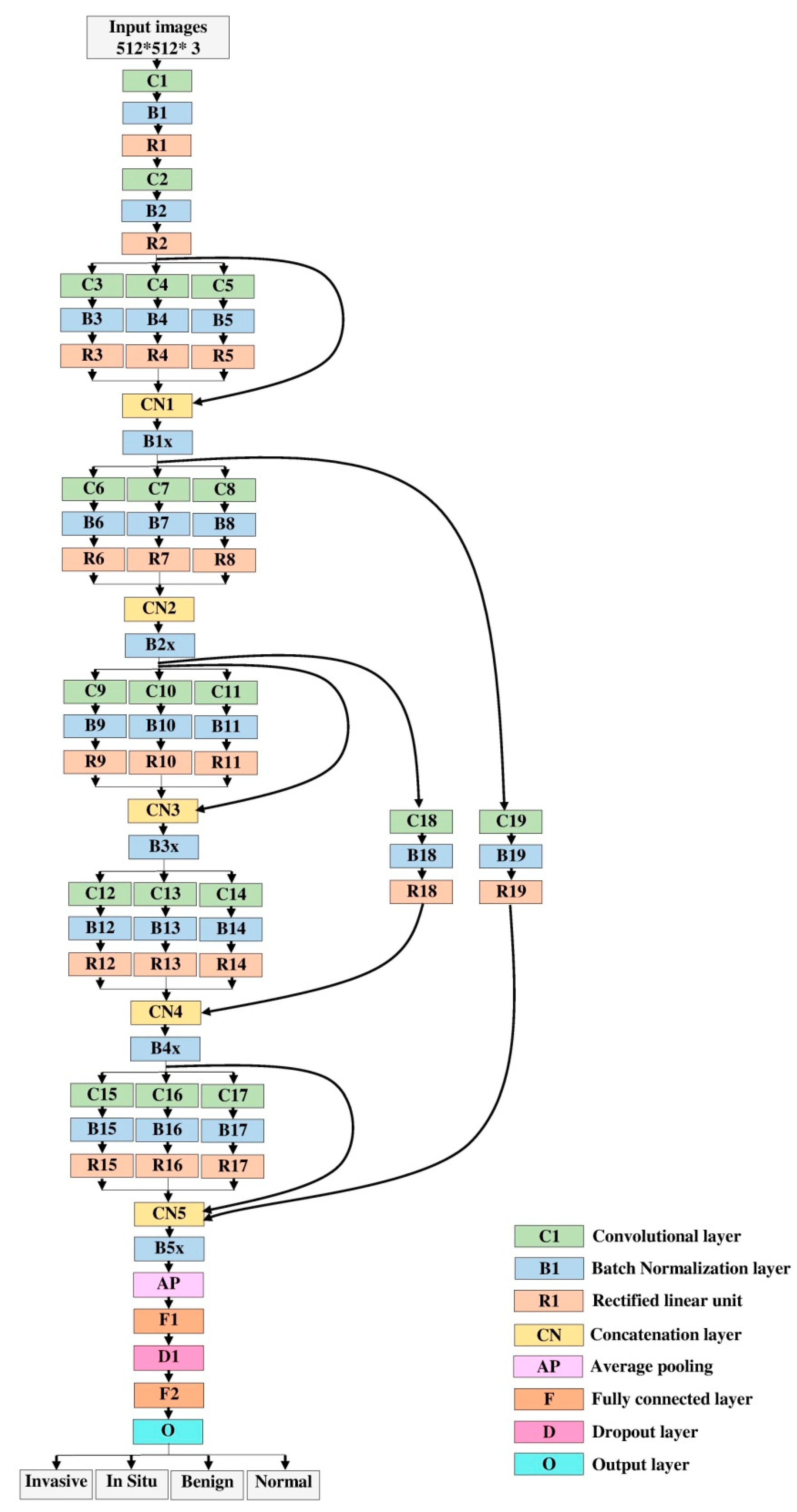
The complexity of breast cancer images makes the classification task challenging. Therefore, a deep neural network model with better feature extraction and excellent feature representation, needs to be employed for this task. Therefore, this paper proposes a hybrid deep convolutional neural network model that integrates two ideas which are a multi-branch of parallel convolutional layers and residual links to classify four types of hematoxylin–eosin-stained breast biopsy images (invasive carcinoma, in-situ carcinoma, benign tumor and normal tissue image). Our model architecture has proven to be advantageous for gradient propagation, since the error can be backpropagated via multiple routes. Furthermore, due to the integration of two ideas of the multi-branch of parallel convolutional layers and residual links, our model concatenates different levels of features at each step. Furthermore, employing residual links assists to prevent the gradients vanishing issue. These residual links are straightforwardly adding the value at the start of the block x to the last part of the block (F(x) + x). In addition, they do not pass via activation functions that squish the derivatives, causing greater total derivatives of the block. We also used short links that have some layers that use these activations, which actually is not a significant issue that affects the gradient to vanish.
We have chosen this architecture based on our study of previous state-of-the-art models, such as GoogleNet and ResNet, by knowing the benefits of employing the idea of each model. Redesigning the CNN structure in the way in which multiple branches are fused (either concatenation or summation), and the residual connection is very helpful for gradient propagation and features representations [62,63]. We have empirically tried different architectures and configurations to obtain the final architecture of the proposed model.
The proposed model architecture consists of 74 layers in total. It has 19 convolutional layers, with different filter sizes that have the function of extracting features such as edges, color and shape. The model starts with two traditional convolutional layers of 5 × 5 and 7 × 7 filter size. The purpose of employing these layers is to reduce the size of the input image. We have applied a filter size of 5 × 5 and 7 × 7 at the beginning of the model to avoid losing information that describes the nucleus-localized organization and the overall tissue architecture which is important to distinguish between classes. Employing a small filter size such as 1 × 1 will act as a bottleneck that prevents the large features which describe the architecture of the input image. Five blocks of parallel convolutions are employed after the traditional convolutional layers. Each block has three convolutional layers (1 × 1, 3 × 3, 5 × 5) that are working in parallel. We connected the five blocks with short and long connections to tackle the gradient vanishing problem. All convolutional layers in the model are followed by Batch Normalization (BN) and ReLU. After each block, there is a concatenation layer that concatenates the output of the block. This layer is followed by the BN layer. Once again, the gradient vanishing issue happens when squashing a big input space into a small space. The Rectified Linear Unit (ReLU) is a good choice among activation functions, since it is mapping x to max (zero, x), which does not produce a small derivative.
Batch normalization also aids to degrade the gradient vanishing issue. The normalization process ensures that the derivative is big enough for further actions. The main function of employing pooling layers is to reduce the dimensionality of the features received from convolution layers. Two types of pooling layers are the most used, which are max pooling and average pooling. Max pooling operates by taking the maximum values which lead to extract the most significant features, such as shapes. This type has the drawback of losing some of the less important features. Average pooling operates by taking the average of values. It guarantees that there will be a combination of significant and less significant features. Two main aspects were considered regarding the pooling layer. Firstly, we have not employed any pooling type after each convolutional layer, in order to avoid losing the features. We have utilized the average pooling layer at the end of the model to reduce the dimensionality and to maintain all features that are propagated to the end of the model. Two fully connected layers have been utilized, and between them, there is a dropout layer to prevent the overfitting issue. At the end of the model, there is a softmax function to finalize the output. Figure 9 and Table 1 detail the architecture of our proposed model.
We have trained our model in four different experiments as follows:
  • Experiment 1: Training only on the target dataset images.
  • Experiment 2: Training on target dataset images, plus augmented images of the target dataset. (these augmentation techniques are explained above)
  • Experiment 3: Training on transfer learning datasets first, then fine-tune the model and re-train it on the target dataset images.
    (a)
    We train our model from scratch on the different domain dataset first, then fine-tune our model with transferring the learning, and re-train on target dataset images
    (b)
    We train our model from scratch on the same domain dataset first, then fine-tune our model with transferring the learning and re-train on target dataset images.
  • Experiment 4: Training on transfer learning dataset plus augmented images of transfer learning dataset first, then fine-tune the model and re-train it on target dataset images plus augmented images of the target dataset. We have applied this experiment on both datasets (different and same domain datasets as explained in experiments 3 a and b).
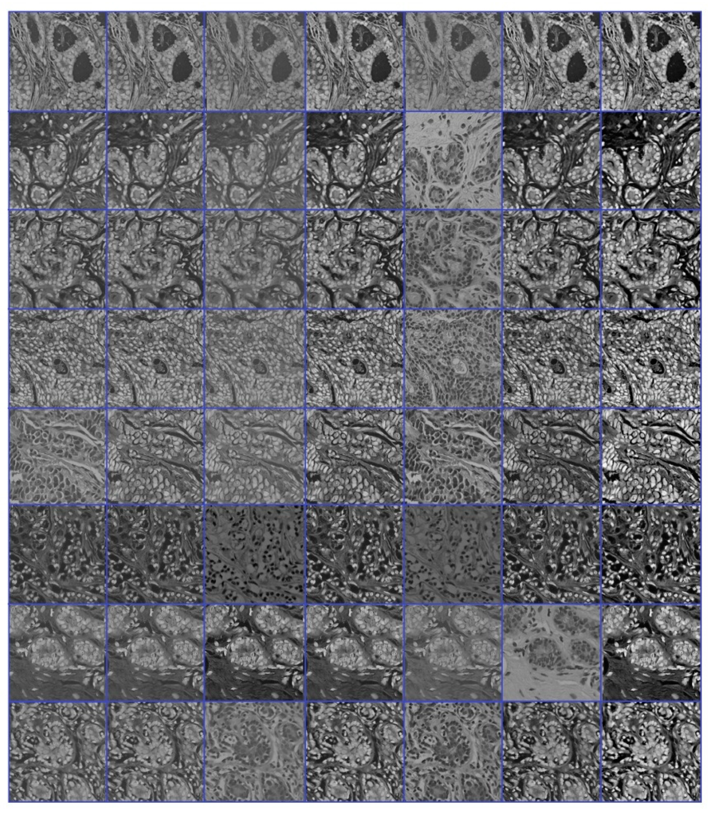
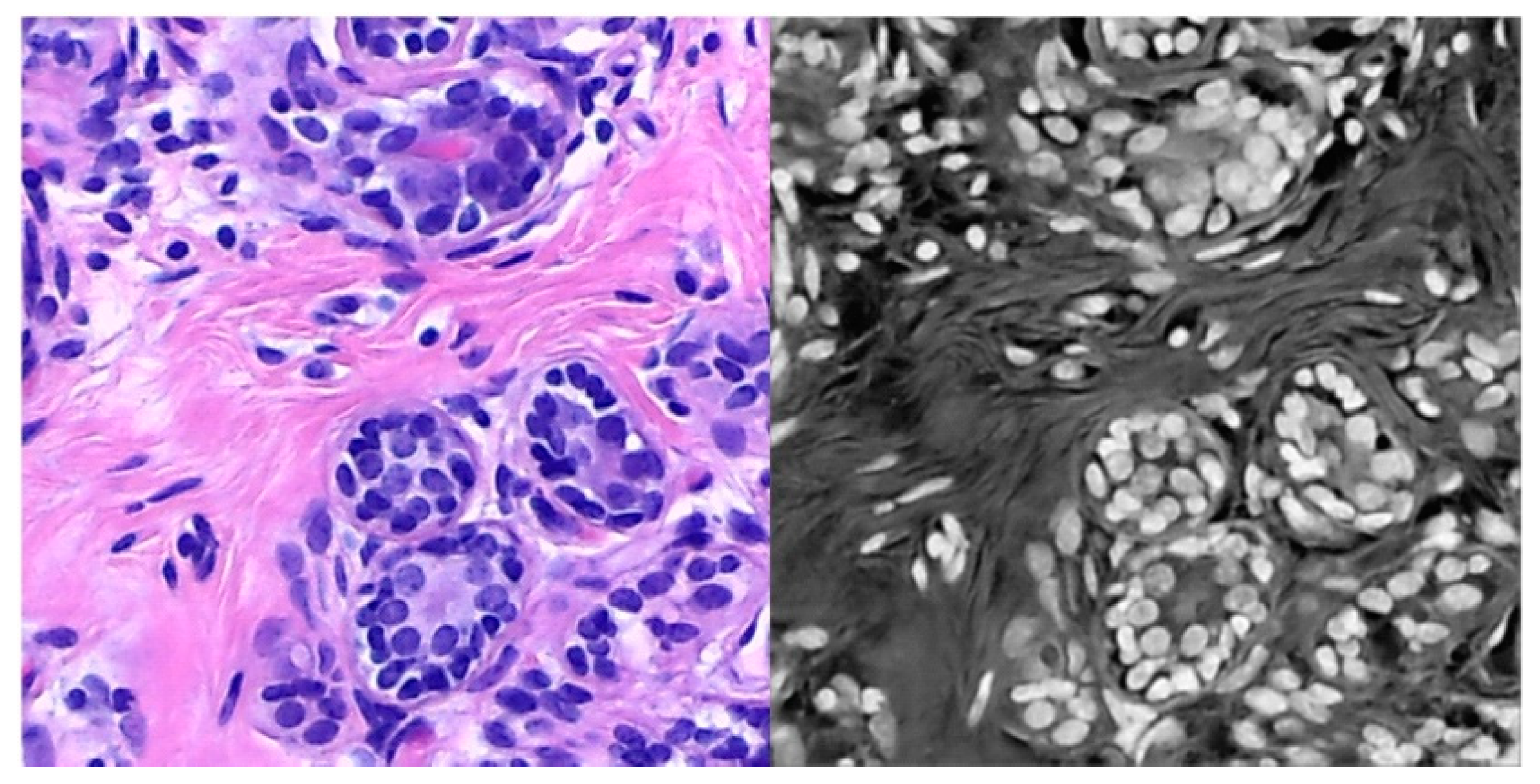
We have visualized what the first convolutional layer learned of our model trained with Experiment 4, as shown in Figure 10. Figure 11 shows learned filter from second convolutional layer of our model trained with Experiment 4. The training process was achieved utilizing Stochastic Gradient Descent with momentum set to 0.9. Mini-batch size is 64 and MaxEpochs is 120 with a learning rate that was initially set to 0.001. The training process got stabilized in epoch 100 where we stopped the training process. We have implemented our experiments on Matlab2018 as software and a processor with properties of Intel (R) Core TM i7-5829K CPU @ 3.30 GHz, the RAM was 32 GB and the GPU was 8 GB.

4. Experimental Results

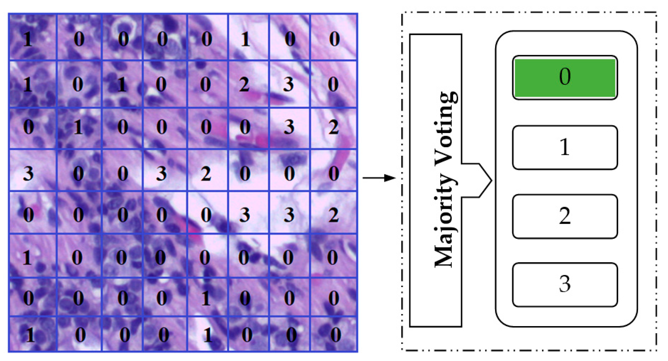
The implementation of image classification is achieved by using a patch-wise classifier to process several patches first, then voting for the most common class among patches results to gain the final image-wise classification (Figure 12).
To classify a single image, the input image is partitioned into 12 non-overlapping patches of size 512 × 512 at first. Then the probabilities of patch classes are calculated by the patch-wise trained proposed model classifier to decide the patches results. This step is called patch-wise classification. Based on the results of the patch-wise stage, the image-wise classification is accomplished by utilizing the majority voting technique applied, where the patch label, which is the most frequent, is chosen to be the image label (Figure 13). The evaluation of the overall accuracy of the process is implemented by calculating the ratio between the number of correctly classified images and the total number of images in the evaluation.
We first started by evaluating our model with four training experiments on the validation set in patch-wise and image-wise classification, as reported in Table 2. Training our model with Experiment 2 improved the results of Experiment 1 from 76.5% to 82.9% in terms of patch-wise classification, and from 80.3% to 88.1% in terms of image-wise classification. Although Experiment 2 improved the classification accuracy, it is far from our goal. The accuracy in Experiment 3 improved compared to experiments 1 and 2, using transfer learning from the same domain dataset. It achieved 87.8% and 94.1% in terms of patch-wise and image-wise, respectively. The accuracy in Experiment 4 dramatically jumped using transfer learning from the same domain dataset. It achieved the highest accuracy compared to other experiments by obtaining 90.5% and 97.4% in terms of patch-wise and image-wise, respectively.
Despite the fact that our model with experiments 3 and 4 obtained significant performance optimization using transfer learning from the same domain dataset, it showed a drop in accuracy when using transfer learning from a different domain dataset compared to same domain dataset results. It achieved 77.9% in terms of patch-wise, and 81.2% in terms of image-wise with Experiment 3. It also achieved 79.5% in terms of patch-wise, and 84.2% in terms of image-wise with Experiment 4. These results are the second-lowest results after the results of Experiment 1. We can conclude from the results of Table 2 that transfer learning from the same domain optimizes the accuracy significantly.
As cited in Table 3, we then present a comparison of our model with the latest state-of-the-art methods for the ICIAR-2018 dataset image classification, in terms of patch-wise and image-wise on the validation set. Our model with Experiment 4 using transfer learning from the same domain dataset surpassed the latest methods. It is worth mentioning that Experiment 3, using transfer learning from same domain dataset, also surpassed the latest methods.
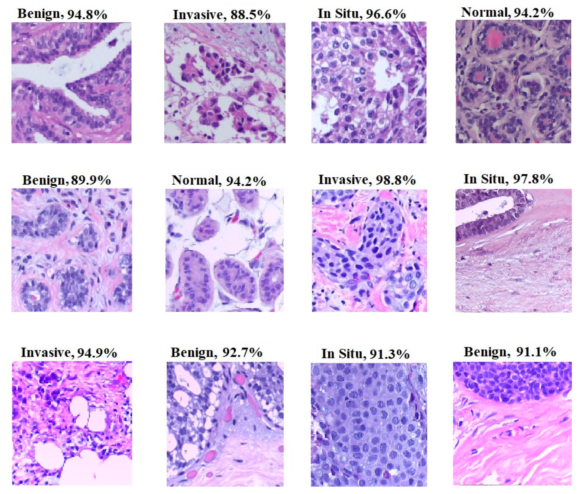
Evaluating our model on the test set of the ICIAR-2018 dataset repeats the same validation set scenario (Table 4). Our model with Experiment 4 using transfer learning from the same domain maintained the highest result by scoring 96.1%. Our model with Experiment 3 using transfer learning from the same domain achieved the second-highest result by scoring 93.8%. Experiments 3 and 4, using transfer learning from a different domain along with Experiment 1, achieved the lowest results by scoring 80.2%, 82.4 and 77.4, respectively. Experiment 2 came in the third-place after experiments 3 and 4, using transfer learning from the same domain by achieving 86.1%. With both experiments 3 and 4 using transfer learning from the same domain dataset, which involved transfer learning, proved that the transfer learning optimized the performance. The prediction of some test patches from Experiment 4 is shown in Figure 14.
Lastly, a comparison between our model and the newest methods that utilized the ICIAR-2018 dataset is presented in terms of image-wise on unseen test images of the ICIAR-2018 dataset, as listed in Table 5. Our model achieved state-of-the-art performance compared to the newest methods on the ICIAR-2018 challenge dataset. It accomplished an accuracy of 96.1% with Experiment 4.
Most of the methods listed in Table 3 and Table 5 used the pre-trained state-of-the-art models, such as AlexNet, GoogleNet, and ResNet. These models trained on the ImageNet dataset, which is a collection of natural images that learned some features that are different from the features of breast cancer images. Therefore, the performance of these methods is lower than our model that learned those features that are similar to breast cancer images. Transfer learning can slightly improve performance when the source domain is completely different from the target domain. However, using transfer learning can significantly improve the performance when the source domain is similar to the target domain, as proven by our results.

5. Conclusions and Future Work

In this paper, we presented a hybrid deep convolutional neural network to classify hematoxylin–eosin-stained breast biopsy images into four classes: invasive carcinoma, in-situ carcinoma, benign tumor and normal tissue. The model combined two concepts, which are parallel convolutions with different filter sizes and residual links. The structural design of our model has as prominent characteristics a better feature representation and the combination of features at different levels. We have presented a solution to tackle the issue of the lack of training images by using transfer learning from the same domain. Transfer learning from the same domain has changed the direction of the research that is related to breast cancer by enhancing the performance. Different experiments have been adopted to train our proposed model and to find the best training situation. The achieved results have revealed that our model obtained state-of-the-art performance in terms of breast cancer classification by accomplishing a patch-wise classification accuracy of 90.5%, and an image-wise classification accuracy of 97.4% on the validation set. It also accomplished an image-wise classification accuracy of 96.1% on the test images of ICIAR-2018. Our results outperformed the latest methods implemented for the breast cancer classification task on the ICIAR-2018 dataset. Since the idea of the same domain transfer learning improved the performance of the breast cancer classification task, we plan to use it to improve the performance of other tasks. We also plan to employ our pre-trained model to classify other tasks of microscopy images that are in the same domain.

Author Contributions

Conceptualization, L.A., M.A.F., and J.Z.; methodology, L.A., M.A.F., and J.Z.; software, L.A., J.Z.; validation, L.F., J.Z., Y.D., and O.A.-S.; data curation, L.A., M.A.F., L.F., and O.A.-S.; writing—original draft preparation, L.A., and O.A.-S.; writing—review and editing, L.A., M.A.F., O.A.-S., L.F., J.Z., Y.D.; supervision, J.Z., Y.D.; project administration, J.Z., Y.D. All authors have read and agreed to the published version of the manuscript.

Funding

This research received no external funding.

Conflicts of Interest

The authors declare that they have no conflict of interest.

References

  1. Siegel, R.L.; Miller, K.D.; Jemal, A. Cancer statistics. CA A Cancer J. Clin. 2016, 66, 7–30. [Google Scholar] [CrossRef] [Green Version]
  2. U.S. Breast Cancer Statistics. Available online: https://www.breastcancer.org/symptoms/understandfgbc/statistics (accessed on 15 November 2019).
  3. Fondón, I.; Sarmiento, A.; García, A.I.; Silvestre, M.; Eloy, C.; Polónia, A.; Aguiar, P. Automatic classification of tissue malignancy for breast carcinoma diagnosis. Comput. Biol. Med. 2018, 96, 41–51. [Google Scholar] [CrossRef] [PubMed]
  4. Breast Cancer Diagnosis; National Breast Cancer Foundation, Inc.: Dallas, TX, USA, 2015.
  5. Elston, C.W.; Ellis, I.O. Pathological prognostic factors in breast cancer. I. The value of histological grade in breast cancer: Experience from a large study with long-term follow-up. CW Elston & IO Ellis. Histopathology 1991, 19, 403–410: Author commentary. Histopathology 2002, 41, 151. [Google Scholar]
  6. Rosen, P.P. (Ed.) Rosen’s Breast Pathology, 3rd ed.; Lippincott Williams & Wilkins: Philadelphia, PA, USA, 2008. [Google Scholar]
  7. Gurcan, M.N.; Boucheron, L.; Can, A.; Madabhushi, A.; Rajpoot, N.; Yener, B. Histopathological image analysis: A review. IEEE Rev. Biomed. Eng. 2009, 2, 147. [Google Scholar] [CrossRef] [PubMed] [Green Version]
  8. Elmore, J.G.; Longton, G.M.; Carney, P.A.; Geller, B.M.; Onega, T.; Tosteson, A.N.; O’Malley, F.P. Diagnostic concordance among pathologists interpreting breast biopsy specimens. J. Am. Med Assoc. 2015, 313, 1122–1132. [Google Scholar] [CrossRef] [PubMed]
  9. Tang, J.; Rangayyan, R.M.; Xu, J.; El Naqa, I.; Yang, Y. Computer-aided detection and diagnosis of breast cancer with mammography: Recent advances. IEEE Trans. Inf. Technol. Biomed. 2009, 13, 236–251. [Google Scholar] [CrossRef] [PubMed]
  10. Huang, Z.; Lin, J.; Xu, L.; Wang, H.; Bai, T.; Pang, Y.; Meen, T.-H. Fusion High-Resolution Network for Diagnosing ChestX-ray Images. Electronics 2020, 9, 190. [Google Scholar] [CrossRef] [Green Version]
  11. Nurmaini, S.; Darmawahyuni, A.; Sakti Mukti, A.N.; Rachmatullah, M.N.; Firdaus, F.; Tutuko, B. Deep Learning-Based Stacked Denoising and Autoencoder for ECG Heartbeat Classification. Electronics 2020, 9, 135. [Google Scholar] [CrossRef] [Green Version]
  12. Yang, Z.; Leng, L.; Kim, B.-G. StoolNet for Color Classification of Stool Medical Images. Electronics 2019, 8, 1464. [Google Scholar] [CrossRef] [Green Version]
  13. Alzubaidi, L.; Fadhel, M.A.; Al-Shamma, O.; Zhang, J.; Duan, Y. Deep Learning Models for Classification of Red Blood Cells in Microscopy Images to Aid in Sickle Cell Anemia Diagnosis. Electronics 2020, 9, 427. [Google Scholar] [CrossRef] [Green Version]
  14. Abdel-Zaher, A.M.; Eldeib, A.M. Breast cancer classification using deep belief networks. Expert Syst. Appl. 2016, 46, 139–144. [Google Scholar] [CrossRef]
  15. Al-Zubaidi, L. Deep Learning Based Nuclei Detection for Quantitative Histopathology Image Analysis. Ph.D. Thesis, University of Missouri, Columbia, MO, USA, 2016. [Google Scholar]
  16. Aresta, G.; Araújo, T.; Kwok, S.; Chennamsetty, S.S.; Safwan, M.; Alex, V.; Marami, B.; Prastawa, M.; Chan, M.; Fernandez, G.; et al. Bach: Grand challenge on breast cancer histology images. Med. Image Anal. 2019, 56, 122–139. [Google Scholar] [CrossRef] [PubMed]
  17. LeCun, Y.; Bengio, Y.; Hinton, G. Deep learning. Nature 2015, 521, 436–444. [Google Scholar] [CrossRef] [PubMed]
  18. Jordan, M.I.; Mitchell, T.M. Machine learning: Trends, perspectives, and prospects. Science 2015, 349, 255–260. [Google Scholar] [CrossRef]
  19. Russakovsky, O.; Deng, J.; Su, H.; Krause, J.; Satheesh, S.; Ma, S.; Berg, A.C. ImageNet large scale visual recognition challenge. Int. J. Comput. Vis. 2015, 115, 211–252. [Google Scholar] [CrossRef] [Green Version]
  20. Kang, S.; Park, H.; Park, J.-I. CNN-Based Ternary Classification for Image Steganalysis. Electronics 2019, 8, 1225. [Google Scholar] [CrossRef] [Green Version]
  21. Alzubaidi, L.; Fadhel, M.A.; Oleiwi, S.R.; Al-Shamma, O.; Zhang, J. DFU_QUTNet: Diabetic foot ulcer classification using novel deep convolutional neural network. Multimed. Tools Appl. 2019, 1–23. [Google Scholar] [CrossRef]
  22. Fang, B.; Lu, Y.; Zhou, Z.; Li, Z.; Yan, Y.; Yang, L.; Jiao, G.; Li, G. Classification of Genetically Identical Left and Right Irises Using a Convolutional Neural Network. Electronics 2019, 8, 1109. [Google Scholar] [CrossRef] [Green Version]
  23. Krizhevsky, A.; Sutskever, I.; Hinton, G.E. Imagenet classification with deep convolutional neural networks. In Advances in Neural Information Processing Systems 25(NIPS 2012); Curran Associates Inc.: Red Hook, NY, USA, 2012; pp. 1097–1105. [Google Scholar]
  24. Szegedy, C.; Liu, W.; Jia, Y.; Sermanet, P.; Reed, S.; Anguelov, D.; Erhan, D.; Vanhoucke, V.; Rabinovich, A. Going deeper with convolutions. In Proceedings of the IEEE Conference on Computer Vision and Pattern Recognition, Boston, MA, USA, 7–12 June 2015; pp. 1–9. [Google Scholar]
  25. He, K.; Zhang, X.; Ren, S.; Sun, J. Deep residual learning for image recognition. In Proceedings of the IEEE Conference on Computer Vision and Pattern Recognition, Las Vegas, NV, USA, 27–30 June 2016; pp. 770–778. [Google Scholar]
  26. Huang, G.; Liu, Z.; Van Der Maaten, L.; Weinberger, K.Q. Densely connected convolutional networks. In Proceedings of the IEEE Conference on Computer Vision and Pattern Recognition, Honolulu, HI, USA, 21–26 July 2017; pp. 4700–4708. [Google Scholar]
  27. Kumar, A.; Kim, J.; Lyndon, D.; Fulham, M.; Feng, D. An ensemble of fine-tuned convolutional neural networks for medical image classification. IEEE J. Biomed. Health Inform. 2016, 21, 31–40. [Google Scholar] [CrossRef] [Green Version]
  28. Nawaz, W.; Ahmed, S.; Tahir, A.; Khan, H.A. Classification of breast cancer histology images using AlexNet. In International Conference Image Analysis and Recognition; Springer: Cham, Switzerland, 2018; pp. 869–876. [Google Scholar]
  29. Mahbod, A.; Ellinger, I.; Ecker, R.; Smedby, Ö.; Wang, C. Breast cancer histological image classification using fine-tuned deep network fusion. In International Conference Image Analysis and Recognition; Springer: Cham, Switzerland, 2018; pp. 754–762. [Google Scholar]
  30. Veta, M.; Pluim, J.P.; Van Diest, P.J.; Viergever, M.A. Breast cancer histopathology image analysis: A review. IEEE Trans. Biomed. Eng. 2014, 61, 1400–1411. [Google Scholar] [CrossRef]
  31. Kowal, M.; Filipczuk, P. Nuclei segmentation for computer-aided diagnosis of breast cancer. Int. J. Appl. Math. Comput. Sci. 2014, 24, 19–31. [Google Scholar] [CrossRef] [Green Version]
  32. George, Y.M.; Zayed, H.H.; Roushdy, M.I.; Elbagoury, B.M. Remote computer-aided breast cancer detection and diagnosis system based on cytological images. IEEE Syst. J. 2013, 8, 949–964. [Google Scholar] [CrossRef]
  33. Belsare, A.D.; Mushrif, M.M.; Pangarkar, M.A.; Meshram, N. Classification of breast cancer histopathology images using texture feature analysis. In Proceedings of the TENCON 2015-2015 IEEE Region 10 Conference, Macao, China, 1–4 November 2015; pp. 1–5. [Google Scholar]
  34. Brook, A.; El-Yaniv, R.; Isler, E.; Kimmel, R.; Meir, R.; Peleg, D. Breast Cancer Diagnosis from Biopsy Images Using Generic Features and SVMs (No. CS Technion Report CS-2008-07); Computer Science Department, Technion: Haifa, Israel, 2008. [Google Scholar]
  35. Zhang, B. Breast cancer diagnosis from biopsy images by serial fusion of Random Subspace ensembles. In Proceedings of the 2011 4th International Conference on Biomedical Engineering and Informatics (BMEI), Shanghai, China, 15–17 October 2011; pp. 180–186. [Google Scholar]
  36. Du, Y.-C.; Muslikhin, M.; Hsieh, T.-H.; Wang, M.-S. Stereo Vision-Based Object Recognition and Manipulation by Regions with Convolutional Neural Network. Electronics 2020, 9, 210. [Google Scholar] [CrossRef] [Green Version]
  37. Yao, H.; Zhang, X.; Zhou, X.; Liu, S. Parallel Structure Deep Neural Network Using CNN and RNN with an Attention Mechanism for Breast Cancer Histology Image Classification. Cancers 2019, 11, 1901. [Google Scholar] [CrossRef] [Green Version]
  38. Spanhol, F.A.; Oliveira, L.S.; Petitjean, C.; Heutte, L. Breast cancer histopathological image classification using convolutional neural networks. In Proceedings of the 2016 International Joint Conference on Neural Networks (IJCNN), Vancouver, BC, Canada, 24–29 July 2016; pp. 2560–2567. [Google Scholar]
  39. Cireşan, D.C.; Giusti, A.; Gambardella, L.M.; Schmidhuber, J. Mitosis detection in breast cancer histology images with deep neural networks. In Proceedings of the International Conference on Medical Image Computing and Computer-Assisted Intervention-MICCAI 2013, Nagoya, Japan, 22–26 September 2013; pp. 411–418. [Google Scholar]
  40. Cruz-Roa, A.; Basavanhally, A.; González, F.; Gilmore, H.; Feldman, M.; Ganesan, S.; Shih, N.; Tomaszewski, J.; Madabhushi, A. Automatic detection of invasive ductal carcinoma in whole slide images with convolutional neural networks. In Medical Imaging 2014: Digital Pathology; International Society for Optics and Photonics: Bellingham, WA, USA, 2014; p. 904103. [Google Scholar]
  41. Kassani, S.H.; Kassani, P.H.; Wesolowski, M.J.; Schneider, K.A.; Deters, R. Breast cancer diagnosis with transfer learning and global pooling. arXiv 2019, arXiv:1909.11839. Available online: https://arxiv.org/abs/1909.11839 (accessed on 9 December 2019).
  42. Wang, Z.; Dong, N.; Dai, W.; Rosario, S.D.; Xing, E.P. Classification of breast cancer histopathological images using convolutional neural networks with hierarchical loss and global pooling. In Proceedings of the International Conference Image Analysis and Recognition, Póvoa de Varzim, Portugal, 27–29 June 2018; pp. 745–753. [Google Scholar]
  43. Gonzalez-Hidalgo, M.; Guerrero-Pena, F.A.; Herold-Garcia, S.; Jaume-i-Capó, A.; Marrero-Fernández, P.D. Red blood cell cluster separation from digital images for use in sickle cell disease. IEEE J. Biomed. Health Inform. 2014, 19, 1514–1525. [Google Scholar] [CrossRef]
  44. Parthasarathy, D. WBC-Classification. Available online: https://github.com/dhruvp/wbc-classification/tree/master/Original_Images (accessed on 15 November 2019).
  45. Wadsworth-Center. White Blood Cell Images. Available online: https://www.wadsworth.org/ (accessed on 15 November 2019).
  46. Labati, R.D.; Piuri, V.; Scotti, F. All-IDB: The acute lymphoblastic leukemia image database for image processing. In Proceedings of the 2011 18th IEEE International Conference on Image Processing, Brussels, Belgium, 11–14 September 2011; pp. 2045–2048. [Google Scholar]
  47. Sirinukunwattana, K.; Raza, S.E.A.; Tsang, Y.W.; Snead, D.R.; Cree, I.A.; Rajpoot, N.M. Locality sensitive deep learning for detection and classification of nuclei in routine colon cancer histology images. IEEE Trans. Med. Imaging 2016, 35, 1196–1206. [Google Scholar] [CrossRef] [Green Version]
  48. Roy, P.; Ghosh, S.; Bhattacharya, S.; Pal, U. Effects of degradations on deep neural network architectures. arXiv 2018, arXiv:1807.10108. Available online: https://arxiv.org/abs/1807.10108 (accessed on 9 December 2019).
  49. Natural Images. Available online: https://www.kaggle.com/prasunroy/natural-images (accessed on 1 December 2019).
  50. Animals. Available online: https://www.kaggle.com/alessiocorrado99/animals10#translate.py (accessed on 1 December 2019).
  51. Collation. Available online: https://www.kaggle.com/mbkinaci/chair-kitchen-knife-saucepan (accessed on 1 December 2019).
  52. Shorten, C.; Khoshgoftaar, T.M. A survey on image data augmentation for deep learning. J. Big Data 2019, 6, 60. [Google Scholar] [CrossRef]
  53. Wang, J.; Perez, L. The effectiveness of data augmentation in image classification using deep learning. arXiv 2017, arXiv:1712.04621. Available online: https://arxiv.org/abs/1712.04621 (accessed on 28 November 2019).
  54. Pan, S.J.; Yang, Q. A survey on transfer learning. IEEE Trans. Knowl. Data Eng. 2009, 22, 1345–1359. [Google Scholar] [CrossRef]
  55. Baykal, E.; Dogan, H.; Ercin, M.E.; Ersoz, S.; Ekinci, M. Transfer learning with pre-trained deep convolutional neural networks for serous cell classification. Multimed. Tools Appl. 2019. [Google Scholar] [CrossRef]
  56. Raghu, M.; Zhang, C.; Kleinberg, J.; Bengio, S. Transfusion: Understanding transfer learning for medical imaging. In Proceedings of the 33rd Conference on Neural Information Processing Systems (NeurIPS 2019), Vancouver, BC, Canada, 8–14 December 2019; pp. 3342–3352. [Google Scholar]
  57. Gil-Martín, M.; Montero, J.M.; San-Segundo, R. Parkinson’s Disease Detection from Drawing Movements Using Convolutional Neural Networks. Electronics 2019, 8, 907. [Google Scholar] [CrossRef] [Green Version]
  58. Tajbakhsh, N.; Shin, J.Y.; Gurudu, S.R.; Hurst, R.T.; Kendall, C.B.; Gotway, M.B.; Liang, J. Convolutional neural networks for medical image analysis: Full training or fine tuning? IEEE Trans. Med. Imaging 2016, 35, 1299–1312. [Google Scholar] [CrossRef] [PubMed] [Green Version]
  59. Qayyum, A.; Anwar, S.M.; Awais, M.; Majid, M. Medical image retrieval using deep convolutional neural network. Neurocomputing 2017, 266, 8–20. [Google Scholar] [CrossRef] [Green Version]
  60. Goodfellow, I.; Bengio, Y.; Courville, A. Deep Learning; MIT Press: Cambridge, MA, USA, 2016. [Google Scholar]
  61. Rumelhart, D.E.; Hinton, G.E.; Williams, R.J. Learning representations by back-propagating errors. Nature 1986, 323, 533–536. [Google Scholar] [CrossRef]
  62. Lv, E.; Wang, X.; Cheng, Y.; Yu, Q. Deep ensemble network based on multi-path fusion. Artif. Intell. Rev. 2019, 52, 151–168. [Google Scholar] [CrossRef]
  63. Wang, J.; Wei, Z.; Zhang, T.; Zeng, W. Deeply-fused nets. arXiv 2016, arXiv:1605.07716. Available online: https://arxiv.org/abs/1605.07716 (accessed on 10 December 2019).
  64. Golatkar, A.; Anand, D.; Sethi, A. Classification of Breast Cancer Histology Using Deep Learning; Springer: Cham, Switzerland, 2018; pp. 837–844. [Google Scholar]
  65. Roy, K.; Banik, D.; Bhattacharjee, D.; Nasipuri, M. Patch-based system for Classification of Breast Histology images using deep learning. Comput. Med. Imaging Graph. 2019, 71, 90–103. [Google Scholar] [CrossRef]
  66. Ferreira, C.A.; Melo, T.; Sousa, P.; Meyer, M.I.; Shakibapour, E.; Costa, P.; Campilho, A. Classification of Breast Cancer Histology Images through Transfer Learning Using a Pre-Trained Inception ResNet v2; Springer: Cham, Switzerland, 2018; pp. 763–770. [Google Scholar]
  67. Awan, R.; Koohbanani, N.A.; Shaban, M.; Lisowska, A.; Rajpoot, N. Context-Aware Learning Using Transferable Features for Classification of Breast Cancer Histology Images; Springer: Cham, Switzerland, 2018; pp. 788–795. [Google Scholar]
  68. Guo, Y.; Dong, H.; Song, F.; Zhu, C.; Liu, J. Breast Cancer Histology Image Classification Based on Deep Neural Networks; Springer: Cham, Switzerland, 2018; pp. 827–836. [Google Scholar]
  69. Vang, Y.S.; Chen, Z.; Xie, X. Deep Learning Framework for Multi-Class Breast Cancer Histology Image Classification; Springer: Cham, Switzerland, 2018; pp. 914–922. [Google Scholar]
  70. Sarker, M.I.; Kim, H.; Tarasov, D.; Akhmetzanov, D. Inception Architecture and Residual Connections in Classification of Breast Cancer Histology Images. arXiv 2019, arXiv:1912.04619. Available online: https://arxiv.org/abs/1912.04619 (accessed on 22 December 2019).
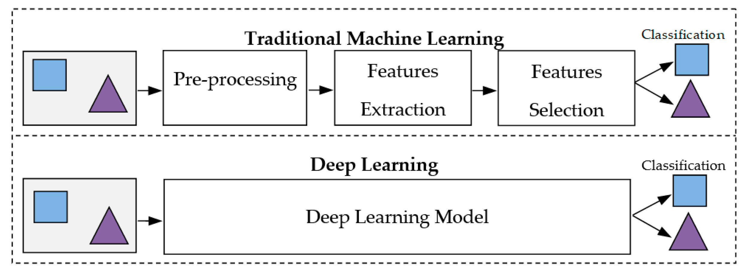
Figure 1. The difference between deep learning (DL) and traditional machine learning.
Electronics 09 00445 g001
Figure 2. Samples of the BACH 2018 dataset classes.
Electronics 09 00445 g002
Figure 3. Samples of same domain dataset.
Electronics 09 00445 g003
Figure 4. Samples of different domain dataset.
Electronics 09 00445 g004
Figure 5. Rotation process.
Electronics 09 00445 g005
Figure 6. Transfer learning technique.
Electronics 09 00445 g006
Figure 7. Transfer Learning pipeline.
Electronics 09 00445 g007
Figure 8. Convolutional Neural Network (CNN) main Layers.
Electronics 09 00445 g008
Figure 9. Our proposed model architecture.
Electronics 09 00445 g009
Figure 10. Learned filters from first convolutional layer of our model trained with Experiment 4.
Electronics 09 00445 g010
Figure 11. Learned filter from second convolutional layer of our model trained with Experiment 4, where first column is the original image; second column is the learned filter.
Electronics 09 00445 g011
Figure 12. Image-Wise classification process.
Electronics 09 00445 g012
Figure 13. Majority voting technique.
Electronics 09 00445 g013
Figure 14. Prediction of some of the test patches from Experiment 4.
Electronics 09 00445 g014
Table 1. Our model architecture, C represents Convolutional Layer, B represents Batch Normalization Layer, R represents Rectified Linear Unit layer, CN represents Concatenation Layer, AP represents Average Pooling Layer, D represents dropout layer, and F represents fully connected layer.
Name of LayerFilter Size (FS) & Stride (S)Activations
Input layer-512 × 512 × 3
C 1, B 1, R 1FS = 5 × 5, S = 1512 × 512 × 16
C 2, B 2, R 2FS = 7 × 7, S = 2256 × 256 × 16
C 3, B 3, R 3FS = 1 × 1, S = 1256 × 256 × 16
C 4, B 4, R 4FS = 3 × 3, S = 1256 × 256 × 16
C 5, B 5, R 5FS = 5 × 5, S = 1256 × 256 × 16
CN 1Four inputs256 × 256 × 64
B1xBatch Normalization
Layer
256 × 256 × 64
C 6, B 6, R 6FS = 1 × 1, S = 2128 × 128 × 32
C 7, B 7, R 7FS = 3 × 3, S = 2128 × 128 × 32
C 8, B 8, R 8FS = 5 × 5, S = 2128 × 128 × 32
CN 2Three inputs128 × 128 × 96
B2xBatch Normalization
Layer
128 × 128 × 96
C 9, B 9, R 9FS = 1 × 1, S = 1128 × 128 × 32
C 10, B 10, R 10FS = 3 × 3, S = 1128 × 128 × 32
C 11, B 11, R 11FS = 5 × 5, S = 1128 × 128 × 32
CN 3Four inputs128 × 128 × 192
B3xBatch Normalization
Layer
128 × 128 × 192
C 12, B 12, R 12FS = 1 × 1, S = 264 × 64 × 64
C 13, B 13, R 13FS = 3 × 3, S = 264 × 64 × 64
C 14, B 14, R 14FS = 5 × 5, S = 264 × 64 × 64
CN4Four inputs64 × 64 × 208
B4xBatch Normalization
Layer
64 × 64 × 208
C 15, B 15, R 15FS = 1 × 1, S = 164 × 64 × 128
C 16, B 16, R 16FS = 3 × 3, S = 164 × 64 × 128
C 17, B 17, R 17FS = 5 × 5, S = 164 × 64 × 128
CN 5Five inputs64 × 64 × 608
B5xBatch Normalization
Layer
64 × 64 × 608
C 18, B 18, R 18FS = 3 × 3, S = 264 × 64 × 16
C 19, B 19, R 19FS = 5 × 5, S = 464 × 64 × 16
APSize = 7 × 7, S = 415 × 15 × 608
F1400 FC1 × 1 × 400
D1learning rate: 0.51 × 1 × 400
F24 FC1 × 1 × 4
O (Softmax function)Invasive, In situ, Benign, Normal1 × 1 × 4
Table 2. Results of our model with training experiments on the validation set of the ICIAR-2018 dataset.
ExperimentPatch-Wise (%)Image-Wise (%)
Experiment 176.580.3
Experiment 282.988.1
Experiment 3(a) Different domain dataset77.981.2
(b) Same domain dataset87.894.1
Experiment 4(a) Different domain dataset79.584.2
(b) Same domain dataset90.597.4
Table 3. Comparative results of our model on the validation set with the latest methods on the ICIAR-2018 challenge dataset.
MethodPatch-Wise (%)Image-Wise (%)
Nawaz, W., et al. [28]75.73-
Golatkar, A., et al. [64]7985
Mahbod A., et al. [29]-88.5
Roy, K., et al. [65]77.490
Wang, Z., et al. [42]8792
Ferreira, C. A., et al. [66]-93
Our model with Experiment 4 (same domain transfer Learning)90.597.4
Table 4. Results of our model with the training experiments on the test set of the ICIAR-2018 dataset in image-wise terms.
ExperimentImage-Wise (%)
Experiment 177.4
Experiment 286.1
Experiment 3(a) Different domain dataset 80.2
(b) Same domain dataset93.8
Experiment 4(a) Different domain dataset82.4
(b) Same domain dataset 96.1
Table 5. Comparative image-wise accuracy results of our model with the latest methods on the ICIAR-2018 challenge dataset (Test Set).
MethodImage-Wise (%)
Nawaz W., et al. [28]81.25
Awan R, et al. [67]83.33
Guo Y., et al. [68]87.5
Vang Y.S., et al. [69]87.5
Sarker M., I et al. [70]89
Ferreira C.A., et al. [66]90
Kassani S. H., et al. [41]92.5
Wang, Z., et al. [42]93
Our model with Experiment 4 (same domain-transfer Learning)96.1