Article

Sequence-To-Sequence Neural Networks Inference on Embedded Processors Using Dynamic Beam Search

by
Daniele Jahier Pagliari
*,
Francesco Daghero
and
Massimo Poncino
DAUIN, Politecnico di Torino, Corso Duca degli Abruzzi 24, 10129 Turin, Italy
*
Author to whom correspondence should be addressed.
Electronics 2020, 9(2), 337; https://doi.org/10.3390/electronics9020337
Submission received: 17 January 2020 / Revised: 6 February 2020 / Accepted: 12 February 2020 / Published: 15 February 2020
(This article belongs to the Special Issue Advanced Embedded HW/SW Development)

Abstract

:
Sequence-to-sequence deep neural networks have become the state of the art for a variety of machine learning applications, ranging from neural machine translation (NMT) to speech recognition. Many mobile and Internet of Things (IoT) applications would benefit from the ability of performing sequence-to-sequence inference directly in embedded devices, thereby reducing the amount of raw data transmitted to the cloud, and obtaining benefits in terms of response latency, energy consumption and security. However, due to the high computational complexity of these models, specific optimization techniques are needed to achieve acceptable performance and energy consumption on single-core embedded processors. In this paper, we present a new optimization technique called dynamic beam search, in which the inference complexity is tuned to the difficulty of the processed input sequence at runtime. Results based on measurements on a real embedded device, and on three state-of-the-art deep learning models, show that our method is able to reduce the inference time and energy by up to 25% without loss of accuracy.

1. Introduction

In recent years, deep neural networks (NN) are increasingly gaining popularity due to their outstanding results in various tasks, such as object detection, speech recognition and image classification [1]. In particular, sequence-to-sequence networks, such as recurrent neural networks (RNNs) and the more recent transformers [2] are now considered state-of-the-art for applications involving data sequences (translation, summarization, question answering, etc.). The success of deep learning is mainly due to the increasing availability of large datasets and high performance hardware (mostly GPUs on cloud servers) to speed-up training [3,4,5].
Indeed, despite bringing an outstanding leap in accuracy, deep NNs are very computationally complex and memory-intensive. This is true not only for training, but also for the actual classification/regression (inference) phase. While for most applications training is a one-time task, and can therefore be performed in the cloud, there is a growing demand for executing NN inference on embedded systems (so-called “edge” nodes), in order to enhance the features of many Internet of Things (IoT) applications [3]. In fact, edge inference could yield benefits in terms of data privacy, response latency and energy efficiency, as it would eliminate the need of transmitting high volumes of raw data to the cloud [4,5,6,7,8,9,10,11,12,13,14,15,16,17,18,19].
However, edge devices are often equipped with low cost embedded processors and limited amounts of memory. Even more importantly, they are tightly constrained from the point of view of energy consumption, as they are expected to operate for years using the limited energy capacity of a small form-factor battery.
Various approaches have been proposed in order to reduce the complexity of deep NN inference, and consequently, its execution time and energy consumption, in order to enable its execution on edge devices. One of the most popular approaches is to design custom hardware accelerators to implement the most critical operations involved in the inference phase, which are typically multiplications of large matrices and vectors, in a fast and efficient way. Most accelerators have been designed for convolutional neural networks (CNNs), due to their outstanding results in computer vision applications [3,6,7,12,16], but more recently, hardware acceleration of sequence-to-sequence models, such as RNNs and transformers, has also been investigated extensively [10,15,17,18,19].
While these solutions are extremely effective, the addition of a dedicated hardware accelerator to an IoT device is not always feasible due to the tight cost budgets associated with this type of system. Therefore, other researchers have investigated algorithmic solutions that can improve NN inference efficiency when it is executed on general purpose embedded CPUs as well. Seminal approaches of this type include optimizations of the data representation format (i.e., quantization) aimed at reducing computational complexity and memory occupation [13,20,21] or simplifications of the network architecture [3,14,22].
However, those initial efforts are static in nature, meaning that optimizations are performed at design time and are consequently independent from the specific input datum that the network is processing. More recently, some researchers have shown that dynamic (input-dependent) optimizations, applied at runtime, can lead to superior results [5,8,9,11,23,24,25,26,27]. The rationale of dynamic solutions is that not all inputs are equally hard to process for a NN. As an example, sentences in a translation task can be easy or hard to translate depending on the existence of multiple similar interpretations [9].
Different types of dynamic inference optimizations have been proposed in literature. Some researchers have developed “big/little” systems in which two NNs of different sizes and complexities are used depending on the input complexity [5,8,11,28]. Conditional [24] and hierarchical/staged [25,26,27] inference are other effective forms of dynamic optimization. However, all these works focus on CNNs, which process fixed size inputs.
In this work, which extends [9], we apply dynamic inference optimizations to sequence-to-sequence models. Contrarily to big/little solutions, we use a single network at all times and do not rely on custom training procedures nor quantization, although all these optimizations are orthogonal to our approach. Conversely, we use a parameter of the inference algorithm, called beam width (BW), which controls the number of invocations of the network for a given input, and hence the inference time and energy consumption. Although dynamic BW optimizations have been considered in the past [29], our work is the first, to the best of our knowledge, to use this parameter for energy efficiency.
With respect to [9], the following are the main contributions of this work:
  • We propose a new policy for setting the BW at runtime depending on the input, based on Shannon’s Entropy, and compare it to the previously proposed solution based on the standard deviation of the top-k scores.
  • We test the proposed solution on three state-of-the-art sequence-to-sequence networks, with different internal architectures and targeting different applications (translation and summarization).
  • We measure the actual inference time and energy consumption obtained with our approach on a real ARM-based embedded device.
Our results show that, thanks to the proposed dynamic BW optimization, we are able to enrich the Pareto frontier [30] in the energy vs. inference quality plane, generating many previously unavailable options for designers to select at runtime. Moreover, in some instances, we are able to reduce the inference time and energy by up to 25% with no penalty in terms of output quality.

2. Background and Related Works

2.1. Encoder-Decoder Sequence-To-Sequence Neural Networks

Deep neural networks are now considered state-of-the-art for a variety of applications, ranging from computer vision to speech recognition and translation, and to radio-frequency signal processing [31,32,33,34,35,36,37]. Sequence-to-sequence neural networks process a variable length sequence of input data (a text sentence, a time series, radio signals, etc.) and produce in output another data sequence, in general of a different length (e.g., a translation of the input sentence) [31]. Most sequence-to-sequence NNs are based on the encoder-decoder (Enc/Dec) architecture schematized in Figure 1.
Internally, an Enc/Dec network actually includes two separate NNs, called the encoder and the decoder respectively (green blocks). The architecture of these two networks may vary; the standard approach is to implement both encoder and decoder as recurrent neural networks (RNNs), either with the “vanilla” architecture or with one of its variants, such as the gated recurrent unit (GRU) or the long-short term memory (LSTM). However, encoder-decoder architectures are not limited to RNNs, and can also be realized with temporal convolutional networks (TCNs) [38] or with transformer NNs [2], which have now become state-of-the-art for translation tasks.
To illustrate the high-level functionality of an Enc/Dec network during the inference phase, we will use as an example the translation of English text to German.
To perform a translation, first the encoder network processes the elements of the input sequence X = x < 1 > , , x < N > (i.e., the words of a sentence in English) and produces a representation of said sequence in a high-dimensional space. This representation is then fed to the decoder, which is in charge of producing the elements of the output sequence Y = y < 1 > , , y < M > (i.e., the words of a sentence in German). More specifically, the decoder works in “steps.” In the generic i-th step, it takes as input the encoder’s output and the elements of the output sequence translated until that point (i.e., y < 1 > , , y < i 1 > ). It uses these inputs to predict a probability distribution p < i > over all possible words of the German dictionary. The k-th element of this distribution ( p k < i > ) represents the likelihood of a “partial translation” that starts with y < 1 > , , y < i 1 > and that has y < i > equal to the k-th word of the dictionary.
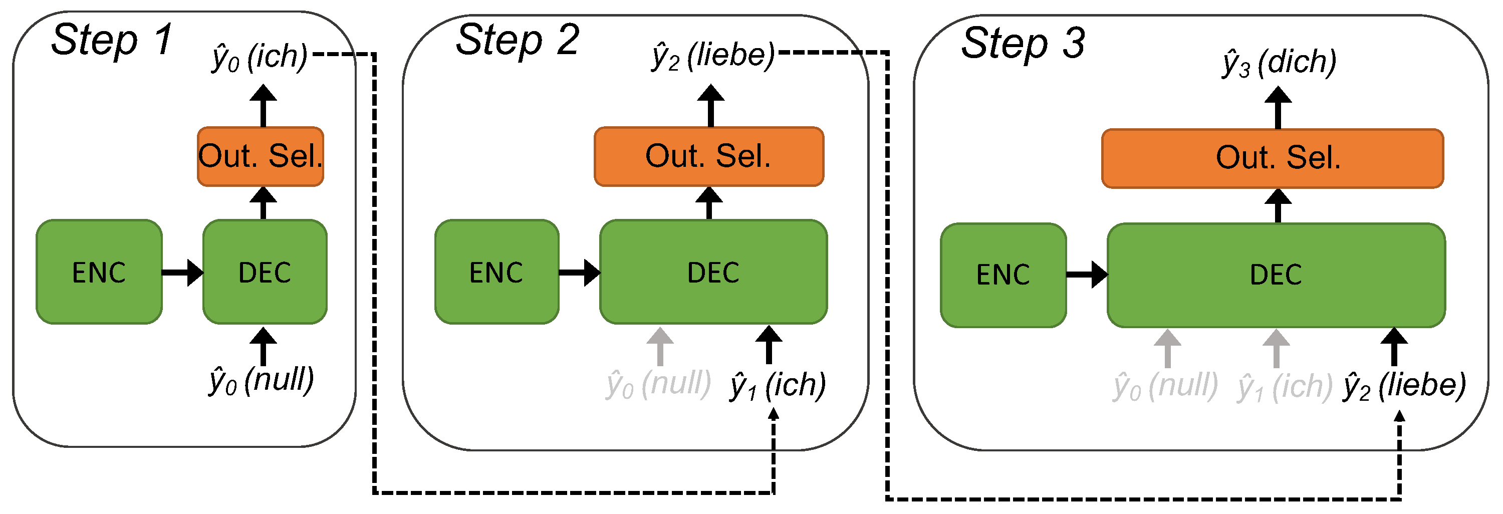
The simplest way to use the decoder during inference is shown in Figure 2. Initially, the decoder uses the encoder’s output and a “null” input to generate a probability distribution for the starting word of the output sentence. The word with the highest probability (ich in the example) is selected as the first predicted word and fed-back to the decoder, which combines it with its previous inputs to predict the second word of the sentence (liebe). This process is repeated until the decoder predicts a special end Of sentence (EOS) word.
The scheme described in Figure 2 is known as greedy search. In this approach, the output selection block (orange square in Figure 1 and Figure 2) takes into consideration only one word in each decoding step; i.e., the one corresponding to the most likely partial translation up to that point, or a r g m a x k ( p k < i > ) in mathematical terms.
However, this partial sentence does not always correspond to the beginning of the most likely translation overall. Therefore, greedily considering just one word per step may lead to discarding good translations and worsen the quality of results. For these reasons, greedy search is rarely used in practice.
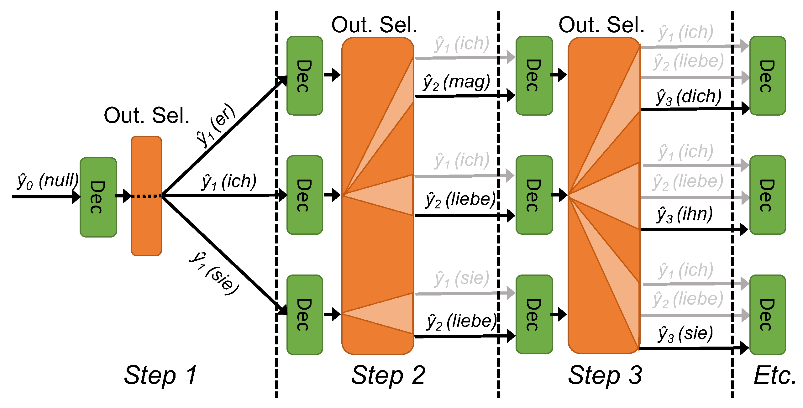
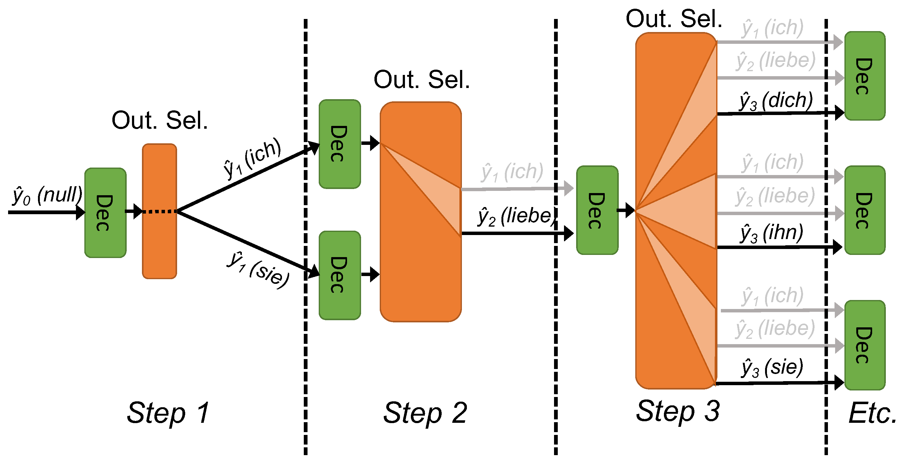
What is actually used is an algorithm called beam search, which is schematized in Figure 3 (the encoder is not drawn to avoid over-complicating the figure). With beam search, the output selection block does not sample a single word from the output dictionary. Rather, the B W most likely partial translations are kept at every step, where B W is a parameter of the algorithm called beam width. The example shown in Figure 3 corresponds to the case of B W = 3 . As is clear from the figure, in each step the decoder is invoked three times, one for each partial sentence. This generates three probability distributions, which are then considered together in the output selection phase, to identify the new three most likely partial sentences to use as input for the following step. As schematized by the light-orange “beams” in Figure 3, these may come either from different invocations of the decoder or all from the same. The three selected partial sentences are then expanded in the following step, and the whole procedure is repeated until all branches predict an EOS. In other words, beam search corresponds to expanding a tree of possible translations, where the degree at each level of the three is maintained always equal to B W .
Clearly, the one above is a very high-level description, and the details of the operation of the two NNs vary depending on their implementation. The reader can refer to [31] for more details.

2.2. Related Works

2.2.1. Custom Hardware Designs

One of the most popular approaches to obtain more energy efficient inference for neural networks is through custom hardware accelerators, targeting field-programmable gate arrays (FPGAs) [15,19,39] or application-specific integrated circuit (ASICs) [3,6,28,40]. These are custom-built architectures that optimize the most energy-intensive operations involved in the inference process (typically multiply-and-accumulate loops). The majority of custom accelerator designs have been proposed for convolutional neural networks (CNNs), particularly for image processing, while fewer works have targeted sequence to sequence architectures [18,19,41], such as the ones considered in this work. While hardware accelerators are able to improve the energy efficiency by several orders of magnitude, they are mostly suitable for high-end applications, for which a heterogeneous systems-on-chip with dedicated hardware blocks for a specific functionality can be afforded. On the contrary, due to the very tight budget constraints, most embedded and IoT devices are equipped with general purpose microprocessing units (MPUs)/microcontroller units (MCUs), and cannot afford to include such a complex custom block.

2.2.2. Static Optimizations

An orthogonal way to obtain more energy efficient inference is through approximate computing [3,4,20,42,43,44,45]. The general idea of this paradigm is to reduce the accuracy, precision or reliability of the operations involved in the inference process, in order to increase their energy efficiency. The most common form of approximate computing used in the context of deep learning is quantization, which consists in substituting the floating point operations involved in the inference with low-precision integer operations (e.g., with 8-bit or less per operand). A large number of research works have shown that applying quantization leads to more efficient deep learning models without any significant deterioration of the network accuracy [3,4,13,20,42,46,47]. The energy benefits deriving from quantization are due to two main reasons. First, replacing floating points with low-precision integers as a format for the network parameters (weights) and intermediate data (activations) significantly reduces the memory footprint of the model (e.g., by four times when using 8-bit integers), thereby reducing the energy costs for data movement. Second, the energy costs of integer operations are typically lower than those of floating point ones in MPUs/MCUs, even when a hardware floating-point unit is available.
Binarization is the most extreme form of quantization, in which either weights or activations (or both) are constrained to assume a binary value (i.e., either 0 or 1) [6,44]. In this case, besides the aforementioned memory occupation reduction, a further advantage is that most of the inference internals reduce to a sequence of bit-wise operations. However, the accuracy of binary neural networks is currently acceptable only for relatively simple tasks [44].
Another energy optimization technique that can be traced to approximate computing ideas is pruning [7,19,22,48], which consists of “switching off” those network connections (or entire neurons) that affect the output the least. These are typically selected with an iterative heuristic search algorithm, alternated with retraining phases. As for quantization, pruning leads to a reduction in the memory footprint of the network, whose weights can now be represented using a sparse matrix format, and in the energy consumption of internal operations, such as those related to “switched off” elements can be directly skipped.
Both quantization and pruning can be used in conjunction with custom hardware designs such as those mentioned above. Indeed, most of the aforementioned accelerators use quantization internally. Pruning is slightly less common because skipped computations break the regularity of the inference workload, complicating the control needed to fully utilize the parallel array of processing elements included in accelerators [3]. However, these approaches can also be applied in general purpose MPUs/MCUs, as many modern instruction sets support reduced precision operations, often in conjunction with single-instruction multiple-data (SIMD) parallelism [49,50].
As for hardware acceleration, quantization and pruning, they have mainly been applied to convolutional neural networks [4,7,13,20,42,48] and fully-connected feed-forward neural networks [4,20,47]. Fewer works have been proposed using these techniques on sequence-to-sequence models [19,22,46], mostly due to the fact that some of these models (recurrent neural networks and variants) include feed-back connections, which favor the propagation of errors and therefore hinder the application of approximate computing strategies.
Importantly, quantization and pruning are also orthogonal to dynamic algorithmic optimizations such as the one proposed in this work. In fact, most of those solutions, including ours, are based on reducing the number of operations performed to obtain the inference result. Therefore, they are equally effective both when applied on a floating point model and on an equivalent quantized model.

2.2.3. Dynamic Optimizations

All works mentioned above implement static optimizations, meaning that the changes applied to the network models to increase its energy efficiency are decided at design time. On the other hand, dynamic approaches have also been proposed in the literature [5,8,9,11,24,25,26,27,29] over the last few years.
In this case, changes to the models are applied during runtime, depending on the datum that is currently being processed by the network. This input-dependent approach makes sense when different data have different complexity, which is common in most real applications. As two intuitive examples, classifying a blurry image in which the subject occupies a small portion of the frame and is in an unfavorable orientation (e.g., a person seen from the back) is definitely more complex than classifying a clear image, with a well oriented subject occupying most of the frame. Similarly, translating a long, ambiguous sentence is also more complex than translating a short, clear one.
In these scenarios, a static optimization would either over-approximate complex inputs, thereby lowering the final accuracy, or under-approximate simple ones, wasting energy. In contrast, a dynamic approach allows one to use different “levels” of optimization depending on the input complexity, tailoring the model to the specific input.
In [11] a dynamic optimization based on a “big/little” architecture is proposed. This solution consists of two CNNs with different sizes, and consequently different energy consumption. For each new input, the “little” network is ran first. The output produced by this network is then used to compute a confidence score of the classification being correct. Depending on the value of this score, either the result of the “little” network is kept, or a new inference is executed on the same input using the “big” network. Under the assumption that most inputs are easy to classify, the “little” network will be the only one necessary most of the time. Therefore, the overall energy consumption will be similar to a solution that only uses the “little” network, but with an increased accuracy due to the selective application of the more accurate “big” network.
The drawback of this approach is that the memory required by this architecture is much larger than for a standard network, since two different sets of weights have to be stored, one for the “little” network and one for the ”big“ one. Furthermore, the effort required for model design and the time required to train the model are almost doubled. To overcome these limitations, in [5] “little” networks are derived from the layers of “big” networks, by deactivating a portion of each layer. While this solves the memory issue, it still requires a complex and non-standard training procedure. In [8] a similar approach is proposed where the “little” and “big” networks are replaced by two different quantizations of the same network. Finally, conditional inference [24] is a similar approach, in which only the initial layers of a network are used to classify easy inputs. When the confidence scores of these “partial” classifiers are low (i.e., for difficult inputs), the remaining layers of the network are executed.
Hierarchical (or staged) inference [25,26,27] is another form of algorithmic dynamic optimization. In this case, the overall task is split into sub-tasks of increasing complexity, each performed by a differently optimized model. For example, an automated medical diagnosis can be split first by a healthy vs. unhealthy classification, and then followed by a more precise classification of the type of disease [25]. The former is then performed using a simpler network (e.g., smaller or more aggressively quantized), while the latter is left to a larger and more resource-consuming network, which is however invoked only when the first classification result is “unhealthy.”
The great majority of dynamic optimization techniques for deep learning have been proposed for convolutional or fully-connected networks. In the context of sequence-to-sequence architectures, the only approach similar to ours is the one of [29], which however, does not target energy efficiency. To the best of our knowledge, ours is the first dynamic optimization approach at the algorithm level for energy reduction that applies to generic sequence-to-sequence models.

3. Proposed Method

3.1. Motivation

As mentioned in Section 2.1, sequence-to-sequence models often rely on the beam search algorithm to explore the space of possible output sequences during decoding. The main parameter of this approach, controlling the width of the search tree (that is, the number of partial sequences kept at each decoding step) is the beam width (BW). This value has a considerable impact both on the accuracy of the results and on the inference complexity. Setting BW to 1 corresponds to using greedy search, with low memory and computational requirements, but leading to suboptimal results. With larger values of BW, the final accuracy improves substantially, but the memory requirements and the number of computations grow as well.
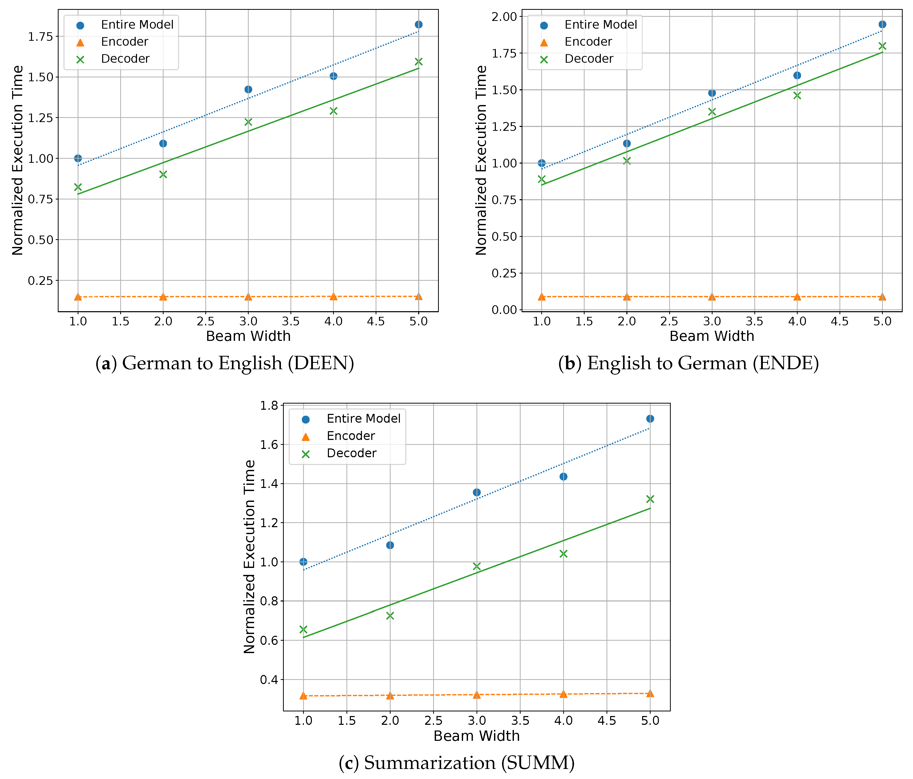
High end servers can handle large values of BW through parallelization on multi-core CPUs or GPUs. In contrast, edge IoT devices are normally equipped with an embedded CPU, often single-core, and no GPU. In the single-core scenario, it is easy to see that an increase in BW would result in a linearly proportional increase of the execution time of each decoder step, since the BW “Dec” calls in each step of Figure 3 have to be executed sequentially. This is confirmed by the plots of Figure 4, which show the dependency between the average inference time per input sequence (normalized to the case of BW = 1) and the value of BW. The three plots refer to the three models considered in our experiments and are obtained by profiling a real embedded processor (ARM Cortex-A53). Both the models and the hardware platform will be described in Section 4.
The measurements for different BWs in the graphs are linearly interpolated, to show that indeed the dependency is almost linear, although not exactly due to the optimizations performed by the inference framework (e.g., the use of SIMD instructions). Besides the overall execution time of the model, the graphs also show the individual contributions of the encoder and decoder networks. As expected, encoding time is independent from BW, whereas the increase in the overall model execution time is mostly due to the decoder. This breakdown also shows that the decoder contributes to a significant portion of the overall inference time; hence, optimizing it, as we do in this work, is relevant.
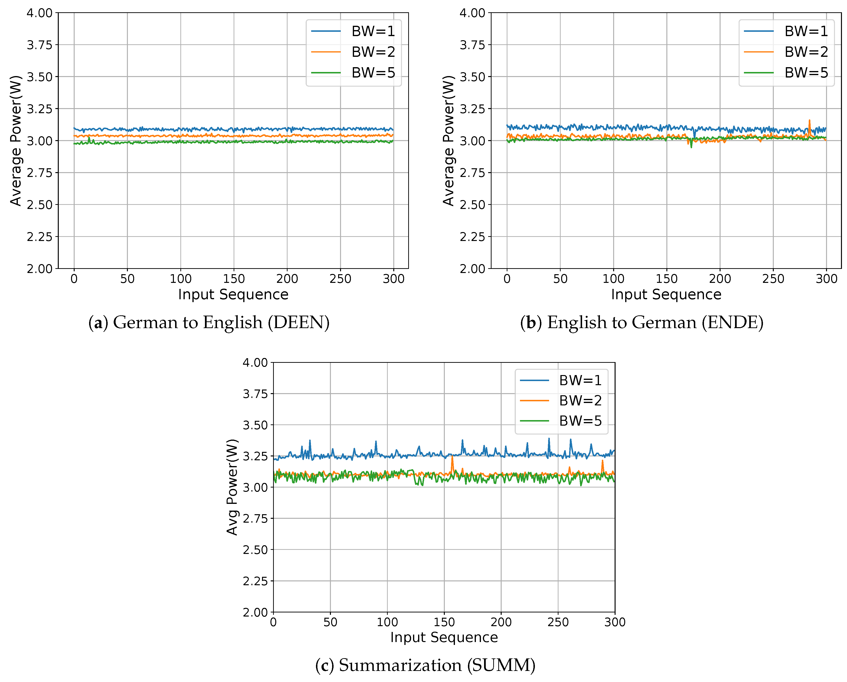
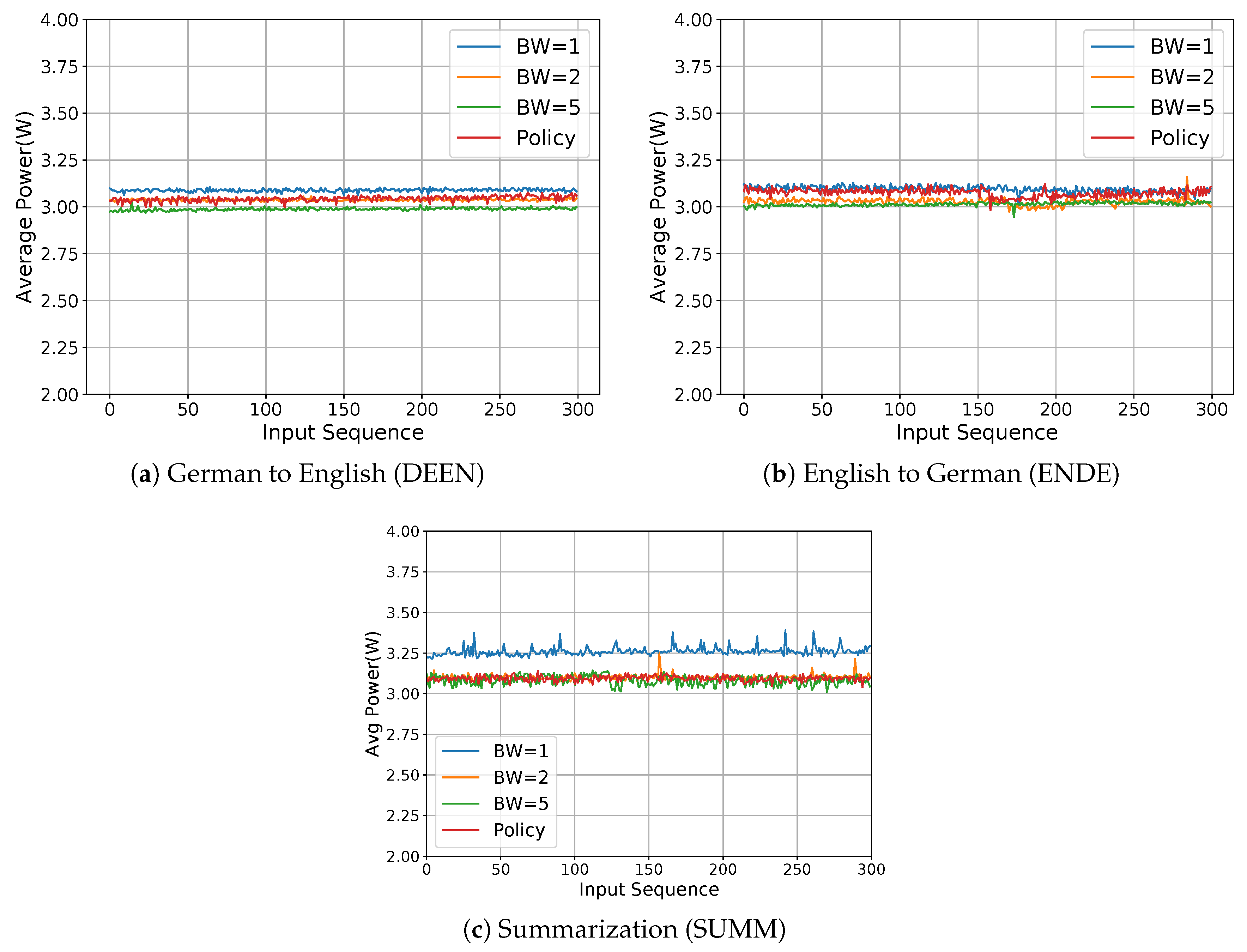
Additionally, whatever the type of model used (e.g., a LSTM rather than a Transformer) each “Dec” step involves exactly the same operations, consisting mostly of large matrix and vector multiplications. Therefore, the power consumption of a single-core CPU should remain constant throughout the inference, regardless of BW. This is confirmed by Figure 5, showing the average power per input sequence measured on the same embedded device for the three models, and for three different BW values. The plots report the total power of the embedded board, which has a baseline consumption of 1.77 W when idle. As shown, power remains approximately constant during inference and is actually slightly larger for BW = 1 (again probably due to hardware-related optimizations).
This means that, similarly to execution time, energy consumption can also be expected to grow linearly with BW. These two observations motivate our proposed technique. In fact, they show that reducing the average BW used by a sequence-to-sequence model could yield a simultaneous reduction of the execution time and of the energy consumed by an embedded device. In the following, we show how this reduction can be achieved by dynamically adapting BW to the processed input.

3.2. Dynamic Beam Search

For many deep learning tasks, data might not be all equally difficult to process, and sequence-to-sequence models are not an exception in this regard. In fact, some inputs can be easily decoded, since few partial sequences are much more likely then the others. In this case, a large value of BW would result in more computations then necessary, with a consequent waste of time and energy. Other inputs are much harder to process and require keeping more partial sequences in order to produce an acceptable quality output. In this case, a small BW would yield poor accuracy.
In this work, we propose dynamic beam search; i.e., a solution in which BW is adapted dynamically at each decoding step depending on the difficulty of the processed input.
Figure 6 shows, schematically, the decoding process performed by the network when using this technique. The differences with respect to a standard beam search are embedded in the output selection block, which determines the number of partial sequences to keep in the next decoding step based on the outputs from the current step. In the example of Figure 6, the number of decoder calls is first expanded to 2; then reduced to 1; and finally expanded again to 3.
More specifically, we propose to use the output probabilities produced by the decoder as a proxy for the number of partial sequences that should be expanded in the next step. The general intuition behind this association is that if the distribution of output probabilities is very skewed, then few partial sequences are much more probable than others; hence, BW should be decreased, and vice versa.
Clearly, the effectiveness of dynamic beam search depends on the availability of an actual mapping policy, able to map such probability distribution to the appropriate BW value for the next step. In the following section we describe two of such policies: the first one is based on Shannon’s entropy, which is a formal measure of the uncertainty of a distribution, whereas the second one is based on a heuristic estimate of such uncertainty computed using only the top-k output probabilities. The two policies are then compared experimentally in Section 4.
Importantly, besides being able to yield accurate results, mapping policies should also be fast to compute on low-end hardware. In fact, their evaluation must be executed after each decoding step. Thus, the time and energy overhead that they introduce should be minimal, to avoid overshadowing the benefits of dynamic beam search. This motivates the analysis of heuristic solutions.

3.2.1. Entropy Mapping

The first BW mapping policy considered in our work is based on computing the Shannons’ Entropy (H) on the output probabilities produced by the decoder; i.e.,
H = i N l o g e ( P i ) P i
The natural logarithm is used instead of the classical base-2, because many popular deep learning frameworks, including the one used in this work, allow sequence-to-sequence models to directly produce log-probabilities (in base e) as outputs. Consequently, using base-e avoids the base change and reduces the computational burden associated with the evaluation of (1).
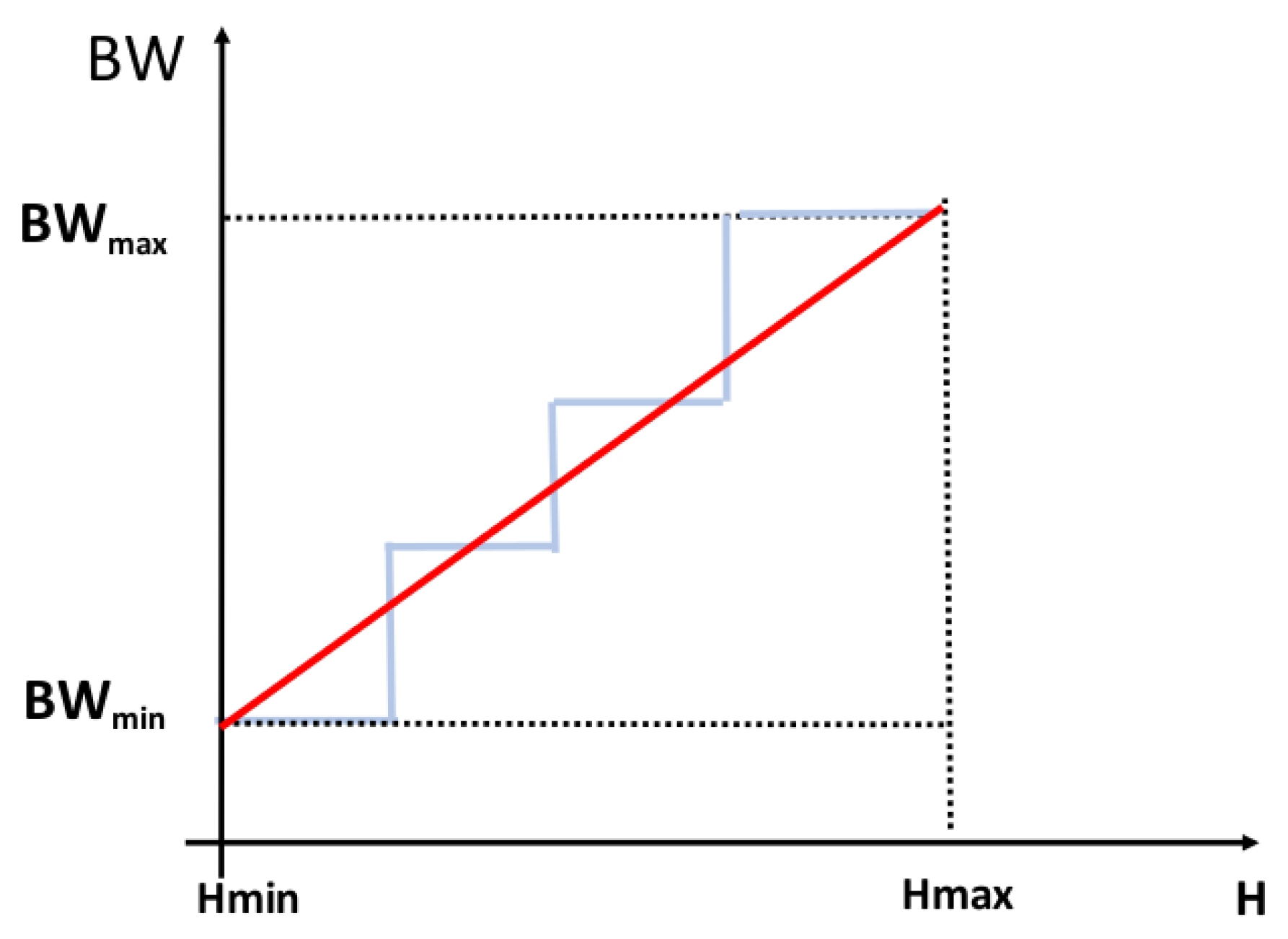
The computed entropy is then mapped to a corresponding BW using (conceptually) a line equation, as shown by the red curve of Figure 7. Smaller values of entropy correspond to a lower average uncertainty, and therefore to a higher “confidence” of the decoder in selecting the most likely partial sequences. Consequently, these values are mapped to smaller beam widths. On the contrary, larger values of H correspond to a more uncertain distribution, and are therefore mapped to a larger B W . Clearly, since B W can only assume integer values, the linear mapping is actually rounded to the nearest integer, effectively producing the relationship shown by the blue line in Figure 7.
This policy introduces four new hyper-parameters associated with the inference algorithm: the minimum and the maximum beam width accepted ( B W m i n , B W m a x ) and the parameters of the line equation (slope and intercept). These four parameters need to be tuned on the target dataset in order for the policy to be effective.
The entropy, being a measure of uncertainty, is a formally correct way to measure how “confused” the network is about the current input. While this is a desirable property, this policy uses the entire array of output probabilities in order to estimate uncertainty. Therefore, the overheads associated with its evaluation can be non negligible on a low-end device.

3.2.2. Standard Deviation Mapping

This policy, first introduced in [9], estimates the confidence of the network using only the top-k probabilities from the decoder outputs. The idea behind this approach is that only the most probable partial sequences will be selected for expansion in the next decoding step. Therefore, in order to set the optimal BW, it is sufficient to estimate how different these top probabilities are among each other. This is done computing their standard deviation, which is a simple measure of variability in a sample.
The standard deviation is then associated to a value of BW, using again, a linear mapping, as shown in Figure 8. However, this time the slope of the curve is negative, since larger values of standard deviation correspond to a bigger difference among the top-k scores, which should be associated with a smaller BW, and vice versa.
This policy is significantly faster to evaluate than the entropy mapping. However, it is clearly a heuristic, since it does not consider the entire array of output probabilities. In this case, five new hyper-parameters are associated with the inference process: B W m i n and B m a x , the slope and intercept of the curve, and the value of k; i.e., the number of top scores considered.

3.3. Implementation Details

In this section, we focus on some of the implementation details of the proposed dynamic beam search technique, and on the steps required to deploy it on an embedded device.
Importantly, dynamic beam search only modifies the inference algorithm, and not the actual sequence-to-sequence neural network. This means that, although deploying this technique on top of an existing model does require some code modifications (to support the variable BW), dynamic beam search can be applied to pretrained models without the need for retraining. This is an important feature, not only because it makes deployment faster, but also because it does not require the availability of training data, which for advanced sequence-to-sequence models is not always easily accessible [51,52].
Another consequence of dynamic beam search not requiring modifications of the underlying neural network architecture is that this approach can be applied on top of any model. Therefore, our technique is orthogonal to (and can be combined with) NN architecture optimizations targeting efficiency, such as compression methods (quantization, pruning, etc.) [3,4,13,20,42,46,47].
Moreover, dynamic beam search is also almost fully orthogonal to the framework used to describe the model (e.g., TensorFlow or PyTorch [53,54]). The only requirement is that the framework supports a dynamic computation graph; that is, that tensors dimensions can be varied during the inference process. This is required since in practice, increasing/decreasing BW involves changing one of the dimensions of the input tensors passed to the decoder in the next step. PyTorch has always supported dynamic computation graphs, whereas TensorFlow has recently added support for them. Therefore, the proposed technique can be applied on top of either framework.
The use of dynamic graphs also influences the memory occupation of our proposed method. Since the underlying neural network is not modified when using dynamic beam search, the weights and biases memory sizes do not change. The only tensor sizes that are influenced by our techniques are those related to the decoder inputs and activations, which are replicated B W i times, where B W i is the beam width used at decoding step i. However, this is true for both fixed beam search with B W > 1 and dynamic beam search; therefore, it cannot be considered an overhead of our method. In particular, the maximal inputs and activations’ memory used by our method is equal to the one used by a fixed beam search approach with B W = B W m a x . In any case, the additional memory due to replicating inputs and activations is minimal; for example, for the summarization (SUMM) network introduced in Section 4, moving from a BW of 1 to a BW of 5 only requires 1.4% more memory.
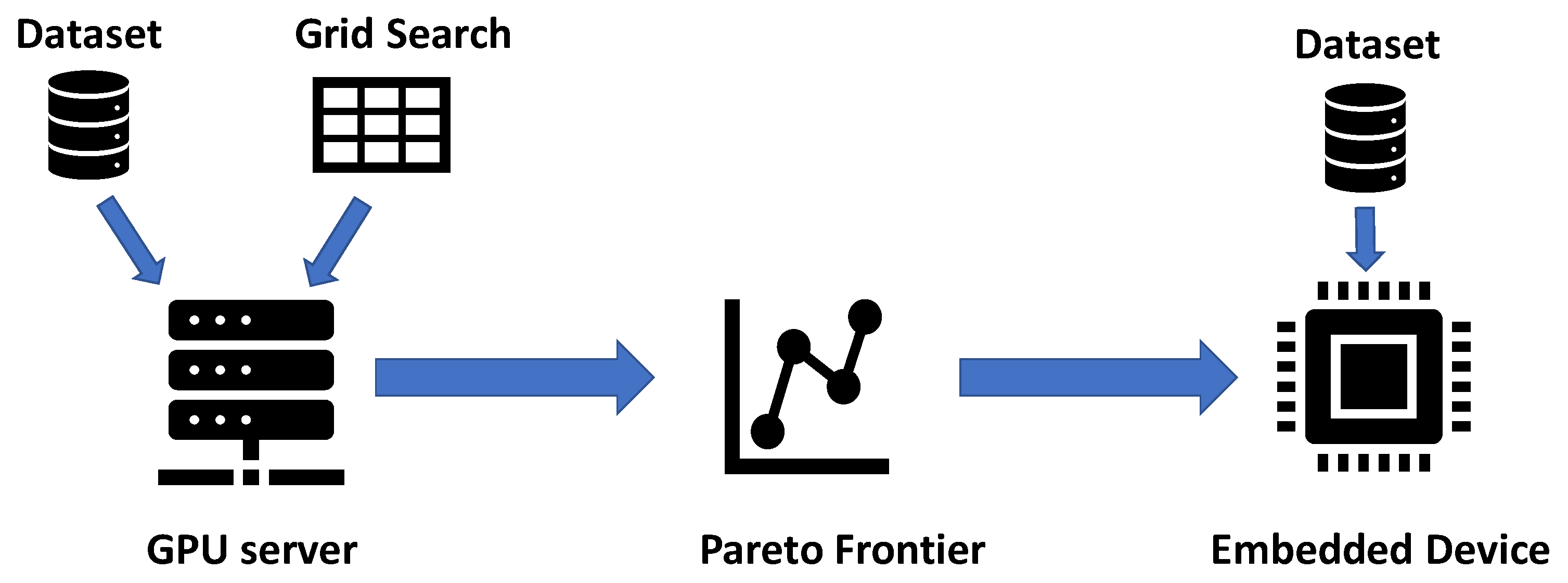
Despite not requiring training, implementing dynamic beam search still involves tuning the hyper-parameters of the two policies described in Section 3.2.1 and Section 3.2.2 for the target dataset. The typical solution to perform this kind of tuning is to run a grid-search on validation data. However, doing so directly on the embedded device would be time-expensive, given that the validation set may contain a large number of inputs and that the target device is inherently slow. Therefore, we propose to follow the procedure depicted in Figure 9.
In this approach, grid search is performed on a high-end device, such as a GPU, in order to evaluate hundreds of design points (i.e., combinations of hyper-parameters) in a reasonable time. For each point, a full inference on the entire validation set is performed using dynamic beam search, and the obtained accuracy is recorded, together with the average BW. Having completed this process, we propose to extract the Pareto frontier in the accuracy versus BW space, and only evaluate those Pareto points on the actual embedded device. In this way, the number of measurements performed on the final system, and hence the measurement time, are dramatically reduced.
The conversion between accuracy versus BW and accuracy versus time/energy Pareto frontiers follows from the analysis of Section 3.1, according to which BW is almost linearly proportional to both time and energy. Note that this certainly does not hold for the GPU used for the grid-search, which is massively parallel, and this is the reason why we store results in terms of average BW and not execution time. Under this assumption, moving from the average BW to the average execution time/energy per sentence does not alter the relationship between the different design points tested, nor, therefore, the Pareto frontier. As shown in Section 4, this method is effective at producing good settings of the considered hyper-parameters.

4. Results

4.1. Setup

The proposed methodology has been tested on three different sequence-to-sequence models, two performing a translation task and one performing summarization [55]. In particular, we selected the three recent models (>2017), each based on a different (state-of-the-art) neural network architecture; i.e., LSTM, bidirectional LSTM (BiLSTM) and a transformer.
Among the translation networks, the first one is a RNN which translates German to English (DEEN). It is composed of two BiLSTM layers with hidden size 500 (total number of parameters ≈ 50 M), and it was trained for 20 epochs on the IWSLT ’14 DE-EN dataset [32]. The second one is a transformer performing the translation from English to German (ENDE). It is composed of six layers, each with a 512-dimensional output (total number of parameters ≈ 90M), and it was trained on the WMT dataset [33]. The last network is a RNN for English summarization (SUMM). It is composed of two LSTM layers with hidden size 500 (total number of parameters ≈ 85M), and it was trained for 20 epochs on the Gigaword dataset [34].
Specifications of these models compatible with the OpenNMT framework in its PyTorch-based version are available pretrained on the official OpenNMT website [55]. This framework was used as a starting point to implement the dynamic beam search algorithm due to its ease of use and flexibility. Moreover, the fact that OpenNMT is built on top of PyTorch enables the manipulation of dynamic computation graphs at runtime, which—as mentioned in Section 3—is fundamental for the proposed optimization. The default beam width in the original networks is five for all the three models. Throughout our experiments, we always used the original trained models from OpenNMT; i.e., we did not perform any form of retraining.
The initial hyper-parameter exploration to derive the Pareto frontier in the accuracy versus beam width space was performed on a NVIDIA Titan XP GPU. Then, execution time and energy measurements were performed on an embedded device equipped with a ARM Cortex-A53 and 1 GB RAM. To emulate a real-time application, in which the response latency must be minimized, the inference batch size was set to one in all experiments on the embedded device.
Execution time measurements on the DEEN and ENDE networks have been performed on their full validation sets, while for the SUMM network we used a reduced version of the Gigaword validation set (2000 sentences randomly extracted and kept the same for all the tests) in order to have a reasonable testing time. The accuracies of the models were measured with the standard metric for the corresponding application. In particular, the quality of the translations was measured with the BiLingual Evaluation Understudy (BLEU) [56] score, and that of summarization with the Recall-Oriented Understudy for Gisting Evaluation (ROUGE) [57] score. Energy measurements were performed by attaching a digital multimeter (HP/Agilent-34401A) to a thermally stable 1mOhm shunt resistor, connected in series to the supply pin of the embedded board. Energy for all three networks was measured by letting the embedded board perform inference on 300 randomly selected inputs from the corresponding validation datasets. Since ours is the first energy-efficiency-oriented dynamic inference optimization technique for sequence-to-sequence models, we can only compare it against the state-of-the-art; i.e., a standard beam search approach with fixed BW. The fact that the three benchmarks are based on different types of models is functional for demonstrating that our approach is effective regardless of the underlying neural network architecture.

4.2. Design Space Exploration Results

As the first results, Table 1 reports the statistics of the design space exploration (DSE) process performed on the two BW mapping policies. The table reports the total number of hyper-parameters settings (total points) considered for each of the three models, and the corresponding DSE time on GPU. It also reports the number of Pareto points that have been selected for further experimentation on the actual embedded device, and the ratio between this number and the total number of points. We considered the same number of hyper-parameters combinations for each of the two policies, for fairness of comparison, and the numbers in the table refer to a single policy. Therefore, the total numbers for the entire exploration process are obtained by doubling the value in each cell. To get to the final Pareto points, we further pruned the original Pareto front, removing points that were too similar in terms of accuracy and average BW. The pruned set of points was used in all following experiments.
These results show that the DSE methodology introduced in Section 3 is indeed necessary. In fact, the total DSE time is already very significant on a high-end GPU, and it would become unacceptable (in the order of weeks/months) if the entire exploration had to be performed directly on the embedded device.

4.3. Mapping Policies Overheads

In this section, we evaluate the overheads of the two proposed BW mapping policies in terms of time and power consumption. For what concerns time, the minimum, maximum and median evaluation times for the two policies on each target model are reported in Table 2. As shown, the standard deviation mapping policy (Std. Dev.) is significantly faster than the entropy mapping for the same model. This was expected, as the former only operates on the top-k output probabilities, whereas the latter considers the entire array of probabilities. However, the time overhead of both policies is minimal. In fact, the computation of the next BW to use in dynamic beam search takes less than 1% of the average inference time (in the order of seconds for BW=1) on the SUMM model, which is the smallest of the three. Therefore, the choice of the most appropriate policy should not be based on complexity considerations, but rather on which of the two produces the best trade-off between time/energy and accuracy.
Figure 10 shows the average power per sentence consumed by the target embedded system while running inference with the three models. As mentioned in Section 3.1, the baseline power of the idle system is 1.77 W. The blue, orange and green curves are the same as in Figure 5; i.e., they correspond to fixed beam width values equal to 1, 3 and 5 respectively. The new red curve corresponds to one possible setting of hyper-parameters of the proposed dynamic beam search algorithm. The examples refer to the entropy mapping policy, and the exact parameter values are reported in Table 3. These plots clearly show that dynamically adapting the beam width at each decoding step does not influence the average power consumed by the system, which remains the same as in the fixed BW scenario, demonstrating that the proposed mapping policies do not introduce noticeable power overheads.

4.4. Accuracy Versus Execution Time

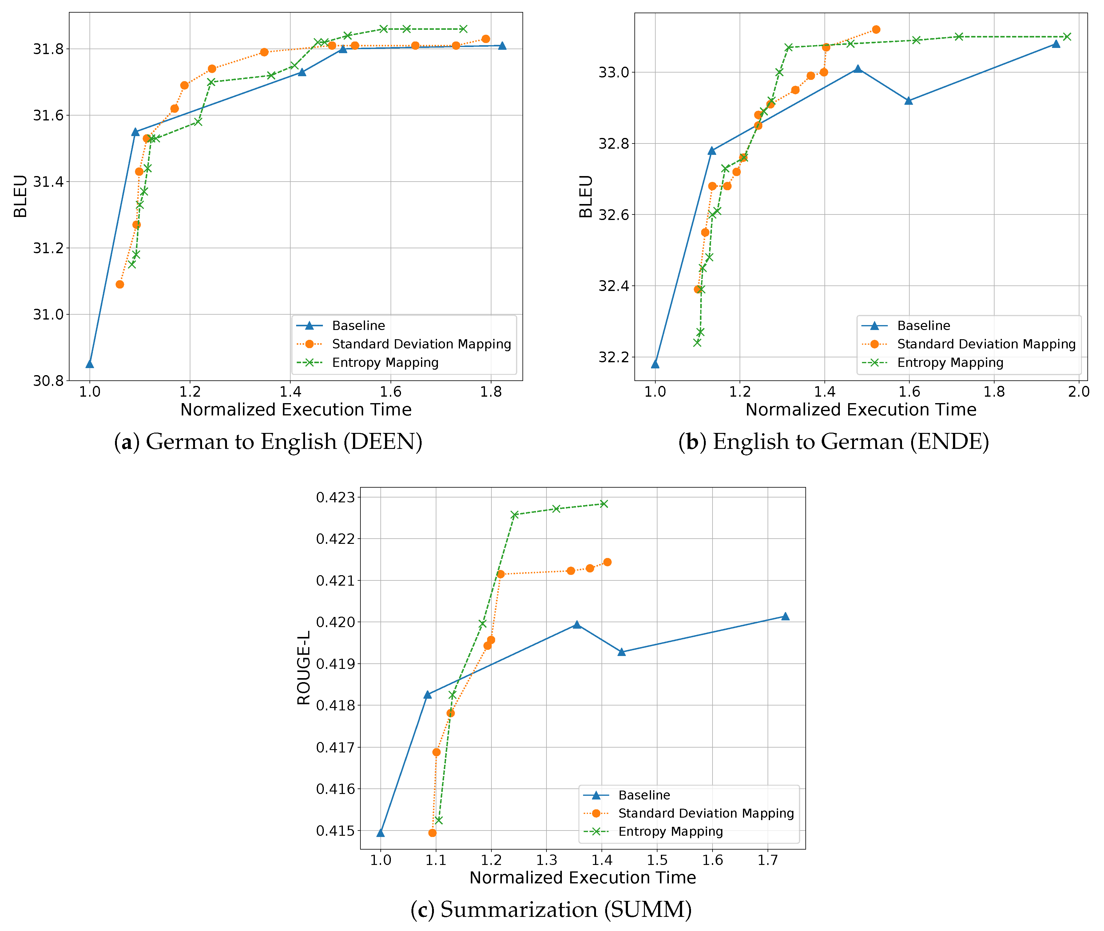
In this section, we compare static and dynamic beam search in terms of accuracy (measured by the BLEU and ROUGE scores, depending on the application) and execution time. To that end, we have run a dynamic beam search on the embedded board with both mapping policies, using the hyper-parameters selected as Pareto points in Section 4.2. For each point, we have measured the average execution time per sentence and the corresponding average score (BLEU/ROUGE). The results of this analysis are reported in Figure 11. For comparison, the figure also reports the baseline results obtained with a fixed BW (varied from 1 to 5 for all three networks). All time values are normalized to the average execution time of one sentence using a fixed BW=1, in order to make our results less device-dependent.
The figure shows the two main advantages of dynamic beam search. First, it greatly enriches the set of possible complexity-accuracy points that can be selected by a designer implementing sequence-to-sequence models on embedded devices. Importantly, these points can also be easily switched at runtime (e.g., depending on the available battery charge), by simply replacing the parameters of the BW mapping policy, which are passed as inputs to the inference function. Second, in some conditions, a dynamic beam search allows one to greatly reduce the average execution time per sentence without reducing the output quality. This is particularly evident for the SUMM network, where our dynamic beam search greatly outperforms the static solution, but it also applies to the other two models. For example, on DEEN we are able to reduce the inference time up to 20% while maintaining the same BLEU score achieved with a fixed BW of 5. On ENDE, the same BLEU of a static BW of five is obtained with a 25% execution time reduction. Note that the high ROUGE scores obtained with our technique on the SUMM network could also be obtained with a larger fixed BW value (>5), but such a large value would greatly increase the average inference time.
Figure 11 also shows that none of the two considered policies can outperform the baseline when BW < 2. This is in contrast with our previous results of [9], which however, were obtained on a different CPU architecture (not an embedded one), and was probably due to architecture-dependent optimizations performed by the underlying inference framework in the case of a fixed BW = 1. We did not investigate the reasons for this difference further, since one of our objectives was to develop a technique orthogonal to the inference framework (which was used without modifications in all our experiments); hence, those types of optimization are out of the scope of this work.
Finally, the graphs also show that the two BW mapping policies perform very similarly, and that despite being heuristic, the standard deviation mapping sometimes outperforms the entropy mapping. The differences between the two policies are data dependent, which means that the selections among the two should be done by empirically evaluating their respective performances on the target dataset.

4.5. Accuracy Versus Energy

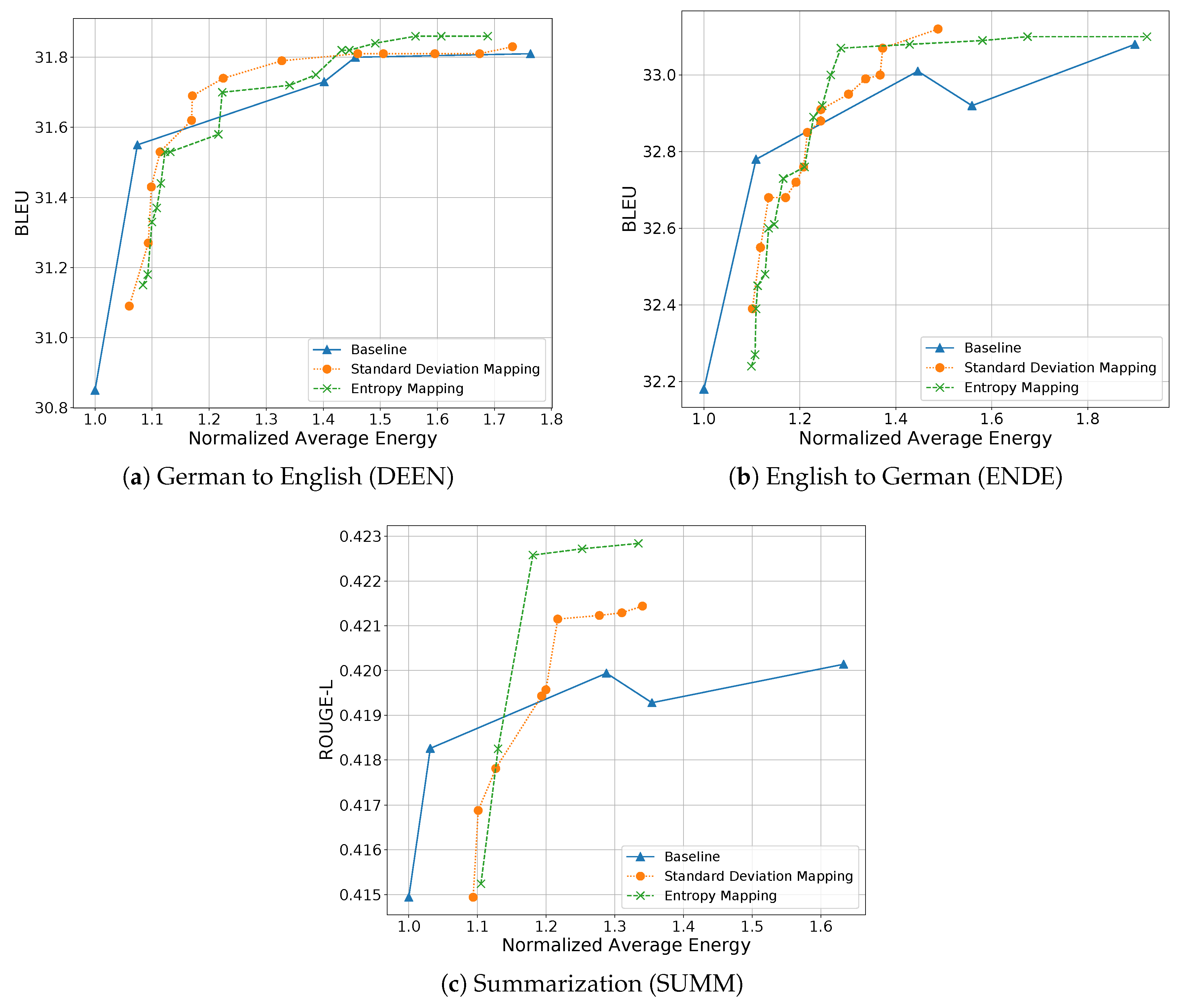
In this last experiment, we analyze the trade-off between model accuracy and energy consumption. Figure 12 shows the results of the same experiment of Figure 11 but reporting on the x-axis the normalized energy per sentence rather than the execution time. The resulting trade-offs are almost identical to those of Figure 11, as expected given the analysis of Section 4.3. Indeed, these plots simply confirm that, regardless of the policy and hyper-parameters, time and energy remain proportional, or in other words, that power remains constant throughout the inference process. All considerations done in Section 4.4 on the effectiveness of our proposed technique apply here as well.

5. Conclusions

We have proposed a novel, dynamic optimization technique for sequence-to-sequence deep neural networks, called dynamic beam search, which is based on tuning the beam width at each decoding step, depending on the difficulty of the processed sequence. Through the application of this technique, we have shown that the average inference execution time and energy consumption can be simultaneously reduced by up to 25% with no loss in output quality, when inference is performed on a single-core embedded device. In the future, we plan on studying the effectiveness of this approach in combination with other types of optimization, such as quantization.

Author Contributions

All authors have contributed equally to the paper. All authors have read and agreed to the published version of the manuscript.

Funding

This research received no external funding.

Conflicts of Interest

The authors declare no conflict of interest.

Abbreviations

The following abbreviations are used in this manuscript:
NMTneural machine translation
IoTInternet of Things
NNneural networks
Encencoder
Decdecoder
RNNrecurrent neural network
GRUgated recurrent unit
LSTMlong-short term memory
TCNtemporal convolutional network
EOSend Of sentence
BWbeam width
FPGAfield-programmable gate array
ASICapplication-specific integrated circuit
CNNconvolutional neural network
MPUmicroprocessing unit
MCUmicrocontroller unit
SIMDsingle-instruction multiple-data
GPUgraphical processing unit
CPUcentral processing unit
BLEUbilingual evaluation understudy
ROUGErecall-oriented understudy for Gisting evaluation
DSEdesign space exploration
DEENGerman to English network
ENDEEnglish to German network
SUMMEnglish summarization network

References

  1. LeCun, Y.; Bengio, Y.; Hinton, G. Deep Learning; The MIT Press: Cambridge, MA, USA, 2006. [Google Scholar]
  2. Vaswani, A.; Shazeer, N.; Parmar, N.; Uszkoreit, J.; Jones, L.; Gomez, A.N.; Kaiser, L.; Polosukhin, I. Attention Is All You Need. arXiv 2017, arXiv:1706.03762. [Google Scholar]
  3. Sze, V.; Chen, Y.H.; Yang, T.J.; Emer, J.S. Efficient Processing of Deep Neural Networks: A Tutorial and Survey. Proc. IEEE 2017, 105, 2295–2329. [Google Scholar] [CrossRef] [Green Version]
  4. Moons, B.; Verhelst, M. A 0.3-2.6 TOPS/W precision-scalable processor for real-time large-scale ConvNets. In Proceedings of the 2016 IEEE Symposium on VLSI Circuits (VLSI-Circuits), Honolulu, HI, USA, 15–17 June 2016; pp. 1–2. [Google Scholar] [CrossRef] [Green Version]
  5. Tann, H.; Hashemi, S.; Bahar, R.I.; Reda, S. Runtime configurable deep neural networks for energy-accuracy trade-off. In Proceedings of the Eleventh IEEE/ACM/IFIP International Conference on Hardware/Software Codesign and System Synthesis—CODES ’16, New York, NY, USA, 1–7 October 2016; pp. 1–10. [Google Scholar] [CrossRef] [Green Version]
  6. Andri, R.; Cavigelli, L.; Rossi, D.; Benini, L. YodaNN: An ultra-low power convolutional neural network accelerator based on binary weights. In Proceedings of the IEEE Computer Society Annual Symposium on VLSI (ISVLSI), Pittsburgh, PA, USA, 11–13 July 2016; pp. 236–241. [Google Scholar] [CrossRef]
  7. Guo, Y.; Yao, A.; Chen, Y. Dynamic Network Surgery for Efficient DNNs. arXiv 2016, arXiv:1608.04493. [Google Scholar]
  8. Jahier Pagliari, D.; Macii, E.; Poncino, M. Dynamic Bit-width Reconfiguration for Energy-Efficient Deep Learning Hardware. In Proceedings of the International Symposium on Low Power Electronics and Design (ISLPED ’18), Seattle, WA, USA, 23–25 July 2018; ACM: New York, NY, USA, 2018; pp. 47:1–47:6. [Google Scholar] [CrossRef]
  9. Jahier Pagliari, D.; Panini, F.; Macii, E.; Poncino, M. Dynamic Beam Width Tuning for Energy-Efficient Recurrent Neural Networks. In Proceedings of the 2019 on Great Lakes Symposium on VLSI (GLSVLSI ’19), Tysons Corner, VA, USA, 9–11 May 2019; ACM: New York, NY, USA, 2019; pp. 69–74. [Google Scholar] [CrossRef]
  10. Silfa, F.; Dot, G.; Arnau, J.M.; Gonzalez, A. E-PUR: An Energy-Efficient Processing Unit for Recurrent Neural Networks. In Proceedings of the 27th International Conference on Parallel Architectures and Compilation Techniques (PACT ’18), Limassol, Cyprus, 1–4 November 2018; ACM: New York, NY, USA, 2018; pp. 1–12. [Google Scholar] [CrossRef] [Green Version]
  11. Park, E.; Kim, D.; Kim, S.; Kim, Y.D.; Kim, G.; Yoon, S.; Yoo, S. Big/little deep neural network for ultra low power inference. In Proceedings of the 2015 International Conference on Hardware/Software Codesign and System Synthesis (CODES+ISSS), Amsterdam, The Netherlands, 4–9 October 2015; pp. 124–132. [Google Scholar] [CrossRef]
  12. Chen, X.; Mao, J.; Gao, J.; Nixon, K.W.; Chen, Y. MORPh. In Proceedings of the 53rd Annual Design Automation Conference on—DAC ’16, Austin, TX, USA, 5–9 June 2016; ACM Press: New York, NY, USA, 2016; pp. 1–6. [Google Scholar] [CrossRef]
  13. Sun, F.; Lin, J.; Wang, Z. Intra-layer Nonuniform Quantization for Deep Convolutional Neural Network. arXiv 2016, arXiv:1607.02720. [Google Scholar]
  14. Yang, T.; Chen, Y.; Sze, V. Designing Energy-Efficient Convolutional Neural Networks Using Energy-Aware Pruning. In Proceedings of the 2017 IEEE Conference on Computer Vision and Pattern Recognition (CVPR), Honolulu, HI, USA, 21–26 July 2017; pp. 6071–6079. [Google Scholar] [CrossRef] [Green Version]
  15. Gao, C.; Neil, D.; Ceolini, E.; Liu, S.C.; Delbruck, T. DeltaRNN: A Power-efficient Recurrent Neural Network Accelerator. In Proceedings of the 2018 ACM/SIGDA International Symposium on Field-Programmable Gate Arrays (FPGA ’18), Monterey, CA, USA, 25–27 February 2018; pp. 21–30. [Google Scholar] [CrossRef] [Green Version]
  16. Zhang, C.; Li, P.; Sun, G.; Guan, Y.; Xiao, B.; Cong, J. Optimizing FPGA-based Accelerator Design for Deep Convolutional Neural Networks. In Proceedings of the 2015 ACM/SIGDA International Symposium on Field-Programmable Gate Arrays (FPGA ’15), Monterey, CA, USA, 22–24 February 2015; ACM: New York, NY, USA, 2015; pp. 161–170. [Google Scholar] [CrossRef]
  17. Shi, R.; Liu, J.; So, H.K.H.; Wang, S.; Liang, Y. E-LSTM: Efficient Inference of Sparse LSTM on Embedded Heterogeneous System. In Proceedings of the 56th Annual Design Automation Conference 2019 (DAC ’19), Las Vegas NV USA, 3–6 June 2019; ACM: New York, NY, USA, 2019; pp. 182:1–182:6. [Google Scholar] [CrossRef]
  18. Kung, J.; Park, J.; Park, S.; Kim, J.J. Peregrine: A Flexible Hardware Accelerator for LSTM with Limited Synaptic Connection Patterns. In Proceedings of the 56th Annual Design Automation Conference 2019 (DAC ’19), Las Vegas NV USA, 3–6 June 2019; ACM: New York, NY, USA, 2019; pp. 209:1–209:6. [Google Scholar] [CrossRef]
  19. Cao, S.; Zhang, C.; Yao, Z.; Xiao, W.; Nie, L.; Zhan, D.; Liu, Y.; Wu, M.; Zhang, L. Efficient and Effective Sparse LSTM on FPGA with Bank-Balanced Sparsity. In Proceedings of the 2019 ACM/SIGDA International Symposium on Field-Programmable Gate Arrays (FPGA ’19), Seaside, CA, USA, 24–26 February 2019; ACM: New York, NY, USA, 2019; pp. 63–72. [Google Scholar] [CrossRef]
  20. Moons, B.; Brabandere, B.D.; Gool, L.V.; Verhelst, M. Energy-efficient ConvNets through approximate computing. In Proceedings of the 2016 IEEE Winter Conference on Applications of Computer Vision (WACV), Lake Placid, NY, USA, 7–10 March 2016; pp. 1–8. [Google Scholar] [CrossRef] [Green Version]
  21. Hubara, I.; Courbariaux, M.; Soudry, D.; El-Yaniv, R.; Bengio, Y. Binarized Neural Networks. In Advances in Neural Information Processing Systems 29; Lee, D.D., Sugiyama, M., Luxburg, U.V., Guyon, I., Garnett, R., Eds.; Curran Associates, Inc.: Red Hook, NY, USA, 2016; pp. 4107–4115. [Google Scholar]
  22. Amoh, J.; Odame, K. An Optimized Recurrent Unit for Ultra-Low-Power Keyword Spotting. arXiv 2019, arXiv:1902.05026. [Google Scholar] [CrossRef] [Green Version]
  23. Jahier Pagliari, D.; Poncino, M. Application-Driven Synthesis of Energy-Efficient Reconfigurable-Precision Operators. In Proceedings of the 2018 IEEE International Symposium on Circuits and Systems (ISCAS), Florence, Italy, 27–30 May 2018; pp. 1–5. [Google Scholar] [CrossRef]
  24. Panda, P.; Sengupta, A.; Roy, K. Conditional Deep Learning for Energy-Efficient and Enhanced Pattern Recognition. In Proceedings of the 2016 Conference on Design, Automation & Test in Europe (DATE ’16), Dresden, Germany, 14–18 March 2016; EDA Consortium: San Jose, CA, USA, 2016; pp. 475–480. [Google Scholar]
  25. Parsa, M.; Panda, P.; Sen, S.; Roy, K. Staged Inference using Conditional Deep Learning for energy efficient real-time smart diagnosis. In Proceedings of the 2017 39th Annual International Conference of the IEEE Engineering in Medicine and Biology Society (EMBC), Jeju Island, Korea, 11–15 July 2017; pp. 78–81. [Google Scholar] [CrossRef]
  26. Moons, B.; Uytterhoeven, R.; Dehaene, W.; Verhelst, M. Envision: A 0.26-to-10TOPS/W subword-parallel dynamic-voltage-accuracy-frequency-scalable Convolutional Neural Network processor in 28nm FDSOI. In Proceedings of the 2017 IEEE International Solid-State Circuits Conference (ISSCC), San Francisco, CA, USA, 5–9 February 2017; pp. 246–247. [Google Scholar] [CrossRef]
  27. Yan, Z.; Zhang, H.; Piramuthu, R.; Jagadeesh, V.; DeCoste, D.; Di, W.; Yu, Y. HD-CNN: Hierarchical Deep Convolutional Neural Networks for Large Scale Visual Recognition. In Proceedings of the 2015 IEEE International Conference on Computer Vision (ICCV), Santiago, Chile, 11–18 December 2015; pp. 2740–2748. [Google Scholar] [CrossRef] [Green Version]
  28. Moons, B.; Uytterhoeven, R.; Dehaene, W.; Verhelst, M. DVAFS: Trading computational accuracy for energy through dynamic-voltage-accuracy-frequency-scaling. In Proceedings of the Design, Automation Test in Europe Conference Exhibition (DATE), Lausanne, Switzerland, 27–31 March 2017; pp. 488–493. [Google Scholar] [CrossRef]
  29. Freitag, M.; Al-Onaizan, Y. Beam search strategies for neural machine translation. arXiv 2017, arXiv:1702.01806. [Google Scholar]
  30. Branke, J.; Branke, J.; Deb, K.; Miettinen, K.; Slowiński, R. Multiobjective Optimization: Interactive and Evolutionary Approaches; Springer Science & Business Media: Berlin/Heidelberg, Germany, 2008; Volume 5252. [Google Scholar]
  31. Goodfellow, I.; Bengio, Y.; Courville, A. Deep Learning; The MIT Press: Cambridge, MA, USA, 2016. [Google Scholar]
  32. Cettolo, M.; Niehues, J.; Stüker, S.; Bentivogli, L.; Federico, M. Report on the 11th IWSLT evaluation campaign, IWSLT 2014. In Proceedings of the International Workshop on Spoken Language Translation, South Lake Tahoe, CA, USA, 4–5 December 2014; p. 57. [Google Scholar]
  33. Bojar, O.; Buck, C.; Federmann, C.; Haddow, B.; Koehn, P.; Leveling, J.; Monz, C.; Pecina, P.; Post, M.; Saint-Amand, H.; et al. Findings of the 2014 Workshop on Statistical Machine Translation. In Proceedings of the Ninth Workshop on Statistical Machine Translation, Baltimore, MD, USA, 26–27 June 2014; Association for Computational Linguistics: Stroudsburg, PA, USA, 2014; pp. 12–58. [Google Scholar]
  34. Graff, D.; Kong, J.; Chen, K.; Maeda, K. English gigaword. Linguist. Data Consort. Phila. 2003, 4, 34. [Google Scholar]
  35. Matuszewski, J.; Pietrow, D. Recognition of electromagnetic sources with the use of deep neural networks. In Proceedings of the XII Conference on Reconnaissance and Electronic Warfare Systems, Ołtarzew, Poland, 19–21 November 2018; Kaniewski, P., Ed.; International Society for Optics and Photonics: San Diego, CA, USA, 2018; Volume 11055, pp. 100–114. [Google Scholar] [CrossRef]
  36. Matuszewski, J. Radar signal identification using a neural network and pattern recognition methods. In Proceedings of the 2018 14th International Conference on Advanced Trends in Radioelecrtronics, Telecommunications and Computer Engineering (TCSET), Lviv-Slavske, Ukraine, 20–24 February 2018; pp. 79–83. [Google Scholar] [CrossRef]
  37. Dudczyk, J.; Kawalec, A. Adaptive Forming of the Beam Pattern of Microstrip Antenna with the Use of an Artificial Neural Network. Int. J. Antennas Propag. 2012, 2012. [Google Scholar] [CrossRef]
  38. Gehring, J.; Auli, M.; Grangier, D.; Yarats, D.; Dauphin, Y.N. Convolutional Sequence to Sequence Learning. arXiv 2017, arXiv:1705.03122. [Google Scholar]
  39. Zhang, Y.; Wang, C.; Gong, L.; Lu, Y.; Sun, F.; Xu, C.; Li, X.; Zhou, X. A Power-Efficient Accelerator Based on FPGAs for LSTM Network. In Proceedings of the 2017 IEEE International Conference on Cluster Computing (CLUSTER), Honolulu, HI, USA, 5–8 September 2017; pp. 629–630. [Google Scholar] [CrossRef]
  40. Chen, C.; Ding, H.; Peng, H.; Zhu, H.; Ma, R.; Zhang, P.; Yan, X.; Wang, Y.; Wang, M.; Min, H.; et al. OCEAN: An on-chip incremental-learning enhanced processor with gated recurrent neural network accelerators. In Proceedings of the ESSCIRC 2017—43rd IEEE European Solid State Circuits Conference, Leuven, Belgium, 11–14 September 2017; pp. 259–262. [Google Scholar] [CrossRef]
  41. Lee, J.; Shin, D.; Yoo, H.J. A 21mW low-power recurrent neural network accelerator with quantization tables for embedded deep learning applications. In Proceedings of the 2017 IEEE Asian Solid-State Circuits Conference (A-SSCC), Seoul, Korea, 6–8 November 2017; pp. 237–240. [Google Scholar] [CrossRef]
  42. Lin, D.D.; Talathi, S.S.; Annapureddy, V.S. Fixed Point Quantization of Deep Convolutional Networks. In Proceedings of the International Conference on Machine Learning, Lille, France, 6–11 July 2015; Volume 48, pp. 2849–2858. [Google Scholar]
  43. Hashemi, S.; Anthony, N.; Tann, H.; Bahar, R.I.; Reda, S. Understanding the Impact of Precision Quantization on the Accuracy and Energy of Neural Networks. In Proceedings of the Design, Automation & Test in Europe Conference & Exhibition (DATE), Lausanne, Switzerland, 27–31 March 2017; pp. 1474–1479. [Google Scholar] [CrossRef] [Green Version]
  44. Courbariaux, M.; Hubara, I.; Soudry, D.; El-Yaniv, R.; Bengio, Y. Binarized Neural Networks: Training Deep Neural Networks with Weights and Activations Constrained to +1 or −1. arXiv 2016, arXiv:1602.02830. [Google Scholar]
  45. Jahier Pagliari, D.; Poncino, M.; Macii, E. Energy-Efficient Digital Processing via Approximate Computing. In Smart Systems Integration and Simulation; Bombieri, N., Poncino, M., Pravadelli, G., Eds.; Springer International Publishing: Cham, Switzerlands, 2016; Chapter 4; pp. 55–89. [Google Scholar] [CrossRef]
  46. Ott, J.; Lin, Z.; Zhang, Y.; Liu, S.C.; Bengio, Y. Recurrent Neural Networks With Limited Numerical Precision. arXiv 2016, arXiv:1611.07065. [Google Scholar]
  47. Hubara, I.; Courbariaux, M.; Soudry, D.; El-Yaniv, R.; Bengio, Y. Quantized Neural Networks: Training Neural Networks with Low Precision Weights and Activations. arXiv 2016, arXiv:1609.07061. [Google Scholar]
  48. Molchanov, P.; Tyree, S.; Karras, T.; Aila, T.; Kautz, J. Pruning Convolutional Neural Networks for Resource Efficient Inference. arXiv 2016, arXiv:1611.06440. [Google Scholar]
  49. Lai, L.; Suda, N.; Chandra, V. CMSIS-NN: Efficient Neural Network Kernels for Arm Cortex-M CPUs. arXiv 2018, arXiv:1801.06601. [Google Scholar]
  50. Garofalo, A.; Rusci, M.; Conti, F.; Rossi, D.; Benini, L. PULP-NN: Accelerating quantized neural networks on parallel ultra-low-power RISC-V processors. Philos. Trans. R. Soc. Math. Phys. Eng. Sci. 2020, 378, 20190155. [Google Scholar] [CrossRef] [PubMed] [Green Version]
  51. Devlin, J.; Chang, M.W.; Lee, K.; Toutanova, K. BERT: Pre-training of Deep Bidirectional Transformers for Language Understanding. arXiv 2018, arXiv:1810.04805. [Google Scholar]
  52. Radford, A.; Narasimhan, K.; Salimans, T.; Sutskever, I. Improving Language Understanding by Generative Pre-Training. Available online: https://openai.com/blog/language-unsupervised/ (accessed on 6 February 2020).
  53. Abadi, M.; Agarwal, A.; Barham, P.; Brevdo, E.; Chen, Z.; Citro, C.; Corrado, G.S.; Davis, A.; Dean, J.; Devin, M.; et al. Tensorflow: Large-scale machine learning on heterogeneous distributed systems. arXiv 2016, arXiv:1603.04467. [Google Scholar]
  54. Paszke, A.; Gross, S.; Massa, F.; Lerer, A.; Bradbury, J.; Chanan, G.; Killeen, T.; Lin, Z.; Gimelshein, N.; Antiga, L.; et al. PyTorch: An imperative style, high-performance deep learning library. In Proceedings of the Advances in Neural Information Processing Systems (NIPS 2019), Vancouver, BC, Canada, 8–14 December 2019; pp. 8024–8035. [Google Scholar]
  55. Klein, G.; Kim, Y.; Deng, Y.; Senellart, J.; Rush, A. OpenNMT: Open-Source Toolkit for Neural Machine Translation. In Proceedings of the 55th Annual Meeting of the Association for Computational Linguistics (ACL) 2017, System Demonstrations, Vancouver, BC, Canada, 30 July–4 August 2017; pp. 67–72. [Google Scholar]
  56. Papineni, K.; Roukos, S.; Ward, T.; Zhu, W.J. BLEU: a method for automatic evaluation of machine translation. In Proceedings of the 40th Annual Meeting on Association for Computational Linguistics (ACL), Philadelpha, PA, USA, 7–12 July 2002; pp. 311–318. [Google Scholar]
  57. Lin, C.Y. Rouge: A Package for Automatic Evaluation of Summaries; Text Summarization Branches Out; Association for Computational Linguistics: Barcelona, Spain, 2004; pp. 74–81. [Google Scholar]
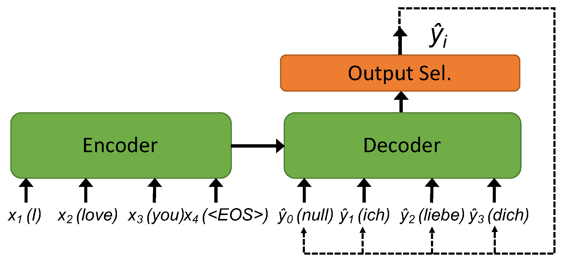
Figure 1. Architecture of an encoder-decoder sequence-to-sequence neural network.
Electronics 09 00337 g001
Figure 2. Operation of the decoder network during the inference phase when using a greedy search algorithm.
Electronics 09 00337 g002
Figure 3. Operation of the decoder network during the inference phase when using a beam search algorithm with B W = 3 .
Electronics 09 00337 g003
Figure 4. Normalized inference time for different fixed beam width values on an embedded device.
Electronics 09 00337 g004
Figure 5. Average power per input sequence with different fixed Beam Width values during inference on an embedded device.
Electronics 09 00337 g005
Figure 6. A high level overview of dynamic beam search.
Electronics 09 00337 g006
Figure 7. Linear mapping from the entropy of the decoder output probabilities to the selected beam width.
Electronics 09 00337 g007
Figure 8. Linear mapping from the standard deviation of the top-k output probabilities to the selected beam width.
Electronics 09 00337 g008
Figure 9. Proposed method for hyper-parameter tuning.
Electronics 09 00337 g009
Figure 10. Average power per input sequence with different fixed beam width values and with a varying beam width set according to our proposed technique.
Electronics 09 00337 g010
Figure 11. Translation/summarization accuracy (measured by BLEU and ROUGE scores respectively) versus normalized execution time for the three target models using either static or dynamic beam search.
Electronics 09 00337 g011
Figure 12. Translation/summarization accuracy (measured by BLEU and ROUGE scores respectively) versus normalized energy for the three target models using either static or dynamic beam search.
Electronics 09 00337 g012
Table 1. Design space exploration statistics for the three target models.
ModelTotal DSE Time [H]Total Points TestedPareto Points SelectedReduction
DEEN202001712x
ENDE602001712x
SUMM72001315x
Table 2. Execution time statistics for the two proposed BW mapping policies.
ModelPolicyMin. [s]Max. [s]Median [s]
DEENEntropy0.00540.02760.0165
Std. Dev.0.00100.014580.0053
ENDEEntropy0.00680.03450.0209
Std. Dev.0.00110.01800.0068
SUMMEntropy0.01060.05570.0326
Std. Dev.0.00180.03020.0112
Table 3. Policy parameters used for the plots of Figure 10.
ModelBWminBWmaxCoeff.Intercept
DEEN121.10.5
ENDE1240.5
SUMM140.30.3