Open Vision System for Low-Cost Robotics Education

Abstract

Vision devices are currently one of the most widely used sensory elements in robots: commercial autonomous cars and vacuum cleaners, for example, have cameras. These vision devices can provide a great amount of information about robot surroundings. However, platforms for robotics education usually lack such devices, mainly because of the computing limitations of low cost processors. New educational platforms using Raspberry Pi are able to overcome this limitation while keeping costs low, but extracting information from the raw images is complex for children. This paper presents an open source vision system that simplifies the use of cameras in robotics education. It includes functions for the visual detection of complex objects and a visual memory that computes obstacle distances beyond the small field of view of regular cameras. The system was experimentally validated using the PiCam camera mounted on a pan unit on a Raspberry Pi-based robot. The performance and accuracy of the proposed vision system was studied and then used to solve two visual educational exercises: safe visual navigation with obstacle avoidance and person-following behavior.

1. Introduction

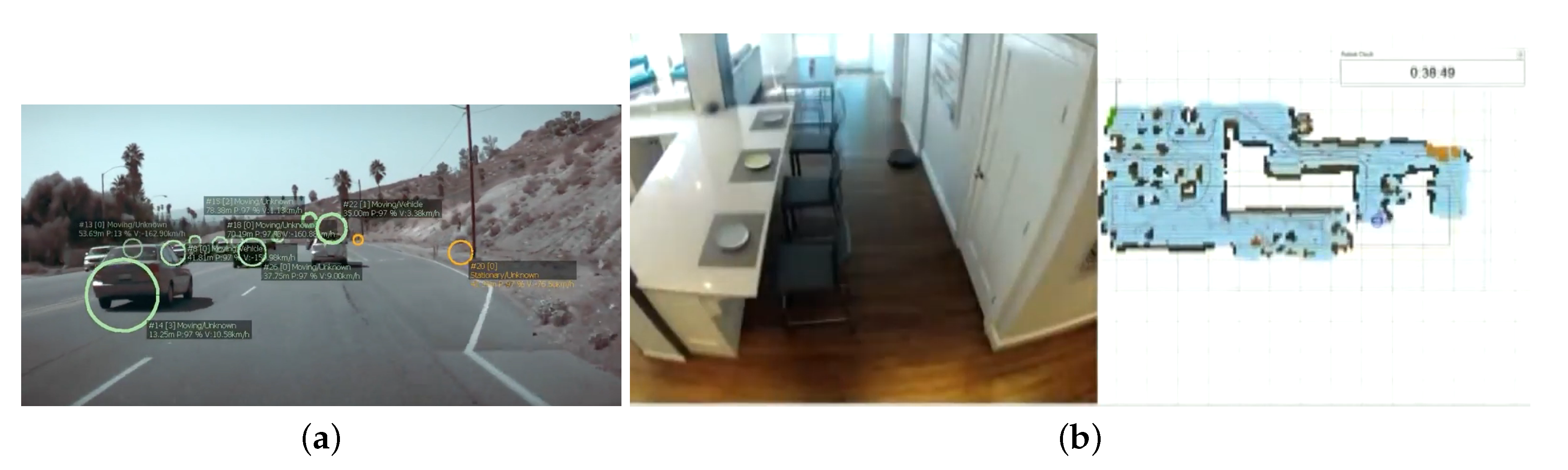
Computer vision is a fast-growing field, both in robotics and in many other applications, from surveillance systems for security to the automatic acquisition of 3D models for Virtual Reality displays. The number of commercial applications is increasing; examples include traffic monitoring, parking entry control, augmented reality videogames and face recognition. In addition, vision is one of the most successful sensing modalities used in real robots, such as cars with the semi-autonomous Tesla AutoPilot driving system (Figure 1a), the best Roomba vacuum cleaner models (Figure 1b) and packaging robots.

In recent years, cameras have been included as common sensory equipment in robots. As sensors, they are economical and able to provide robots with extensive information about their environment. As in humans, vision appears to be the most effective sensor system for robots. However, extracting the required information from the image flow is not easy, and has certain limitations such as the small field of view of conventional cameras or scenarios with poor lighting conditions.

Typically, vision has been used in robotics for navigation, object recognition and tracking, 3D mapping, visual attention, self-localization, etc. Cameras may be used to detect and track relevant objects for the task in which the robot is currently engaged. They can provide the most complete information about the objects around the robot and their location. Moreover, with active cameras, it is possible to revisit features of a previously visited area, even if the area is out of immediate visual range. In order to have access to accurate information about the areas of interest that surround the robot, a detailed memory map of the environment can be created [1]. Since the computational cost of maintaining such an amount of information is high, only a few object references can be maintained; for instance, the learning procedure could be performed by an SVM classifier able to accurately recognize multiple dissimilar places [2].

On occasions, the data flow from a camera is overwhelming [3] and a number of attention mechanisms have been developed to focus on the relevant visual stimuli. Humans have a precise natural active vision system [4,5,6], which means that we can concentrate on certain regions of interest in the scene around us, thanks to the movement of our eyes and/or head, or simply by distributing the gaze across different zones within the image that we are perceiving [7], extracting information features from the scene [8]. One advantage compared to the passive approach, where visual sensors are static and all parts of the images are equally inspected, is that parts of a scene that are perhaps inaccessible to a static sensor can be seen by a moving device, is similar to how the moving eyes and head of humans provide an almost complete panoramic range of view.

Given that robots are generally required to navigate autonomously through dynamic environments, their visual system can be used to detect and avoid obstacles [9,10]. When using cameras, obstacles can be detected through 3D reconstruction. Thus, the recovery of three-dimensional information has been the main focus of the computer vision community for decades [11], although Remazeilles et al. [12] presented a solution that does not require 3D reconstruction.

Other relevant information that can be extracted from the images is the self-localization of the robot [10]. Robots need to know their location within the environment in order to develop an appropriate behavior [13]. Using vision and a map, the robot can estimate its own position and orientation within a known environment [14]. The auto-location of robots has proven to be complex, especially in dynamic environments and those with a high degree of symmetry, where the values of the sensors can be similar in different positions [15]. In addition, many recent visualSLAM techniques [16] have successfully provided a solution for simultaneous mapping and localization.

Despite the widespread use of cameras in commercial robots, very few educational robot platforms and frameworks use cameras. This is mainly because of the high computing power required for image processing. The standard low-cost processors in educational robots like, for example, Arduino-based robots, do not have sufficient computing speed for this. Another reason is that image processing is not simple and the required complexity typically exceeds the capabilities of children and young students. Nevertheless, cameras have a promising future and it is thus desirable to expose students to computer vision in robotics.

Robotics educational kits typically include the hardware components needed to build the robot (sensors, motors, small computer) and a programming framework specific to that robot, possibly a text-based or graphic language, such as Scratch. They are interesting tools to enrich students’ education and provide a motivating introduction to science and technology.

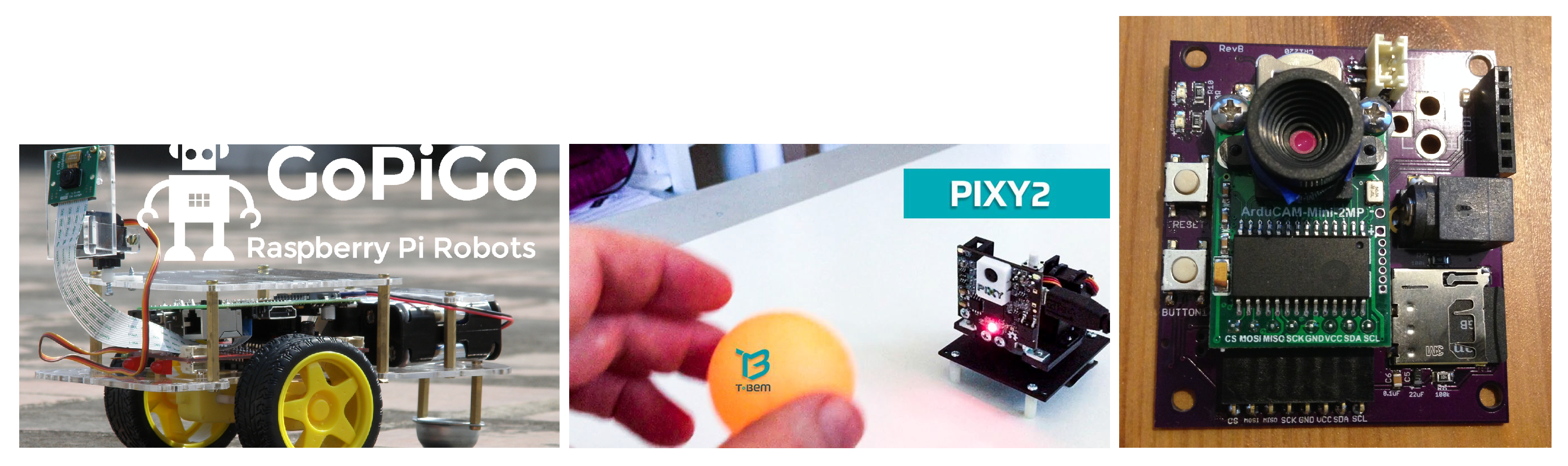
Current technological advances have provided low-cost robots with a sufficiently powerful processor (in terms of computing) to support image processing techniques. Raspberry Pi-based robots, a widespread example, include a bus (SCI) to transmit the data flow from their own PiCam camera, which is powerful, has good resolution, and makes little noise.

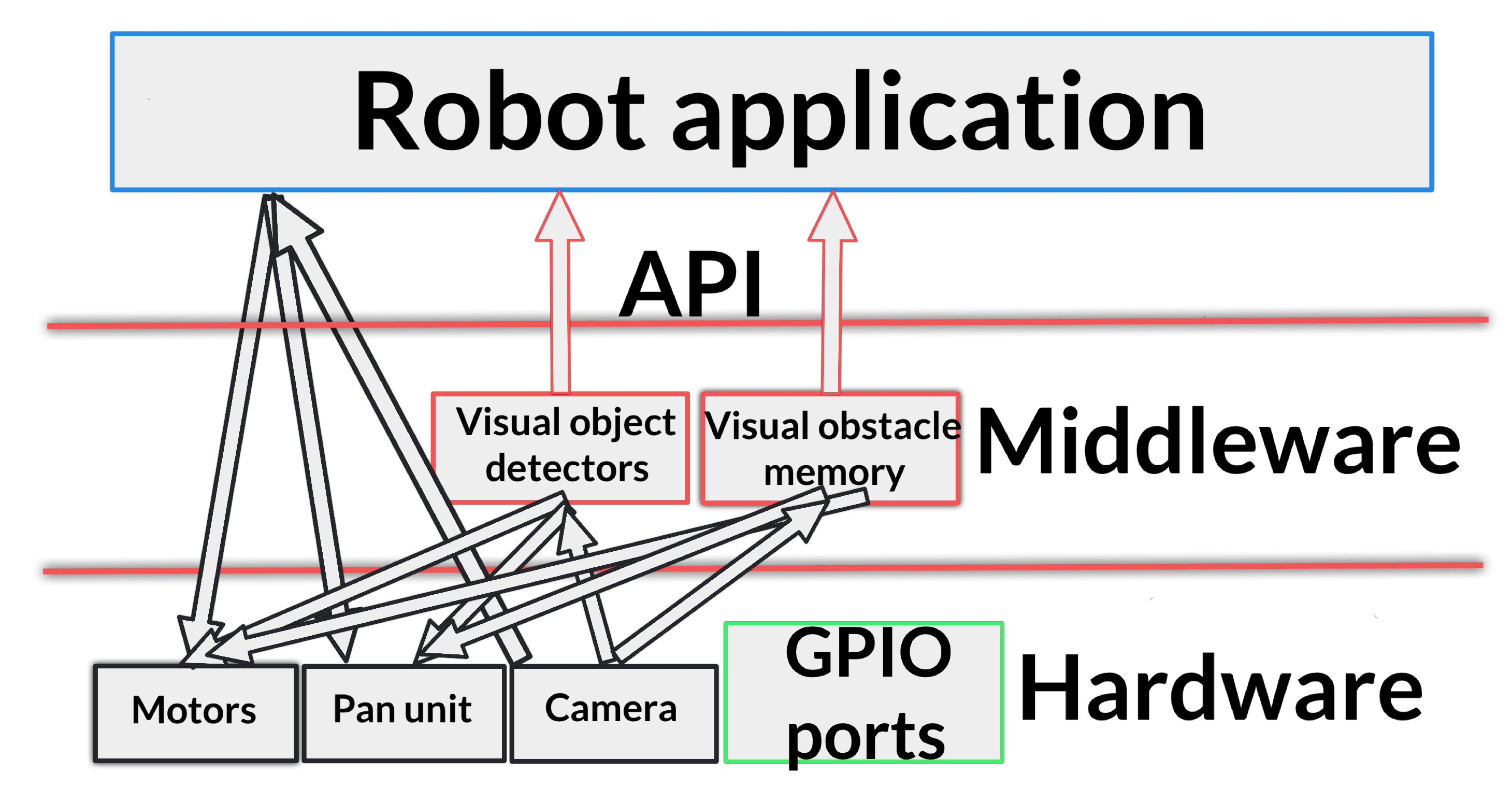
The proposed open vision system was created to improve educational robotics frameworks including an easy way to deal with vision, and robots with cameras. It is provided as a high-level library implemented in Python language. Several functions of the library extract information from the images. They mitigate the complexity of dealing with raw images and the robot application provides an abstract and simple way to use them. In particular, the proposed system offers two major contributions: a visual memory with information about obstacles, which allows the robot to navigate safety, and visual detectors of complex objects, such as human faces, which facilitate natural tracking and following behaviors. Using this system, students’ initial contact with vision is simple and enjoyable. It also expands the number of robot programming exercises, which can now involve the use of cameras.

2. Related Works

Many issues have been addressed in the intersection of computer vision and robotics: vision-based control or navigation, vision-based map building and 3D representation, vision-based localization, object recognition, attention and gaze control among others. Studies have recently emerged on vision in education. The most significant examples related to these issues are described below.

2.1. Vision in Education

In recent years, with the emergence of cards, such as Raspberry Pi, with more agile and advanced processors, vision algorithms can be transferred to robots to provide an educational approach.

For example, GoPiGo, is a complete kit (Figure 2 left, https://www.dexterindustries.com/gopigo3) to build a robot car that already incorporates the Raspberry Pi with vision. PixyCam (Figure 2 middle, https://pixycam.com) is a fast vision sensor for DIY robotics, such as Arduino, Raspberry Pi and similar applications. It can learn an object easily just by pressing a button, and it is also capable of tracking hundreds of objects simultaneously, providing only the data that is of interest.

ArduCam (Figure 2 right, https://www.arducam.com) is an open-source project for the Arduino camera that dates back to 2012. It was the world’s first SPI camera for Arduino and filled the gap of a missing camera support in the Arduino ecosystem. It supports a wide variety of camera modules from 0.3–5 MP. In fact, the ArduCam is not limited to the Arduino platform, but also supports almost any hardware platforms as long as they have an I2C and SPI interface like Black Beagle Bone, Raspberry Pi, mbed, etc. In addition, this project has been extended to USB cameras which support 0.3–14 MP camera modules.

The literature includes several studies on educational robotics with vision. David et al. [17] suggest the use of Pi for practice sessions in most of the laboratory courses in the computer science engineering curriculum. Most laboratory courses are implemented in C, C++, and Java languages. Apart from the above-mentioned languages, which can be executed in Raspberry Pi, some laboratory courses make use of front end and back end tools. Standard computers and Pi have been compared for execution time, power consumption, and environmental effect. In all cases, the Pi presents great advantages over existing systems.

Adams et al. [18] propose a Raspberry Pi robot, the R-Pi, for CS educators, with uses ranging from teaching the language of assembly to using it as a multiprocessor. Mathematics educators have produced extensive literature on the use of pedagogical tools known as “manipulatives” that have been shown to be effective in leading students through a “concrete, representational, abstract” progression of understanding an abstract topic. Adams believes that by using the R-Pi as a manipulative, this same “concrete, representational, abstract” progression can be used to help CS students master many topics that are often taught as abstractions.

Other interesting publications exist in this regard. Balon et al. [19] describe the idea of using Raspberry Pi computers in high schools and higher education. Hoyo et al. [20] present a proposal on how to combine a set of software and hardware resources available in the literature to be used as a support for control engineering education. The Raspberry Pi board is used as a platform to exploit the different proposed concepts. SciPy, Matplotlib, and NumPy libraries, which are Python-based open-source libraries for scientific computing and graphical representation, are used to perform Matlab-like simulations and to implement classical control loops.

Numerous publications can be found in the recent literature [21,22,23] about the general treatment of images with reduced processing boards, where middle-school students learn how to program their own video representations using Python libraries running on the Raspberry Pi.

Finally, a new subject of much research is how to use deep learning techniques on embedded boards such as the Raspberry Pi or the new Jetson Nano. ElAarag et al. [24] present this approach in applying the deeper learning framework to an Operating Systems course, using the Raspberry Pi as a vehicle. A preliminary evaluation shows that the use of the Raspberry Pi provides a deeper learning environment that helps students learn how to learn by working collaboratively and to think critically to solve complex problems.

2.2. Vision-Based Navigation

Dimitrov et al. [25] present improvements in the autonomous navigation of the Rover of Autonomous Exploration of NASA (AERO) in terms of robustness and reliability of sample collection. The AERO is required to navigate a large outdoor area, find and collect several geological samples, and return to the home platform autonomously and using only technologies compatible with the space.

Matthias et al. [26] describe how an aerial microrobotic device can autonomously and visually describe a specific trajectory and at the same time build a three-dimensional map of the area over which it flies. The processor used is the same as that of a mobile phone, which due to its low weight is passively safe and can be deployed close to humans, for rescue tasks.

Tweddle et al. [27] present another use of a navigation system based on vision, and internationally recognized by researchers. This study describes the VERTIGO vision system, a hardware update to the SPHERES satellites that allows the investigation of navigation based on vision in the environment of 6 degrees of freedom and microgravity of the International Space Station (ISS). This vision system includes stereo cameras, designed to be used by researchers in numerous experiments.

Smith et al. [28] describe the weaknesses of a vision-based global navigation system. Their work also studies the incorporation of deep learning techniques into the system, and concludes that applying this novel system efficiently provides the global planning system with samples of the environment so that it can make more intelligent decisions. In particular, simulations and tests on a real mobile robot show that the number of samples obtained by deep learning can be reduced by an order of magnitude and navigation performance is preserved.

2.3. Visual Attention Systems

Visual attention has two clearly marked stages: the first, considered prior processing, is one in which objects with certain features within the visual field are extracted, and the second, called focused attention, consists of identifying these objects.

Robots’ cameras provide an extensive flow of data from which the interesting information must be selected and any information not of interest must be ignored. This is known as selective visual attention. There are two aspects of visual attention, the global (overt attention) and the local (covert attention). Local attention [29,30,31] consists of selecting within an image the data that interest us. Global attention consists of selecting objects of interest in the environment around the robot, beyond the current visual field, and directing the gaze towards them [32,33].

The visual representation of interesting objects in the vicinity of the robot can improve the quality of robot behavior, as well as the ability to handle more information when making decisions. This poses a problem when the objects are not in the immediate field of vision. To solve this problem, omnidirectional vision is used in some works [34]; in others, a normal camera and a global attention mechanism are used [30,35], which allow samples to be quickly taken from a very wide area of interest. The use of camera movement to facilitate the recognition of objects was proposed by Ballard et al. [36] and is used, for example, to distinguish between different shapes in the images [31].

In his thesis, Rodríguez–Sánchez [37] defined a biology-inspired model for the representation of forms that included intermediate layers of visual representation corresponding to the layers that exist in the natural visual cortex (Figure 3), something not previously explored in the literature, and which shows they have a direct impact on the selection of color and 2D shapes. Furthermore, their combination leads to the formation of selective neurons.

Two in-depth comparative studies [38,39] present different taxonomies of up to 65 models. These works provide a critical comparison of approaches, and their capacities and deficiencies. In particular, more than a dozen criteria derived from behavioral and computational studies are formulated for the qualitative comparison of care models. In addition, these works address several challenging problems presented by the models, including the biological plausibility of the calculations, the correlation with eye movement data-sets, ascending and descending dissociation, and the construction of meaningful performance measures.

3. Design of the Visual System

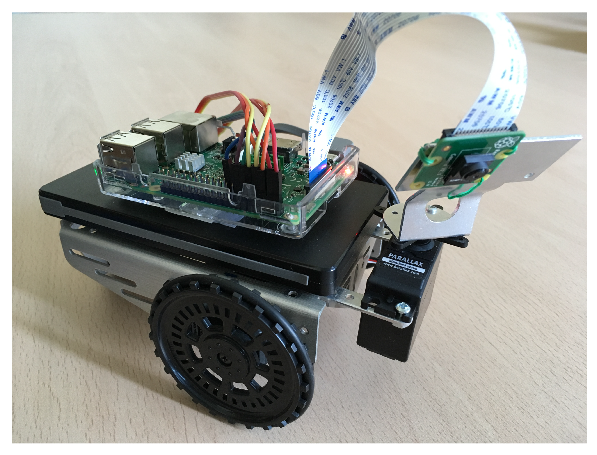
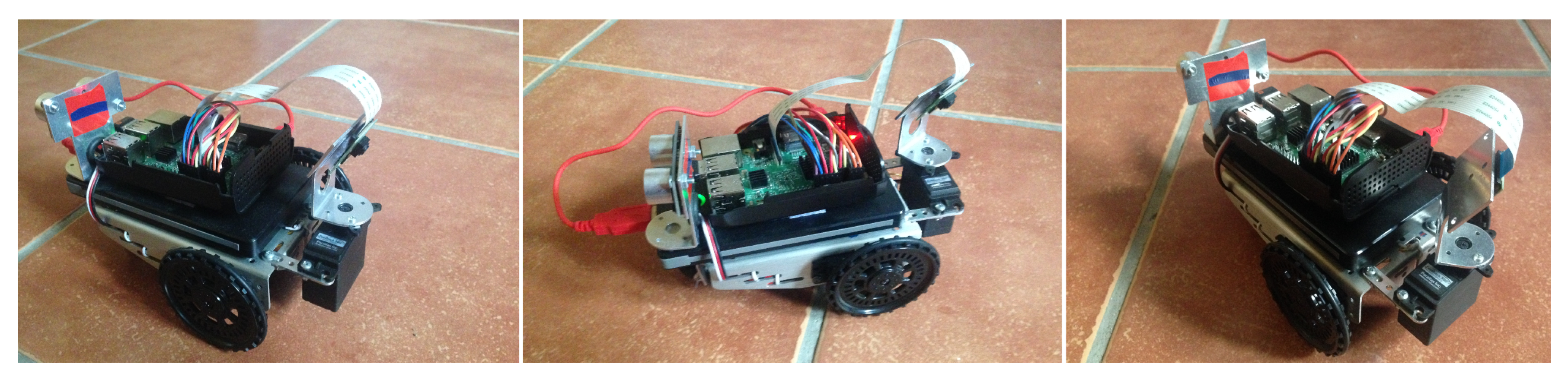
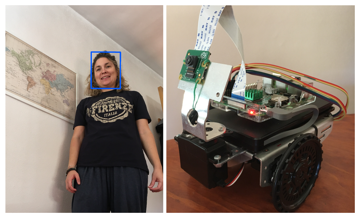
The perceptive system developed was tested on the robotic platform PiBot with its PiCamera mounted on a pan unit (Figure 4), which is based on the Raspberry Pi board [40]. It is designed, however, for any autonomous robots that use a single mobile camera, like that on the head of humanoids (e.g., Nao robots, used in the RoboCup competition) or in robots with pan-tilt units. It receives data from robot sensors (Figure 5), such as camera and encoders, and extracts refined information, such as the description of the objects around the robot or the robot position. This information is provided to other actuation components like the navigation algorithm or other control units. All the code is publicly available in its GitLab repository (https://gitlab.etsit.urjc.es/jmvega/pibot-vision).

The goal of the visual system is to create a local short-term visual memory to store and keep up-to-date basic information about objects in the scene surrounding the robot as well as to detect complex objects such as human faces.

The first stage of the system is 2D analysis, which detects 2D points corresponding to the bottom edges of objects. The 3D reconstruction algorithm then places these points in 3D space according to the ground-hypothesis; that is, we suppose that all objects are flat on the floor. Finally, the 3D memory system stores their position in 3D space.

In addition, the system has a complex object detector which detects, for example, human faces (https://gitlab.etsit.urjc.es/jmvega/pibot-vision/tree/master/followPerson). This feature of the visual system allows human faces around the scene to be tracked, and will be enhanced with new objects: traffic signals or face identity recognition, using new powerful hardware such as Jetson Nano.

In this section, we will see the various components of our implemented visual memory system, allowing the field of vision to be extended to the entire scene surrounding the robot, not just the immediate visual field.

4. Visual Memory

The goal of our visual memory is to store the information about the objects surrounding the robot, with a wide field of view perceived by the camera mounted over the pan unit.

4.1. 2D Image Processing

The first stage of the visual memory is a 2D analysis, which extracts 2D points as a basic primitive to obtain object contours (https://gitlab.etsit.urjc.es/jmvega/pibot-vision/tree/master/imageFilters). In prior implementations, the classic Canny edge filter was used, but it was too slow to run on this board, and insufficiently accurate and robust. Its outcomes tended not to be fully effective. Later, the Laplacian edge detector was used, improving the results.

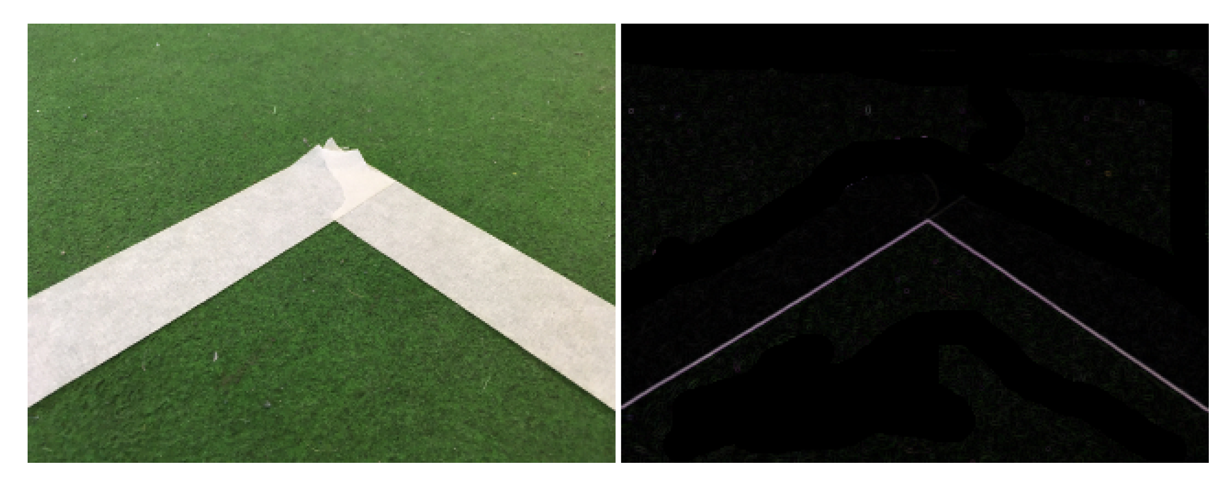
In the latest releases, this was replaced with its own simple algorithm, which consists of going through the image from bottom to top, by columns, from left to right. Then, the actual pixel is compared with an established color: it will be considered a border if it is of this color; otherwise, it will be ignored. The combination of colors on which the platform was tested corresponds to the real ones in the field used in the RoboCup: white lines on a green background (Figure 6).

Once the border is found, the algorithm stops and checks the next column of the image. This solution is surprisingly more accurate, more robust and faster, despite having fewer parameters for detecting edges.

4.2. Extracting 3D Edges

The above mechanism extracts a set of 2D points that must be located in 3D space. To do this, and as we have already mentioned, we rely on the idea of ground-hypothesis. Since we have one camera, we need a restriction which will enable the third dimension to be estimated. We assume that all objects are flat on the floor.

Once we have the corresponding 3D points, they are included in the 3D memory, shaping a visual sonar (https://gitlab.etsit.urjc.es/jmvega/pibot-vision/tree/master/projGeomLibrary). Figure 7 shows the 3D scene with edges reconstructed by the system, corresponding to the edges detected in the three snapshots.

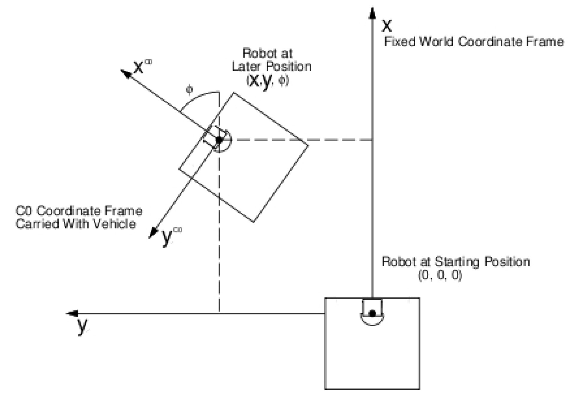
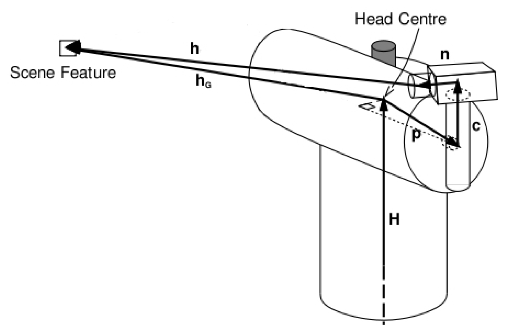
There are four key 3D coordinate systems in this approach. First, the absolute coordinate system, whose origin lies somewhere in the environment within which the robot is moving. Second, the system located at the base of the robot (Figure 8). The robot odometry gives its position and orientation with respect to the absolute system, with some noise. The third is the system relative to the base of the pan-tilt unit to which the camera is attached (Figure 9). It has its own encoders for its position inside the robot at any given time, with pan and tilt movements with respect to the base of the robot. Fourth is the camera relative coordinate system (Figure 10), displaced and oriented in a particular mechanical axis from the pan-tilt unit. All these mathematical developments are described in detail in Section 4.2.1.

The visual memory is intended to be local and contains the accurate relative position of objects around the robot, despite their global world coordinates being wrong. For visual memory purposes, the robot’s position is taken from the encoders, so it accumulates error as the robot moves along and deviates from the real robot location in the absolute coordinate system. The object edge positions computed from images take into account the robot’s location. In this way, the objects’ positions in visual memory are absolute, accumulate error and deviate from their real coordinates in the world, but subtracting the robot position measured from the encoders, their relative positions are reasonably accurate. This is not a problem as long as the visual memory is not intended to be a global map of the robot scenario. The visual memory is used from the robot’s point of view, extracting from it the relative coordinates of objects, for local navigation and as a virtual observation for the localization algorithms.

4.2.1. Camera Model

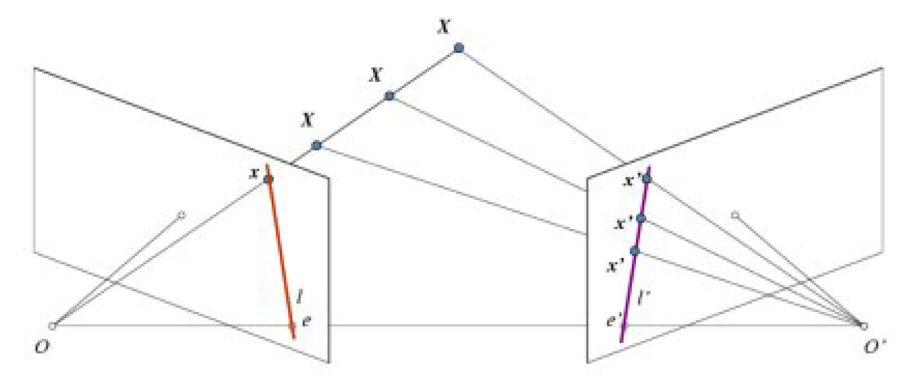
A complete camera model library for the PiCamera was implemented (Code 1, https://gitlab.etsit.urjc.es/jmvega/pibot-vision/tree/master/piCamModel). The camera model, assuming an ideal camera, is called the Pin-hole model. When an image is taken using a pin-hole camera, we lose important information, the depth of the image; i.e., how far each point in the image is from the camera, due to its 3D-to-2D conversion. Thus, an important question is how to find the depth information using cameras. One answer is to use more than one camera, as two cameras replicate the two eyes of humans, a concept known as stereo vision. Figure 11 shows a basic setup with two cameras taking an image from the same scene.

Code 1: PiCamera class.

As a single camera is used, the system cannot find the 3D point corresponding to pixel x in an image because every point on the line $OX$ projects to the same pixel on the image plane. Two cameras would capture two images and it would then be possible to triangulate the correct 3D point. In this case, to find the matching point in another image, it is unnecessary to search the whole image, being sufficient to search along the epiline. This is called Epipolar Constraint. Similarly, all points will have their corresponding epilines in the other image. Plane $XO{O}^{\prime }$ is called Epipolar Plane (see Figure 11). The intersections between Plane $XO{O}^{\prime }$ and the image planes form the epipolar lines.

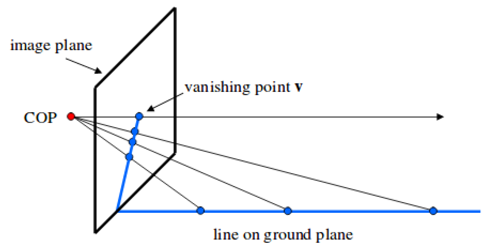
4.2.2. The Ground Hypothesis

To convey a depth map from the robot to the surrounding objects using a single camera, the ground hypothesis (Figure 12 is assumed. It considers all the objects are on the floor, on the ground plane, which is a known location (on plane $Z=0$). In this way, the 3D point corresponding to every point in the single image can be obtained (Figure 7).

Let us consider the pixels corresponding to the filtered border (Figure 7 right of the colored images) below the obstacles (Figure 7 left of the edged images), so that the distances can be calculated subsequently (Figure 7 bottom).

4.2.3. Coordinate Systems Transformations

To compute the rays back-projecting from the pixels and the rays projecting from 3D points into pixels, the position of the camera needs to be calculated (https://gitlab.etsit.urjc.es/jmvega/pibot-vision/blob/master/projGeomLibrary/projGeom.py). A camera is defined and positioned according to its matrices $K\ast R\ast T$ (

Table 1. Definition of pin-hole camera position parameters and orientation.

Camera Parameters	Definitions
K (3 × 3)	intrinsic parameters
R (3 × 3)	camera rotation
T (3 × 1)	camera translation
X	forward shift
Y	left shift
Z	upward shift

).

Instead of matrices R and T, a single matrix $RT(4\times 4)$ can be used, which includes $RT$, so would therefore be $4\times 4$, as shown in Equations (1)–(3), corresponding to rotation axes X, Y and Z.

$$\left[\begin{array}{cccc}1& 0& 0& X\\ 0& cos\left(\theta \right)& sin\left(\theta \right)& Y\\ 0& -sin\left(\theta \right)& cos\left(\theta \right)& Z\\ 0& 0& 0& 1\end{array}\right]$$

(1)

$$\left[\begin{array}{cccc}cos\left(\theta \right)& 0& -sin\left(\theta \right)& X\\ 0& 1& 0& Y\\ sin\left(\theta \right)& 0& cos\left(\theta \right)& Z\\ 0& 0& 0& 1\end{array}\right]$$

(2)

$$\left[\begin{array}{cccc}cos\left(\theta \right)& -sin\left(\theta \right)& 0& X\\ sin\left(\theta \right)& cos\left(\theta \right)& 0& Y\\ 0& 0& 1& Z\\ 0& 0& 0& 1\end{array}\right]$$

(3)

These three angles are used to build their three corresponding matrices, which are subsequently multiplied.

Let us consider an example using R and T matrices separately. Given a point in ground plane coordinates $P_g=[X,Y,Z]$, its coordinates in camera frame ($P_c$) are given by Equation (4).

$$P_c=R\times P_g+T$$

(4)

The camera center is $C_c=[0,0,0]$ in camera coordinates. Its ground coordinates are computed in Equation (5), where $R^{\prime }$ is the transpose of R and assuming, for simplicity, that the ground plane is $Z=0$.

$$C_g=-R^{\prime }\times T$$

(5)

Let K be the matrix of intrinsic parameters. Despite the intrinsic technical parameters being provided by the manufacturer (

Table 2. PiCamera (v2.1 board) technical intrinsic parameters.

PiCamera Parameters	Values
Sensor type	Sony IMX219PQ[7] CMOS 8-Mpx
Sensor size	3.674 × 2.760 mm (1/4${}^{″}$ format)
Pixel Count	3280 × 2464 (active pixels)
Pixel Size	1.12 × 1.12 um
Lens	f = 3.04 mm, f/2.0
Angle of View	62.2 × 48.8 degrees
SLR lens equivalent	29 mm

), the K values are more precisely obtained using the developed PiCamCalibrator (https://gitlab.etsit.urjc.es/jmvega/pibot-vision/tree/master/piCamCalibrator) tool. Given a pixel $q=[u,v]$, coordinates can be written in a homogeneous image as $Q=[u,v,1]$. Its location in camera coordinates ($Q_c$) is shown in Equation (6), where $K_i=inv\left(K\right)$ is the inverse of the intrinsic parameter matrix. The same point in world coordinates ($Q_g$) is given by Equation (7).

$$Q_c=K_i\times Q$$

(6)

$$Q_g=R^{\prime }\times Q_c-R^{\prime }\times t$$

(7)

All the points $Pg=[X,Y,Z]$ that belong to the ray going from the camera center through that pixel, expressed in ground coordinates, are then on the epipolar line given by Equation (8), where the $\theta$ value goes from 0 to positive infinity.

$$P_g=C_g+\theta \times (Q_g-C_g)$$

(8)

Due to the ground hypothesis being assumed (see Section 4.2.2), this epipolar line is intersected with ground plane (Code 2), where objects are assumed to be located.

Code 2: Intersection between optical ray and below border of object.

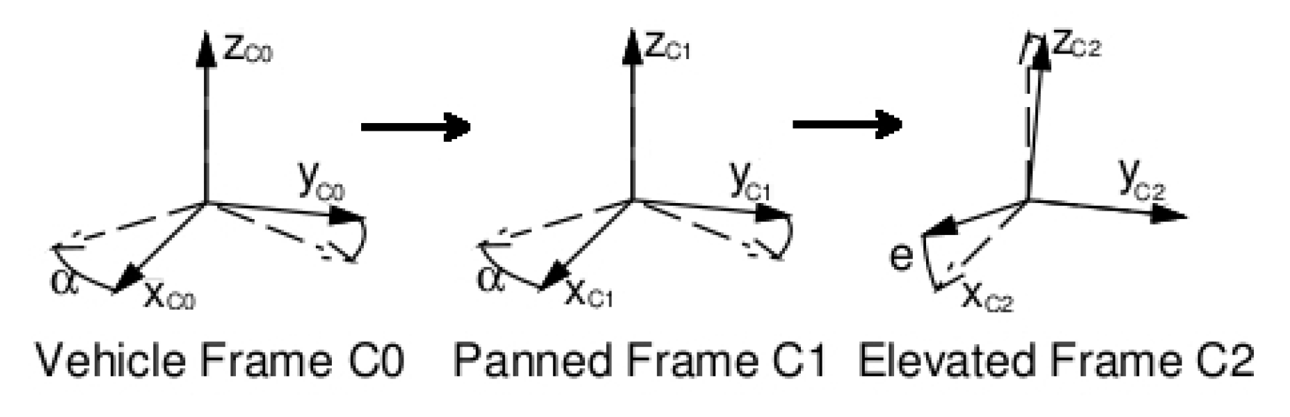
4.2.4. Camera Rotation and Translation

Every time the camera is moved with respect to several axes (as shown in Figure 13), camera matrices (Table 1) must be repeatedly multiplied. Thus, the following steps are needed for a complete translation of the camera:

• Considering robot encoders with information about X, Y and $\theta$, the robot is moved with respect to the absolute axis $(0,0)$ of the world, and rotated with respect to the Z axis, so the $RT$ matrix of the robot would be as shown in Equation (3).
• Assuming the camera is mounted over a Pan unit (servo), it is moved along the Z axis with respect to the base of the robot (which is on the ground level).
• Furthermore, the Pan axis is rotated with respect to the Z axis according to the Pan angle (Equation (3)).
• The Pan support is also rotated with respect to the Y axis according to the Tilt angle (Equation (2)), needed to perceive close objects.
• Finally, the optical center of the camera is translated in X and in Z with respect to the Tilt axis.

Thus, to obtain the absolute position of the camera in world coordinates, the five different matrices previously described are multiplied following Equation (9), and coded in Code 3.

$$\begin{array}{cc}\hfill & M_a=M_1\times M_2\hfill \\ \hfill & M_b=M_a\times M_3\hfill \\ \hfill & M_c=M_b\times M_4\hfill \\ \hfill & M_d=M_c\times M_5\hfill \end{array}$$

(9)

Code 3: Operations with camera matrices to get absolute position.

The absolute position $[X,Y,Z]$ of the camera is given by $M_d$, in cells $\left[\right[0,3],[1,3],[2,3\left]\right]$. The camera position and orientation can be expressed using $M_d$ and Focus of Attention (FOA). In this case, a column corresponding to the relative FOA $[X,Y,Z]$ is multiplied by the $M_d$ matrix resulting in an absolute FOA given by Equation (10).

$$FO{A}_{absolute}=M_d\times FO{A}_{relative}$$

(10)

4.3. Visual Attention Subsystem

In the previous section, we described in detail the operation of placing certain attributes in the robot’s visual memory. We will now describe the visual attention mechanism implemented (https://gitlab.etsit.urjc.es/jmvega/pibot-vision/tree/master/navAlgorithm).

The movement of the pan unit is properly controlled, directing the focus to three different positions. In our system, we considered all these three zones have the same preference of attention, so all of them are observed for the same time and with the same frequency. If different priorities were assigned to the zones, this would cause the pan unit to pose more times in one area than another.

When the look-sharing system chooses a focal point, it looks for a fixed time (0.5 s). For this monitoring, and to avoid excessive oscillations and have a more precise control over the pan unit, we decided to implement a P-controller to control the speed of the pan. This driver allows for command P or high speed, proportional to the pan-tilt unit, if the focus of attention to be targeted is far from the current position; or lower speeds if it requires small corrections.

The visual attention system presented here was implemented following a state-machine design, which determines when to execute the different steps of the algorithm. Thus, we can distinguish four states:

• Set next goal (State 0).
• Saccade movement is completed (State 1).
• Analyze image (State 2).
• Extract 3D edges (State 3).

Based on the initial state (or state 0), the system sets the next goal to be looked at and it then goes to State 1.

In State 1, the task is to complete the move towards the absolute position specified by State 0. Once there, the system goes to State 2, where the current image is analyzed.

Once the edge algorithm is finished, the system goes to State 3 and extracts the corresponding 3D edges, which are stored in the local memory. Finally, the system goes to State 0 and back again.

5. Experiments

The proposed system was evaluated using the real PiBot platform, with a Raspberry Pi 3B+ as main board (with Raspbian as operating system), and on which was mounted a Raspberry PiCamera v2.1 camera (described in Table 2) over a pan unit working in a pan range of [−80, 80] degrees. This pan was moved continuously using a Parallax Feedback 360deg high speed servo, which is able to work using PWM positional feedback across the entire angular range with a feedback-controllable rotation from −120 to 120 RPM.

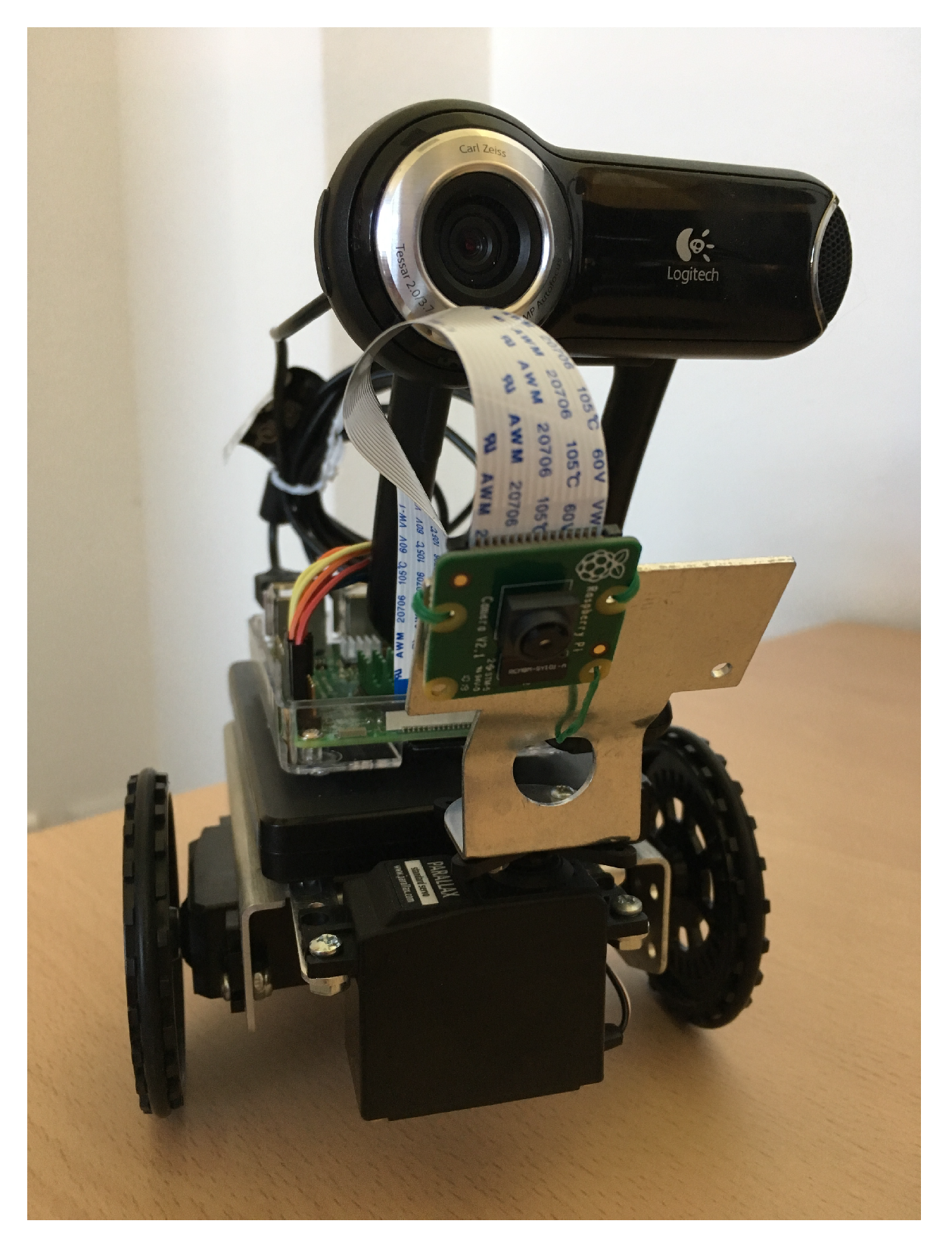
5.1. Performance Comparison: USB Webcam and CSI PiCamera

Since Raspberry Pi supports both common USB webcams and the PiCamera, through the CSI camera connector, the first experiment was conducted to verify and demonstrate whether the proposed system performance was improved using the camera module provided by Raspberry compared to a USB-connected camera (Figure 14).

The PiCamera used was the v2.1 model, (see Table 2), while the USB camera used was the Logitech QuickCam Pro 9000, whose features are described in

Table 3. Logitech QuickCam Pro 9000 technical specifications.

Logitech Camera Parameters	Values
Sensor type	Carl Zeiss (ICX098AK) CCD 2-Mpx
Sensor format	1/4″
Framerate	30 fps
Pixel Count	1600 × 1200 (active pixels)
Pixel Size	5.6 × 5.6 um
Lens	f = 2.96 mm, f/2.0
Plug	USB v2.0

.

Firstly, the definitions provided by both cameras were compared. The application used to capture images was fswebcam, chosen because of its simplicity, being a simple command-line app for Linux-based systems. Different resolutions were tested (1600 × 1200, 1280 × 960, 640 × 480) and the results were clear: the definition was much better in the PiCamera. Since it includes a 8 Mpx sensor compared to the 2 Mpx sensor of the Logitech camera, this result was expected. Although the Logitech camera yielded better results in poor lighting conditions, this was ignored, since the natural conditions in which our system will work is with good lighting conditions.

Secondly, the framerate was tested. A simple Python program was implemented for this comparison. Using the OpenCV videoCapture function and Time package to estimate times, we found that, setting the resolution to (320, 240), the Logitech ran on average at 14.97 fps and the PiCamera at 51.83 fps.

Finally, the edge detection algorithm (described in Section 4.1) was tested. It took 89 ms to obtain a complete visual sonar using either camera, since the algorithm does not depend on the vision sensor. However, according to the framerate results (and limited by processor computing capacity), to obtain a complete visual sonar, the proposed system took 108 ms using the PiCamera, compared to 169 ms taken by using the Logitech camera.

Summarizing, the PiCamera provides better performance than a webcam in terms of framerate and resolution, when running the visual system.

5.2. Distance Estimation Accuracy

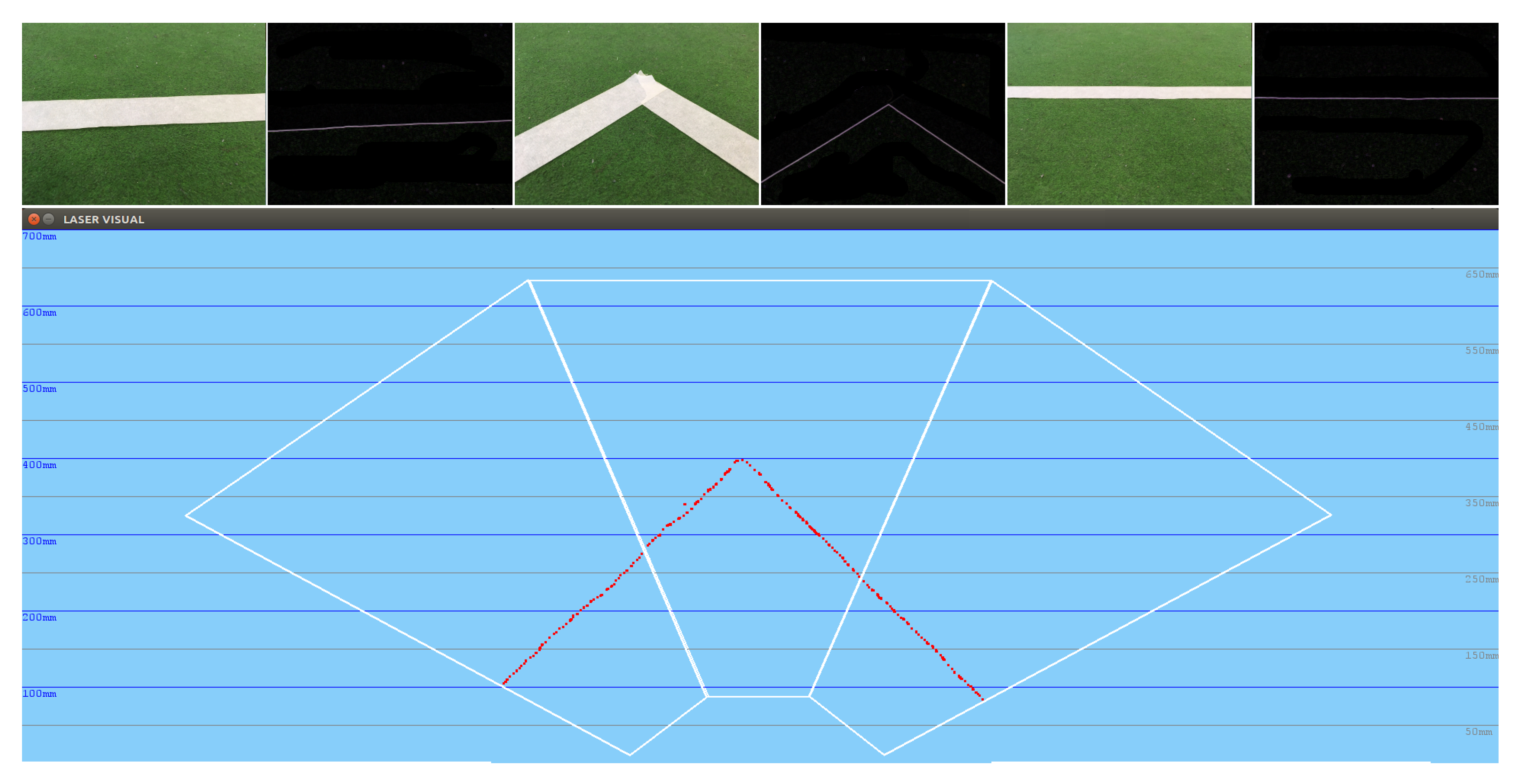
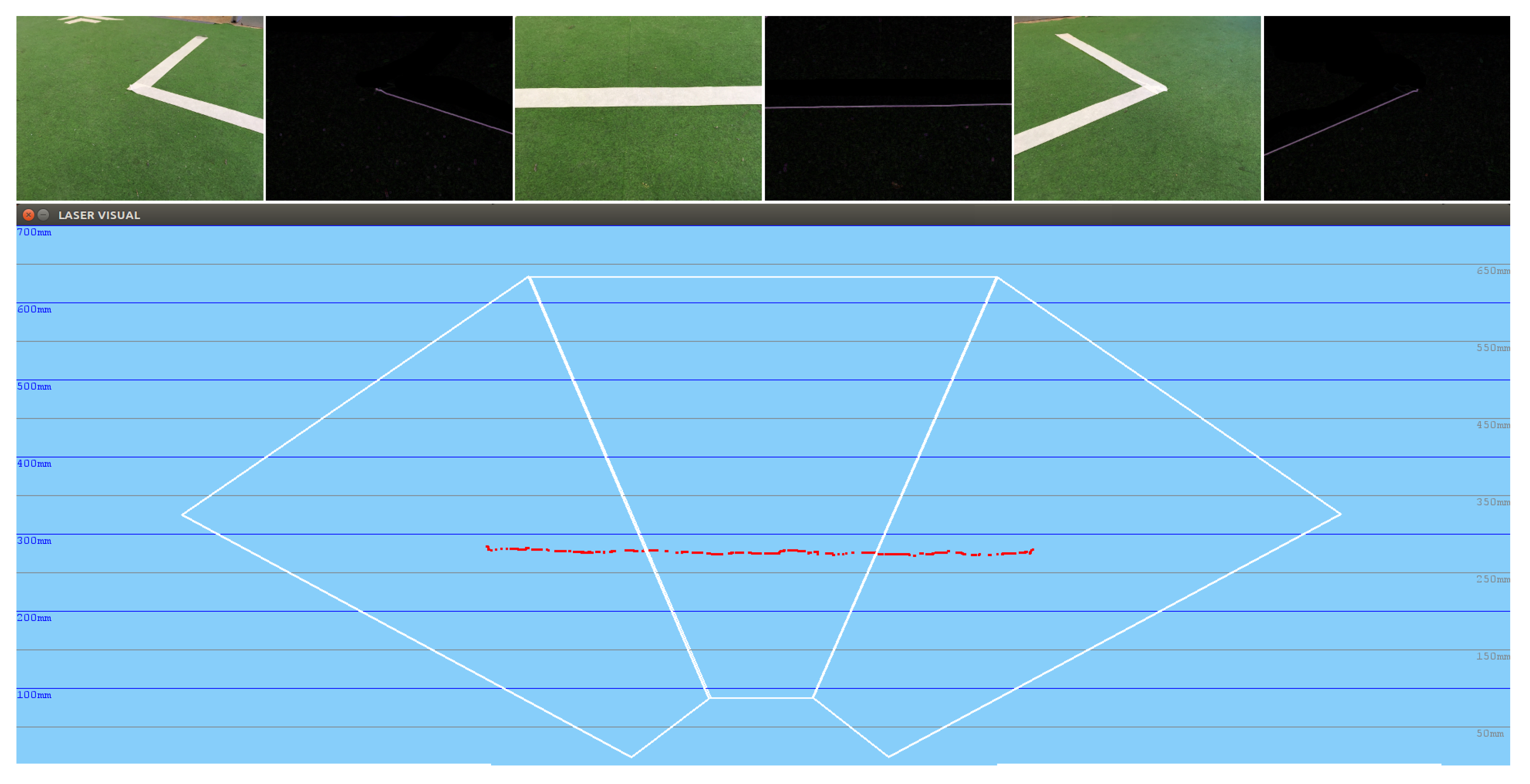
The distances obtained using the visual perception system described are feasible. Figure 15 shows how the system is able to obtain an exact straight 3D line, measured previously in reality. Moreover, thanks to the three-phase attentive system, it is able to see this complete line, which corresponds to the area of the soccer field used in the RoboCup.

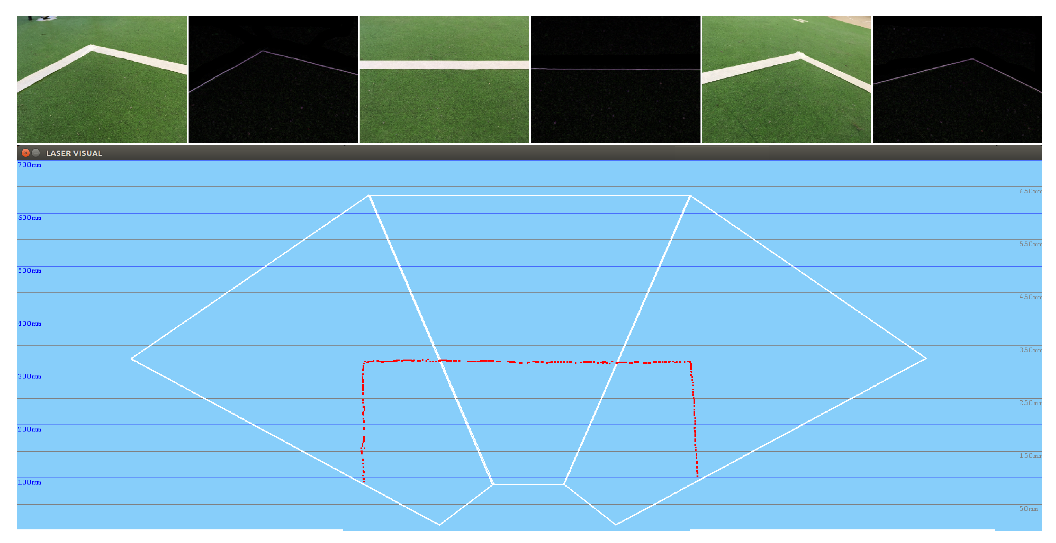
5.3. Educational Exercise: Navigation Using Visual Sonar

In the following experiment, the obstacle-avoidance navigation algorithm was tested, considering as obstacles the white lines on the ground, which mark the football field. In this case, far from presenting a clumsy behavior in which the robot headed towards the obstacles, as was the case when executing the same algorithm but with the ultrasonic sensor, the robot had greater obstacle memory and knew, in the situation shown in Figure 16, what was in the area between the corner and this area, and thus had no choice but to go back.

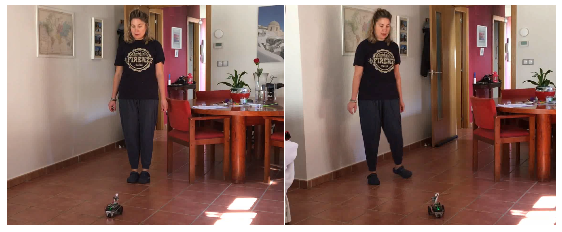
5.4. Educational Exercise: Navigation Following a Person

The object detector provided by the OpenCV library was used to detect a human face in the current image (Figure 17). The algorithm works internally with grayscale images and first requires training a cascade of Haar-type feature classifier stages, which are provided by a xml file.

Since this technique is computationally complex, and despite being optimized in OpenCV, several improvements had to be implemented because of the limited processor included in the Raspberry Pi. The main improvement was to ignore those regions of the image that reach a threshold of uniformity, since this implies that there will be no human face in them, considering that a human face is constantly in motion (Figure 18).

Starting from the detection of faces of the image perceived by the PiCamera, the camera field of vision was extended thanks to the mechanical neck that allows the camera to be moved. Thus, it was able to capture images even when the robot was stopped at a particular point.

6. Conclusions

This paper presents a visual system, the aim of which is to find obstacles around the robot and act accordingly. For this purpose, and thanks to a pan unit on which a camera is mounted, a visual attention mechanism was developed and tested on a real robotic platform under real circumstances.

The different experiments conducted show that the attention behaviors generated are quite similar to a human visual attention system. The detection algorithm presented is reasonably robust in different lighting conditions.

Moreover, since the scene is larger than the immediate field of view of the robot camera, a 3D visual short-term memory was implemented. The system continuously obtains basic information from the scene and incorporates it into a local short-term memory. This memory facilitates the internal representation of information around the robot, since obstacles may be placed in positions that the robot cannot see at a given time but knows their location.

As future research lines, deep learning techniques are being considered to recognize and consequently abstract the objects from the environment around the robot: basic shapes, traffic signals, human faces. In this way, the visual attention system could be adapted to steer the camera in order to detect the different visual elements and navigation signals, as well as potentially dangerous obstacles (such as walls). Once all the elements are detected, the system will incorporate them into its internal representation of the world, and will thus include them all in its gaze. This will let the robot navigate safely.

In line with the above, the intention is to use a new powerful board, whose hardware design is focused on improving the execution of computational vision algorithms. This new hardware is the Nvidia Jetson Nano, which is a Raspberry Pi-style hardware device with an embedded GPU and specifically designed to run deep learning models efficiently. Indeed, the Jetson Nano supports the exact same CUDA libraries for acceleration as those already used by almost every Python-based deep learning framework. Consequently, even existing Python-based deep learning algorithms could be run on the Jetson Nano with minimal modifications while a decent level of performance could still be achieved.