A Physical Layer Security Technique for NOMA Systems with MIMO SC-FDE Schemes

Abstract

Current wireless communication systems employ Multi-Input, Multi-Output (MIMO) techniques to increase spectral efficiency, at the cost of higher hardware complexity. Most of these systems continue to employ traditional Orthogonal Multiple Access (OMA) schemes, which are suboptimal when compared to Non-Orthogonal Multiple Access (NOMA) schemes. By combining NOMA with MIMO, it is possible to achieve higher spectral efficiencies. However, security in NOMA-MIMO systems remains a problem. In this paper, we study the physical layer security issues of a power based NOMA-MIMO system with a Singular Value Decomposition (SVD) scheme, employed along with Single Carrier with Frequency Domain Equalization (SC-FDE) techniques. We consider a scenario where there is an unintended eavesdropper attempting to listen to the messages being exchanged. It is shown that the higher the channel estimate correlation between transmitter and receiver, the higher the secrecy rate, particularly for a scenario where there is a Line-Of-Sight (LOS) between all users. Therefore, power based NOMA MIMO-SVD schemes, combined with SC-FDE, can be considered efficient options for highly secure MIMO communications.

1. Introduction

The increasing requirements for telecommunication systems have led to the research of Multiple-Input, Multiple-Output (MIMO) techniques, due to their large capacity gains over traditional single antenna system techniques [1]. In fact, these techniques have already been employed in recent standards, such as Wi-Fi [2] and LTE [3], and will be integrated in 5G systems [4].

In traditional Orthogonal Multiple Access (OMA) systems, radio resources are allocated to users in an orthogonal fashion (OFDMA, orthogonal CDMA, etc.), that is the uncoded messages meant for different users are never superimposed in the time and frequency domains. These systems, ideally, have no inter-user interference and require no additional processing for separating user’s at the receiver. However, due to new demands to further increase spectrum efficiency, Non-Orthogonal Multiple Access (NOMA) schemes are quickly surging as solutions due to their higher spectrum efficiency [5,6], even for mmWave systems [7]. In a NOMA scheme, two or more users’ messages are superimposed in the time and frequency domains, and user separation can be made in the power domain, leading to the so-called power domain NOMA [8]. It is also possible to allocate users among clusters [9]; however, in this work, we assume only two users, which can be approximated as a single cluster scenario [10]. The detection of the different users usually resorts to Successive Interference Cancellation (SIC) techniques.

Although there is a great benefit in adopting NOMA schemes, the security requirements are higher than the ones of traditional OMA schemes. This is explained by the fact that, when performing the SIC process, a user may decode messages meant for other users. Therefore, NOMA schemes can greatly benefit from Physical Layer Security (PLS) schemes [11,12,13,14], which can be combined with upper layer security techniques to ensure the confidentiality of a user’s message [15].

For this purpose, we chose to analyze the PLS characteristics of a Single Carrier (SC) NOMA-MIMO system employing Frequency Domain Equalization (FDE). Although there are many published works on PLS techniques, most of them focus on Orthogonal Frequency Division Multiplexing (OFDM) [16], and few are dedicated to SC systems. In [17], an SC system is analyzed, however, it does not consider a NOMA scenario, which poses additional security concerns. As is widely known, SC-FDE systems are appealing due to their lower Peak-to-Average Power Ratio (PAPR) when compared to multicarrier schemes. Moreover, when combined with non-linear iterative equalization techniques to mitigate Inter-Symbol Interference (ISI), such as Iterative Block-Decision Feedback Equalization (IB-DFE), they can achieve excellent performance, making this technique appealing for applications where there are strict energy efficiency requirements, as well as highly frequency selective channels. The security potential can be analyzed under various scenarios, such as in [18], where a friendly jammer and an eavesdropper were considered, or in [19], where a jammer and an eavesdropper worked together in an attempt to eavesdrop the system, or even through the use of artificial noise sequences at the transmitter [20]. This makes a direct comparison between these scenarios a challenging task. As such, in this work, we consider a simpler scenario with two independent eavesdroppers, which attempt to eavesdrop two different users.

In this work, we consider a novel Singular Value Decomposition (SVD) technique for separating user streams in MIMO-NOMA SC-FDE systems. More concretely, we analyze the security potential of this scheme in a scenario with an eavesdropper located near each user. Even in LOS scenarios, it is shown that the secrecy rate of the MIMO-NOMA system can be kept high if the multipath component’s power is relatively high.

This paper is organized as follows: In Section 2, we characterize the MIMO-NOMA system with its intended receivers, B and C, and eavesdropper E, with varying positions and targets. Section 3 concerns the system capacity and presents secrecy rate calculations. Section 4 shows the simulated Bit Error Rate (BER) and secrecy rate for all transmitter-receiver sets. Lastly, Section 5 concludes this paper.

2. Materials and Methods

2.1. System Characterization

In this paper, we consider a three user system, where one user, the transmitter A, attempts to communicate with the other two users, receivers B and C. The receivers are separated by a large distance, d, with one receiver, B, being close to the transmitter, while C is placed far from the transmitter. The transmitter employs a power based NOMA scheme and transmits both users’ signals at the same time. In addition, there is an eavesdropper near each user, attempting to listen to the messages being transmitted. A diagram summarizing this scenario can be seen in Figure 1. Although the transmitter’s position may vary, it is assumed that the distance to all other users is always much greater than the wavelength of the transmitted signal. The transmitter employs T antennas, while the receivers and eavesdropper employ R antennas. In order to handle the highly frequency selective channel, we employ an SC-FDE technique, combined with an appropriate Cyclic Prefix (CP) larger than the maximum overall channel impulse response.

The transmitter sends C data blocks, with $C\le R$, and each data block is composed by the sum of two blocks of N Quadrature Phase Shift Keying (QPSK) symbols with differing power (the generalization to other constellations is straightforward [21]). Contrary to the single user system studied in [17], fir the power domain NOMA scenario of this work, we must define the symbols to be transmitted to both users. The data symbols transmitted for user B are denoted by the $C\times N$ matrix ${\mathbf{s}}_B$, with each data stream defined as an $N\times 1$ vector ${\mathbf{s}}_B^{\left(c\right)}=[s_{1_B}^{\left(c\right)}{s}_{2_B}^{\left(c\right)}\cdots s_{N_B}^{\left(c\right)}]$. In that context, $s_{n_B}^{\left(c\right)}$ represents the QPSK symbol at the $n^{\mathrm{th}}$ time instant of the $c^{\mathrm{th}}$ data stream. The frequency domain counterpart of the data to be transmitted is denoted by ${\mathbf{S}}_B$. The group of symbols associated with the $k^{\mathrm{th}}$ subcarrier are defined as ${\mathbf{S}}_{k_B}=[S_{k_B}^{\left(1\right)}{S}_{k_B}^{\left(2\right)}..S_{k_B}^{\left(C\right)}]$. The symbols for User C are defined identically to the symbols for User B and denoted by ${\mathbf{s}}_C$, ${\mathbf{s}}_C^{\left(c\right)}$, ${\mathbf{S}}_C$, and ${\mathbf{S}}_{k_C}$, respectively. Under these conditions, the transmitted data at $n^{\mathrm{th}}$ time instant are defined as:

$${\mathbf{s}}_n={\mathbf{s}}_B+{\mathbf{s}}_C,$$

(1)

with a frequency domain counterpart defined as:

$${\mathbf{S}}_k={\mathbf{S}}_{k_B}+{\mathbf{S}}_{k_C}.$$

(2)

Since we are considering two receivers that are not co-located, we can define two channels, one from A to B and another from A to C. The frequency response for the $k^{\mathrm{th}}$ subcarrier of the channel from A to B is defined as:

$${\mathbf{H}}_{k_{AB}}=\left[\begin{array}{cccc}{H}_{k_{AB}}^{(1,1)}& H_{k_{AB}}^{(1,2)}& \cdots & H_{k_{AB}}^{(1,T)}\\ H_{k_{AB}}^{(2,1)}& H_{k_{AB}}^{(2,2)}& \cdots & H_{k_{AB}}^{(2,T)}\\ ⋮& ⋮& \ddots & ⋮\\ H_{k_{AB}}^{(R,1)}& H_{k_{AB}}^{(R,2)}& \cdots & H_{k_{AB}}^{(R,T)}\end{array}\right],$$

(3)

and the frequency response for the $k^{\mathrm{th}}$ subcarrier of the channel from A to C is defined as:

$${\mathbf{H}}_{k_{AC}}=\left[\begin{array}{cccc}{H}_{k_{AC}}^{(1,1)}& H_{k_{AC}}^{(1,2)}& \cdots & H_{k_{AC}}^{(1,T)}\\ H_{k_{AC}}^{(2,1)}& H_{k_{AC}}^{(2,2)}& \cdots & H_{k_{AC}}^{(2,T)}\\ ⋮& ⋮& \ddots & ⋮\\ H_{k_{AC}}^{(R,1)}& H_{k_{AC}}^{(R,2)}& \cdots & H_{k_{AC}}^{(R,T)}\end{array}\right].$$

(4)

In any MIMO system, the different channels must be separated, so as to avoid cross-channel interference. In this work, we employ a technique that combines precoding and decoding, which is based on the SVD in [22]. Calculating the SVD of the channel matrix requires Channel State Information (CSI) at both receivers and at the transmitter. This CSI can be obtained through the exchange of pilot sequences at the start of the transmission. In a Time Division Duplexing (TDD) system, this process is greatly simplified due to the reciprocity of the channel.

The SVD of each channel matrix is defined as:

$${\mathbf{H}}_{k_{AB}}={\mathbf{U}}_{k_{AB}}{\mathsf{\Lambda }}_{k_{AB}}{\mathbf{V}}_{k_{AB}}^H,$$

(5)

and:

$${\mathbf{H}}_{k_{AC}}={\mathbf{U}}_{k_{AC}}{\mathsf{\Lambda }}_{k_{AC}}{\mathbf{V}}_{k_{AC}}^H.$$

(6)

For simplicity’s sake, we omit the channel identifier (i.e., AB or AC) when we are referring to any channel. We denote ${\mathbf{U}}_k$ as the $R\times R$ decoding matrix, ${\mathbf{V}}_k$ as the $T\times T$ precoding matrix, and ${\mathsf{\Lambda }}_k$ as an $C\times C$ diagonal matrix composed by the singular values of ${\mathbf{H}}_k$, which are sorted in descending order according to their power.

2.2. Transmission

In a power domain NOMA scheme, the data meant for each user are sent at the same time and over the same channel, with differing transmitting power. In this work, we define the ratio between the power of ${\mathbf{S}}_{k_B}$ and ${\mathbf{S}}_{k_C}$ as $\alpha$.

It is widely known that the performance of a given stream in an SVD system depends on the singular value power of that stream. A simple scheme for averaging the performance of all streams was proposed in [23], which consisted of interleaving the data symbols before applying the precoding technique. The interleaving scheme can be different for each user, as it only affects the data symbols. Therefore, we define the interleaved symbols for Users B and C as ${\mathbf{S}}_{k_B}^{{}^{\prime }}$ and ${\mathbf{S}}_{k_C}^{{}^{\prime }}$, respectively.

Before transmitting data, there is an initial training sequence exchange between all users, so as to obtain the channel matrices with which to compute the SVD. The exchange begins with the farthest user, C, sending a training sequence meant for the transmitter, which is ignored by B. In the next step, B sends a training sequence meant for the transmitter as well. Lastly, the transmitter sends a training sequence, followed by the precoded data to all users. In all steps, there is an eavesdropper that listens to all of the exchanged sequences and computes its own channel estimates.

As described in [24], the channel matrices associated with the $k^{\mathrm{th}}$ subcarrier can be defined as:

$${\mathbf{H}}_{k_{AB}}={\rho }_{A1}{\widehat{\mathbf{H}}}_{k_{A1}}+{\mathit{ϵ}}_k,$$

(7)

and:

$${\mathbf{H}}_{k_{AC}}={\rho }_{A2}{\widehat{\mathbf{H}}}_{k_{A2}}+{\mathit{ϵ}}_k,$$

(8)

where ${\widehat{\mathbf{H}}}_{k_{A}1}$ and ${\widehat{\mathbf{H}}}_{k_{A}2}$ are the channel estimates used by the transmitter, ${\rho }_{A1}$ and ${\rho }_{A2}$ are correlation factors with the true channels, and ${\mathit{ϵ}}_k$ is the error associated with the channel estimation process (our analysis can be easily extended to other models for the channel estimation errors). This error ${\mathit{ϵ}}_k$ is characterized as a complex variable with a Gaussian distribution and variance $2{\sigma }_N^2/\beta$, where ${\sigma }_N^2$ is the noise variance for a specific Signal-to-Noise Ratio (SNR) value and $\beta$ is a scaling factor. For $\beta \to \infty$ and ${\rho }_{A1}={\rho }_{A2}=1$, there is a perfect channel estimation, i.e., ${\widehat{\mathbf{H}}}_{k_{AB}}={\mathbf{H}}_{k_{A1}}$ and ${\widehat{\mathbf{H}}}_{k_{AC}}={\mathbf{H}}_{k_{A2}}$. We define the SVD of the channel estimates as:

$${\widehat{\mathbf{H}}}_{k_{A1}}={\widehat{\mathbf{U}}}_{k_{A1}}{\widehat{\mathsf{\Lambda }}}_{k_{A1}}{\widehat{\mathbf{V}}}_{k_{A1}}^H,$$

(9)

and:

$${\widehat{\mathbf{H}}}_{k_{A2}}={\widehat{\mathbf{U}}}_{k_{A2}}{\widehat{\mathsf{\Lambda }}}_{k_{A2}}{\widehat{\mathbf{V}}}_{k_{A2}}^H.$$

(10)

Using the result of SVD, the transmitter performs the precoding operation defined as:

$${\mathbf{X}}_k={\widehat{\mathbf{V}}}_{k_{A}1}{\mathbf{S}}_{k_B}^{\prime }+\sqrt{\alpha }{\widehat{\mathbf{V}}}_{k_{A}1}{\mathbf{S}}_{k_C}^{\prime },$$

(11)

where ${\mathbf{X}}_k$ is the signal to be transmitted and $\alpha$ is the ratio between the power transmitted meant for User C and the power transmitted meant for User B. Since the precoding operation only utilizes the channel estimate of the close user, additional information must be sent to allow the far user to complete the SVD process. The transmitter sends a partial key ${\mathbf{Q}}_k$, which is defined as:

$${\mathbf{Q}}_k={\widehat{\mathbf{V}}}_{k_{A}1}^H{\widehat{\mathbf{V}}}_{k_{A}2}.$$

(12)

Since ${\mathbf{Q}}_k$ is a unitary matrix, then for the case of a system with $T=R=2$, this matrix can be written as:

$${\mathbf{Q}}_k=\left[\begin{array}{cc}a& b\\ -b^{\ast }exp\left(j\varphi \right)& a^{\ast }exp\left(j\varphi \right)\end{array}\right],$$

(13)

where a and b are complex coefficients such that ${\left|a\right|}^2+{\left|b\right|}^2=1$, and the determinant of this matrix is given by:

$$det\left({\mathbf{Q}}_k\right)=exp\left(j\varphi \right).$$

(14)

Under this decomposition, the transmitter must send four parameters that allow for the reconstruction of the original matrix. These parameters are $\left|a\right|$, $arg\left(a\right)$, $arg\left(b\right)$, and $det\left({\mathbf{Q}}_k\right)$, which are all real valued quantities that can be quantized with a low resolution, so as to reduce the overhead associated with the transmission of the partial key.

2.3. Reception

The received signal at User B can be defined as:

$${\mathbf{Z}}_{k_B}={\mathbf{H}}_{k_{AB}}{\mathbf{X}}_k+{\mathbf{N}}_k,$$

(15)

while the received signal at User C is defined as:

$${\mathbf{Z}}_{k_C}={\mathbf{H}}_{k_{AC}}{\mathbf{X}}_k+{\mathbf{N}}_k.$$

(16)

Before decoding the symbols, both receivers employ the Iterative Block-Decision Feedback Equalization (IB-DFE) technique [25] with soft decisions. This technique utilizes feedback from the soft decided symbols to improve the equalization and mitigate the intersymbol interference in frequency selective channels. Figure 2 shows a simplified diagram of this system. However, it should be noted that this 2userscheme must be slightly changed for our power domain NOMA scenario, mainly due to the SIC and partial key requirements at each receiver.

2.4. Receiver B

As described earlier, User B also computes a channel estimation, with the training sequence transmitted by A. We can express the channel as:

$$H_{k_{AB}}={\rho }_B{\widehat{\mathbf{H}}}_{k_B}+{\mathit{ϵ}}_k,$$

(17)

where ${\rho }_B$ is a correlation factor with the true channel. It is not unreasonable to assume that there is a high correlation between the estimate of the receiver B and the transmitter; therefore, we can assume ${\rho }_{A1}={\rho }_B\approx 1$. For simplicity, we assume that the error distribution of the channel estimate is the same for both A and B, though the generalization to other cases is straightforward. The SVD of the channel estimate at User B is written as:

$${\widehat{\mathbf{H}}}_{k_B}={\widehat{\mathbf{U}}}_{k_B}{\widehat{\mathsf{\Lambda }}}_{k_B}{\widehat{\mathbf{V}}}_{k_B}^H,$$

(18)

with ${\widehat{\mathbf{U}}}_{k_B}$, ${\widehat{\mathsf{\Lambda }}}_{k_B}$, and ${\widehat{\mathbf{V}}}_{k_B}^H$ being the corresponding estimates of the matrices defined in (5).

As in conventional SVD techniques, the decoding is performed by multiplying the signal by the decoding matrix ${\widehat{\mathbf{U}}}_{k_B}$, which is computed as:

$${\mathbf{W}}_{k_B}^{\prime }={\widehat{\mathbf{U}}}_{k_B}^H{\mathbf{Z}}_{k_B},$$

(19)

where ${\mathbf{W}}_{k_B}^{\prime }$ is a $C\times 1$ column vector with the interleaved, decoded symbols. This operation can be expanded as:

$$\begin{array}{cc}\hfill {\mathbf{W}}_{k_B}^{\prime }& ={\widehat{\mathbf{U}}}_{k_B}^H{\mathbf{H}}_{k_{AB}}{\mathbf{X}}_k+{\widehat{\mathbf{U}}}_{k_B}^H{\mathbf{N}}_k\hfill \\ \hfill & ={\widehat{\mathbf{U}}}_{k_B}^H{\mathbf{H}}_{k_{AB}}{\mathbf{V}}_{k_{A1}}({\mathbf{S}}_{k_B}^{\prime }+\sqrt{\alpha }{\mathbf{S}}_{k_C}^{\prime })+{\widehat{\mathbf{U}}}_{k_B}^H{\mathbf{N}}_k\hfill \\ \hfill & ={\widehat{\mathsf{\Lambda }}}_{k_{AB}}({\mathbf{S}}_{k_B}^{\prime }+\sqrt{\alpha }{\mathbf{S}}_{k_C}^{\prime })+{\widehat{\mathbf{U}}}_{k_B}^H{\mathbf{N}}_k,\hfill \end{array}$$

(20)

with ${\widehat{\mathsf{\Lambda }}}_{k_{AB}}$ corresponding to an estimate of the diagonal matrix composed by the singular values of the channel. Before performing equalization, however, the receiver must perform deinterleaving, to restore the original symbol order, yielding:

$${\mathbf{W}}_{k_B}={\widehat{\mathsf{\Lambda }}}_{k_{AB}}^{\prime }({\mathbf{S}}_{k_B}+\sqrt{\alpha }{\mathbf{S}}_{k_C})+{\widehat{\mathbf{U}}}_{k_B}^{\prime H}{\mathbf{N}}_k^{\prime }.$$

(21)

After the deinterleaving, each stream is affected by a frequency selective channel made up of the different singular values.

Before User B can detect its intended symbols, it must perform the SIC reception on the symbols intended for User C. In order to do so, it first performs detection on the stronger signal, which has a much higher Signal-to-Noise Ratio (SNR) than the wanted signal, making the detection simple.

The equalized signal is obtained by computing:

$${\tilde{\mathbf{S}}}_{k_C}={\mathbf{F}}_{k_{B1}}{\mathbf{W}}_{k_B},$$

(22)

where the equalization factor ${\mathbf{F}}_{k_{B1}}$ is defined according to Minimum Mean Squared Error (MMSE) criterion as:

$${\mathbf{F}}_{k_{B1}}=\frac{{\widehat{\mathsf{\Lambda }}}_{k_B}^{{}^{\prime }}}{{\widehat{\mathsf{\Lambda }}}_{k_B}^{{}^{\prime }2}+\frac{1}{\sqrt{\alpha }\mathrm{SNR}}}.$$

(23)

Subsequently, the receiver computes hard decisions of the transmitted symbols as:

$${\widehat{\mathbf{S}}}_{k_C}=sign\left(\mathrm{Re}\left({\tilde{\mathbf{S}}}_{k_C}\right)\right)+jsign\left(\mathrm{Im}\left({\tilde{\mathbf{S}}}_{k_C}\right)\right),$$

(24)

with ${\widehat{\mathbf{S}}}_{k_C}$ being a hard decided estimate of the transmitted symbols meant for User C. Using this estimate, the receiver can perform detection on the intended symbols.

In the scenario where there is a nearby eavesdropper, E, attempting to listen to the message being sent to B, then it must attempt to estimate the channel between A and B. Since an eavesdropper cannot attempt to estimate this channel, it estimates two different channels, defined as:

$${\mathbf{H}}_{k_{EB1}}={\rho }_{EB1}{\widehat{\mathbf{H}}}_{k_{EB1}}+{\xi }_k+{\mathit{ϵ}}_k$$

(25)

and:

$${\mathbf{H}}_{k_{EB2}}={\rho }_{EB2}{\widehat{\mathbf{H}}}_{k_{EB2}}+{\xi }_k+{\mathit{ϵ}}_k,$$

(26)

where ${\mathbf{H}}_{k_{EB1}}$ is the channel between A and E, ${\mathbf{H}}_{k_{EB2}}$ is the channel between B and E, ${\rho }_{EB1}$ and ${\rho }_{EB2}$ are correlation coefficients with the true channels, and ${\xi }_k$ is an appropriate Gaussian distributed error term with variance ${\sigma }_N^2/{\beta }_M$, where ${\beta }_M$ is a scaling factor. Since the eavesdropper does not know the channel, we can assume that ${\rho }_{EB1}={\rho }_{EB2}<1$. For simplicity’s sake, we assume that ${\rho }_{EB1}={\rho }_{EB2}={\rho }_{EB}$. In order to increase the accuracy of the channel estimate, the receiver can compute the average of both intermediate channels, i.e.,

$${\mathbf{H}}_{k_{AB}}=\frac{{\mathbf{H}}_{k_{EB1}}+{\mathbf{H}}_{k_{EB2}}}{2}.$$

(27)

Iterative Equalization

To reduce the ISI, the receiver and eavesdropper employ an iterative frequency domain equalization scheme based on the IB-DFE [25] and MMSE criterion, which performs both feedforward and feedback equalization at a subcarrier level. This equalization process can be repeated up to L times, which we fixed at $L=4$ for this work.

The equalized symbols at the $k^{\mathrm{th}}$ subcarrier and $l^{\mathrm{th}}$ iteration are computed by:

$${\tilde{\mathbf{S}}}_{k_B}^{\left(l\right)}={\mathbf{F}}_{k_{B2}}^{\left(l\right)}\left({\mathbf{W}}_{k_B}-\sqrt{\alpha }{\widehat{\mathsf{\Lambda }}}_{k_B}^{{}^{\prime }}{\widehat{\mathbf{S}}}_{k_C}\right)-{\mathbf{B}}_{k_{B2}}^{\left(l\right)}{\overline{\mathbf{S}}}_{k_B}^{(l-1)},$$

(28)

where ${\mathbf{F}}_{k_{B2}}^{\left(l\right)}$ is the feedforward factor, ${\mathbf{B}}_{k_{B2}}^{\left(l\right)}$ is the feedback factor, and ${\overline{\mathbf{S}}}_{k_B}^{(l-1)}$ are the soft decided symbols of the previous iteration (for $l=1$, this is simply a null vector). The feedforward factor matrix is defined as:

$${\mathbf{F}}_{k_{B2}}^{\left(l\right)}=\frac{{\widehat{\mathsf{\Lambda }}}_{k_B}^{{}^{\prime }}}{\left(1-{\left|{\rho }^{(l-1)}\right|}^2\right){\widehat{\mathsf{\Lambda }}}_{k_B}^{{}^{\prime }2}+\frac{1}{\mathrm{SNR}}},$$

(29)

where ${\rho }^{(l-1)}$ denotes the block-wise reliability associated with the data estimated in the ${(l-1)}^{\mathrm{th}}$ iteration (when $l=1$, we have ${\rho }^{\left(0\right)}=0$). The feedback factor matrix, on the other hand, is defined as:

$${\mathbf{B}}_{k_B}^{\left(l\right)}={\mathbf{F}}_{k_{B2}}^{\left(l\right)}{\widehat{\mathsf{\Lambda }}}_{k_B}^{{}^{\prime }}-\mathbf{I}.$$

(30)

2.5. Receiver C

The detection at User C is significantly different from the detection scheme employed in [17]. This is explained by the modifications required for the interleaving scheme and by the use of a partial key. As described earlier, User C also computes a channel estimation, with the training sequence transmitted by A. We can express the channel as:

$$H_{k_{AC}}={\rho }_C{\widehat{\mathbf{H}}}_{k_C}+{\mathit{ϵ}}_k.$$

(31)

where ${\rho }_C$ is a correlation factor with the true channel. It is not unreasonable to assume that there is a high correlation between the estimate of the receiver C and the transmitter; therefore, we can assume ${\rho }_{A2}={\rho }_C\approx 1$. For simplicity, we assume that the error distribution of the channel estimate is the same for both A and C, though the generalization to other cases is straightforward. The SVD of the channel estimate at User C is written as:

$${\widehat{\mathbf{H}}}_{k_C}={\widehat{\mathbf{U}}}_{k_C}{\widehat{\mathsf{\Lambda }}}_{k_C}{\widehat{\mathbf{V}}}_{k_C}^H,$$

(32)

with ${\widehat{\mathbf{U}}}_{k_C}$, ${\widehat{\mathsf{\Lambda }}}_{k_C}$ and ${\widehat{\mathbf{V}}}_{k_C}^H$ being the corresponding estimates of the matrices defined in (6).

As in conventional SVD techniques, the decoding is performed by multiplying the signal by the decoding matrix ${\widehat{\mathbf{U}}}_{k_C}$, which is computed as:

$${\mathbf{W}}_{k_C}^{\prime }={\widehat{\mathbf{U}}}_{k_C}^H{\mathbf{Z}}_{k_C},$$

(33)

where ${\mathbf{W}}_{k_C}^{\prime }$ is a $C\times 1$ column vector with the interleaved, decoded symbols. This operation can be expanded as:

$$\begin{array}{cc}\hfill {\mathbf{W}}_{k_C}^{\prime }& ={\widehat{\mathbf{U}}}_{k_B}^H{\mathbf{H}}_{k_{AC}}{\mathbf{X}}_k+{\widehat{\mathbf{U}}}_{k_C}^H{\mathbf{N}}_k\hfill \\ \hfill & ={\widehat{\mathbf{U}}}_{k_C}^H{\mathbf{H}}_{k_{AC}}{\mathbf{V}}_{k_{A1}}({\mathbf{S}}_{k_B}^{\prime }+\sqrt{\alpha }{\mathbf{S}}_{k_C}^{\prime })+{\widehat{\mathbf{U}}}_{k_C}^H{\mathbf{N}}_k\hfill \\ \hfill & ={\widehat{\mathsf{\Lambda }}}_{k_{AC}}{\mathbf{V}}_{k_C}^H{\mathbf{V}}_{k_{A1}}({\mathbf{S}}_{k_B}^{\prime }+\sqrt{\alpha }{\mathbf{S}}_{k_C}^{\prime })+{\widehat{\mathbf{U}}}_{k_C}^H{\mathbf{N}}_k,\hfill \end{array}$$

(34)

with ${\widehat{\mathsf{\Lambda }}}_{k_{AC}}$ corresponding to an estimate of the diagonal matrix composed by the singular values of the channel. The received signal is then deinterleaved, so as to split the singular values amongst the streams, yielding:

$${\mathbf{W}}_{k_C}={\widehat{\mathsf{\Lambda }}}_{k_{AC}}^{\prime }{\mathbf{V}}_{k_C}^{\prime H}{\mathbf{V}}_{k_{A1}}^{\prime }({\mathbf{S}}_{k_B}+\sqrt{\alpha }{\mathbf{S}}_{k_C})+{\widehat{\mathbf{U}}}_{k_C}^{\prime H}{\mathbf{N}}_k^{\prime }.$$

(35)

As was the case with Receiver B, this receiver performs the same iterative equalization, with the exception that it does not need to perform an initial first detection. The equalization is defined as:

$${\mathbf{Y}}_{k_C}^{\left(l\right)}={\mathbf{F}}_{k_C}^{\left(l\right)}{\mathbf{W}}_{k_C}-{\mathbf{B}}_{k_C}^{\left(l\right)}{\overline{\mathbf{Y}}}_{k_C}^{(l-1)},$$

(36)

where ${\mathbf{Y}}_{k_C}^{\left(l\right)}$ is the equalized received signal at the $k^{\mathrm{th}}$ subcarrier and $l^{\mathrm{th}}$ iteration and ${\overline{\mathbf{Y}}}_{k_C}^{(l-1)}$ is the equalized signal estimate of the previous iteration (for $l=1$, it is set to 0). However, unlike Receiver B, this receiver cannot complete the SVD on its own. Therefore, it makes use of the partial key ${\widehat{\mathbf{Q}}}_k$, which is computed from the received parameters as:

$${\mathbf{Q}}_k=\left[\begin{array}{cc}\tilde{a}expj{\tilde{\varphi }}_a& \tilde{b}expj{\tilde{\varphi }}_b\\ -\tilde{b}expj(\tilde{\varphi }-{\tilde{\varphi }}_b)& \tilde{a}expj(\tilde{\varphi }-{\tilde{\varphi }}_a)\end{array}\right],$$

(37)

where $\tilde{a}$,${\tilde{\varphi }}_a$, ${\tilde{\varphi }}_b$, and $\tilde{\varphi }$ are the finite resolution quantized values transmitted by A and $\tilde{b}$ is obtained from $\tilde{b}=\sqrt{1-{\tilde{a}}^2}$. Prior to applying the partial key, the equalized signal is interleaved, in order to match the SVD matrices. The equalized symbols estimates are expressed as:

$${\tilde{\mathbf{S}}}_{k_C}^{\prime \left(l\right)}={\mathbf{Q}}_k{\mathbf{Y}}_{k_C}^{\prime \left(l\right)},$$

(38)

which are then deinterleaved into the equalized symbol estimates ${\tilde{\mathbf{S}}}_{k_C}^{\left(l\right)}$.

In the scenario where there is a nearby eavesdropper, E, attempting to listen to the message being sent to C, then it must attempt to estimate the channel between A and C. Since an eavesdropper cannot attempt to estimate this channel, it estimates two different channels, defined as:

$${\mathbf{H}}_{k_{EC1}}={\rho }_{EC1}{\widehat{\mathbf{H}}}_{k_{EC1}}+{\xi }_k+{\mathit{ϵ}}_k$$

(39)

and:

$${\mathbf{H}}_{k_{EC2}}={\rho }_{EC2}{\widehat{\mathbf{H}}}_{k_{EC2}}+{\xi }_k+{\mathit{ϵ}}_k,$$

(40)

where ${\mathbf{H}}_{k_{EC1}}$ is the channel between A and E, ${\mathbf{H}}_{k_{EC2}}$ is the channel between B and E, and ${\rho }_{EC1}$ and ${\rho }_{EC2}$ are correlation coefficients with the true channels. Since the eavesdropper does not know the channel, we can assume that ${\rho }_{EC1}={\rho }_{EC2}<1$. Once again, for simplicity’s sake, we assume that ${\rho }_{EC1}={\rho }_{EC2}={\rho }_{EC}$. In order to increase the accuracy of the channel estimate, the receiver can compute the average of both intermediate channels, i.e.,

$${\mathbf{H}}_{k_{AC}}=\frac{{\mathbf{H}}_{k_{EC1}}+{\mathbf{H}}_{k_{EC2}}}{2}.$$

(41)

2.6. Line-of-Sight Link Scenario

An additional scenario where there is LOS between the transmitter and all other users can be considered. In these conditions, the channel is defined as the sum of an LOS component (without fading effects) and several multipath rays (which are uncorrelated and have fading). In the worst case scenario, the eavesdropper can estimate the LOS component, albeit with a certain error; however, that is not feasible for the remaining multipath rays [26]. In this case, we define the channels as:

$${\mathbf{H}}_{k_{AB},los}={\mathbf{D}}_{k_{AB},los}+{\mathbf{R}}_{k_{AB},mp},$$

(42)

and:

$${\mathbf{H}}_{k_{AC},los}={\mathbf{D}}_{k_{AC},los}+{\mathbf{R}}_{k_{AC},mp},$$

(43)

where ${\mathbf{D}}_{k_{AB},los}$ and ${\mathbf{D}}_{k_{AC},los}$ are the low fading, highly correlated LOS components and ${\mathbf{R}}_{k_{AB},mp}$ and ${\mathbf{R}}_{k_{AC},mp}$ are the high fading multipath components of the respective channels. We then substitute these channels in (7), (8), (17), and (31) as:

$${\mathbf{H}}_{k_{AB},los}={\rho }_{A1}{\widehat{\mathbf{H}}}_{k_{A1},los}+{\mathit{ϵ}}_k,$$

(44)

$${\mathbf{H}}_{k_{AC},los}={\rho }_{A2}{\widehat{\mathbf{H}}}_{k_{A2},los}+{\mathit{ϵ}}_k,$$

(45)

$${\mathbf{H}}_{k_{AB},los}={\rho }_B{\widehat{\mathbf{H}}}_{k_B,los}+{\mathit{ϵ}}_k,$$

(46)

$${\mathbf{H}}_{k_{AC},los}={\rho }_C{\widehat{\mathbf{H}}}_{k_C,los}+{\mathit{ϵ}}_k.$$

(47)

The receivers’ and transmitter’s remaining operations are calculated as described previously.

The eavesdropper, however, cannot estimate the multipath component of the channel and must instead rely on the estimate of the LOS component. We define this component for the eavesdropper estimating the closest user as:

$${\mathbf{D}}_{k_{AB},los}=\frac{{\mathbf{H}}_{k_{EB1,los}}+{\mathbf{H}}_{k_{EB2,los}}}{2},$$

(48)

where:

$${\mathbf{H}}_{k_{EB1,los}}={\rho }_{EB1}{\widehat{\mathbf{H}}}_{k_{EB1,los}}+{\xi }_k+{\mathit{ϵ}}_k$$

(49)

and:

$${\mathbf{H}}_{k_{EB2,los}}={\rho }_{EB2}{\widehat{\mathbf{H}}}_{k_{EB2,los}}+{\xi }_k+{\mathit{ϵ}}_k.$$

(50)

Likewise, the component for the eavesdropper estimating the farthest user is defined as:

$${\mathbf{D}}_{k_{AC},los}=\frac{{\mathbf{H}}_{k_{EC1,los}}+{\mathbf{H}}_{k_{EC2,los}}}{2},$$

(51)

where:

$${\mathbf{H}}_{k_{EC1,los}}={\rho }_{EC1}{\widehat{\mathbf{H}}}_{k_{EC1,los}}+{\xi }_k+{\mathit{ϵ}}_k$$

(52)

and:

$${\mathbf{H}}_{k_{EC2,los}}={\rho }_{EC2}{\widehat{\mathbf{H}}}_{k_{EC2,los}}+{\xi }_k+{\mathit{ϵ}}_k.$$

(53)

In this scenario, the channel estimates ${\widehat{\mathbf{H}}}_{k_{EB1,los}}$ and ${\widehat{\mathbf{H}}}_{k_{EB2,los}}$, likewise with the channel estimates ${\widehat{\mathbf{H}}}_{k_{EC1,los}}$ and ${\widehat{\mathbf{H}}}_{k_{EC2,los}}$, only concern the LOS component between A and E and B and E or between A and E, and A and C, respectively. The difference between these estimates and the real channels will be proportional to the power of the multipath component. We define the ray power coefficient for both scenarios as:

$${\alpha }_{RP}=\frac{P_R}{P_D+P_R},$$

(54)

where $P_D$ and $P_R$ are the powers of the LOS and multipath components, respectively. Clearly, if ${\alpha }_{RP}=0$, the channel is only composed by the LOS component, whereas at ${\alpha }_{RP}=1$, the channel is composed of only the multipath component.

2.7. Decision Feedback

The definitions in this section, unless otherwise stated, apply to all receivers. As is known, employing soft decisions in the feedback equalization greatly reduces the level of ISI. These soft decisions can be calculated through the log likelihood ratios (LLR) of the equalized signal, obtained by:

$$L_n^{(\mathrm{I},i)}=\frac{2}{{\sigma }_i^2}\mathrm{Re}\left({\tilde{s}}_n^{\left(i\right)}\right),$$

(55)

and:

$$L_n^{(\mathrm{Q},i)}=\frac{2}{{\sigma }_i^2}\mathrm{Im}\left({\tilde{s}}_n^{\left(i\right)}\right),$$

(56)

where:

$${\sigma }_i^2=\frac{1}{2}\mathbb{E}\left[{\left|s_n-{\tilde{s}}_n^{\left(i\right)}\right|}^2\right]\approx \frac{1}{2N}\sum _{n=0}^{N-1}{\left|{\widehat{s}}_n-{\tilde{s}}_n^{\left(i\right)}\right|}^2.$$

(57)

After obtaining the LLR for each bit, we can calculate the soft decision of a given data symbol as:

$${\overline{s}}_n^{\left(i\right)}=tanh\left(\frac{L_n^{(\mathrm{I},i)}}{2}\right)+jtanh\left(\frac{L_n^{(\mathrm{Q},i)}}{2}\right).$$

(58)

The estimated data symbols are obtained through the hard decision of the equalized symbols. For Receiver C, there is an additional step, which consists of, once again, interleaving the soft decided symbols and multiplying by the Hermitian of the partial key matrix, written as:

$${\overline{\mathbf{Y}}}_{k_C}^{\prime \left(l\right)}={\mathbf{Q}}_k^H{\overline{\mathbf{S}}}_{k_C}^{\prime \left(l\right)}.$$

(59)

The resulting matrix is then deinterleaved and applied in (36).

3. Secrecy Rate

To measure the security potential of this system, we utilize a figure of merit referred to as the secrecy rate [27]. The secrecy rate is expressed as the difference between the capacity of the proper channel, from A to B or A to C, and the eavesdropper channel, from A to E. For simplicity’s sake, we use ${\mathbf{X}}_k$ and ${\mathbf{Z}}_k$ as placeholders for the signals in either receiver. The total capacity of the system is defined as the sum of the capacity of each sub-carrier, i.e.,

$$C=\sum _{k=1}^N{C}_k,$$

(60)

where $C_k$ denotes the capacity of a single sub-carrier, defined according to [28]:

$$C_k=I({\mathbf{X}}_k,{\mathbf{Z}}_k),$$

(61)

where $I({\mathbf{X}}_k,{\mathbf{Z}}_k)$ is the mutual information between the transmitted signal and the received signal, which can be computed as:

$$I({\mathbf{X}}_k,{\mathbf{Z}}_k)=\sum _{c=1}^C{log}_2\left(1+{\left|{\lambda }_c\right|}^2\mathrm{SNR}\right),$$

(62)

where ${\lambda }_c$ is the $c^{\mathrm{th}}$ singular value of the corresponding channel.

Let us divide the analysis into two parts, the first being the proper transmitter/receiver pair, while the second is the transmitter/eavesdropper pair. For the scenario with A and B, we define the capacity as:

$$C_k^{AB}=\sum _{c=1}^C{log}_2\left(1+{\left|{\lambda }_c{\rho }_B\right|}^2\frac{{\sigma }_X^2}{{\sigma }_N^2+{\sigma }_B^2}\right),$$

(63)

where ${\sigma }_X$ and ${\sigma }_N$ are the variances of ${\mathbf{X}}_k$ and ${\mathbf{N}}_k$, respectively, and ${\sigma }_B^2$ is the power of the interference associated with the imperfect channel estimation, given by:

$$2{\sigma }_B^2=\mathbb{E}\left[{\widehat{\mathsf{\Lambda }}}_{k_B}^I{\widehat{\mathsf{\Lambda }}}_{k_B}^{IH}\right],$$

(64)

with ${\widehat{\mathsf{\Lambda }}}_{k_B}^I$ denoting a matrix comprised of the interference in the receiver, which can be computed as:

$${\widehat{\mathsf{\Lambda }}}_{k_B}^I={\widehat{\mathsf{\Lambda }}}_{k_B}-diag\left({\widehat{\mathsf{\Lambda }}}_{k_B}\right).$$

(65)

Likewise, the capacity of the system with the link from A to C is given by:

$$C_k^{AC}=\sum _{c=1}^C{log}_2\left(1+{\left|{\lambda }_c{\rho }_C\right|}^2\frac{{\sigma }_X^2}{{\sigma }_N^2+{\sigma }_C^2}\right),$$

(66)

where ${\sigma }_C^2$ is the power of the interference associated with the imperfect channel estimation, given by:

$$2{\sigma }_C^2=\mathbb{E}\left[{\widehat{\mathsf{\Lambda }}}_{k_C}^I{\widehat{\mathsf{\Lambda }}}_{k_C}^{IH}\right],$$

(67)

with ${\widehat{\mathsf{\Lambda }}}_{k_C}^I$ denoting a matrix comprised of the interference in the receiver, which can be computed as:

$${\widehat{\mathsf{\Lambda }}}_{k_C}^I={\widehat{\mathsf{\Lambda }}}_{k_C}-diag\left({\widehat{\mathsf{\Lambda }}}_{k_C}\right).$$

(68)

Similarly, we can define the capacity of the eavesdropper as:

$$C_k^{AE}=\sum _{c=1}^C{log}_2\left(1+{\left|{\lambda }_{c_E}{\rho }_E\right|}^2\frac{{\sigma }_X^2}{{\sigma }_N^2+{\sigma }_E^2}\right),$$

(69)

where ${\rho }_E$ is a simplification defined as ${\rho }_E={\rho }_{E1}={\rho }_{E2}$ and ${\sigma }_E^2$ is the interference power due to the imperfect channel estimation, which is larger than ${\sigma }_B^2$, and is computed as:

$$2{\sigma }_E^2=\mathbb{E}\left[{\widehat{\mathsf{\Lambda }}}_{k_E}^I{\widehat{\mathsf{\Lambda }}}_{k_E}^{IH}\right].$$

(70)

Likewise, ${\widehat{\mathsf{\Lambda }}}_{k_E}^I$ is the interference matrix computed as:

$${\widehat{\mathsf{\Lambda }}}_{k_E}^I={\widehat{\mathsf{\Lambda }}}_{k_E}-diag\left({\widehat{\mathsf{\Lambda }}}_{k_E}\right).$$

(71)

With (63) and (69), we are able to obtain the total capacity by using (60). Moreover, we are also able to compute the secrecy rate, defined by the difference between the intended receiver’s capacity and the eavesdropper’s capacity, i.e., for the link between and A and B, we have:

$$S{R}_B=C^{AB}-C^{AE},$$

(72)

while for the link between A and C, we have:

$$S{R}_C=C^{AC}-C^{AE}.$$

(73)

4. Results and Discussion

This system was simulated under a variety of conditions utilizing Monte Carlo simulations. The frequency selective channel was characterized by 16 multipath rays with uncorrelated Rayleigh fading. Our analysis focused on the achievable secrecy rate for various levels and sources of channel errors and different system considerations, as well as on the BER at the users B and C. Unless otherwise mentioned, $\alpha =18$ dB. Let us start with Figure 3, which shows the BER of the proposed system considering an $8\times 8$ system with perfect CSI.

From the figure, it can be seen that User C required an SNR of about 18 dB lower than User B, in order to achieve the same BER in the first iteration, which corresponded to the gain due to the higher transmit power. As mentioned before, the partial key ${\mathbf{Q}}_k$ must be quantized using a finite resolution, before being transmitted. Figure 4 shows the achievable BER results for a $2\times 2$ system at User C for different quantization resolutions.

From the figure, it can be seen that this system required at least five bits of quantization to reach a target BER of ${10}^{-4}$. Since the matrix ${\mathbf{Q}}_k$ could be reconstructed based on four parameters, then the total overhead associated with the transmission of the partial key had a length of 20 bits.

4.1. Secrecy Rate Results

Figure 5 shows a comparison of the secrecy rate for both channels considering both a SISO and MIMO configuration.

From the figure, it could be concluded that employing MIMO led to a higher achievable secrecy rate at lower values of ${\rho }_{EB}$ and ${\rho }_{EC}$.

4.1.1. User B Results

Let us analyze the secrecy rate of the nearest user, beginning with Figure 6, which depicts the secrecy rate of User B under various channel estimation errors.

It can be seen that minimizing the channel estimation error in the receiver was crucial to ensuring a high secrecy rate. For low values of ${\rho }_{EB}$, this receiver achieved significant levels of the secrecy rate. In Figure 7, we introduce a channel mismatch error.

It was observed that maximum achievable secrecy rate, for low values of ${\rho }_{EB}$, increased as the channel estimation error decreased. It should be noted that in this scenario, since the channel mismatch error did not affect the intended receiver, the secrecy rate for high values of ${\rho }_{EB}$ was also higher and could not be compensated by decreasing the channel estimation error.

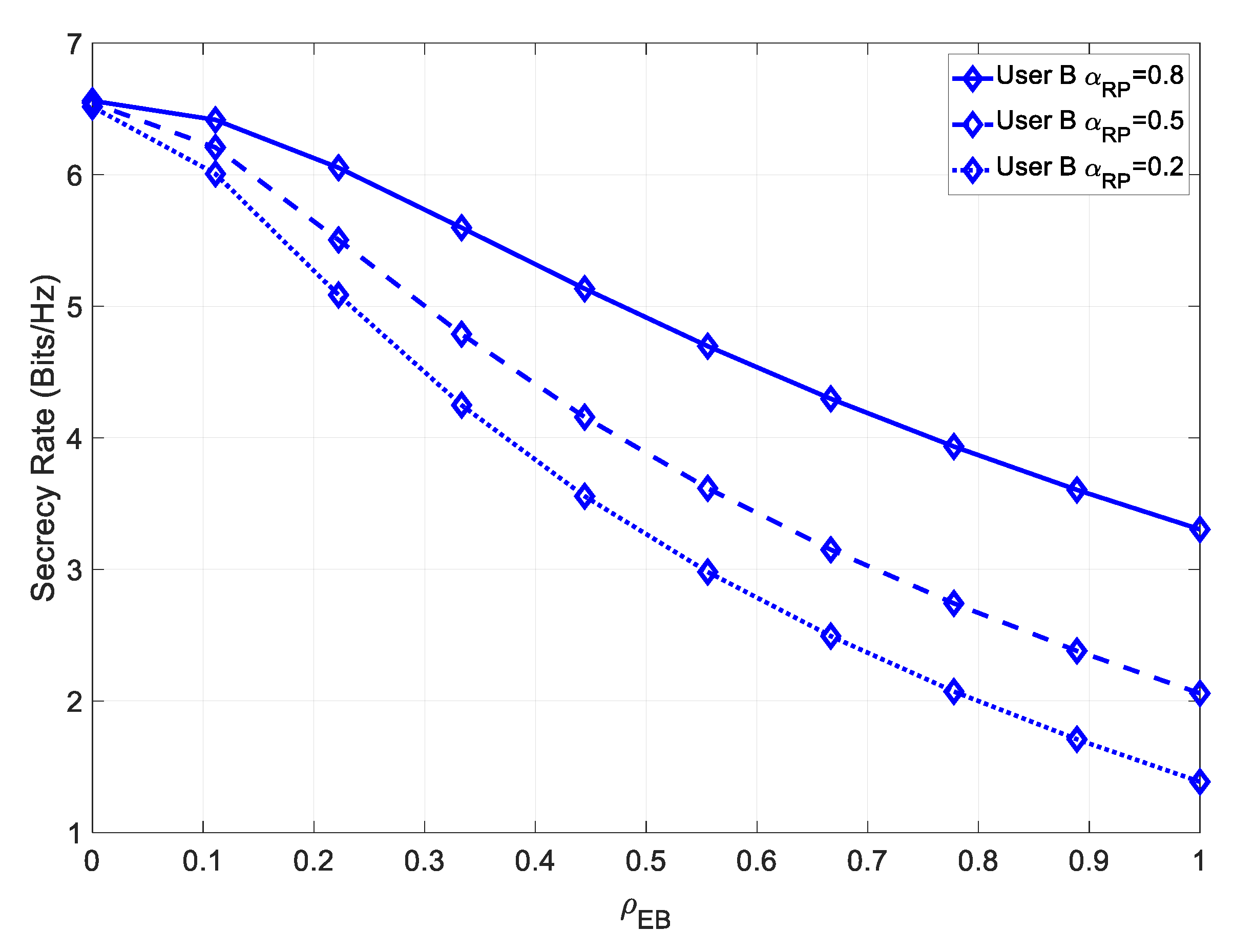
4.1.2. Line-of-Sight at User B

In this scenario, there was an LOS with all users; therefore, we analyzed the impact of the power ratio ${\alpha }_{RP}$ on the attainable secrecy rate. In Figure 8, the secrecy rate for various values of ${\alpha }_{RP}$ is shown for User B.

As expected, since the eavesdropper could not estimate the multipath component, the greater the value of ${\alpha }_{RP}$, the more secure the system could be. Figure 9 shows the secrecy rate in a scenario where there was imperfect channel estimation.

It could be observed that the channel estimation severely degraded our secrecy rate; however, even for high values of ${\rho }_{EB}$ and ${\rho }_{EC}$, the secrecy rate remained high, when compared with the non-LOS scenario, due to the multipath component. Figure 10 shows the impact of a channel mismatch error on the secrecy rate.

It could be concluded that the permanent channel mismatch error increased the secrecy rate for high values of ${\rho }_{EB}$, albeit the increase was relatively small, when compared with the non-LOS scenario. Since the lack of a multipath estimation produced a much more significant effect on the secrecy rate, then a further channel mismatch error had a smaller impact on the secrecy rate.

4.1.3. User C Results

Let us analyze the secrecy rate at the farthest user. In Figure 11, we compare the secrecy rate of User C under different levels of channel estimation error.

In this case, the maximum achievable secrecy rate was higher than the one of User B, due to the increased capacity of the channel with a higher transmit power. The effect of minimizing the channel estimation error of the receiver was significantly more noticeable in this scenario, at low values of ${\rho }_{EC}$. In Figure 12, the secrecy rate of User C is simulated under imperfect channel estimation, as well as a channel mismatch error at the eavesdropper.

It could be seen that, similarly to User B, this system achieved a higher maximum secrecy rate, at low values of ${\rho }_{EC}$, and a higher secrecy rate, even for high values ${\rho }_{EC}$.

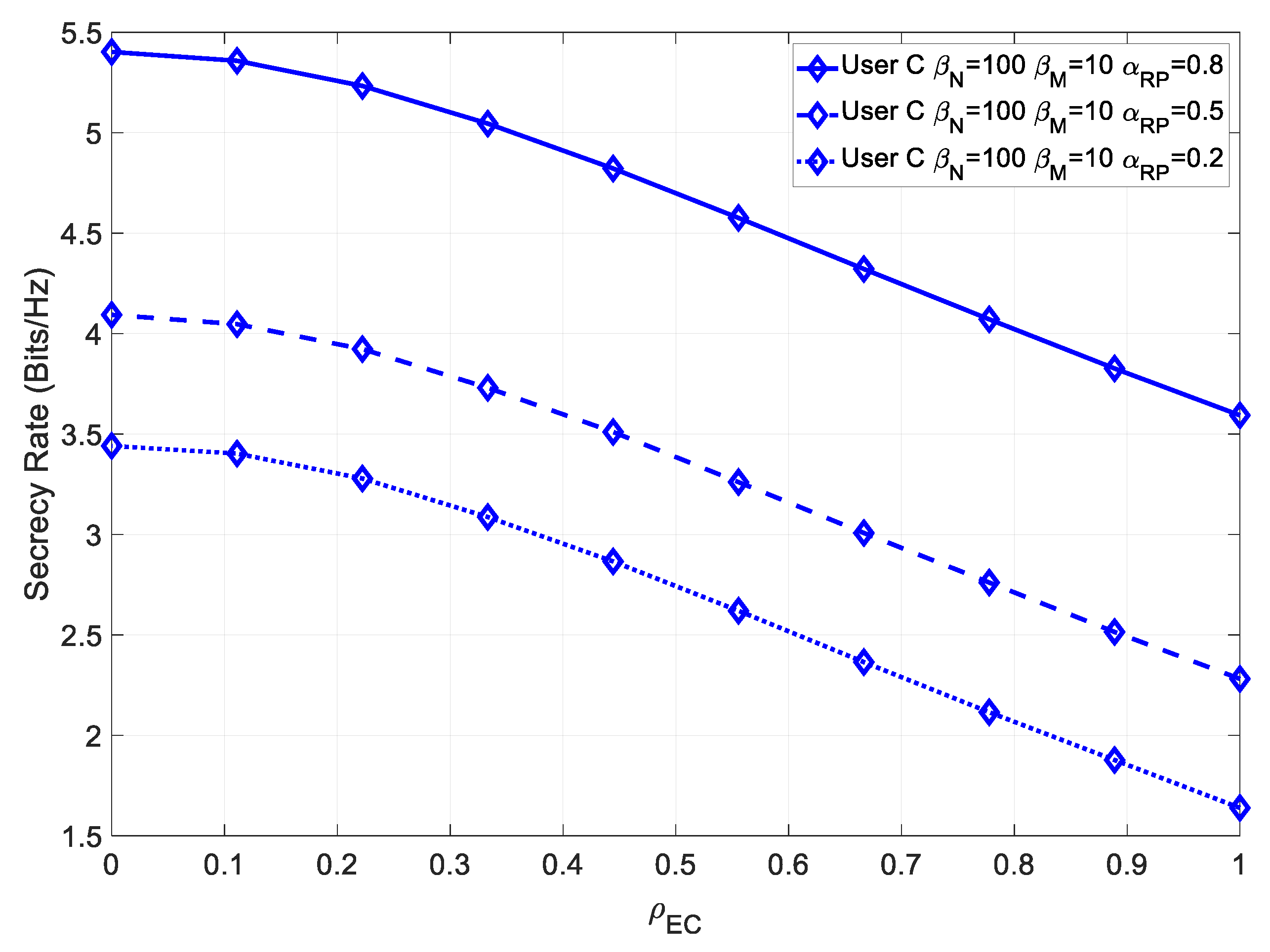
4.1.4. Line-of-Sight at User C

In the LOS scenario, we analyzed the impact of the power ratio ${\alpha }_{RP}$ on the attainable secrecy rate for user C. In Figure 13, the secrecy rate for various values of ${\alpha }_{RP}$ is shown.

Similarly, for a higher contribution of the multipath component, the achievable secrecy increased. Since in this case, there was perfect channel estimation, then User C achieved a much higher maximum secrecy rate than User B, due to its higher channel capacity. Figure 14 shows the secrecy rate for various values of ${\alpha }_{RP}$, in the presence of channel estimation errors.

In this case, the channel estimation error lowered the overall secrecy rate; however, the degradation was less severe for higher power multipath components. Moreover, it should be noted that User C’s secrecy rate was degraded much more than User B’s, as User C required very precise channel estimation. Figure 15 shows the secrecy rate for various values of ${\alpha }_{RP}$ and various sources of channel estimation errors.

As is the case for User B, the increase in the secrecy rate at high ${\rho }_{EC}$ was relatively small, compared to the NLOS scenario, as the LOS component contributed less in this scenario.

5. Conclusions

In this paper, we proposed a physical layer security level against eavesdroppers for a three user power domain MIMO-NOMA scheme based on SVD. The security potential of this scheme was studied, and it was shown that minimizing channel estimation errors and maximizing channel estimate correlations could lead to very high secrecy rates. Even in LOS scenarios, it was shown that the secrecy rate could be kept high if the multipath component’s power was relatively high. Therefore, power domain MIMO-NOMA schemes based on SVD are an attractive option for highly secure NOMA communications.