Stochastic Optimization Methods for Parametric Level Set Reconstructions in 2D through-the-Wall Radar Imaging

Abstract

In this paper, a comparison of stochastic optimization algorithms is presented for the reconstruction of electromagnetic profiles in through-the-wall radar imaging. We combine those stochastic optimization approaches with a shape-based representation of unknown targets which is based on a parametrized level set formulation. This way, we obtain a stochastic version of shape evolution with the goal of minimizing a given cost functional. As basis functions, we consider in particular Gaussian and Wendland radial basis functions. For the optimization task, we consider three variants of stochastic approaches, namely stochastic gradient descent, the Adam method as well as a more involved stochastic quasi-Newton scheme. A specific backtracking line search method is also introduced for this specific application of stochastic shape evolution. The physical scenery considered here is set in 2D assuming TM waves for simplicity. The goal is to localize and characterize (and eventually track) targets of interest hidden behind walls by solving the corresponding electromagnetic inverse problem. The results provide a good indication on the expected performance of similar schemes in a more realistic 3D setup.

1. Introduction

Through-the-wall radar imaging is a scientifically challenging imaging methodology with a large number of important applications. See for example [1] for a recent overview of this technology and some applications. The interplay between rapidly developing sensor technology and novel mathematical optimization strategies for efficient data processing makes this technology a very promising field for scientific research. A variety of practical challenges persist, though, which need to be addressed in order to extract useful information from the physically obtained data. Ideally, real-time data processing would be desired from 3D data with very limited view on the scenery hidden behind walls that significantly weaken the signal obtainable for data processing. Realistically, a trade-off might be sought between the limited view and the availability of broad-band antennas, which might provide information at various frequencies. Moreover, very often not a detailed tomographic image of the space behind the shielding walls is needed, but the goal might just be to identify and track moving objects in almost real time. This locating and tracking part appears much more feasible from limited data than a full tomographic time-resolved reconstruction.

The inverse scattering problem considered in through-the-wall radar imaging mathematically corresponds to a highly ill-posed non-linear inverse problem which is difficult to solve. Usually, iterative gradient-based pixel-by-pixel (or voxel-by-voxel in 3D) reconstruction techniques are employed which are time-consuming, slow to converge and usually suffer from local minima. One possibility to reduce complexity and reconstruction time is to employ linear approximations such as the Born or Rytov approximation instead of the full non-linear model. However, by construction those techniques cannot take into account most of the multiple-scattering effects.

Another possible way to address the complexity of the inverse scattering problem is to represent the imaging domain by a smaller set of expansion parameters using a specific model. This is the approach taken in this paper. In order to correctly represent situations of moving objects in a room, we have chosen a shape-based model represented by a small set of basis functions. The shape-based approach makes sure that the objects to be imaged can have a reasonably high contrast to the background, even though they are represented by only few expansion coefficients. The modelling of wave propagation in the same domain can still be done by any convenient wave propagation simulator, in our case a pixel-based wave simulator explained further in [2,3].

The final goal of our investigation will be the tracking of moving objects inside a given domain. This application suggests to split the reconstruction task into two subtasks, distinguishing between stationary objects which do not change from one imaging frame to the next, and the embedded moving objects which might change from one frame to the next. Therefore, in our approach we first reconstruct the background, which is assumed stationary over time, off-line as a preprocessing step (possibly updated in regular time steps) and reduce the identification and tracking part to a real-time shape reconstruction and tracking task based on a level set representation of shapes.

The splitting approach of dynamic and static objects has been presented in more details in a previous publication [4], such that we will here simply assume that the stationary background reconstruction has been completed from data obtained in previous time steps of the tracking task, and that we aim at quickly reconstructing the shape and location of a moving object from newly incoming scattering data. Both, the stationary background as well as the moving object are represented in our approach by (different) level set functions. This model can be extended if needed by also allowing for smoothly varying parameters in some background regions.

Therefore, in the present paper, our numerical setup simply consists of two empty rooms where an extended object is embedded at a given moment which needs to be characterized and located from given data. As already mentioned, since the details of the shapes represented by the level set functions are usually not of much importance in a tracking task, and due to the need of reducing dimensionality for the purpose of numerical efficiency, we adopt a particular parametric level set approach where the level set function itself is represented as a linear combination of few suitably chosen radial basis functions (RBFs). This simplification in the model enables us to adopt some specialized stochastic optimization schemes developed recently for a variety of applications. In particular, higher-order optimization approaches such as specific tailor-made versions of quasi-Newton methods for solving the numerical optimization tasks become feasible when using only few optimization parameters.

In this paper, we will present a comparison of several stochastic optimization schemes from the particular viewpoint of stochastic data selection in inverse scattering. In particular, the element of stochastic gradient selection is essential for our demonstration provided here. This is due to the following reason. Recent developments in machine learning and large-scale data analysis are indicating that also imaging, identification and tracking applications such as the one considered here might benefit from employing related stochastic approaches. This is, in particular, true since in 3D applications the amount of available data is significantly large, such that standard deterministic data processing approaches are heavily limited by computational costs of currently available numerical forward modelling tools for solving Maxwell’s equations. In the proof-of-concept study presented here, we will not directly focus on a 3D situation due to computational limitations. Instead, we consider a representative 2D setup which will allow us to get an idea about how similar methods might perform in a more realistic 3D situation. We plan to address such a more realistic 3D situation in our future research.

In this work, we compare the convergence performance of different stochastic optimization methods aimed at localizing and tracking targets of interest hidden behind walls. As mentioned, by adopting a level set description of the objects, we reduce the dimensionality of the problem by considering a parametrization scheme. This allows for the implementation of a variety of optimization algorithms. Many of these stochastic optimization techniques have been investigated recently in the framework of machine learning applications. In fact, training a neural network leads to a minimization task which benefits from fast and reliable algorithms especially in large scale problems. In addition to first order optimization schemes, in recent years there has been a significant interest in evaluating higher order techniques [5,6], which will be considered here as well. In our particular application of shape identification and tracking, we will in addition incorporate a specific line search procedure which provides smooth reconstructions without introducing high computational requirements.

The remaining parts of the paper are structured as follows. In the following Section 2, we first briefly describe the general setup of shape representation by parametrized level set functions. Then, we discuss the underlying inverse problem in mathematical terms and derive expressions for (stochastic) descent directions. Finally, we describe in this section the different stochastic optimization schemes investigated here. Section 3 is dedicated to the presentation of our numerical experiments which have been performed. We also discuss the various results and provide a comparison of our observations in that section. In Section 4, a summary and some conclusions are provided.

2. Materials and Methods

2.1. The Shape-Based Inverse Problem

2.1.1. The Forward Problem

The example setup considered here is illustrated in the left image of Figure 1. We model a 2D domain of $8\mathrm{m}\times 4\mathrm{m}$ discretized by a pixel grid of $400\times 200$ pixels each having a physical size of $2\mathrm{cm}\times 2\mathrm{cm}$. A small building is composed by two distinct rooms separated by the presence of outside and one interior walls. Each wall has a width of $10\mathrm{cm}$ and a relative permittivity of ${ϵ}_{wall}=2.0$. As already mentioned, in our study the building is considered empty for simplicity except of the targets which are assumed here to have a permittivity value ${ϵ}_{obj}=7.0$. The background space is filled with air having value ${ϵ}_0=1.0$. The conductivity is assumed constant and equal to $\sigma =0.01\mathrm{S}/\mathrm{m}$ everywhere. The conductivity and free space permittivity will not be part of the inverse problem. We mention that a more complex static background, possibly also incorporating more than one physical parameter, can be estimated in an off-line procedure by a similar process as applied here for the targets. In principle, also static and dynamic content could be reconstructed simultaneously using the same parametrised setup. However, in our opinion, it does make sense to separate those different content types and use different level set representations for the background and for the targets. Therefore, in this paper, we will only consider the dynamic tracking part. Actually, we only consider one given time step of this dynamic estimation, where the dynamic aspect is only considered as a constraint in available processing time for obtaining a fast approximate estimation of the location of a target. We will not explicitly incorporate correlations over time between different frames, as it can be done by making use of Kalman Filter techniques for example. Those have been addressed in different publications, see for example [2,4]. We plan to combine those different aspects of a time-dependent inverse problem in our future research. Moreover, we refer the reader for more details on how to estimate the static background distribution to our earlier publications, in particular [3,7,8,9].

In our computational setup for evaluating and comparing the different schemes, the building is surrounded by a set of antennas which act as sources and receivers of electromagnetic radiation. Each antenna operates at a given selection of frequency values, which in our numerical experients will be $f=\{100,150,200,250,300\}\mathrm{MHz}$. For the mathematical model used to describe the propagation of the fields within the domain, we consider Transverse Magnetic (TM) waves which propagate according to the Helmholtz equation

$$\Delta u+\kappa u=q$$

(1)

equipped with a Sommerfeld radiation condition [2,3,8]. Here, u describes one component of the electric field, q represents the external sources (i.e., the antennas) and the complex parameter $\kappa$ is connected to the wavenumber k as

$$\kappa =k^2={\omega }^2{\mu }_0{ϵ}_0ϵ+i\omega {\mu }_0\sigma ,$$

(2)

where ${ϵ}_0$ is the dielectric permittivity in free space, ${\mu }_0$ is the magnetic permeability in free space and $\omega =2\pi f$ is the angular frequency.

A 2D Finite Differences Frequency Domain (FDFD) discretization of this Helmholtz model equipped with Perfectly Matched Layers (PMLs) [10] is used in our numerical experiments. This code is similar to the one described in [2] and runs on a standard workstation in our simulations.

We consider the presence of p sources $q_j,j=1,\dots ,p$ and D receivers located at ${\mathbf{x}}_d,d=1,\dots ,D$. Let ${\tilde{G}}_{jk}\in {\mathbb{C}}^D$ be the measurement data collected for a source $q_j,j=1,\dots ,p$ and a frequency $f_k,k=1,\dots ,K$. For a given permittivity profile $ϵ$, we can use the Helmholtz model to approximate the corresponding fields. These fields can be evaluated at the receiver locations by introducing a measurement operator as follows:

$$M{u}_{jk}={(u_{jk}({\mathbf{x}}_1),\dots ,u_{jk}({\mathbf{x}}_D))}^T,$$

(3)

where we denote by $u_{jk}$ the solution of Equation (1) for a given source $q_j$ and frequency $f_k$. Therefore, we can define the residual operator

$$R_{jk}(ϵ)=M{u}_{jk}(ϵ)-{\tilde{G}}_{jk},$$

(4)

for a given source and frequency. In the derivation provided in following sections, we will also often combine all residual functions $R_{jk}(ϵ)$ in a vector quantity $R(ϵ)$. Standard techniques for addressing the underlying inverse problem are based on determining descent directions of a well-designed cost functional based on those quantities $R_{jk}$.

2.1.2. Level Set Representation of Shapes

The level set method [11,12,13] for shape representation and reconstruction has been introduced in the inverse problems community by [14] and has been further developed since then for a variety of electromagnetic inverse problems. A recent overview can be found in [7,9]. As part of this development, the specific use of parametric level sets has been proposed at an early stage in the electromagnetic imaging community, see for example [15]. The parametric approach helps to reduce the dimensionality of the underlying optimization problem and is useful for applying further regularization for the imaging task. This approach has also found applications beyond electromagnetic inversion, for example in seismic imaging [16].

Whereas more traditional pixel-based level set methods have the potential to yield high accuracy and flexibility for shape representations [3,7], they also suffer from some drawbacks. For example, due to computational constraints, usually only first order methods are applied in the underlying optimization task which might yield long evolution processes. Moreover, a fine grid (i.e., a large number of pixels) is generally required to achieve an accurate representation, which might imply high memory requirements and computational efforts [17]. The parametric level set approach attempts to mitigate some of those difficulties, for the price of a potentially less detailed shape representation. In the following, we provide a very brief overview of the parametric level set method and its use for describing objects embedded within a domain for electromagnetic imaging.

In the parametric level set method, each object is represented by a smooth level set function $\varphi$ which, instead of being defined directly on a pixel grid, is conveniently expressed in terms of a smaller set of suitably chosen basis functions (the latter ones being defined on the pixel grid). This generally reduces the number of unknowns involved, which also comes with an implicit regularization effect [15]. Since the properties of the basis functions used can be chosen to guarantee the stability and the smoothness of the solution, the addition of further regularization terms in the cost functional often can be avoided.

Following [15], let us consider a closed domain $D\subseteq {\mathbb{R}}^2$ with corresponding boundary $\partial D$ and a coefficient vector $\mathit{\mu }=({\mathit{\mu }}_1,\dots ,{\mathit{\mu }}_m)\in {\mathbb{R}}^m$. A level set representation of D can be obtained by considering a smooth level set function $\varphi (\mathbf{x},\mathit{\mu }):{\mathbb{R}}^2\times {\mathbb{R}}^m\to \mathbb{R}$ such as

$$\left\{\begin{array}{c}\varphi (\mathbf{x};\mathit{\mu })>c,\forall \mathbf{x}\in D,\hfill \\ \varphi (\mathbf{x};\mathit{\mu })=c,\forall \mathbf{x}\in \partial D,\hfill \\ \varphi (\mathbf{x};\mathit{\mu })<c,\forall \mathbf{x}\in {\mathbb{R}}^2\backslash D,\hfill \end{array}\right.$$

(5)

where $c\in \mathbb{R}$ is chosen conveniently (a typical choice is $c=0$). The coefficient vector $\mathit{\mu }$ refers to expansion coefficients with respect to the chosen set of basis functions, which in our case will be RBFs (radial basis functions). Therefore, in the parametric approach each permissible shape D has to be represented by a specific choice of expansion vector $\mathit{\mu }$. A shape evolution reduces to the evolution of this expansion vector $\mathit{\mu }$ over artificial evolution time. When using a discretized evolution time, this resembles a discrete optimization approach for $\mathit{\mu }$ [7].

2.1.3. Calculation of Descent Directions

Let us assume that we are interested in recovering an unknown (physical) parameter function $p(\mathbf{x})\in {\mathbb{S}}_p$ (in our case representing the real-valued electric permittivity), where

$${\mathbb{S}}_p:=\left\{p:{\mathbb{R}}^2\to \mathbb{R},{\int }_{{\mathbb{R}}^2}{\left|p\right|}^{2}d\mathbf{x}<\infty \right\}$$

(6)

is a space equipped with inner product

$${\langle p_1,p_2\rangle }_{{\mathbb{S}}_p}={\int }_{{\mathbb{R}}^2}{p}_1(\mathbf{x})p_2(\mathbf{x})d\mathbf{x}.$$

(7)

In the parametric level set formulation, furthermore, the problem can be written as follows

$$p(\mathbf{x};\mathit{\mu })=p_i(\mathbf{x})H(\varphi (\mathbf{x};\mathit{\mu })-c)+p_o(\mathbf{x})(1-H(\varphi (\mathbf{x};\mathit{\mu })-c)),$$

(8)

where $\mathit{\mu }$ is a vector containing expansion coefficients with respect to a given set of basis functions. Specific choices will be specified further below. Here, $H(·)$ denotes the Heaviside function, $\varphi$ denotes the level set function representing the shape D of interest, and $p_i(\mathbf{x})$, $p_o(\mathbf{x})$ are the a-priori known profiles of the sought property inside and outside D, respectively. Note that Equation (8) implies that $p(\mathbf{x};\mathit{\mu })$ is not differentiable in the classical sense along $\partial D$, since the Heaviside function is not differentiable in standard function spaces. This reflects the discontinuity of the parameter function p across $\partial D$. However, if interpreting the Heaviside function in the framework of mathematical distribution theory, we formally can still differentiate $p(\mathbf{x};\mathit{\mu })$. See for more details again [7]. On the other hand, the two functions $p_o(\mathbf{x})$ and $p_i(\mathbf{x})$ can follow quite a complex pattern even though in our numerical experiments both are specified by simple prior distributions representing a constant inside the target and a building filled with air outside of it.

Considering the expansion coefficients $\mathit{\mu }$ as the fundamental unknown of the underlying inverse problem, we define now the cost functional as

$$J(\mathit{\mu }):{\mathbb{R}}^m\to \mathbb{R},J(\mathit{\mu })=\frac{1}{2}{\left|\right|R(\mathit{\mu })\left|\right|}_2^2$$

(9)

which needs to be minimized with respect to $\mathit{\mu }$. Following classical optimization theory, and abusing slightly notation by using the same symbol R in two different function spaces, this cost functional is suitably defined in terms of a residual operator $R(\mathit{\mu })=R(p(\mathbf{x};\mathit{\mu }))$, which provides the discrepancy between our current estimation and the true profile of p. The variation of the cost with respect to the parameter $\mathit{\mu }$ (or its components ${\mathit{\mu }}_j$) is formally obtained by the chain rule

$$\frac{\partial J}{\partial {\mathit{\mu }}_j}=\frac{\partial J}{\partial p}\left[\frac{\partial p}{\partial {\mathit{\mu }}_j}\right].$$

(10)

Each factor appearing on the right of Equation (10) is investigated separately hereafter.

Expressing the residual operator $R(p)$ in terms of the unknown property $p(\mathbf{x})$ (dropping its dependence of $\mathit{\mu }$ in this part for simplicity of notation), we start by computing $R(p+ϵ\delta p)$, where $ϵ\in \mathbb{R}$ is a small parameter and $\delta p\in {\mathbb{S}}_p$ is an arbitrary variation. We denote by $R^{\prime }(p)$ the linearized residual operator of $R(p)$, assuming that it exists and is well defined. This operator is expected to satisfy the generalized Taylor expansion

$$R(p+ϵ\delta p)=R(p)+ϵR^{\prime }(p)\left[\delta p\right]+O({ϵ}^2)$$

(11)

in an appropriate sense and with suitably chosen function spaces. We refer for more details to [3,18,19]. Following the derivations in [3,18,19], we can conclude that

$$\frac{\partial J}{\partial p}\delta p=J^{\prime }(p)\left[\delta p\right]=\mathrm{Re}{\langle R^{\prime }{(p)}^{\ast }\left[R(p)\right],\delta p\rangle }_{{\mathbb{S}}_p},$$

(12)

where the symbol Re indicates to take the real part of the following quantity and $R^{\prime }{(p)}^{*}$ denotes the adjoint of the linearized operator $R^{\prime }(p)$ (with respect to the given function spaces which are not specified here further).

Let us move our attention now towards the second factor in Equation (10). Since $\frac{\partial p}{\partial {\mathit{\mu }}_j}=\frac{\partial p}{\partial \varphi }\frac{\partial \varphi }{\partial {\mathit{\mu }}_j}$ where $\frac{\partial p}{\partial \varphi }=(p_i-p_o)\delta (\varphi -c)$ from Equation (8), and recalling Equation (12), we can express Equation (10) as

$$\frac{\partial J}{\partial {\mathit{\mu }}_j}=\mathrm{Re}{\langle R^{\prime }{(p)}^{*}\left[R(p)\right],(p_i-p_o)\delta (\varphi -c)\frac{\partial \varphi }{\partial {\mathit{\mu }}_j}\rangle }_{{\mathbb{S}}_p}$$

(13)

where $\delta (·)$ denotes the Dirac delta function (or ‘delta distribution’ to be more precise). The factor $\frac{\partial \varphi }{\partial {\mathit{\mu }}_j}$ depends on the specific choice of radial basis function and is calculated once this choice has been made. This will be done in the following section.

2.1.4. Specific Choice of Basis Functions

So far, we have not yet specified which basis functions we will choose in our schemes. Standard choices are RBFs due to many convenient properties. Some details about those basis functions used to parametrize the level set function $\varphi$ are provided next. The selection of a suitable class of basis functions should take into account the features of the objects to be represented. For example, this class should be able to describe boundaries with different typical curvatures. Therefore, the choice of RBFs may affect the capability of the technique to retrieve details with a specific geometry [15,16].

We will focus our attention on the following two classes of RBFs [20]:

$$\begin{array}{cc}\hfill (i)& \mathrm{Gaussian} \mathrm{functions} (\mathrm{GA}):\psi (r)={\mathrm{e}}^{-{(\theta r)}^2};\\ \hfill (ii)& {\mathrm{Wendland}}^{’}\mathsf{s} \mathrm{functions} (\mathrm{WL}):\psi (r)={(1-\frac{r}{\delta })}_{+}^4(4\frac{r}{\delta }+1).\end{array}$$

Here, $r=\left|\right|\mathbf{x}-{\mathit{\chi }}_0{\left|\right|}_2$ is the Euclidean distance between a generic point $\mathbf{x}$ of the domain and the centre ${\mathit{\chi }}_0$ of the considered RBF. Moreover, $\theta ,\delta \in {\mathbb{R}}^{+}$ are free parameters that control the shape of $\psi (r)$. For brevity, we have introduced the notation

$${\left(1-\frac{r}{\delta }\right)}_{+}^4=\left\{\begin{array}{c}{(1-\frac{r}{\delta })}^4,\mathrm{if}0\le \frac{r}{\delta }<1,\hfill \\ 0,\mathrm{otherwise}.\hfill \end{array}\right.$$

(14)

The Wendland’s functions are a common example of Compactly Supported Radial Basis Functions (CSRBFs), since they only have nonzero contributions inside a disc of radius $\delta$ around their centres [15]. Gaussian RBFs, on the other hand, have nonzero contributions at each location of the considered domain. This is the main distinguishing feature between the above two classes considered here.

According to [15], a common strategy to achieve high flexibility is to express $\varphi$ as a linear combination of RBFs of the type:

$$\varphi (\mathbf{x};\mathit{\mu },\mathit{\chi })=\sum _{j=1}^m{\mathit{\mu }}_j\psi (||(\mathbf{x}-{\mathit{\chi }}_j){\left|\right|}_2),$$

(15)

where $\mathit{\mu }\in {\mathbb{R}}^m$ is a coefficient vector and ${\mathit{\chi }}_j\in {\mathbb{R}}^2$ denotes the centre of the j-th RBF. Throughout the numerical part of this work, these centres are fixed and uniformly distributed in the domain. Those assumptions can be relaxed in future work. Obviously, from the above expression Equation (15), we see immediately that

$$\frac{\partial \varphi }{\partial {\mu }_j}=\psi (||(\mathbf{x}-{\mathit{\chi }}_j){\left|\right|}_2)$$

(16)

which is the final building block needed for calculating the right hand side of Equation (13).

2.1.5. Shape Evolution Schemes

We are now able to express the evolution of a standard (deterministic) gradient based shape reconstruction algorithm in terms of an iterative update of the coefficient vector $\mathit{\mu }$ as follows:

$$\left\{\begin{array}{c}{\mathit{\mu }}_t={\mathit{\mu }}_{t-1}-{\eta }_t{\nabla }_{\mathit{\mu }}{J(\mathit{\mu })|}_{\mathit{\mu }={\mathit{\mu }}_{t-1}},\hfill \\ {\mathit{\mu }}_0={\mathit{\mu }}^{(0)},\hfill \end{array}\right.$$

(17)

for $t=1,2,\dots$, where ${\eta }_t$ is the step size amplitude at iteration t and starting point ${\mathit{\mu }}^{(0)}$. Notice that the calculation of the update Equation (17) requires us to take into account the gradient ${\nabla }_{\mathit{\mu }}J(\mathit{\mu })$ with respect to the entire data set, which can be computationally demanding in many practical situations. Further below, we will describe the stochastic approach, which divides this task into small subtasks in a stochastic fashion.

One of the main advantages introduced by the parametric representation is that, due to the reduction of the dimensionality of the problem, faster (than linear) converging schemes can be explored on standard computing architecture to minimize the cost function. The application of so-called quasi-Newton or Newton methods can increase the converge rate and, therefore, speed up the reconstruction of the unknown property $p(\mathbf{x})$. However, at the same time, they generally imply an increase in the computational complexity and therefore a trade-off may be necessary.

Further below, we will also introduce a stochastic quasi-Newton method to approximate the true Hessian $\mathit{H}(\mathit{\mu })$ of the cost function by using information given by zero- and first-order derivatives. This is in contrast with the procedure followed in [15], where an analytical approximation of the Hessian is derived. Our approach provides a matrix $\tilde{\mathit{H}}(\mathit{\mu })$ which can be used to compute an update direction $\Delta {\mathit{\mu }}_t={\mathit{\mu }}_t-{\mathit{\mu }}_{t-1}$ for the coefficient vector ${\mathit{\mu }}_{t-1}$ by solving the following Levenberg–Marquardt system:

$${\left[\tilde{\mathit{H}}(\mathit{\mu })\right|}_{\mathit{\mu }={\mathit{\mu }}_{t-1}}+\lambda \mathit{I}{]\Delta {\mathit{\mu }}_t=-{\nabla }_{\mathit{\mu }}J(\mathit{\mu })|}_{\mathit{\mu }={\mathit{\mu }}_{t-1}},$$

(18)

with $\lambda \ge 0$. More details are given in the next section.

2.2. Stochastic Optimization Algorithms

In this section, we introduce the optimization algorithms analysed in this study. As already mentioned, calculating the full Jacobian or Hessian is considered too expensive in our application. However, we want to take advantage of a specific structure of our data set. In our particular numerical setup in 2D, we face the situation that it is straightforward to calculate all gradient information for a fixed frequency, but that this computational effort needs to be done as many times as there are different frequencies used in a multi-frequency setup. Therefore, we would like to design an iterative optimization scheme which provides us with an update for the parameters after having processed all information related to one single frequency, before moving on to processing the next available frequency information. This will be done in a stochastic fashion. For more general 3D situations (considered in our ongoing work), we might prefer to choose different subsets of data instead. For example, the use of a typical Maxwell simulator in 3D might suggest to combine all data related to a fixed emitting sensor location. This indicates that the decision on how to divide the data set into smaller parts is partially linked to the choice of the available numerical simulators.

As already mentioned, the goal is to localize targets of interest by recovering the permittivity profile $ϵ$ within the domain starting from measurements collected by antennas operating at different frequencies $f_k,k=1,\dots ,K$. This is done by minimizing a cost function defined as the sum of contributions corresponding to different data subsets (here different frequencies). Standard optimization techniques require to compute the gradient of this cost which, due to its structure, might result in an expensive procedure especially for large scale problems.

An alternative way to proceed consists in successively approximating the full gradient by considering only a subset of data at a time. By selecting this subset randomly and by updating the unknown parameter $ϵ$ along the direction given by this gradient approximation, it is possible to efficiently reduce and ideally minimize the cost functional keeping the computational requirements limited. This approach leads to the development of first-order stochastic optimization schemes which have been proved to perform well in many contexts, including machine learning applications [21,22].

The introduction of stochastic approaches increases the efficiency but, on the other hand, produces some complications. For example, monitoring the full cost trend provides a viable modality to assess the evolution of an algorithm. In stochastic contexts, however, this strategy cannot be directly applied simply because the full gradient is not available. Therefore, even though our implemented stochastic approaches consider only a single frequency per iteration, we decide to periodically evaluate the full cost by considering the contributions of all frequencies for monitoring purposes. In order not to overly reduce the efficiency of our schemes, we perform this control calculation only every $N_{cost}$ iterations. Similarly, the definition of a robust stopping criterion in a stochastic framework is a problem that is difficult to address. In this study, we simply monitor the trend of the global cost (as evaluated in these additional control steps) and stop the simulation after a fixed number of iterations. The development of more sophisticated stopping criteria will be addressed in our future research.

Besides the specific line search scheme described further below, we will be able to apply stochastic optimization schemes very similar to their standard form as described extensively in the available literature. The main difference of our application to the available standard literature is the fact that we recover a level set function represented by radial basis functions, which however, is not the actual target of the optimization task itself. Instead we are interested in the shapes represented by that level set function, which is a new interpretation of the results of such stochastic schemes. In a certain sense, we are designing a stochastic shape evolution scheme based on available stochastic optimization approaches. The use of stochastic shape evolution by a level set representation of shapes has been applied previously to optimal engineering design problems, see for example [23] and references provided there. One advantage mentioned in those applications is that stochastic approaches might help circumvent certain local minima which might occur in deterministic shape optimization approaches. This advantage might also be expected in our novel application presented here when solving electromagnetic inverse problems in the application of through-the-wall radar imaging. However, this is not the focus of this paper and we will not investigate this property in more details here.

2.2.1. A Line Search Scheme for Stochastic Shape Optimization

Most optimization approaches require some thoughts regarding efficient line search criteria. For our particular schemes considered here, we consider a line search strategy which is tailor-made for shape evolution problems, in particular in conjunction with level set representations of shapes. In stochastic frameworks, standard gradient-based line search criteria such as the Wolfe or Armijo condition are not possible to use since the full gradient of the cost is not easily available [24]. Therefore, we adopt a specific backtracking procedure where no additional run of our forward simulator is required [25,26,27]. Instead, it focuses on obtaining a controlled speed of the underlying shape evolution, measured by the number of pixels that change value in one given time step. Despite its computational efficiency, this line search (as many others derived for stochastic approaches) does not enforce explicitly the reduction of the cost in each step. Therefore, temporary increases of the cost value might occur as the algorithm proceeds. On the other hand, this relaxed treatment of the actual cost might be beneficial for avoiding certain local minima, as already mentioned above.

A fairly smooth shape evolution throughout the reconstruction is ensured and its speed controlled by exploiting the pixel representation of the shapes in the domain. In fact, at each step, we require that the number of pixels (or voxels in a 3D setup) $N_{vox}$ that change the value of their permittivity due to shape updates is always included in a given interval $I_{vox}=[N_{vox}^{min},N_{vox}^{max}]$. The selection of this interval is realized such that $N_{vox}^{min}$ is large enough to guarantee that sufficient progress is made at each iteration whilst $N_{vox}^{max}$ is small enough to avoid overshooting. The line search method employed here is outlined in Algorithm 1. More details can be found in [25].

Algorithm 1: Shape-based line search scheme.

Let ${\mathit{\mu }}_t$ and $\Delta {\mathit{\mu }}_{t+1}$ be the coefficient vector at iteration t and the new update direction

Compute the level set function ${\varphi }_t$ associated with ${\mathit{\mu }}_t$    (Equation (15))

Compute the permittivity profile ${ϵ}_t$ associated with ${\mathit{\mu }}_t$    (Equation (8))

Initialize the line search parameter ${\eta }_t={\eta }_0$, where ${\eta }_0>0$

Define the parameters ${\alpha }_1,{\alpha }_2$ such that $0<{\alpha }_1<1$ and ${\alpha }_2>1$

Define the interval $I_{vox}=[N_{vox}^{min},N_{vox}^{max}]$

while ($N_{vox}\notin I_{vox}$) do

$\tilde{\mathit{\mu }}={\mathit{\mu }}_t+{\eta }_t\Delta {\mathit{\mu }}_{t+1}$    % trial coefficient vector

Compute the corresponding level set function $\tilde{\varphi }$    (Equation (15))

Compute the corresponding permittivity profile $\widetilde{ϵ}$    (Equation (8))

Count the number $N_{vox}$ of pixels where $(\widetilde{ϵ}-{ϵ}_t)\ne 0$

if ($N_{vox}<N_{vox}^{min}$) then

${\eta }_t={\alpha }_2{\eta }_t$

end if

if ($N_{vox}>N_{vox}^{max}$) then

${\eta }_t={\alpha }_1{\eta }_t$

end if

end while

return${\eta }_t$

2.2.2. A Stochastic Gradient Descent Algorithm

In this section, we briefly describe the popular Stochastic Gradient Descent (SGD) method for optimization. We will mainly follow the exposition provided in [28,29] and refer for more details to those publications.

Due to the structure of the cost function $J(\mathit{\mu })$, the computation of its gradient requires a loop over all (frequency) data. This is generally an expensive procedure, especially for large scale problems. Therefore, with the aim of increasing efficiency, SGD randomly selects a subset of data and approximates the computation of the gradient by a version which only takes into account this particular subset of data. According to [28,29], the main idea is that the iterative updates along the directions defined by the successive approximations to the gradient yield an average behaviour that replicates the application of standard (batch) gradient descent methods when the number of sweeps considered is sufficiently high.

The structure of the algorithm as implemented here is illustrated in Algorithm 2.

2.2.3. The Adam Algorithm

The Adam algorithm [30] is a generalization of the SGD method which takes into account low-order moments of the gradients. It has become a popular optimization algorithm commonly used nowadays to train neural networks in machine learning applications. We follow here the paper [30] and refer for more details to that publication. The popularity of the method is mainly due to its memory and computational efficiency, to its fast convergence and to its applicability in high dimensional parameter problems.

Algorithm 2: SGD algorithm.

Initialize the parameter vector ${\mathit{\mu }}_0$

Initialize the level set function ${\varphi }_0$

$t=0$

while$\mathit{\mu }$ not converged do

$t=t+1$

Randomly extract a data subset ${\mathit{X}}_{t-1}$ from the dataset $\mathit{X}$

Compute the gradient of the cost wrt ${\mathit{X}}_{t-1}$: ${\nabla }_{\mathit{\mu }}J({\mathit{\mu }}_{t-1},{\mathit{X}}_{t-1})$

Update the coefficient vector: ${\mathit{\mu }}_t={\mathit{\mu }}_{t-1}-{\eta }_t{\nabla }_{\mathit{\mu }}J({\mathit{\mu }}_{t-1},{\mathit{X}}_{t-1})$

where ${\eta }_t>0$ is chosen according to the line search Algorithm 1

end while

Compute the final level set $\varphi$ and the corresponding permittivity profile $ϵ$

Recalling the cost function $J(\mathit{\mu })$ defined before, the main idea is to iteratively update the unknown parameter vector $\mathit{\mu }$ along gradient descent directions for $J(\mathit{\mu })$ computed with respect to random subsets of training data. However, compared to SGD, here the performance is further boosted by adopting adaptive learning rates starting from estimates of the first and second gradient moment. As mentioned, the structure of the algorithm implemented here follows roughly [30], where a general mathematical analysis including convergence details is provided. However, in order to adjust the algorithm to our particular application to shape optimization, we equip it with the line search scheme provided in Algorithm 1. This combination results in our version of the Adam method outlined in the pseudo-code of Algorithm 3. Notice that the parameter $\alpha$ in Algorithm 3 has been introduced to improve the stability of the method [30]. In our numerical experiments, we have empirically chosen the value $\alpha ={10}^{-8}$.

Algorithm 3: Adam algorithm.

Initialize the parameter vector ${\mathit{\mu }}_0$

Initialize the level set function ${\varphi }_0$

Define the exponential decay rates for the moment estimates: ${\beta }_1,{\beta }_2\in [0,1)$

Initialize the first moment vector ${\mathit{m}}_0=\mathbf{0}$

Initialize the second moment vector ${\mathit{v}}_0=\mathbf{0}$

$t=0$

while$\mathit{\mu }$ not converged do

$t=t+1$

Randomly extract a data subset ${\mathit{X}}_{t-1}$ from the dataset $\mathit{X}$

Compute the gradient of the cost wrt ${\mathit{X}}_{t-1}$: ${\mathit{g}}_t={\nabla }_{\mathit{\mu }}J({\mathit{\mu }}_{t-1},{\mathit{X}}_{t-1})$

Update the first moment vector ${\mathit{m}}_t={\beta }_1{\mathit{m}}_{t-1}+(1-{\beta }_1){\mathit{g}}_t$

Update the second moment vector ${\mathit{v}}_t={\beta }_2{\mathit{v}}_{t-1}+(1-{\beta }_2){\mathit{g}}_t^2$, where ${\mathit{g}}_t^2$ denotes the elementwise square of ${\mathit{g}}_t$

Rescale the first moment vector ${\widehat{\mathit{m}}}_t={(1-{\beta }_1^t)}^{-1}{\mathit{m}}_t$

Rescale the second moment vector ${\widehat{\mathit{v}}}_t={(1-{\beta }_2^t)}^{-1}{\mathit{v}}_t$

Update the coefficient vector: ${\mathit{\mu }}_t={\mathit{\mu }}_{t-1}-{\eta }_t{\widehat{\mathit{m}}}_t/(\sqrt{{\widehat{\mathit{v}}}_t}+\alpha )$, where $\alpha >0$

and ${\eta }_t>0$ is chosen according to the line search Algorithm

end while

Compute the final level set $\varphi$ and the corresponding permittivity profile $ϵ$

2.2.4. The Online BFGS Algorithm

Finally, we describe a stochastic version of a quasi-Newton method which is the third technique considered in this work. In general, classical quasi-Newton methods aim to approximate second-order derivative information by combining gradient information from sequential updates in an iterative fashion. This requires some adjustments in the stochastic setting making sure that successive gradients used for this approximation are in fact related to each other. In Algorithm 4, which is generally motivated by the approach described in [31], we present a stochastic variation of the popular BFGS method [32,33] which is implemented in our numerical experiments.

Algorithm 4: oBFGS algorithm.

Initialize the parameter vector ${\mathit{\mu }}_0$

Initialize the level set function ${\varphi }_0$

Initialize the parameters: $c\in (0,1]$, $\lambda \ge 0$, $\alpha >0$

Initialize the inverse Hessian approximation of the cost: ${\mathit{B}}_0=\alpha \mathit{I}$

$t=0$

while$\mathit{\mu }$ not converged do

Randomly extract a data subset ${\mathit{X}}_t$ from the dataset $\mathit{X}$

${\mathit{p}}_t=-{\mathit{B}}_t{\nabla }_{\mathit{\mu }}J({\mathit{\mu }}_t,{\mathit{X}}_t)$

Update the coefficient vector: ${\mathit{\mu }}_{t+1}={\mathit{\mu }}_t+{\mathit{s}}_t$, where ${\mathit{s}}_t={\eta }_t{\mathit{p}}_t$

with ${\eta }_t>0$ chosen according to the line search Algorithm

${\mathit{y}}_t={\nabla }_{\mathit{\mu }}J({\mathit{\mu }}_{t+1},{\mathit{X}}_t)-\nabla J_{\mathit{\mu }}({\mathit{\mu }}_t,{\mathit{X}}_t)+\lambda {\mathit{s}}_t$

if (t=0) then

${\mathit{B}}_t=\frac{{\mathit{s}}_t^T{\mathit{y}}_t}{{\mathit{y}}_t^T{\mathit{y}}_t}\mathit{I}$

end if

${\rho }_t={({\mathit{s}}_t^T{\mathit{y}}_t)}^{-1}$

${\mathit{B}}_{t+1}=(\mathit{I}-{\rho }_t{\mathit{s}}_t{\mathit{y}}_t^T){\mathit{B}}_t(\mathit{I}-{\rho }_t{\mathit{y}}_t{\mathit{s}}_t^T)+c{\rho }_t{\mathit{s}}_t{\mathit{s}}_t^T$

$t=t+1$

end while

Compute the final level set $\varphi$ and the corresponding permittivity profile $ϵ$

Again, Algorithm 4 differs from the one presented in [31] by the novel line search procedure adjusted to our shape optimization task. In [31], no line search is introduced since the required convexity of the object function ensures that the curvature condition ${\mathit{s}}^T\mathit{y}\ge 0$ holds. However, since in our problem, this convexity is not guaranteed a-priori, we empirically introduce the explicit line search specified by Algorithm 1.

As already mentioned, some further consideration is needed regarding the approximation of second-order derivative information. This is so since successively calculated gradient directions for stochastically selected data subsets do not necessarily provide information regarding the second-order derivatives of the entire data set, or regarding the individual data subsets. Therefore, the stochastic approach requires the calculation of two distinct gradients per iteration for a given data subset, whereas the deterministic BFGS can make use of two successively calculated gradients from different iterations instead. This shows that the direct extension of the deterministic quasi-Newton method towards a stochastic framework requires some particular adjustments [34]. In particular, due to the definition of ${\mathit{y}}_t$ in Algorithm 4, it is essential that these two gradients are calculated with respect to the same subset of data to preserve stability.

In addition it should be mentioned that the oBFGS algorithm proposed in [31] has been developed specifically for convex functions. The cost functionals considered in our applications are not expected to be convex globally. However, it might be assumed that, when starting this scheme sufficiently close to a local minimum, the local approximation can be assumed as convex. Therefore, we can try to circumvent this limitation by choosing a starting point sufficiently close to a local minimum of the cost functional. This is the reason why we usually start the reconstruction with oBFGS after having performed a fixed number of iterations with first-order methods, in particular here the Adam method, before switching to oBFGS once the cost value has been reduced sufficiently. With a sufficiently low cost value, we expect that the algorithm has reached the vicinity of a local minimum which justifies the use of oBFGS locally.

Finally, inspired by the restarting procedure developed for the conjugate gradient method [35,36], we have also taken into account a small modification of the oBFGS algorithm which reinitializes the (inverse) Hessian approximation by the identity matrix every $N_{ReIni}$ sweeps. This is a popular technique in numerical optimization to make sure that the local quadratic approximation to the cost functional is well retrieved by the individual Hessian updates [37]. A performance comparison between these two oBFGS variants is included as well in the following numerical section.

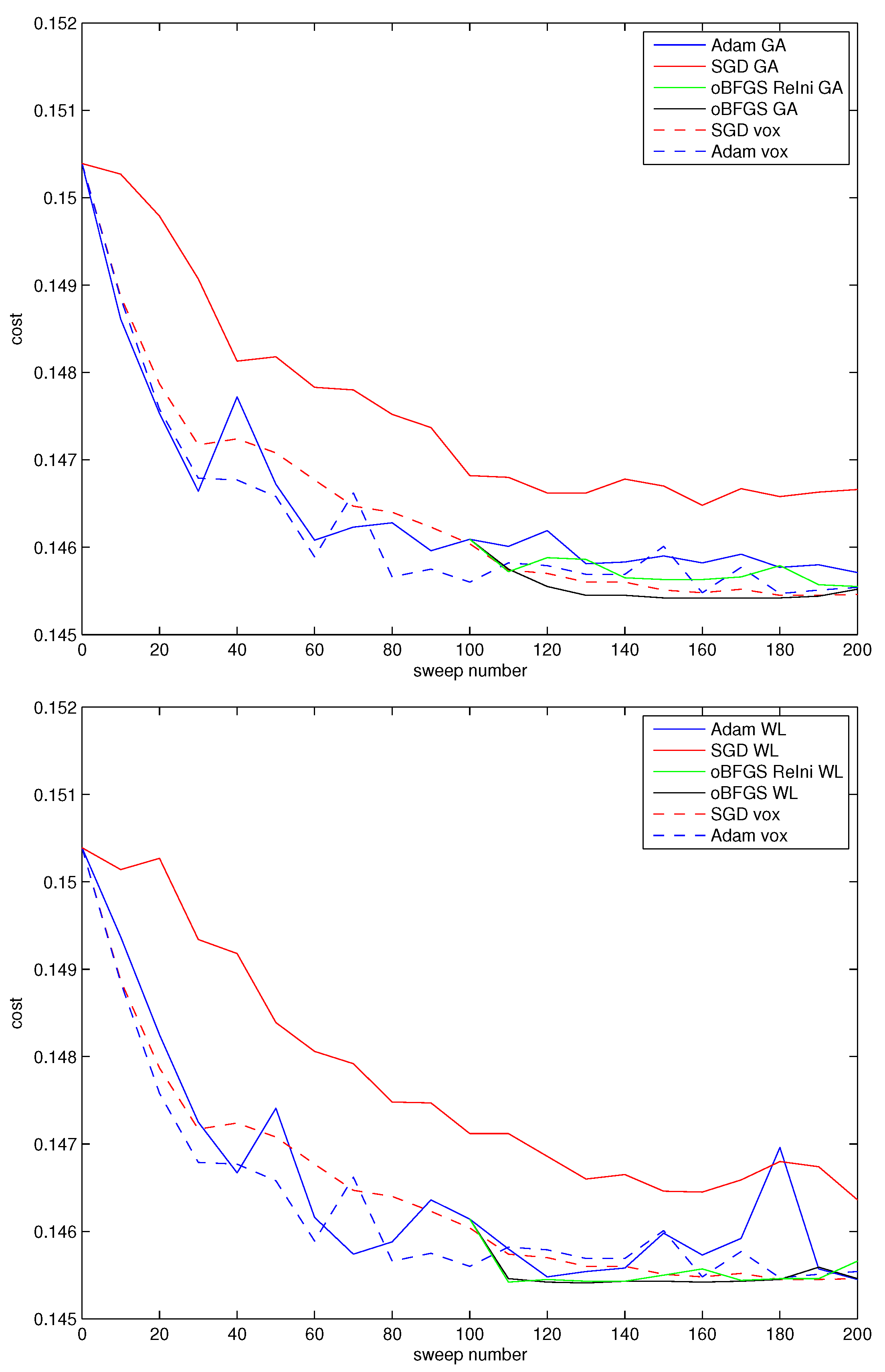
3. Results and Discussion

In this section, we provide details on the numerical evaluation of the algorithms as performed in our numerical experiments.

We recall that the ultimate goal is to determine an accurate estimation of location and size of targets of interest embedded within the domain in a fast and inexpensive fashion. This is realized by retrieving the permittivity profile starting from the measurements collected by the antennas. In the following, we assume that the building walls and the relative permittivity values of the objects are known while the shapes and locations of the targets are unknown. All algorithms are iteratively applied for a total number of sweeps equal to $N_{sweep}=200$. We assume also the following parameter values: $N_{cost}=10,N_{ReIni}=10,I_{vox}=[5,16]$.

In this section, we provide a comparison of the performance and of the algorithms described before, for both sets of basis functions (Gaussian and Wendland RBFs). We are, in particular, interested in the question of whether the final shape obtained is a good approximation to the true object location and size, and how fast a reasonable approximation is obtained in terms of iteration count. In addition to visual evaluation of the final reconstruction, we will also analyse the evolution of the data misfit cost as an indicator for efficiency of the algorithms. The shape evolution itself is not displayed here for the sake of brevity.

All numerical experiments are performed on a standard CPU workstation, which is sufficient for the computational setup considered here. For more complex situations, one might resort instead to GPU architectures as proposed in [38] which is likely to speed up all calculations accordingly. Currently, we do not expect that the overall comparison of stochastic optimization methods as reported in this paper will look significantly different on GPU architectures compared to the CPU system as used in our study. We plan to incorporate GPU processing in our future research for handling more complex 3D situations.

We start by discussing briefly the initial guess chosen as the starting point for the reconstructions. As illustrated in the right image of Figure 1, the initial guess consists of two different objects located at specific positions of the domain. One is closely located near the true position of the target, the other represents an artefact which is at an incorrect location. This choice of the initial guess can be shown to be a good approximation for practical applications in particular when a given time sequence is considered. In those applications, there is often a predicted location of the target in addition to some additional options which might be considered as well. Moreover, from a few iterations of a pixel-based scheme (which are usually fast to obtain) a similarly looking initial guess can be inferred quickly by some form of simple thresholding even without previous time steps available. The usual task is to improve on such a crude initial assumption quickly and to provide more reliable estimates on the actual shapes and sizes of objects. Usually those initial iterations of pixel-based schemes contain several of such ghost objects in addition to the first approximations of the true objects, due to the non-linear nature of the underlying inverse problem. The separation between ghosts and true objects cannot easily be obtained by pure pixel-based approaches. Our observation so far is that shape-based approaches perform better here. For more details on issues of the initial guess and a comparison of pixel versus shape-based approaches, we refer to [4,8] and references provided there.

The speed of convergence of the different schemes is highlighted here by considering the evolution of cost values against iteration count. We do not distinguish here between small differences in computational time per iteration for the three considered methods. Moreover, while the first-order techniques are applied here directly from the initial guess introduced above, the quasi-Newton methods are applied instead to the outcome of 100 sweeps of the Adam reconstruction. This choice has been made because quasi-Newton algorithms require a convex cost functional and, as anticipated, we attempt to satisfy this condition by considering its second-order Taylor approximation in proximity of a local minimum. The initial 100 iterations of the Adam method are included in the iteration count for the quasi-Newton methods. In general, a smaller number of initial Adam iterations can also be chosen for initializing the oBFGS scheme.

Figure 2 shows the evolution of the cost value with respect to the sweep number of the different constellations considered here. We observe the following. Adam performs better than SGD in the sense that it leads to a faster reduction of the cost value with both basis functions considered. Adam seems to have converged by the end of the simulation while this is not the case with SGD, especially when WL functions are used.

The effects of the introduction of a parametrization of the level set function are different for the two first-order methods considered. It leads to a slower descending trend with the SGD algorithm while it introduces a certain degree of instability with Adam, as shown by the irregular cost behaviour. This is reflected in the accuracy of the retrieved shapes as illustrated in the following.

The introduction of quasi-Newton schemes seems helpful. The use of oBFGS not only leads to the lowest value of the final cost, but also improves the stability of the reconstruction providing smoother trends than Adam. oBFGS performs better in absence of reinitialization procedure. This might be justified by the fact that, since we apply the quasi-Newton method starting from a configuration close to the true profile (i.e., minimum of the cost), the reinitialization of the (inverse) Hessian approximation leads to a loss of information accumulated in previous iterations.

The residual trends considered so far provide an overview of the evolution of the simulations. However, an exhaustive comparison of optimization algorithms requires to take into account also the final permittivity profiles achieved. The importance of this analysis is twofold. Firstly, it provides an effective visual comparison of the algorithms considered; secondly, it shows the effects of the parametrization in the shape representation.

Figure 3 shows that all algorithms are able to eliminate the artefact included in the initial guess and to identify the presence of an object in correspondence of the true target. However, the accuracy of the retrieved estimations is different. Among the GA parametrized techniques, oBFGS GA leads to the best result. However, all algorithms based on RBFs provide more irregular shapes than pixel-based level set methods. The good oBFGS final result justifies why the method corresponds to the lowest value of the cost value as discussed before.

Smoother boundaries in the parametric shape representations are achieved by WL RBFs as illustrated by Figure 4. Even though SGD WL contains an artefact, this class of basis function performs overall better than the previous one. In particular, the outcome of oBFGS WL is the closest to the true profile as shown in Figure 1.

The previous comparisons are made assuming the same fixed line search scheme. This scheme does not enforce a continuous reduction of the cost but requires, at each iteration, that the number of pixels which change their permittivity value is included in a given interval $I_{vox}$. The selection of the extreme values of this interval corresponds to the choice of the step sizes in traditional optimization algorithms. A trade-off is usually necessary. In fact, small step sizes lead to a stable evolution but might suffer from slow convergence in general. On the other hand, large amplitudes increase the speed of convergence but might produce instabilities. This choice is also critical in machine learning applications, where the value of the learning rate plays a major role.

In order to evaluate the sensitivity of the discussed optimization schemes to this crucial parameter, we have performed an additional set of simulations in which we increase the interval of permitted step sizes in the line search. To be precise, we have doubled the extreme values of $I_{vox}$. The corresponding cost evolution curves are displayed in Figure 5.

Although Figure 5 leads to general conclusions similar to our previous discussion, some differences emerge as well. For example, as a consequence of the extension of the interval $I_{vox}$, the shapes are allowed to change more significantly, yielding a rapid convergence especially at the beginning of the evolution. However, as expected, this also comes with some instabilities in the final part of the simulations as confirmed by the more irregular behaviours of the cost evolution compared to the trends depicted in Figure 2. Certainly, an adaptive selection of step sizes, e.g., being reduced with increasing iteration number, recommends itself here. Such an approach has been applied in a different application of low-frequency electromagnetic imaging in [26,27] with very good success. However, a similar more detailed study of adaptive line search techniques for the application in stochastic shape optimization schemes for through-the-wall radar imaging is beyond the scope of this paper.

4. Conclusions

In this work, we have analysed the performance of different stochastic optimization algorithms applied to solve a shape-based electromagnetic inverse problem. The goal is to retrieve targets of interest hidden behind walls. We investigated the capability of the parametric level set approach with different sets of radial basis functions for modelling the underlying stochastic shape evolution driven by the minimization of a given cost functional. The parametric level set approach reduces the dimensionality of the inverse problem and provides a tool for introducing some additional form of regularization into the inverse problem. It allows us to implement stochastic optimization methods that take into account information beyond the gradient direction, for example, stochastic quasi-Newton methods. In the numerical experiments provided, we observed that with this parametric representation of level sets, the hybrid approach combining Adam and oBFGS algorithms yielded both the lowest cost and best shape reconstructions. We also compared the parametrized level set approach with a more standard pixel-based representation of level set functions. We highlighted that the parametrization leads to more irregular boundaries compared to standard pixel-based representations; however, often achieving lower cost values and faster reconstructions. All algorithms considered have been equipped with the same inexpensive, flexible and efficient line search procedure. Finally, the robustness of the results with respect to details of this specific line search method has also been investigated in this paper.

References

1. Nkwari, P.K.M.; Sinha, S.; Ferreira, H.C. Through-the-wall radar imaging: A review. IETE Tech. Rev. 2018, 35, 631–639. [Google Scholar] [CrossRef]
2. Incorvaia, G.; Dorn, O. 2D Through-the-wall Radar Imaging Using a Level Set Approach. In Proceedings of the 2019 PhotonIcs & Electromagnetics Research Symposium-Spring (PIERS-Spring), Rome, Italy, 17–20 June 2019; pp. 63–72. [Google Scholar]
3. Dorn, O.; Miller, E.L.; Rappaport, C.M. A shape reconstruction method for electromagnetic tomography using adjoint fields and level sets. Inverse Probl. 2000, 16, 1119. [Google Scholar] [CrossRef]
4. Incorvaia, G.; Dorn, O. Tracking targets from indirect through-the-wall radar observations. In Proceedings of the 2020 14th European Conference on Antennas and Propagation (EuCAP), Copenhagen, Denmark, 15–20 March 2020; pp. 1–5. [Google Scholar]
5. Ampazis, N.; Perantonis, S.J. Two highly efficient second-order algorithms for training feedforward networks. IEEE Trans. Neural Netw. 2002, 13, 1064–1074. [Google Scholar] [CrossRef] [PubMed]
6. Shepherd, A.J. Second-Order Methods for Neural Networks: Fast and Reliable Training Methods for Multi-Layer Perceptrons; Springer: Berlin/Heidelberg, Germany, 2012. [Google Scholar]
7. Dorn, O.; Lesselier, D. Level set methods for inverse scattering. Inverse Probl. 2006, 22, R67. [Google Scholar] [CrossRef] [Green Version]
8. Dorn, O.; Miller, E.L.; Rappaport, C.M. Shape reconstruction in 2D from limited-view. In Radon Transforms and Tomography: 2000 AMS-IMS-SIAM Joint Summer Research Conference on Radon Transforms and Tomography, Mount Holyoke College, South Hadley, MA, USA, 18–22 June 2000; American Mathematical Society: Providence, RI, USA, 2001; Volume 278, p. 97. [Google Scholar]
9. Dorn, O.; Lesselier, D. Level set methods for inverse scattering - some recent developments. Inverse Probl. 2009, 25, 125001. [Google Scholar] [CrossRef]
10. Berenger, J.P. A perfectly matched layer for the absorption of electromagnetic waves. J. Comput. Phys. 1994, 114, 185–200. [Google Scholar] [CrossRef]
11. Osher, S.; Sethian, J. Fronts propagating with curvature-dependent speed: Algorithms based on Hamilton- Jacobi formulations. J. Comput. Phys 1988, 79, 12–49. [Google Scholar] [CrossRef] [Green Version]
12. Sethian, J. Level set Methods and Fast Marching Methods: Evolving Interfaces in Computational Geometry, Fluid Mechanics, Computers Visions and Material Sciences; Cambridge Monographs on Applied and Computational Mathematics; Cambridge University Press: Cambridge, UK, 1996. [Google Scholar]
13. Osher, S.; Fedkiw, R. Level set Method and Dynamic Implicit Surfaces. In Applied Mathematical Sciences; Springer: Berlin/Heidelberg, Germany, 2003; Volume 153. [Google Scholar]
14. Santosa, F. A Level-Set Approach for Inverse Problems Involving Obstacles. ESAIM Control. Optim. Calc. Var. 1996, 1, 17–33. [Google Scholar] [CrossRef]
15. Aghasi, A.; Kilmer, M.; Miller, E.L. Parametric level set methods for inverse problems. SIAM J. Imaging Sci. 2011, 4, 618–650. [Google Scholar] [CrossRef] [Green Version]
16. Kadu, A.; Van Leeuwen, T.; Mulder, W. A parametric level-set approach for seismic full-waveform inversion. In SEG Technical Program Expanded Abstracts 2016; Society of Exploration Geophysicists: Tulsa, OK, USA, 2016; pp. 1146–1150. [Google Scholar]
17. Larusson, F.; Fantini, S.; Miller, E.L. Parametric level set reconstruction methods for hyperspectral diffuse optical tomography. Biomed. Opt. Express 2012, 3, 1006–1024. [Google Scholar] [CrossRef] [Green Version]
18. Dorn, O.; Bertete-Aguirre, H.; Berryman, J.G.; Papanicolaou, G.C. A nonlinear inversion method for 3D electromagnetic imaging using adjoint fields. Inverse Probl. 1999, 15, 1523. [Google Scholar] [CrossRef]
19. Natterer, F.; Sielschott, H.; Dorn, O.; Dierkes, T.; Palamodov, V. Fréchet Derivatives for Some Bilinear Inverse Problems. SIAM J. Appl. Math. 2002, 62, 2092–2113. [Google Scholar] [CrossRef]
20. Wright, G.B. Radial Basis Function Interpolation: Numerical and Analytical Developments. Ph.D. Thesis, University of Colorado at Boulder, Boulder, CO, USA, 2003. [Google Scholar]
21. Zhang, T. Solving large scale linear prediction problems using stochastic gradient descent algorithms. In Twenty-First International Conference on Machine Learning; Association for Computing Machinery: New York, NY, USA, 2004; p. 116. [Google Scholar]
22. Johnson, R.; Zhang, T. Accelerating stochastic gradient descent using predictive variance reduction. Adv. Neural Inf. Process. Syst. 2013, 26, 315–323. [Google Scholar]
23. Hedges, L.O.; Kim, H.A.; Jack, R.L. Stochastic level-set method for shape optimisation. J. Comput. Phys. 2017, 348, 82–107. [Google Scholar] [CrossRef] [Green Version]
24. Wang, X.; Ma, S.; Goldfarb, D.; Liu, W. Stochastic quasi-Newton methods for nonconvex stochastic optimization. SIAM J. Optim. 2017, 27, 927–956. [Google Scholar] [CrossRef] [Green Version]
25. Dorn, O.; Hiles, A. A Level Set Method for Magnetic Induction Tomography of 3D Boxes and Containers. In Electromagnetic Non-Destructive Evaluation (XXI); IOS Press: Amsterdam, The Netherlands, 2018; pp. 33–40. [Google Scholar]
26. Hiles, A.; Dorn, O. Sparsity and level set regularization for near-field electromagnetic imaging in 3D. Inverse Probl. 2020, 36, 025012. [Google Scholar] [CrossRef]
27. Hiles, A.; Dorn, O. Colour level set regularization for the electromagnetic imaging of highly discontinuous parameters in 3D. Inverse Probl. Sci. Eng. 2020, 1–36. [Google Scholar] [CrossRef]
28. Bottou, L. Stochastic gradient learning in neural networks. Proc. Neuro-Nımes 1991, 91, 12. [Google Scholar]
29. Bottou, L. Large-scale machine learning with stochastic gradient descent. In Proceedings of COMPSTAT’2010; Springer: Berlin/Heidelberg, Germany, 2010; pp. 177–186. [Google Scholar]
30. Kingma, D.P.; Ba, J. Adam: A method for stochastic optimization. arXiv 2014, arXiv:1412.6980. [Google Scholar]
31. Schraudolph, N.N.; Yu, J.; Günter, S. A Stochastic Quasi-Newton Method for Online Convex Optimization. In Proceedings of the 11th International Conference on Artificial Intelligence and Statistics (AISTATS 2007); 2007; pp. 436–443. Available online: http://proceedings.mlr.press/v2/schraudolph07a/schraudolph07a.pdf (accessed on 29 September 2020).
32. Fletcher, R. A new approach to variable metric algorithms. Comput. J. 1970, 13, 317–322. [Google Scholar] [CrossRef] [Green Version]
33. Liu, D.C.; Nocedal, J. On the limited memory BFGS method for large scale optimization. Math. Program. 1989, 45, 503–528. [Google Scholar] [CrossRef] [Green Version]
34. Byrd, R.H.; Hansen, S.L.; Nocedal, J.; Singer, Y. A stochastic quasi-Newton method for large-scale optimization. SIAM J. Optim. 2016, 26, 1008–1031. [Google Scholar] [CrossRef]
35. Dai, Y.H.; Liao, L.Z.; Li, D. On restart procedures for the conjugate gradient method. Numer. Algorithms 2004, 35, 249–260. [Google Scholar] [CrossRef]
36. Powell, M.J.D. Restart procedures for the conjugate gradient method. Math. Program. 1977, 12, 241–254. [Google Scholar] [CrossRef]
37. Nocedal, J.; Wright, S. Numerical Optimization, 2nd ed.; Springer: Berlin/Heidelberg, Germany, 2006. [Google Scholar]
38. Breglia, A.; Capozzoli, A.; Curcio, C.; Liseno, A. CUDA expression templates forelectromagnetic applications on GPUs. IEEE Antennas Prop. Mag. 2013, 55, 156–166. [Google Scholar] [CrossRef]
Figure 1. To the (left): example setup considered. To the (right): initial guess adopted in the simulations.
Electronics 09 02055 g001
Figure 2. Cost versus sweep number. Top image: Gaussian Radial Basis Functions (RBF); Bottom image: Wendland RBF. The blue, red, green and black curves refer, respectively, to the following algorithms: Adam, SGD, oBFGS with reinitialization every N R e I n i = 10 sweeps and oBFGS (without reinitialization). The dashed lines correspond to level set pixel-based Adam and Stochastic Gradient Descent (SGD) reconstructions.
Electronics 09 02055 g002
Figure 3. Final permittivity profiles achieved. Top row from left to right: SGD GA, Adam GA and SGD vox. Bottom row from left to right: oBFGS GA, oBFGS ReIni GA, Adam vox.
Electronics 09 02055 g003
Figure 4. Final permittivity profiles achieved. Top row from left to right: SGD WL, Adam WL and SGD vox. Bottom row from left to right: oBFGS WL, oBFGS ReIni WL, Adam vox.
Electronics 09 02055 g004
Figure 5. Cost versus sweep number doubling the extreme values of I v o x . Top image: Gaussian RBF; Bottom image: Wendland RBF. The blue, red, green and black curves refer, respectively, to the following algorithms: Adam, SGD, oBFGS with reinitialization every N R e I n i = 10 sweeps and oBFGS (without reinitialization). The dashed lines correspond to level set pixel-based Adam and SGD reconstructions.
Electronics 09 02055 g005
Publisher’s Note: MDPI stays neutral with regard to jurisdictional claims in published maps and institutional affiliations.