Multi-Step Learning-by-Examples Strategy for Real-Time Brain Stroke Microwave Scattering Data Inversion

Abstract

This work deals with the computationally-efficient inversion of microwave scattering data for brain stroke detection and monitoring. The proposed multi-step approach is based on the Learning-by-Examples (LBE) paradigm and naturally matches the stages and time constraints of an effective clinical diagnosis. Stroke detection, identification, and localization are solved with real-time performance through support vector machines (SVMs) operating both in binary/multi-class classification and in regression modalities. Experimental results dealing with the inversion of laboratory-controlled data are shown to verify the effectiveness of the proposed multi-step LBE methodology and prove its suitability as a viable alternative/support to standard medical diagnostic methods.

1. Introduction

The use of microwave radiation for sensing the human body is an emerging technology and a promising alternative/support to well-established medical equipment, such as magnetic resonance imaging ($MRI$ ) and computed tomography ($CT$) [1,2,3]. As a matter of fact, differently from $MRI$ and $CT$, microwave imaging ($MI$) takes advantage of desirable features, such as lower costs, easier deployment (since it does not require the patient to be transported to an appropriately equipped hospital), and faster acquisition times, as well as the use of non-ionizing radiation [2]. For such reasons, it is currently attracting many researchers, being a promising candidate for many medical applications requiring a continuous monitoring/treatment, as in the case of brain strokes [4,5,6,7,8,9,10,11]. Within this context, strokes are, worldwide, the third leading cause of death and the first one of neurological dysfunction, with an estimated annual expense for patients treatment of 64.1 billion in Europe only [12]. The probability of permanent consequences of a stroke are strongly related to the amount of time that passes from the first symptoms/its detection to the early treatment. Moreover, the identification of the type of stroke, besides its localization, plays a critical role in the decision of the most appropriate intervention [4,5]. As an example, thrombolytic treatment can be disastrous if applied to a patient with an hemorrhagic stroke (i.e., caused by bleeding), rather than an ischaemic one (i.e., caused by the obstruction of a blood vessel) [13].

Several studies have been recently published on brain stroke $MI$. To cite a few representative examples, the Born Iterative Method ($BIM$) has been successfully applied in Reference [7] for retrieving $2D$ guesses of brain tissues from numerical data. However, the time required for a single reconstruction (i.e., approximately 4 h [7]) is not compatible with a real-time monitoring. The exploitation of modern graphics processing units ($GPU$s) and parallel computing has been recently explored [4,5] to reduce the inversion time, but unfortunately such solutions still appear to be clinically unfeasible for the continuous monitoring of the patient’s head. Alongside such promising advancements, Learning-by-Examples ($LBE$) methods are rapidly emerging as a viable alternative towards real-time performance [14,15,16,17,18,19,20,21,22,23,24,25]. As a matter of fact, they do not require the solution of any forward scattering equation to produce a diagnosis, the computational load/complexity being shifted to the off-line generation of a fast prediction model from a suitable set of known input/output ($I/O$) pairs [14]. Within this context, this work has the objective to present a new multi-step $LBE$ strategy that naturally fits the clinical need of multi-level information about the patient’s health status. More specifically, the inversion of experimental $MI$ data is addressed in a computationally efficient way to progressively (i) detect the presence of a stroke, (ii) identifying its typology, and, finally, (iii) localizing it. Such steps are accomplished through support vector machines ($SVM$)-based inversion algorithms exploiting binary/multi-class classification and regression formulations. The SVM framework has been adopted in this work because of several positive features, including (i) a solid mathematical background, (ii) the absence of local minima during the training phase, (iii) its intrinsic capability to deal with noisy (i.e., real-world) acquisitions, (iv) the high computational efficiency, and (v) the availability of both classification and regression formulations [26].

It is worth highlighting that the main contribution of this work over the existing literature and preliminary validations from the authors [22,23] consists in the following key aspects: (i) an innovative integrated multi-step diagnosis framework exploiting progressively acquired information on the monitored patient’s health status, (ii) a novel regression-based localization approach to yield accurate predictions of the location of a previously-detected brain stroke, (iii) practical guidelines on the setting of the main SVM parameters, as well as (iv) insights on the nature/behavior of real scattering data acquired in a controlled environment when dealing with both ischaemic and hemorrhagic stroke phantoms. The paper is organized as follows. Section 2 describes the mathematical formulation of the problem and the proposed multi-step $LBE$-based inversion strategy. Some representative experimental results are reported in Section 3 to assess the effectiveness of the proposed method. Finally, some concluding observations and remarks are drawn (Section 4).

2. Multi-Step $\mathit{LBE}$ Brain Stroke Diagnosis

With reference to the geometry sketch in Figure 1, let us model the human brain as an investigation domain $\mathcal{D}\in {\mathbb{R}}^3$ made of an inhomogeneous, lossy, and non-magnetic medium [4].

A set of V antennas working at central frequency $f_0$ and placed over an external observation domain ${\mathcal{D}}_{obs}$ is exploited to sense $\mathcal{D}$ through electromagnetic (EM) waves and retrieve information on its status (Figure 1). Accordingly, under the v-th illumination ($v=1,\dots ,V$), the scattering phenomena occurring between incident wave and probed scenario [4] are measured in ${\mathcal{D}}_{obs}$ as the ensemble of V complex scattering coefficients

$${\tilde{S}}_{uv}=\frac{{\tilde{\psi }}_u^{-}}{{\tilde{\psi }}_v^{+}}=S_{uv}^{\Re }+j{S}_{uv}^{\Im };u=1,\dots ,V,$$

(1)

with ${\tilde{\psi }}_u^{-}$ and ${\tilde{\psi }}_v^{+}$ denoting the reflected and incident voltages at the u-th and v-th antennas, respectively. From an EM point of view, the presence in $\mathcal{D}$ of a stroke is modeled as a volumetric region $\mathsf{\Omega }\subset \mathcal{D}$ with complex permittivity ${\tilde{\epsilon }}^S$ different from the average properties of the surrounding medium (i.e., healthy brain tissue, ${\tilde{\epsilon }}^B={\epsilon }^B-j\frac{{\sigma }^B}{2\pi f}$—Figure 1) (It is worth remarking that, according to the reference literature [27], the considered conductivity model is a dispersive one, which has been sampled at the central frequency of the measurement equipment.). Moreover, it is worth observing that ${\tilde{\epsilon }}^S$ is proportional to the amount of blood inside $\mathsf{\Omega }$: indicating, with ${\tilde{\epsilon }}_{\mathcal{H}/\mathcal{I}}^S={\epsilon }_{\mathcal{H}/\mathcal{I}}^S-j\frac{{\sigma }_{\mathcal{H}/\mathcal{I}}^S}{2\pi f}$, the permittivity of an hemorrhagic/ischaemic stroke, it is typically verified that ${\epsilon }_{\mathcal{H}}^S>{\epsilon }^B>{\epsilon }_{\mathcal{I}}^S$ and ${\sigma }_{\mathcal{H}}^S>{\sigma }^B>{\sigma }_{\mathcal{I}}^S$ [4]. Obtaining a reliable diagnosis of $\mathcal{D}$ starting from the acquired data in ${\mathcal{D}}_{obs}$ can be decomposed as a three-step process, in which each stage is aimed at gradually increasing the level of information on the monitored domain, and solved through a dedicated $LBE$ strategy, as detailed in the following Sections.

2.1. Step 1—“Detection”

The first step, necessary to trigger successive deeper diagnoses, is that of detecting the presence of a stroke within the monitored patient’s head. Towards this goal, the $LBE$ inversion of scattered data is formulated as a binary classification problem. Accordingly, a $SVM$ classifier is trained on a set of N known $I/O$ pairs

$$\mathsf{\Psi }=\left\{\left[{\mathbf{\xi }}_n;\mathcal{L}\left({\mathbf{\xi }}_n\right)\right];n=1,\dots ,N\right\},$$

(2)

where

$${\mathbf{\xi }}_n=\left\{\left(S_{uv,n}^{\Re },S_{uv,n}^{\Im }\right);u,v=1,\dots ,V;u\le v\right\}$$

(3)

contains the $\left(V+1\right)\times V$ measured features (It should be pointed out that any pre-processing nor cleaning operation (e.g., averaging/filtering) has been performed on the measured data, except the fact that only the upper-part of the scattering matrix has been exploited by enforcing ${\tilde{S}}_{uv}={\tilde{S}}_{vu}$.), while $\mathcal{L}\left({\mathbf{\xi }}_n\right)$ is the corresponding label indicating the presence (i.e., $\mathcal{L}\left({\mathbf{\xi }}_n\right)=+1$) or absence (i.e., $\mathcal{L}\left({\mathbf{\xi }}_n\right)=-1$) of a stroke inside $\mathcal{D}$.

Starting from the information in $\mathsf{\Psi }$ a fast detector is then built solving—through the Sequential Minimal Optimization ($SMO$) algorithm [26]—the following quadratic problem:

$$\begin{array}{cc}\underset{\mathbf{\alpha }}{min}\hfill & \frac{1}{2}{\mathbf{\alpha }}^T\mathbf{Q}\mathbf{\alpha }-{\mathbf{1}}^T\mathbf{\alpha }\hfill \\ \mathrm{subject}\mathrm{to}\hfill & {\mathcal{L}}^T\mathbf{\alpha }=0\hfill \end{array}$$

(4)

where $\mathbf{\alpha }={\left\{\left(0\le {\alpha }_n\le C\right);n=1,\dots ,N\right\}}^T$, C being a regularization parameter, $\mathcal{L}={\left\{\mathcal{L}\left({\mathbf{\xi }}_n\right);n=1,\dots ,N\right\}}^T$, $\mathbf{Q}$ is an $N\times N$ matrix with $mn$-th entry $Q_{mn}=\mathcal{L}\left({\mathbf{\xi }}_m\right)\mathcal{L}\left({\mathbf{\xi }}_n\right)$$exp\left(-\gamma {∥{\mathbf{\xi }}_m-{\mathbf{\xi }}_n∥}^2\right)$, $m,n=1,\dots ,N$, $\mathbf{1}={\left[1,\dots ,1\right]}^T$, $\gamma$ is a user-defined parameter, and ${.}^T$ is the transpose operator. Finally, a diagnosis is immediately obtained during the on-line phase, starting from a new measurement $\mathbf{\xi }$ as

$$\widehat{\mathcal{L}}\left(\mathbf{\xi }\right)=\mathrm{sgn}\left(\sum _{n=1}^N\mathcal{L}\left({\mathbf{\xi }}_n\right){\alpha }_{n}exp\left(-\gamma {∥{\mathbf{\xi }}_n-\mathbf{\xi }∥}^2\right)+b\right),$$

(5)

where b is computed exploiting the Karush-Kuhn-Tucker ($KKT$) conditions [26].

2.2. Step 2—“Identification”

In those cases where the outcome of Step 1 is positive (i.e., a stroke has been detected), an immediate feedback to the medical staff is required to determine the type of pathology and suggest the proper treatment. Accordingly, the goal of the second $LBE$ step is to discriminate between the ischaemic or hemorrhagic nature of the detected stroke. The problem is again formulated as a binary classification one and solved in the same manner as the first step, under an updated assignment of the physical meaning of training labels: $\mathcal{L}\left({\mathbf{\xi }}_n\right)=-1$ for ischaemic and $\mathcal{L}\left({\mathbf{\xi }}_n\right)=+1$ for hemorrhagic, respectively, ($n=1,\dots ,N$).

2.3. Step 3—“Localization”

Once the brain stroke has been detected (Step 1—“Detection”) and classified (Step 2—“Identification”), a further step to complete the $LBE$ diagnosis and provide a quick feedback to the medical staff is that of retrieving a guess of the stroke position, ${\mathbf{r}}^S=\left(x^S,y^S,z^S\right)$ (Figure 1). Towards this end, the inversion of scattering data can be addressed through a dedicated (a) multi-class classification and/or (b) regression strategy.

Following the solution approach (a), the estimation process is aimed at identifying the most probable position of the pathology within a predefined set of P candidate locations ${\mathbf{r}}_p\in \mathcal{D}$, $p=1,\dots ,P$ (Figure 1). Accordingly, a direct position/class correspondence is considered, by letting

$$\mathcal{L}\left({\mathbf{\xi }}_n\right)\in \left\{p=1,\dots ,P\right\};n=1,\dots ,N.$$

(6)

The one-against-one strategy is adopted by building $\frac{P\times \left(P-1\right)}{2}$ binary $SVM$ classifiers, each one trained on scattering data from only two classes [28]. A voting strategy is then applied to identify the most probable stroke position, designating it as the p-th class with the maximum number of “votes” among all trained $SVM$ models.

Alternatively, according to (b), the estimation of the stroke coordinates,

$${\zeta }^S\in \left\{x^S,y^S,z^S\right\},$$

(7)

is achieved through a support vector regression ($SVR$) strategy by solving the following quadratic problem

$$\begin{array}{c}\underset{\mathbf{\beta },{\mathbf{\beta }}^{*}}{min}\frac{1}{2}{\left(\mathbf{\beta }-{\mathbf{\beta }}^{*}\right)}^T\mathbf{W}\left(\mathbf{\beta }-{\mathbf{\beta }}^{*}\right)+ϵ\sum _{n=1}^N\left({\beta }_n+{\beta }_n^{*}\right)+\sum _{n=1}^N{\zeta }_n^S\left({\beta }_n-{\beta }_n^{*}\right)\hfill \\ \\ \mathrm{subject}\mathrm{to}{\mathbf{e}}^T\left(\mathbf{\beta }-{\mathbf{\beta }}^{*}\right)=0,\hfill \end{array}$$

(8)

where $ϵ>0$ defines the insensitive tube [14], and the $mn$-th entry of $\mathbf{W}$ is

$$W_{mn}=exp\left(-\delta {∥{\mathbf{\xi }}_m-{\mathbf{\xi }}_n∥}^2\right);m,n=1,\dots ,N,$$

(9)

and

$$\mathbf{\beta },{\mathbf{\beta }}^{*}={\left\{\left(0\le {\beta }_n,{\beta }_n^{*}\le A\right);n=1,\dots ,N\right\}}^T,$$

(10)

with A and $\delta$ being user-controlled parameters. Finally, ${\zeta }^S$ is predicted as

$${\widehat{\zeta }}_n^S\left(\mathbf{\xi }\right)=\sum _{n=1}^N\left({\beta }_n^{*}-{\beta }_n\right)exp\left(-\delta {∥{\mathbf{\xi }}_n-\mathbf{\xi }∥}^2\right)+h,$$

(11)

with h being a bias satisfying the $KKT$ conditions [26].

3. Experimental Validation

To assess the effectiveness and the potentialities of the proposed multi-step $LBE$ strategy, an experimental validation against laboratory-controlled data has been undertaken, as described in the following.

In all reported results, an average testing time of $\mathsf{\Delta }{t}^{test}=5\times {10}^{-3}$ s has been recorded using a standard laptop equipped with 8 GB RAM memory. Moreover, the computational resources required to train the different models have been always very limited and almost independent on the considered stage of the proposed multi-step approach, with training times always $\mathsf{\Delta }{t}^{train}\le 5$ s, whatever the considered training size.

3.1. Acquisition Set-Up and Experimental Data Analysis

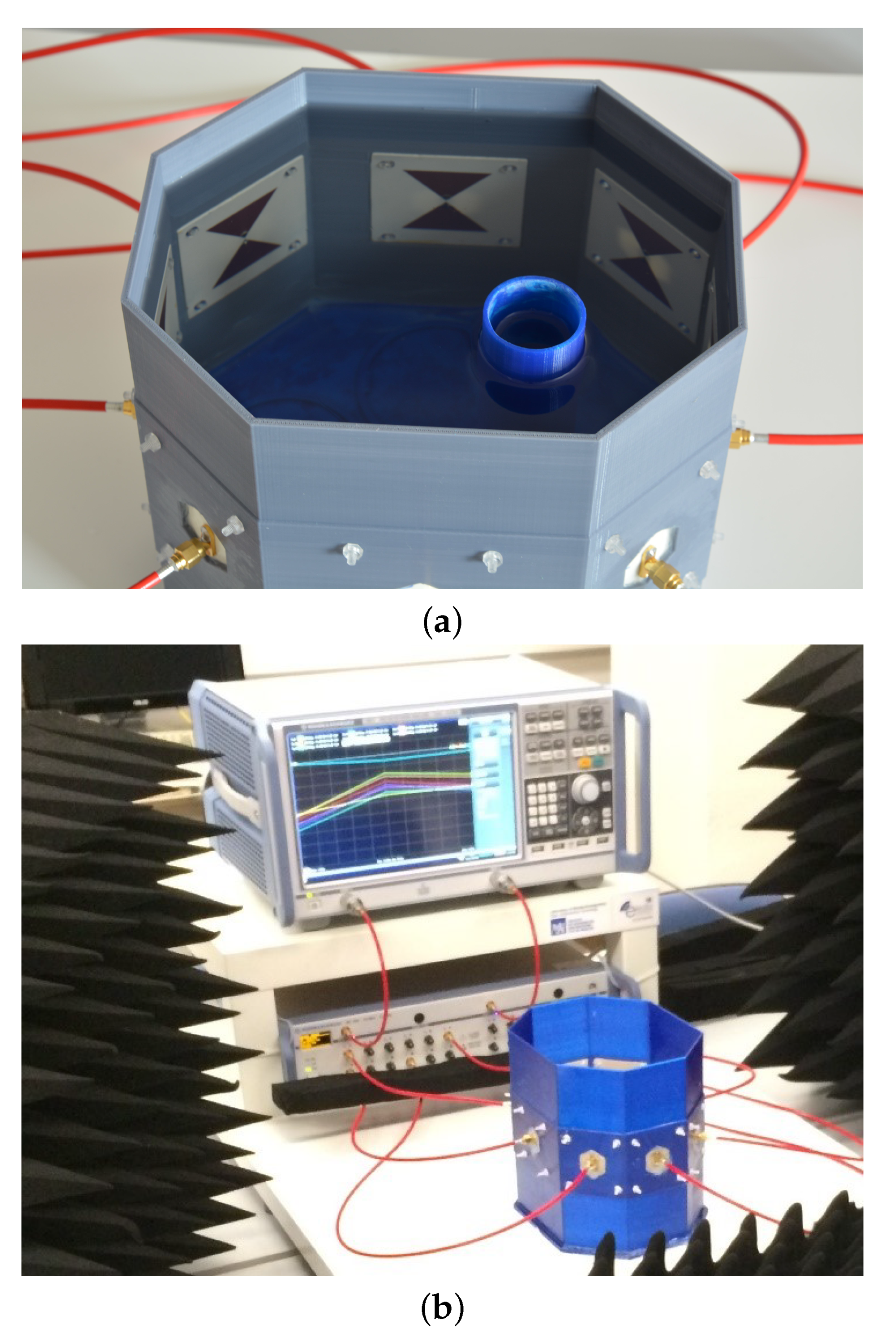
The experimental set-up has been designed and fabricated via $3D$ printing technology (Figure 2). It consisted of an octagonal prism sized $\left(L_1,L_2,L_3\right)=\left(200,160,200\right)$ mm modeling $\mathcal{D}$ (Figure 3), which has been filled by a liquid mixture yielding ${\epsilon }^B=41.8{\epsilon }_0$ and ${\sigma }^B=0.97$ S/m at 20 °C and $f_0=900$ MHz [29]. The is chaemic and hemorrhagic stroke phantoms have been realized with circular cylinders having diameter $d^S=40$ mm, height $h^S=200$ mm (Figure 3a), and filled with liquid mixtures providing ${\tilde{\epsilon }}_{\mathcal{I}}^S=32.04{\epsilon }_0-j\frac{0.85}{2\pi f_0}$ and ${\tilde{\epsilon }}_{\mathcal{H}}^S=48.63{\epsilon }_0-j\frac{1.28}{2\pi f_0}$, respectively.

Moreover, $V=8$ bow-tie antennas printed over Rogers Duroid 4003C substrate of thickness $1.5$ mm have been installed on each face of the prism at constant height (i.e., 100 mm) to form a $2D$ observation domain ${\mathcal{D}}_{obs}$ (Figure 2 and Figure 3). A microwave switching matrix R&S ZN-Z84 and a vector network analyzer R&S ZNB4 have been exploited to drive the acquisition process. As for the latter, the measurement of the full scattering matrix for a given configuration has been performed in about two seconds, thanks to a completely automated process, while moving the stroke phantom to a new position was done manually (due to the early stage of the prototype) in about one minute.

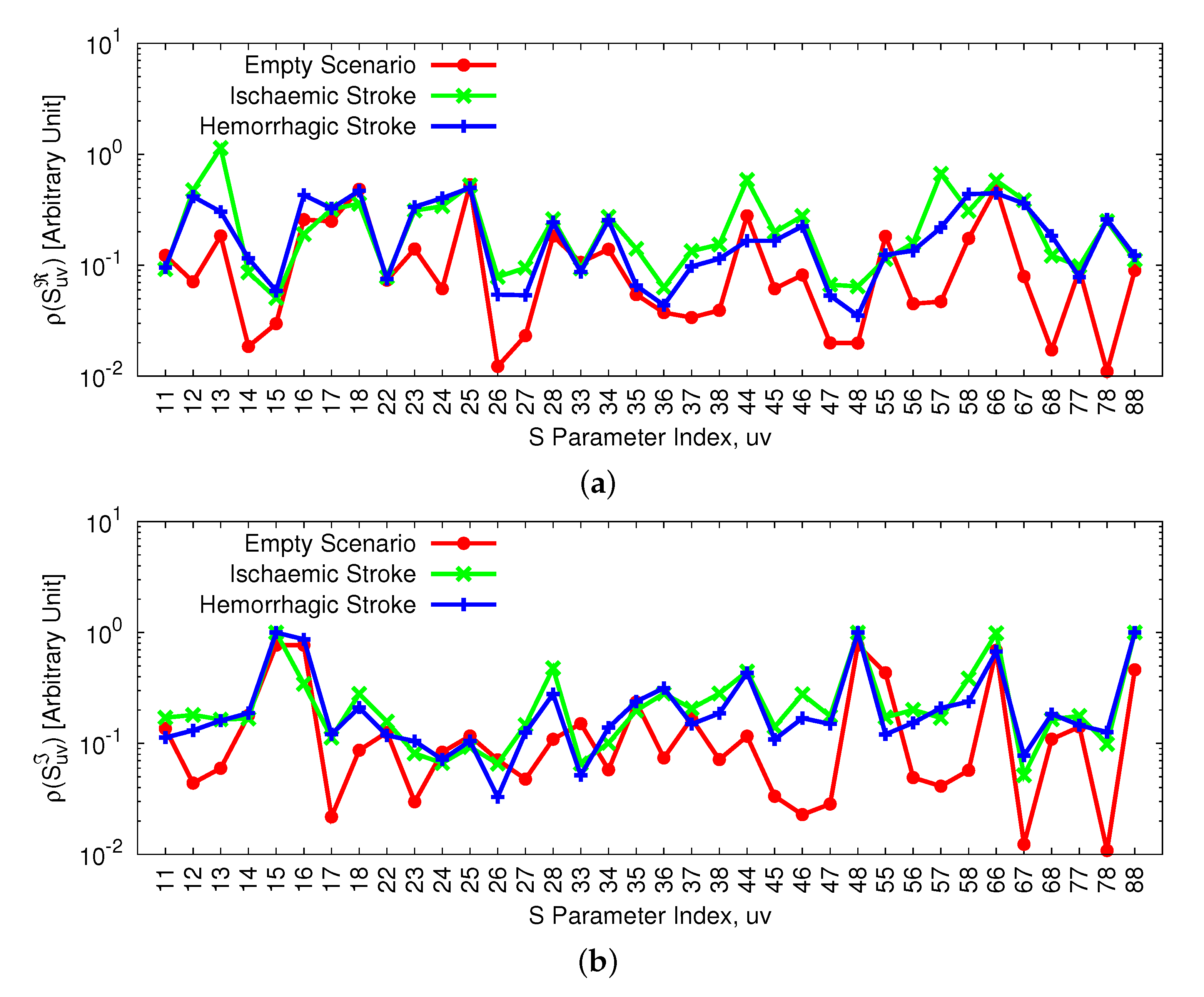
To have a better understanding of the acquired data, Figure 4 reports the coefficient of variation [30]

$$\rho \left(\chi \right)=\left(\sqrt{\frac{1}{K}\sum _{k=1}^K{\left({\chi }_k-\overline{\chi }\right)}^2}\right)/\overline{\chi },$$

(12)

where

$$\overline{\chi }=\frac{1}{K}\sum _{k=1}^K{\chi }_k,$$

(13)

computed over $K=1000$ acquisitions performed at three different day times (i.e., morning, afternoon, and evening), for both the real (i.e., $\chi =S_{uv}^{\Re }$, $u,v=1,\dots ,V$, $u\le v$; Figure 4a) and the imaginary (i.e., $\chi =S_{uv}^{\Im }$, $u,v=1,\dots ,V$, $u\le v$; Figure 4b) parts of the scattering coefficients. As it can be observed, larger data fluctuations are generated when a stroke is present inside the head phantom with respect to the “empty” case (Figure 4). At the same time, it is worth noticing that similar variations characterize the two stroke types, suggesting that the second step (i.e., “Identification”) may be a more difficult task with respect to the preliminary one (i.e., “Detection”). Furthermore, it is interesting to observe that larger, in general, occur between the three curves in correspondence to the transmission coefficients (i.e., $S_{uv}$, $u\ne v$), rather than the reflection ones (i.e., $S_{uv}$, $u=v$), suggesting that these latter probably carry less information about the status of $\mathcal{D}$ (Figure 4).

Finally, a statistical analysis has been performed on the measured scattering coefficients for both ischaemic (Figure 5a) and hemorrhagic (Figure 5b) strokes. As it can be observed from the plot of the minimum, maximum, and average values for both considered scenarios (Figure 5), there are fluctuations in the measurements acquired at different hours.

Such an outcome can be at least partially motivated by the natural deviations of the electromagnetic properties of the involved liquid mixtures due to a change of the surrounding environment (i.e., the temperature). Such an intrinsic variability has been exploited to enhance the robustness of the LBE algorithms by exploiting during the training phase measurements randomly chosen from the three data-sets. The same operation has been performed to build the test data, as well, in order to test the generalization capabilities of the trained models.

3.2. Inversion Results

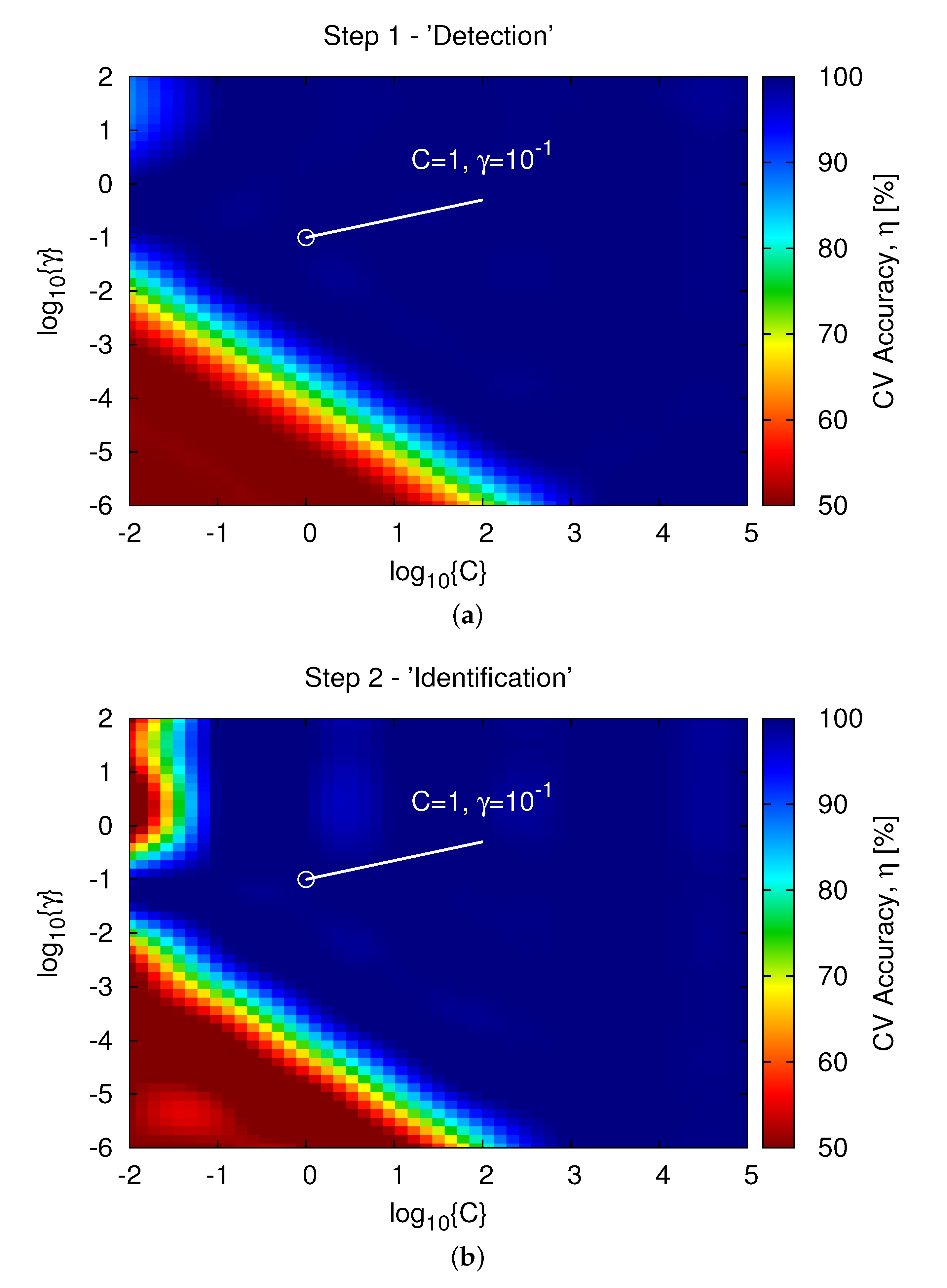
Dealing with Step 1 (“Detection”), training sets of increasing size N have been generated by collecting data equally distributed between “empty” (i.e., $\mathcal{L}\left({\mathbf{\xi }}_n\right)=-1$—no stroke is present in $\mathcal{D}$) and “full” (i.e., $\mathcal{L}\left({\mathbf{\xi }}_n\right)=+1$—a stroke is present in $\mathcal{D}$) scenarios, randomly varying both position and type of stroke for the latter class. A careful tuning has been performed for selecting the optimal $SVM$ control parameters C and $\gamma$ through a 5-fold cross-validation ($CV$) strategy [22].

Figure 6a shows the outcome of such a calibration, indicating that a high $CV$ accuracy (i.e., $\eta >90\%$) is yielded over a large portion of the explored $\left(C,\gamma \right)$ space. Accordingly, in the following the inversion results have been obtained by letting $C=1$ and $\gamma ={10}^{-1}$. Moving the focus towards the on-line capabilities of the trained detector, Figure 7a shows the actual versus predicted labels when processing $M=500$ previously-unseen measurements with $N=10$ training samples. As it can be observed, such a training configuration is insufficient for obtaining reliable diagnoses, as verified by the high percentage of false positives (i.e., ${\Xi }_{-1\to +1}^{N=10}=24.4$%—Figure 7a). On the other hand, it should be noticed that only $N=50$ training samples are sufficient to completely avoid wrong detections (i.e., ${\Xi }_{-1\to +1}^{N=50}=0$%—Figure 7b).

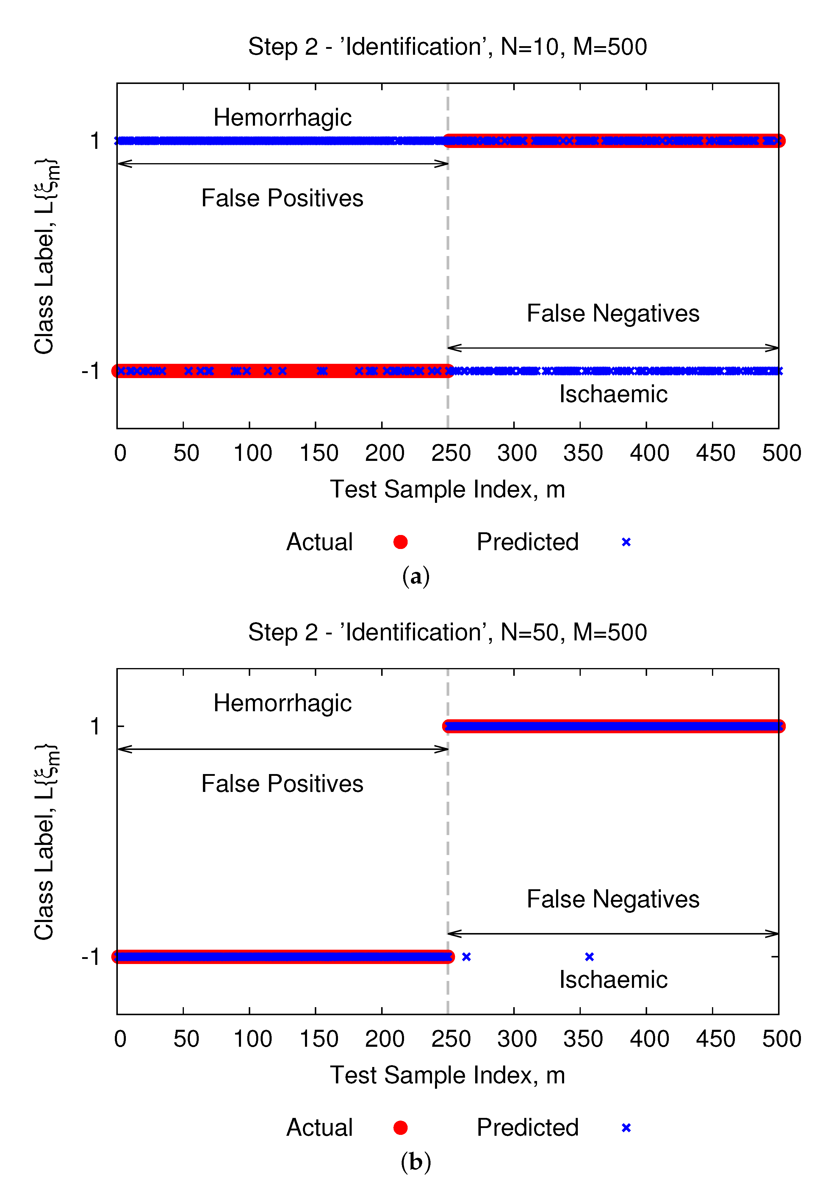
Moving to the Step 2 (“Identification”), the training set has been generated by considering an equal subdivision of samples for both ischaemic and hemorrhagic cases. Almost the same behavior characterizes the $CV$ error, suggesting again a robust and non-unique choice of the $\left(C,\gamma \right)$ parameters to achieve a high prediction accuracy (Figure 6b). Keeping the same optimal setting of the first step, the inversion outcomes confirm that this second task is slightly more difficult than the first one. As a matter of fact, the percentage of false positives and negatives with $N=10$ samples turns out to be almost unacceptable, being respectively equal to ${\Xi }_{-1\to +1}^{N=10}=85.6$% and ${\Xi }_{+1\to -1}^{N=10}=52.8$% (Figure 8a). Nevertheless, increasing the training size up to $N=50$ leads to an almost perfect discrimination between the two classes, with ${\Xi }_{-1\to +1}^{N=50}=0$% and ${\Xi }_{+1\to -1}^{N=50}=0.8$% (Figure 8b).

Finally, let us consider the third stage of the brain stroke diagnosis process (Step 3—“Localization”). Figure 9 summarizes the outcomes for the multi-class $SVM$ strategy, showing the predicted versus actual classes when considering $P=25$ partially-overlapped stroke positions (

Table 1. Experimental Assessment. ($V=8$, $f_0=900$ MHz, ${\tilde{\epsilon }}^B=41.8{\epsilon }_0-j\frac{0.97}{2\pi f_0}$, ${\tilde{\epsilon }}_{\mathcal{I}}^S=32.04{\epsilon }_0-j\frac{0.85}{2\pi f_0}$, ${\tilde{\epsilon }}_{\mathcal{H}}^S=48.63{\epsilon }_0-j\frac{1.28}{2\pi f_0}$)—Coordinates of the P candidate stroke locations within the imaged head phantom.

Position, p	$\left({\mathit{x}}_{\mathit{p}}^{\mathit{S}},{\mathit{y}}_{\mathit{p}}^{\mathit{S}}\right)$ [mm]	Position, p	$\left({\mathit{x}}_{\mathit{p}}^{\mathit{S}},{\mathit{y}}_{\mathit{p}}^{\mathit{S}}\right)$ [mm]
1	$\left(71,0\right)$	14	$\left(27,54\right)$
2	$\left(72,-27\right)$	15	$\left(58,46\right)$
3	$\left(58,-46\right)$	16	$\left(72,27\right)$
4	$\left(27,-54\right)$	17	$\left(35.5,0\right)$
5	$\left(0,-54\right)$	18	$\left(28,-27\right)$
6	$\left(-27,-54\right)$	19	$\left(0,-27\right)$
7	$\left(-58,-46\right)$	20	$\left(-28,-27\right)$
8	$\left(-72,-27\right)$	21	$\left(-35.5,0\right)$
9	$\left(-71,0\right)$	22	$\left(-28,27\right)$
10	$\left(-72,27\right)$	23	$\left(0,27\right)$
11	$\left(-58,46\right)$	24	$\left(28,27\right)$
12	$\left(-27,54\right)$	25	$\left(0,0\right)$
13	$\left(-0,54\right)$	-	-

) covering the whole cross-section of $\mathcal{D}$ (letting $C=1$ and $\gamma =1$, as indicated by a preliminary $CV$, and neglecting the z-coordinate, as dictated by the considered experimental set-up geometry).

As expected, given the higher complexity of the classification problem at hand and the lower separability between data, in this case, $N=50$ training samples (i.e., $N_p=2$ samples for each class/position, $p=1,\dots ,P$) are not sufficient for yielding faithful guesses of the stroke location (Figure 9a). Such a result is confirmed by the low percentage of correctly classified samples, which turns out to be equal to ${\mathsf{\Phi }}^{N=50}=6.6\%$ over $M=500$ test samples (

Table 2. Experimental Assessment. ($V=8$, $f_0=900$ MHz, ${\tilde{\epsilon }}^B=41.8{\epsilon }_0-j\frac{0.97}{2\pi f_0}$, ${\tilde{\epsilon }}_{\mathcal{I}}^S=32.04{\epsilon }_0-j\frac{0.85}{2\pi f_0}$, ${\tilde{\epsilon }}_{\mathcal{H}}^S=48.63{\epsilon }_0-j\frac{1.28}{2\pi f_0}$, $M=500$, $P=25$)—Error indexes vs. training size when solving Step 3 (“Localization”) through multi-class $SVM$ and $SVR$ approaches.

Training Size	Multi-Class $\mathit{SVM}$	Regression $\mathit{SVR}$
N	$\mathbf{\Phi }$ [%]	$\mathit{NME}\left({\mathit{x}}^{\mathit{S}}\right)$ [mm]	$\mathit{NME}\left({\mathit{y}}^{\mathit{S}}\right)$ [mm]
50	$6.6$	$3.61\times {10}^{-1}$	$3.27\times {10}^{-1}$
100	$13.8$	$1.67\times {10}^{-1}$	$1.46\times {10}^{-1}$
250	$84.6$	$4.05\times {10}^{-2}$	$2.99\times {10}^{-2}$
400	$96.6$	$1.31\times {10}^{-2}$	$7.91\times {10}^{-3}$

).

As a matter of fact, more samples are required to achieve good predictions, the accuracy increasing to ${\mathsf{\Phi }}^{N=400}=96.6\%$ for $N=400$ samples (i.e., $N_p=8$ samples for each class; Figure 9b and Table 2). Nevertheless, it is important to observe that the ratio between the the number of training samples, N, and the dimension of the input space for the SVM inversion (i.e., the number of measured features, $Q=\left(V+1\right)\times V=72$) is always very limited and lower than ${\left.\frac{N}{Q}\right|}_{N=400}=5.6$. Such an outcome confirms the good prediction accuracy of the method, even if a quite limited number of training samples has been used to train the model.

Similar outcomes are observed for the $SVR$-based solution, as indicated by the scatter plots of the actual versus predicted x-coordinate (i.e., $x^S$ vs. $\widehat{x^S}$; Figure 10a,c) and y-coordinate (i.e., $y^S$ vs. $\widehat{y^S}$; Figure 10b,d) of the stroke (letting $A={10}^4$ and $\delta =ϵ={10}^{-1}$). In this case, the normalized mean error (defined as in Reference [24]) is reduced by $\frac{{\left.NME\left(x^S\right)\right|}^{N=400}}{{\left.NME\left(x^S\right)\right|}^{N=50}}=3.63\times {10}^{-2}$ and $\frac{{\left.NME\left(y^S\right)\right|}^{N=400}}{{\left.NME\left(y^S\right)\right|}^{N=50}}=2.42\times {10}^{-2}$, respectively, when passing from $N=50$ to $N=400$ training samples (Table 2).

To enable a fair comparison between the multi-class SVM-based approach and the SVR-based one, Figure 11 reports a direct comparison of the resulting NME values for different dimensions of the training set. As it can be observed, the proposed regression strategy yields a remarkable reduction of the prediction error for both x-coordinate (Figure 11a) and y-coordinates (Figure 11b) of the stroke phantom with respect to the classification strategy. Moreover, it is worth remarking that such an approach is not limited to predict the position of the stroke in a set of predefined positions, since it is able to estimate both $x^S$ and $y^S$ in a continuous way inside the imaged head domain. For such reasons, the proposed SVR-based approach should be preferred to implement the last step of the developed diagnosis procedure.

4. Conclusions

A multi-step $LBE$ strategy has been proposed to address the real-time inversion of microwave scattering data for brain stroke detection, identification, and localization. The presented methodology is general and meets the clinical need for an immediate and continuous monitoring of the patient’s head. The experimental validation carried out against laboratory-controlled data verified its high reliability and robustness, indicating its suitability as a decision support tool for a more rapid intervention and treatment. Moreover, as concerns the last stage of the multi-step approach, the reported validation has demonstrated the superior performance of a novel SVR-based approach over a multi-class SVM strategy to achieve robust and accurate predictions of the stroke location inside the imaged head.

Future work will be aimed at further investigating the potentialities and effectiveness of the developed multi-step LBE strategy, verifying, for instance, its generalization capabilities when considering a variation of (i) the liquid mixture inside the phantoms and (ii) different-shape testing profiles. The extension to a fully three-dimensional imaging system enabling estimations of the z-coordinate of the strokes will be carefully considered, as well.

References

1. Hagness, S.C.; Fear, E.C.; Massa, A. Guest editorial: Special cluster on microwave medical imaging. IEEE Antennas Wirel. Propag. Lett. 2012, 11, 1592–1597. [Google Scholar] [CrossRef] [Green Version]
2. Fhager, A.; Candefjord, S.; Elam, M.; Persson, M. Microwave diagnostics ahead: Saving time and the lives of trauma and stroke patients. IEEE Microw. Mag. 2018, 19, 78–90. [Google Scholar] [CrossRef]
3. Chiao, J.C.; Kissinger, D. Medical applications of RF and microwaves—Applications and events. IEEE Microw. Mag. 2015, 16, 14–18. [Google Scholar] [CrossRef] [Green Version]
4. Tournier, P.-H.; Bonazzoli, M.; Dolean, V.; Rapetti, F.; Hecht, F.; Nataf, F.; Aliferis, I.; Kanfoud, I.E.; Migliaccio, C.; Buhan, M.; et al. Numerical modeling and high-speed parallel computing: New perspectives on tomographic microwave imaging for brain stroke detection and monitoring. IEEE Antennas Propag. Mag. 2017, 59, 98–110. [Google Scholar] [CrossRef] [Green Version]
5. Hopfer, M.; Planas, R.; Hamidipour, A.; Henriksson, T.; Semenov, S. Electromagnetic tomography for detection, differentiation, and monitoring of brain stroke. IEEE Antennas Propag. Mag. 2017, 59, 86–97. [Google Scholar] [CrossRef]
6. Semenov, S.; Corfield, D.R. Microwave tomography for brain imaging: Feasibility assessment for stroke detection. Int. J. Antennas Propag. 2008, 2008, 1–8. [Google Scholar] [CrossRef] [Green Version]
7. Ireland, D.; Bialkowski, K.; Abbosh, A. Microwave imaging for brain stroke detection using Born iterative method. IET Microw. Antennas Propag. 2013, 7, 909–915. [Google Scholar] [CrossRef]
8. Zamani, A.; Abbosh, A.; Mobashsher, A.T. Fast frequency-based multistatic microwave imaging algorithm with application to brain injury detection. IEEE Trans. Microwave Theory Technol. 2016, 64, 653–662. [Google Scholar] [CrossRef]
9. Coli, V.L. Detection of simulated brain strokes using microwave tomography. IEEE J. Electromagn. RF Microw. Med. Biol. 2019, 3, 254–260. [Google Scholar] [CrossRef] [Green Version]
10. Alqadami, A.S.M.; Trakic, A.; Stancombe, A.E.; Mohammed, B.; Bialkowski, K.; Abbosh, A. Flexible electromagnetic cap for head imaging. IEEE Trans. Biomed. Circuits Syst. 2020, 14, 1097–1107. [Google Scholar] [CrossRef]
11. Persson, M.; Fhager, A.; Trefna, H.D.; Yu, Y.; McKelvey, T.; Pegenius, G.; Karlsson, J.-E.; Elam, M. Microwave-based stroke diagnosis making global pre-hospital thrombolytic treatment possible. IEEE Trans. Biomed. Eng. 2014, 61, 2806–2817. [Google Scholar] [CrossRef] [Green Version]
12. Olesen, J.; Gustavsson, A.; Svensson, M.; Wittchen, H.-U.; Jonsson, B. on behalf of the CDBE2010 study group, and the European Brain Council, The economic cost of brain disorders in Europe. Eur. J. Neurol. 2012, 19, 155162. [Google Scholar] [CrossRef] [PubMed]
13. European Stroke Organisation (ESO). Executive Committee and ESO Writing Committee, Guidelines for management of ischaemic stroke and transient ischaemic attack 2008. Cerebrovasc. Dis. 2008, 25, 457–507. [Google Scholar] [CrossRef] [PubMed]
14. Massa, A.; Oliveri, G.; Salucci, M.; Anselmi, N.; Rocca, P. Learning-by-examples techniques as applied to electromagnetics. J. Electromagn. Waves Appl. 2018, 32, 516–541. [Google Scholar] [CrossRef]
15. Gerazov, B.; Conceicao, R.C. Deep learning for tumour classification in homogeneous breast tissue in medical microwave imaging. In Proceedings of the IEEE EUROCON 2017—17th International Conference on Smart Technologies, Ohrid, Macedonia, 6–8 July 2017; pp. 564–569. [Google Scholar]
16. Shah, P.; Moghaddam, M. Super resolution for microwave imaging: A deep learning approach. In Proceedings of the 2017 IEEE International Symposium on Antennas and Propagation & USNC/URSI National Radio Science Meeting, San Diego, CA, USA, 9–14 July 2017; pp. 849–850. [Google Scholar]
17. Song, H.; Li, Y.; Men, A. Microwave breast cancer detection using time-frequency representations. Med. Biol. Eng. Comput. 2017, 56, 571–582. [Google Scholar] [CrossRef] [PubMed]
18. Li, L.; Wang, L.G.; Teixeira, F.L.; Liu, C.; Cui, A.N.T.J. DeepNIS: Deep neural network for nonlinear electromagnetic inverse scattering. IEEE Trans. Antennas Propag. 2019, 67, 1819–1825. [Google Scholar] [CrossRef] [Green Version]
19. Wei, Z.; Chen, X. Deep-learning schemes for full-wave nonlinear inverse scattering problems. IEEE Trans. Geosci. Remote Sens. 2019, 57, 1849–1860. [Google Scholar] [CrossRef]
20. Ambrosanio, M.; Franceschini, S.; Baselice, F.; Pascazio, V. Machine learning for microwave imaging. In Proceedings of the 2020 14th European Conference on Antennas and Propagation (EuCAP), Copenhagen, Denmark, 15–20 March 2020; pp. 1–4. [Google Scholar]
21. Khoshdel, V.; Asefi, M.; Ashraf, A.; LoVetri, J. Full 3d microwave breast imaging using a deep-learning technique. J. Imaging 2020, 6, 80. [Google Scholar] [CrossRef]
22. Salucci, M.; Vrba, J.; Merunka, I.; Massa, A. Real-time brain stroke detection through a learning-by-examples technique—An experimental assessment. Microw. Opt. Technol. Lett. 2017, 59, 2796–2799. [Google Scholar] [CrossRef]
23. Salucci, M.; Gelmini, A.; Vrba, J.; Merunka, I.; Oliveri, G.; Rocca, P. Instantaneous brain stroke classification and localization from real scattering data. Microw. Opt. Technol. Lett. 2019, 61, 805–808. [Google Scholar] [CrossRef]
24. Salucci, M.; Anselmi, N.; Oliveri, G.; Calmon, P.; Miorelli, R.; Reboud, C.; Massa, A. Real-time NDT-NDE through an innovative adaptive partial least squares SVR inversion approach. IEEE Trans. Geosci. Remote Sens. 2016, 54, 6818–6832. [Google Scholar] [CrossRef]
25. Salucci, M.; Oliveri, G.; Massa, A. Real-time electrical impedance tomography of the human chest by means of a learning-by-examples method. IEEE J. Electromagn. RF Microw. Med. Biol. 2019, 3, 88–96. [Google Scholar] [CrossRef]
26. Vapnik, V.N. The Nature of Statistical Learning Theory; Springer: New York, NY, USA, 2000. [Google Scholar]
27. Balanis, C. Advanced Engineering Electromagnetics; John Wiley & Sons: Hoboken, NJ, USA, 2012. [Google Scholar]
28. Mathur, A.; Foody, G.M. Multiclass and Binary SVM Classification: Implications for Training and Classification Users. IEEE. Geosci. Remote Sens. Lett. 2008, 5, 241–245. [Google Scholar] [CrossRef]
29. 1528-2013—IEEE Recommended Practice for Determining the Peak Spatial-Average Specific Absorption Rate (SAR) in the Human Head from Wireless Communications Devices: Measurement Techniques-Redline. Available online: https://ieeexplore.ieee.org/document/6719585/versionsversions (accessed on 6 September 2013).
30. Everitt, B. The Cambridge Dictionary of Statistics; Cambridge Univ. Press: Cambridge, UK, 1999. [Google Scholar]
Figure 1. Pictorial sketch of the general brain stroke microwave imaging ( M I ) geometry.
Electronics 10 00095 g001
Figure 2. Experimental Assessment. ( V = 8 , f 0 = 900 MHz, ε ˜ B = 41.8 ε 0 j 0.97 2 π f 0 , ε ˜ I S = 32.04 ε 0 j 0.85 2 π f 0 , ε ˜ H S = 48.63 ε 0 j 1.28 2 π f 0 )—(a) Detail of the fabricated head/stroke phantoms and (b) experimental acquisition set-up.
Electronics 10 00095 g002
Figure 3. Experimental Assessment. ( V = 8 , f 0 = 900 MHz, ε ˜ B = 41.8 ε 0 j 0.97 2 π f 0 , ε ˜ I S = 32.04 ε 0 j 0.85 2 π f 0 , ε ˜ H S = 48.63 ε 0 j 1.28 2 π f 0 )—(a) Sketch of the fabricated head/stroke phantoms and (b) 2D map of D showing the P = 25 possible locations of the stroke phantom ( α = 45 deg).
Electronics 10 00095 g003
Figure 4. Experimental Assessment. ( V = 8 , f 0 = 900 MHz, ε ˜ B = 41.8 ε 0 j 0.97 2 π f 0 , ε ˜ I S = 32.04 ε 0 j 0.85 2 π f 0 , ε ˜ H S = 48.63 ε 0 j 1.28 2 π f 0 )—Coefficient of variation of the (a) real and (b) imaginary parts of the scattering coefficients when considering K = 1000 acquisitions equally subdivided between “empty” and “full” (ischaemic/hemorrhagic) scenarios.
Electronics 10 00095 g004
Figure 5. Experimental Assessment. ( V = 8 , f 0 = 900 MHz, ε ˜ B = 41.8 ε 0 j 0.97 2 π f 0 , ε ˜ I S = 32.04 ε 0 j 0.85 2 π f 0 , ε ˜ H S = 48.63 ε 0 j 1.28 2 π f 0 )—Minimum, maximum, and average value of the scattering coefficients measured in three different moments of a single day (i.e., morning, afternoon, and evening) with (a) an ischaemic and (b) an hemorrhagic stroke.
Electronics 10 00095 g005
Figure 6. Experimental Assessment. ( V = 8 , f 0 = 900 MHz, ε ˜ B = 41.8 ε 0 j 0.97 2 π f 0 , ε ˜ I S = 32.04 ε 0 j 0.85 2 π f 0 , ε ˜ H S = 48.63 ε 0 j 1.28 2 π f 0 , M = 500 )—Behavior of the C V accuracy as a function of the S V M control parameters C , γ when dealing with (a) Step 1 (“Detection”) and (b) Step 2 (“Identification”).
Electronics 10 00095 g006
Figure 7. Experimental Assessment. ( V = 8 , f 0 = 900 MHz, ε ˜ B = 41.8 ε 0 j 0.97 2 π f 0 , ε ˜ I S = 32.04 ε 0 j 0.85 2 π f 0 , ε ˜ H S = 48.63 ε 0 j 1.28 2 π f 0 , M = 500 )—Actual vs. predicted labels when dealing with Step 1 (“Detection”) considering (a) N = 10 and (b) N = 50 training samples.
Electronics 10 00095 g007
Figure 8. Experimental Assessment. ( V = 8 , f 0 = 900 MHz, ε ˜ B = 41.8 ε 0 j 0.97 2 π f 0 , ε ˜ I S = 32.04 ε 0 j 0.85 2 π f 0 , ε ˜ H S = 48.63 ε 0 j 1.28 2 π f 0 , M = 500 )—Actual vs. predicted labels when dealing with Step 2 (“Identification”) considering (a) N = 10 and (b) N = 50 training samples.
Electronics 10 00095 g008
Figure 9. Experimental Assessment. ( V = 8 , f 0 = 900 MHz, ε ˜ B = 41.8 ε 0 j 0.97 2 π f 0 , ε ˜ I S = 32.04 ε 0 j 0.85 2 π f 0 , ε ˜ H S = 48.63 ε 0 j 1.28 2 π f 0 , M = 500 , P = 25 )—Actual vs. predicted labels when solving Step 3 (“Localization”) through a multi-class S V M approach with (a) N = 50 and (b) N = 400 training samples.
Electronics 10 00095 g009
Figure 10. Experimental Assessment. ( V = 8 , f 0 = 900 MHz, ε ˜ B = 41.8 ε 0 j 0.97 2 π f 0 , ε ˜ I S = 32.04 ε 0 j 0.85 2 π f 0 , ε ˜ H S = 48.63 ε 0 j 1.28 2 π f 0 , M = 500 , P = 25 )—Actual vs. predicted (a,c) x-coordinate and (b,d) y-coordinate of the stroke when solving Step 3 (“Localization”) though a S V R approach with (a,b) N = 50 and (c,d) N = 400 training samples.
Electronics 10 00095 g010
Figure 11. Experimental Assessment. ( V = 8 , f 0 = 900 MHz, ε ˜ B = 41.8 ε 0 j 0.97 2 π f 0 , ε ˜ I S = 32.04 ε 0 j 0.85 2 π f 0 , ε ˜ H S = 48.63 ε 0 j 1.28 2 π f 0 , M = 500 , P = 25 )—Comparison of the normalized mean error (NME) vs. training size (N) when predicting (a) the x-coordinate and (b) the y-coordinate of the stroke phantom through the proposed multi-class S V M and S V R approaches.
Electronics 10 00095 g011