Article

A Study on Acer Mono Sap Integration Management System Based on Energy Harvesting Electric Device and Sap Big Data Analysis Model

1
School of Creative Convergence, Andong National University, Andong 36729, Korea
2
School of Information Communication & Multimedia Engineering, Sunchon National University, Suncheon 57922, Korea
3
Department of Data Informatics, Korea Maritime and Ocean University, Busan 49112, Korea
*
Authors to whom correspondence should be addressed.
Electronics 2020, 9(11), 1979; https://doi.org/10.3390/electronics9111979
Submission received: 12 October 2020 / Revised: 14 November 2020 / Accepted: 20 November 2020 / Published: 23 November 2020

Abstract

:
This study set out to invent an Information and Communication Technologies (ICT)-based smart Acer mono sap collection electric device to make efficient use of the labor force by reducing inefficient activities of old manual work to record sap exudation and state information. Based on the assumption that environmental information would have close connections with Acer mono sap exudation to reinforce the competitive edge of production in forest products, the study analyzed correlations between Acer mono sap exudation and environmental information and predicted Acer mono exudation. A smart collection of electric devices would gather data about Acer mono sap exudation per hour on outdoor temperature, humidity, conductivity, and wind direction and velocity, and was installed in four areas in the Republic of Korea, including Sancheong, Gwangyang, Geoje, and Inje. Collected data were used to analyze correlations between environmental information and Acer mono sap exudation using four different algorithms, including linear regression, Support Vector Machine (SVM), Artificial Neural Network (ANN), and random forest, to predict Acer mono sap exudation. Remarkable outcomes were obtained across all the algorithms except for linear regression, demonstrating close connections between environmental information and Acer mono sap exudation. The random forest model, which showed the most outstanding performance, was used to make a mobile app capable of providing predicted Acer mono sap exudation and collected environmental information.

1. Introduction

Entering the Fourth Industrial Revolution era in recent years, researchers are conducting various studies with core technologies of the Fourth Industrial Revolution, including big data, artificial intelligence, and the Internet of Things, across a range of various fields [1,2].
Ref. [3] proposed an idea of increasing the reliability of the agriculture journal by saving the data of product conditions and controlled environments automatically and entering the multimedia data of products. It consisted of soil sensors for the cultivation plot, internal and external sensors for the cultivation field, a database of cultivation environments, a middle layer encompassing videos, sensors, and server management, and a management layer providing users with a Graphical User Interface(GUI). A farming journal was designed to record pests and diseases predictions as well as general work and check the data inserted in videos, voices, texts, and images. Ref. [4] proposed a system to manage and monitor the growth and development environment of a crop to increase its yield. The proposed monitoring system used sensors to check the states of crops and control their environment artificially. Related environmental sensors proposed in the study covered EC, pH, temperature, humidity, intensity of illumination, and CO2. The sensor nodes were mostly in a streamlined shape, and the system was in the RS485 format. The ZigBee-based USN technology was applied for wireless arrangement. The control system encompassed crop cultivation, environments, nutrient solutions, and light sources. Data collected from sensors and sink nodes was transmitted to the server of a local gate to monitor the states of crops in real time. An independent gateway was set to monitor and control sensors and energy. Ref. [5] analyzed problems with the management of an Acer mono sap system and proposed an improved system. It proposed a module to evaluate the areas of collection by managing Acer mono and its sap collectors and introducing a database, GIS system, and practical Acer mono sap management system with built-in user interface for convenience. The proposed system comprised of a sap collection management model, analysis model of cost and profit for sap production, and assessment model in the area of sap collection. The sap collection management model covered all the information needed to manage Acer mono trees and their collectors. The cost and profit analysis model for the production of Acer mono sap analyzed costs needed to produce sap and profit from the sap. The assessment model for the collection zones of Acer mono sap classified upper, middle and lower groups according to sap production and management conditions. Ref. [6] proposed a U-IT-based farm management system to manage producing areas and forest products. It proposed an IoT-based water supply system to promote the growth of forest products. A total detection system with radar sensors measured temperature, humidity, and wind direction. A database was proposed to analyze the growth and development environment based on information collected from the monitoring system connected to all the sensors and management system.
Active research has been carried out on various monitoring systems combined with the ubiquitous computer paradigm that was in the spotlight between the early and late 2000s. Entering the mid 2010s, big data emerged with great importance. Research is underway on the fusion of agriculture and state-of-the-art IT in the era of the Fourth Industrial Revolution. Today, the Republic of Korea faces a problem of sharp population decline. In agricultural areas, they have a difficult time securing labor force due to population aging as well as population decline, unlike in urban areas. These issues are found in the field of forestry as well as agriculture. In the field of forestry, research efforts have been concentrated mainly on the monitoring systems to prevent risks, including fires, forest disasters such as pests and diseases, and climate changes. To overcome these issues, the present study focused on an integrated monitoring system to combine data and analysis monitoring beyond a simple monitoring system. The integrated monitoring system encompasses control monitoring to reduce labor force and prediction monitoring for production timing and outputs as well as prevention of risks. In the field of forestry, the government-led smart forestry projects are attracting huge attention by incorporating technologies of the Fourth Industrial Revolution [7,8]. The most important goal in the fusion of agriculture and the Fourth Industrial Revolution is to increase outputs [9,10]. Timely measures are needed throughout the process from seed planting to harvesting to increase outputs, but most farming today is done based on an accumulation of experiences rather than quantitative data. In other words, farmers depend on their know-how and accordingly have a difficult time figuring out the exact causes of failure in farming. Of all agricultural products, forest products are cultivated in deep mountains or alpine zones, in most cases. Such extreme geographical conditions make it difficult to apply forest products to smart forestry. Acer mono sap is collected from February, when it starts to get warmer, to April. It is difficult to collect data influencing Acer mono sap outputs due to the conditions mentioned before. In previous studies on connections between Acer mono sap outputs and environmental information, data were collected with manual measurements, which means that such data lacked both reliability and size for analysis. Attempts were made to solve these problems, including lead storage batteries and data loggers. These approaches to big data collection, however, would not record data in extreme mid-winter weather when batteries would be drained earlier than the calculations [11,12,13,14,15,16,17,18,19,20,21,22,23,24,25]. There are many limitations with equipment installed in alpine zones to collect accurate data. Recent climate changes are also adding more unusual local weather events. In its AIB scenario, the National Institute of Meteorological Research anticipates that temperatures will rise by 4 °C across the Korean Peninsula in the end of the 22nd century and starting from the end of the 21st century and that daily lows will rise more than daily highs with the annual range dropping by 1.7 °C. It is also predicted that precipitation will increase by 17% across all the regions of the peninsula. Such weather changes will likely have enormous impacts on agriculture and forestry on the peninsula. Forest products with the most unfavorable cultivation conditions will be the most vulnerable to such weather changes. If it is feasible to obtain accurate information about the supporting capacity of production-based elements and the major factors of cultivation management to reinforce the productive competitive edge of forest products, it will be possible to predict outputs according to the major cultivation conditions of trees in forestry, including changing weather conditions and unusual weather events based on the alteration of statistical outputs. In the Republic of Korea, Acer mono is an important tree species to collect sap from. Acer mono is a broadleaf tree in the family of Aceraceae and called the maple tree in North America. In the Republic of Korea, major producing areas of Acer mono sap include Inje, Gwangyang, and Sancheong that are usually in alpine zones 500 m above sea level. Given the characteristics of Acer mono found in rugged mountains where its management is difficult, the work of managing the tree species and collecting its sap require substantial labor force and is accompanied by accident risk. Despite its unfavorable conditions, however, Acer mono sap holds a big part in farmers’ income in the Jeonnam region and is managed for research purposes. The old management system, however, demands that people should check and record Acer mono sap exudation in person, thus having a couple of disadvantages, including the inaccuracy of recorded information and difficulty with the efficient use of the information. And various fields have conducted research on energy collection with various new renewable energy sources including thermal, piezoelectric and vibration with regard to energy harvesting. In recent years, IoT and various devices require energy supply and raise a need for energy self-sufficient IoT devices capable of self-supply of energy. Research is underway on energy collection devices combined with IoT devices [1,2,
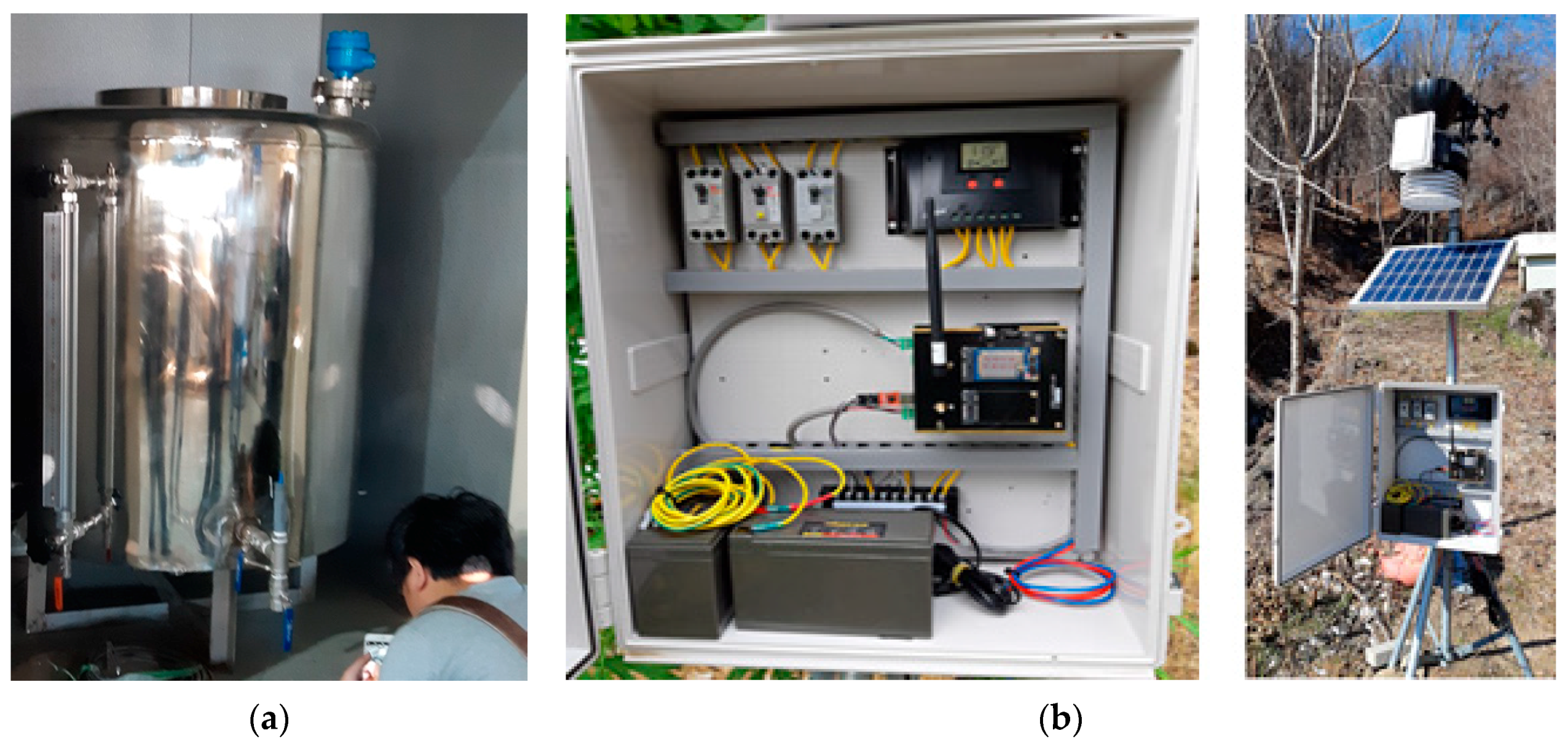
7]. Forest products in deep mountains or alpine zones pose many limits due to their extreme geographical conditions. For data analysis, data should be collected in such alpine zones where there is no smooth supply of electricity. When batteries are used, they are drained quickly due to low temperature, which make it difficult to collect data normally. These problems can be solved with a self-sufficient supply of energy in big data collection devices.
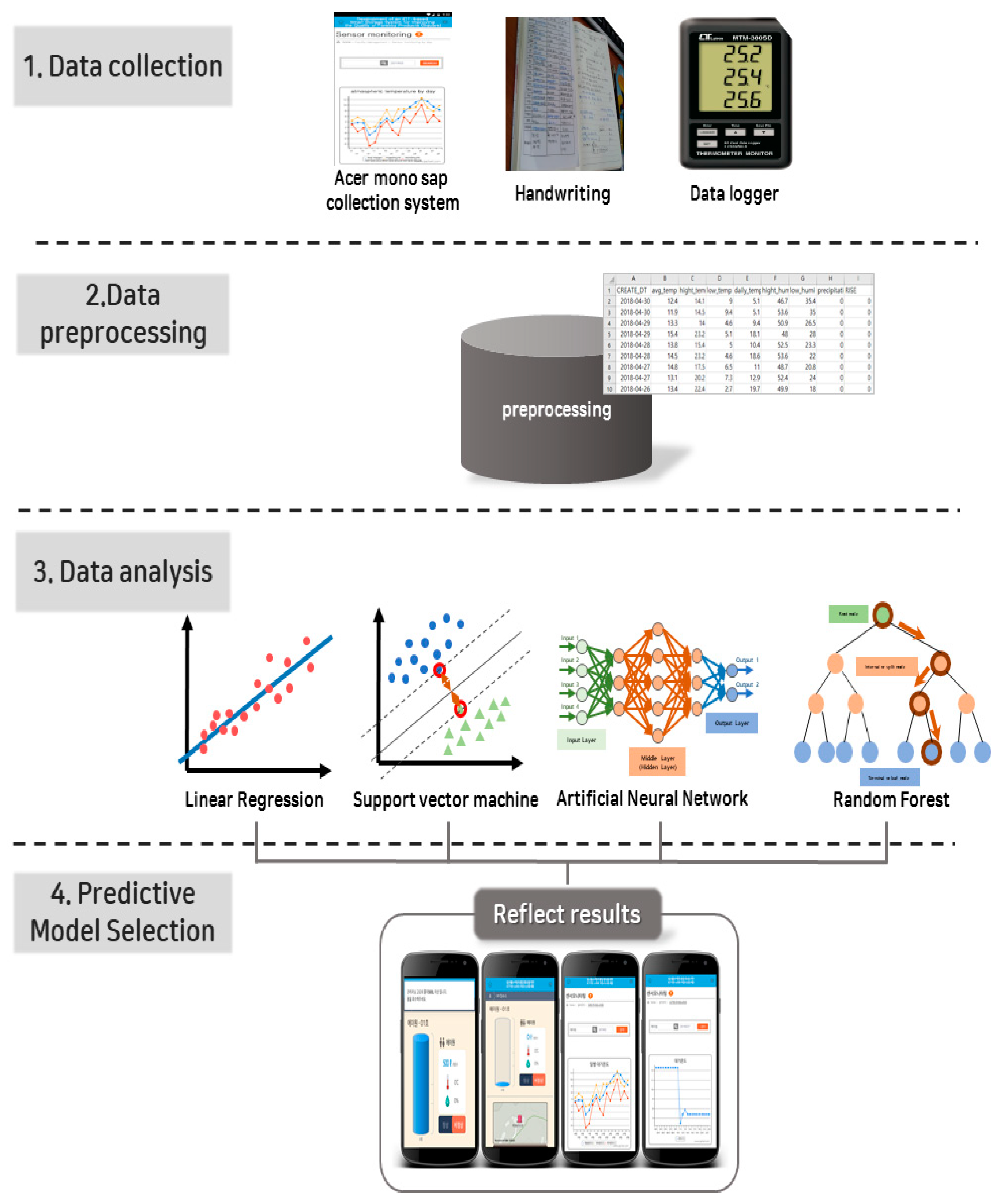
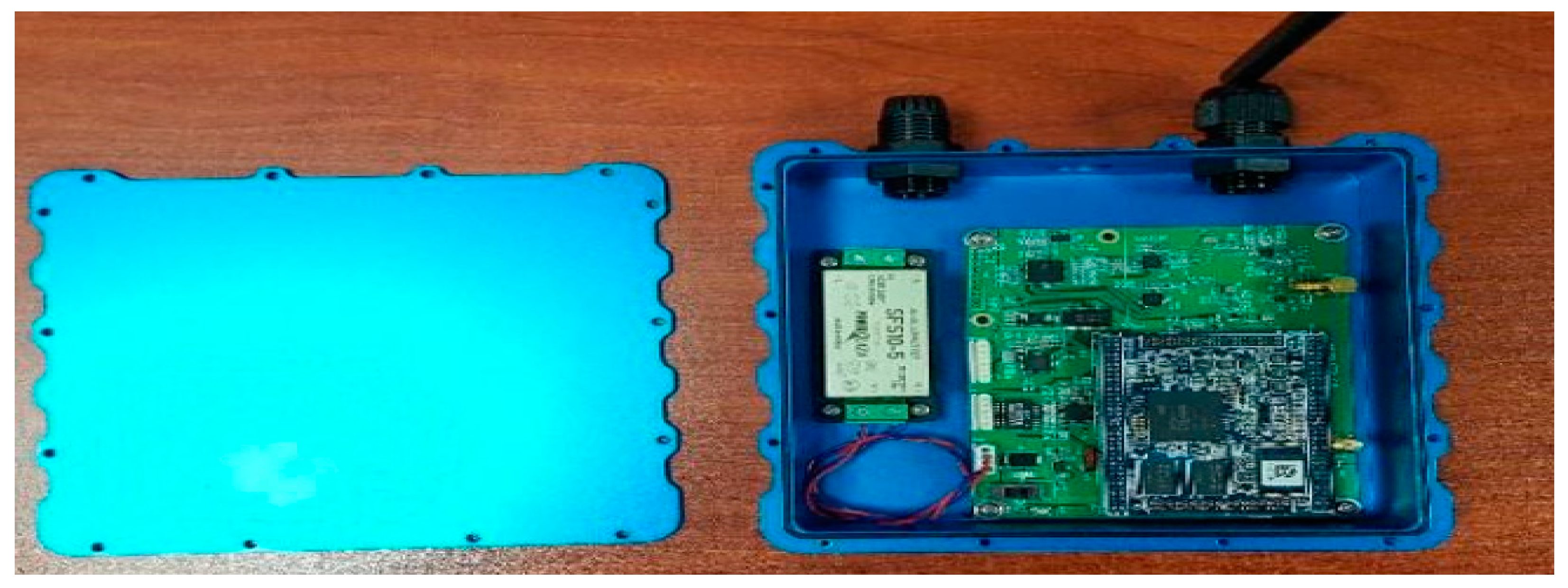
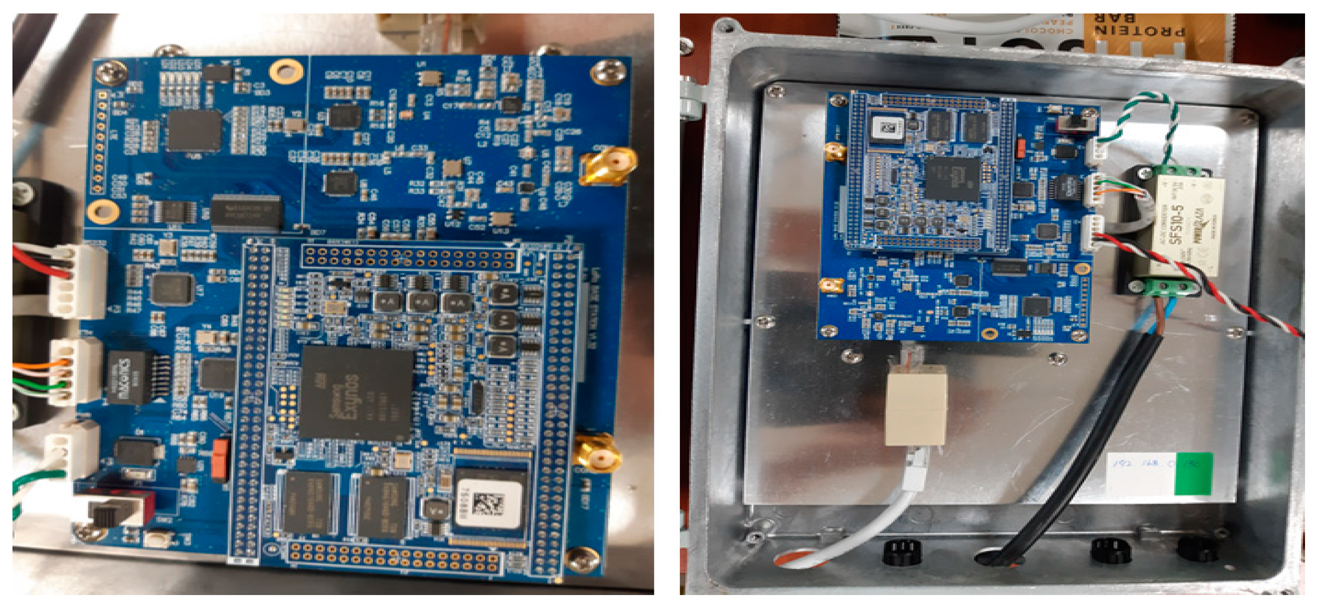
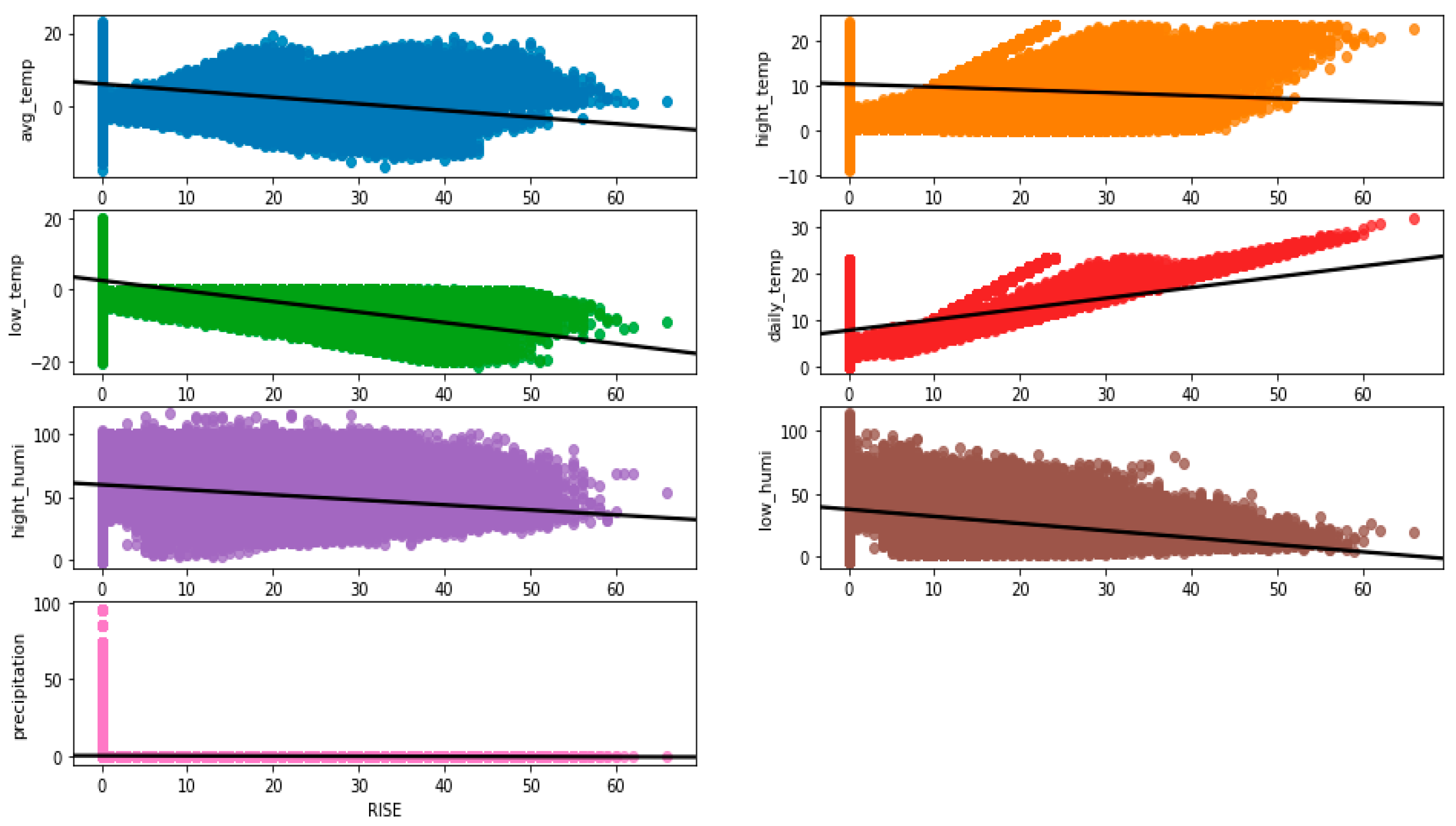
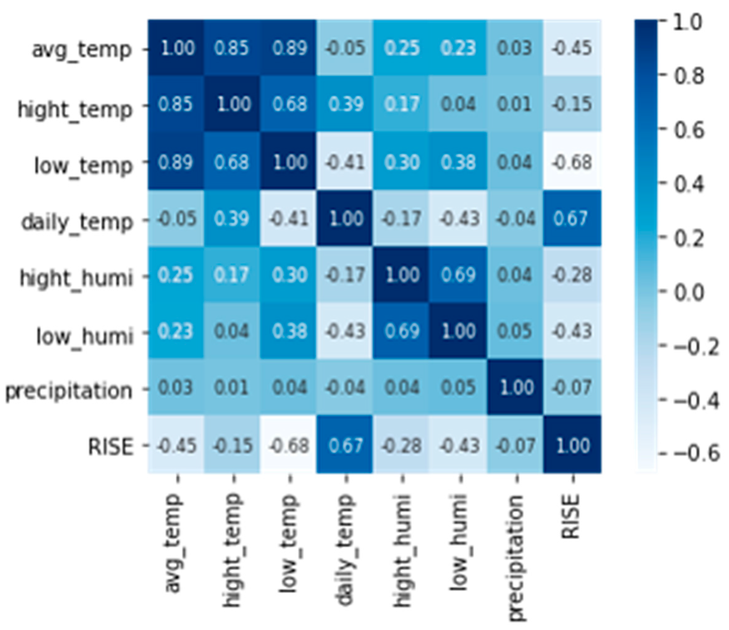
The present study decided to apply the energy harvesting technology to solve these problems. And this study thus set out to develop an ICT-based smart Acer mono sap collection device to promote the efficient utilization of labor force and reduce accident risk by cutting down unnecessary activities, including the manual recording of sap exudation in previous studies, collecting eight factors of environmental data and sap exudation within an hour. Based on farmers’ experiences to suggest close connections between environmental information and Acer mono sap exudation, the study analyzed correlations between them with linear regression, SVM, ANN and random forest and tested a hypothesis with a prediction model for Acer mono sap outputs by the algorithm. Of these prediction models embodied in the study, one was selected for its great availability for a mobile app based on learning hours, prediction hours, and prediction accuracy to provide such data via a mobile app along with environmental information collected with a smart collection device.

2. Proposed Acer Mono Sap Integration Management System

2.1. Overall Block Daigram of Proposed System

Figure 1 shows the overall block diagram of the proposed system. The proposed Acer mono sap storage system consists of hardware and software. The hardware of the system consists of three major parts: a collection device to store sap from Acer mono trees, a big data collection device for data from environmental sensors in and outside the collection device, and a data transmission device to send collects data to the server. The Acer mono sap collection device was made of stainless steel in 1000 L volume. The data collector collected the data of water level, pH, temperature and humidity inside the collection device and the data of outdoor temperature and humidity, ground temperature and humidity, solar radiation, conductivity, wind direction, and velocity. The data transmission device sends data collected from the data collector to the external server via Ethernet and LET communication. In addition, the system software was comprised of an Android-based app to print out data collected from the big data collection device to check it on a mobile terminal in real time and analysis software to analyze correlations between various pieces of environmental information and Acer mono sap yields. The analysis software preprocessed collected data, analyzed correlations with such algorithms as linear regression, SVM, ANN, and random forest, predicted Acer mono sap exudation, and presented the outcomes on a mobile app, which also shows the information about the volume and state of collected sap and external environmental data as well as predicted Acer mono sap exudation in graphs or tables.

2.2. Design of Acer Mono Sap Collection Device

The hardware of the data collection system for Acer mono environment and sap consists of three major parts: the big data collection device to collect data about the meteorological environments of Acer mono sap producing areas scattered in vast zones and the data of sap quality, the ICT-based smart Acer mono sap collection device needed for big data collection, and the communication relay device to collect the sensing data of the sap collection device. Figure 1 (Left) shows the block diagram of the proposed system hardware.
Figure 2 presents the blueprint of the smart collection tank. The old ones simply stored Acer mono sap and did almost nothing for the quality management of collected Acer mono sap in a plastic container.
In the present study, a 1000-L Acer mono sap collection tank was made of stainless steel to prevent corrosion. Measuring devices were added to it to measure temperature, water level, and pH along with communication nodes to collect data. The proposed collection tank was also designed to ensure stable energy supply and eliminate any need for battery replacement by using solar energy panels to control and make use of the energy collected. The energy generated in the photovoltaic modules was supplied to the Acer mono sap collection device and data collection device. The optimal capacity of the energy harvesting device was designed based on the sensors to collect meteorological data and the electric power load and number of sunless days of the sap and data collection devices. Figure 3 shows the power circuit diagram of the energy harvesting-based data collection device. The input power was DC 12 V designed for a stable power supply on the communication board. The power consumption was designed in 3.3 V under 0.5 A for efficient power consumption.
Figure 4 shows a block diagram of the control panel of the smart sap collection device. The control panel was designed for the stable acquisition of sensing data with a programmable logic controller. It can check the current state of Acer mono sap with an electrical box and was designed as a dust- and water-proof panel.

2.3. Design of Monitoring System S/W

The software of the data collection system for Acer mono environment and sap quality used Android-based user monitoring interface. The user interface worked to receive and print out sensor data collected from the data and sap collection devices and save the data in the database after transmitting it to the web server. Figure 5 shows a block diagram of the proposed monitoring software. Figure 6 presents the user’s smartphone application class diagram.
Classes can be defined according to required functions. Methods are processed with each UI button. The login class is for entry into the system and asks the user to provide his or her ID and pin number in the authentication process. The onResume() method is used to generate the instances of connector class and connect them to the server. The login button click event method is used to check IDs and pin numbers. Once users succeed with the login, they will move to the main class, which is connected to the other classes to create instances for each class and enable a transfer to them. The WatertankManager class works to manage the volume of sap and collection in the collection devices and save the data in the database. The WatertankMonitor, WeatherMonitor, and SensorMonitor classes bring the data tables of a farm and show the data about its sap collection devices and weather or sensor data in the button click event method.

2.4. Design of Acer Mono Sap Data Analysis S/W

Figure 7 shows the flow chart of data analysis for the Acer mono sap exudation prediction model proposed in the present study. It consists of four stages. First, data includes the data collected in the study and data from the farmers’ manual books or data loggers. Second, data preprocessing involved unifying the parameters of collected data and removing missing values and outliers having adverse effects on the data analysis. Third, models were tested by selecting an optimal one for each of the algorithms including linear regression, support vector machine, artificial neural network, and random forest. Finally, the most efficient model applicable to a mobile app was chosen to reflect predicted Acer mono sap exudation to a mobile app by comparing the optimal models for each algorithm in predicted accuracy and time.

2.4.1. Big Data Collection

In the present study, data of temperature, humidity, and Acer mono sap for three years was collected from smart sap collection devices attached to 50 Acer mono trees that were 30 years old or older in Sancheong, Gwangyang, Geoje, and Inje. The data was transmitted by an hour and collected on a daily basis. In addition, data was also collected from Acer mono sap farmers’ manual books and data loggers.

2.4.2. Big Data Preprocessing

Outlier data was removed in the preprocessing stage since it could have impacts on the accuracy of Acer mono sap prediction before predicting Acer mono sap exudation with the prediction models. Collected data might include cases influencing Acer mono sap exudation such as the suspension of sap collection due to the sap capacity saturation in the collection device for the day, the cleaning of the rubber tubes to transmit Acer mono sap to the collection devices, and artificial and external problems including damage to the rubber tubes by wild animals. Such data were deemed outliers and thus removed. In addition, missing values whose marks were omitted from the data sets were also removed. The exudation volume was rounded off to a 1 L unit to reduce complexity.

2.4.3. Big Data Type

Data was comprised of components in different forms according to the different collection methods described above. The common elements of different data sets were selected and unified into the components in Table 1 to integrate data sets in different forms into a single form. The integrated data sets had such components as average temperature, highs and lows, daily temperature range, maximum and minimum humidity, and exudation. Up to 66 L of exudation was collected for data. The entire data of 408,864 was randomly divided into learning data of 75% and test data of 25% for the learning and testing of Acer mono sap exudation predictions models. Table 2 shows the data distribution at an interval of approximately 10 L for the rough distribution forms of classified data. The exudation in the range of 60∼66 was an extremely rare case. Since there was an exudation event for each liter, only learning data were organized.
Of the data applied to the study, the avg_temp was in the range of −17.3~23 °C; hight_temp out of a range of −8.9~24.1 °C; the low_temp was in a range of −21.3~20.1 °C; the daily_temp in a range of 0.3~28 °C; hight_humi in a range of 3.2~100%; low_humi in a range of 0.7~100%; precipitation in the range of 0~96 L; and Acer mono sap yielded a range of 0~66 L. A total of 3,270,912 (408,864 × 8) pieces of data were used. Figure 8 shows the amount of data used in the study. The data was mostly concentrated in a certain range. Since graphs displayed numbers too large to be expressed in one place of decimals, some data was not expressed properly. Precipitation was, in particular, classified in details based on numbers. There was an overwhelming number of days when precipitation was 0 (no rain), which made it impossible to express it properly. As for the avg_temp, 3.2 °C recorded the highest numbers at 3754. 7.6 °C recorded the highest numbers at 3124 in hight_temp; −0.3 °C at 5916 in low_temp; 9.3 °C at 4168 in daily_temp; 48% at 1184 in hight_humi; 23% at 1558 in low_humi; 0 L at 403,290 in precipitation; and 0 L at 169,397 in RISE.

3. Experiments and Performance Evaluation

3.1. Implementation of Acer Mono Sap Collection Device

Figure 9a presents the prototype of the smart sap collection tank. Based on the blueprint, a 1000 L Acer mono sap collection tank was made of stainless steel to prevent corrosion. Figure 9b presents the prototype of a new renewable energy-based energy harvesting device, which was installed in the collection areas of Acer mono sap. New renewable energy was used to ensure the smooth supply of electricity to the data collection devices and the generation, storage and supply of electricity. Electrical boxes were added to prevent damage by an external environment and provide dust- and water-proof functions. The new renewable energy system was in a modular structure comprised of storage devices, solar modules, and solar charging controllers for efficiently new renewable energy combinations for the external environment. For its performance assessment, the energy harvesting device was installed in Gwangyang, Jeollanam Province and Sancheong, Gyeongsangnam Province to ensure the smooth supply of power to the sensor nodes.
Figure 10 shows the hardware of communication nodes in the sap collection tank. The nodes collected data of the tank temperature, water level, and pH, and transmits the data via the gateway.
Figure 11 shows the hardware of the multi-channel gateway. The nodes were connected via Ethernet and LET modules for the collection and processing of data transmitted from multiple sensing devices. Outdoor and indoor electrical boxes were made by applying dust- and water-proof features according to the poor external environment so that the multiple-channel gateway could withstand the external environment.

3.2. Implementation of Acer Mono Sap Monitoring System

Figure 12 shows the GUI for users to monitor farmers’ sensing information with a smartphone. The monitoring service consists of sensor data by the hour and date and water level data by the hour and date. Sensor data monitoring by the hour and date offers data of atmospheric temperature and humidity, ground temperature and humidity, EC, solar radiation, and wind direction and velocity. Water level data monitoring by the hour and date helps to check water level changes according to sap collection through the water level sensors in the sap collection devices.

3.3. Evaluation of Acer Mono Sap Output Amount Prediction Model

Based on an assumption that environmental elements around Acer mono trees would have impacts on Acer mono sap exudation based on farmers’ experiences of increasing Acer mono sap exudation according to big daily temperature range due to the osmotic pressure effects and drying and decreasing Acer mono sap exudation according to increased temperature, the present study designed an Acer mono sap exudation prediction model with a total of seven parameters: average temperature, high, low, daily temperature range, maximum humidity, minimum humidity, and precipitation according to four algorithms, i.e., Linear regression [26,27,28,29,30,31,32,33,34,35], SVM [36,37,38,39,40,41,42,43,44,45,46], ANN [47,48,49,50,51,52,53,54,55,56], and Random forest [57,58,59,60,61]. Linear regression predicts and classifies based on linear regression equations derived from the analysis of correlations between dependent and independent variables. This is a technique designed to classify data that cannot be classified linearly, SVM maps data on a hyperplane, defines a decision boundary, and classifies according to the decision boundary. Random forests are an ensemble technique-based classification method of making multiple decision-making trees, gathering classification results from the trees, and presenting a final decision based on the majority result of the most choices. ANN is a machine learning algorithm mimicking the principle and structure of the human neural network. It consists of the input, hidden, and output layer. It solves a problem by learning to find optimal weight and bias with an activation function. The present study found that environmental elements (temperature, humidity, and more) had huge impacts on the yield of Acer mono sap and confirmed first-hand that some of the elements had direct effects on it based on the Acer mono data. Based on the results of previous studies, the study used linear regression to figure out whether there were linear relations between environmental elements and Acer mono sap yield. SVM was also used in a multidimensional mapping method to perform classification based on many different environmental elements. In addition, random forests were used to perform classification according to relationships among the environmental elements and their value. Finally, ANN of high performance in regression and classification was used to develop a model. The models were compared in accuracy with grid searches for hyper-parameters or hidden layers to build and test an optimal model. The optimal models were then compared and analyzed in accuracy, learning time and prediction time by the algorithm to choose one applicable to a mobile app.
Figure 13 shows a confusion matrix to explain the prediction accuracy indicator. Equation (1) expresses precision, and the recall and accuracy based on it. Here, precision represents the actual percentage of True in what is classified as True in the model; recall represents the percentage of what is predicted as True in the model among what is actually True; and accuracy represents the percentage of the right prediction in the entire data.
P r e c i s i o n = T P T P + F P R e c a l l = T P T P + F N A c c u r a c y = T P + T N A l l   P r e d i c t i o n

3.3.1. Linear Regression Model

Based on an assumption that surrounding environmental elements would have impacts on Acer mono sap exudation, the present study selected linear regression as an Acer mono sap exudation prediction model to figure out whether there were linear relations among the elements. The linear regression model underwent OLS to judge and select significant parameters or input variables. In addition, scikit-learn was used to design a multiple linear regression model [26,27,28,29,30,31,32,33,34,35].

OLS

OLS (ordinary least square) is the most basic deterministic linear regression method to obtain the weighted value vector to minimize the residual sum of squares with matrix differentials [31,32,33,34,35]. It can help to check the coefficient and significance probability of each variable by applying regression analysis to preprocessed data. In the data preprocessed in OLS, it was examined whether the independent variables would have effects on the dependent ones (significance probability) to select input variables for the multiple linear regression model. Table 3 shows the outcomes of OLS with all the data after preprocessing. The significance probability of variables was 0.05 or lower in all cases, which means that all seven variables had significant meanings and were thus chosen for the multiple linear regression model as input variables.
Figure 14 shows the correlations between each parameter and amount of sap. There were negative correlations between them except for daily temperature range (daily_temp). The volume of exudation had positive correlations with average temperature (avg_temp) in OLS, which indicates that the independent variables were exchanging influence with one another and that multiple linear regression rather than simple linear regression would be valid for an Acer mono sap exudation prediction model. Equation (2) is for the multiple linear regression model reflecting the OLS outcomes.
Y = 1.2402 + 0.1967 x 1 0.09 x 2 1.2618 x 3 + 1.2528 x 4 0.0227 x 5 0.0229 x 6 0.1352 x 7 + ε
Figure 15 below shows the analysis results based on the interpretations of Pearson’s correlation coefficients between the environmental elements and Acer mono sap yield, which had clear correlations with the avg_temp, low_temp, daily_temp, and low_humi. All the remaining elements had negative correlations with it except for daily_temp. The analysis results indicate that Acer mono sap will record greater yield according to lower average temperature and lows, higher daily temperature range, and lower humidity.

Result of Linear Regression Model

The multiple linear regression model provided its accuracy results of exudation prediction in MAE (mean absolute error), RMSE (root mean squared error), and R 2 . Equation (3) presents methods of expressing prediction accuracy. MAE converts differences between actual and predicted values into absolute ones and obtained their means. RMSE is the root of the mean of difference squares between actual and predicted values. R 2 is the indicator of distribution rate for predicted values against actual ones. The closer it is to 1, the higher prediction accuracy it is. Table 4 shows the prediction results of exudation with the linear regression model. The error mean of absolute values between actual and predicted ones was approximately 5.5. The difference from the observation in an actual environment was 7.12 with a prediction accuracy of 0.649.
M A E = 1 n i = 1 n | Y i Y i ^ | R M S E = 1 n i = 1 n | Y i Y i ^ | R 2 = P r e d i c t e d   V a l u e A c t u a l   V a l u e
Figure 16 shows the current prediction of linear regression. The x axis represents the amount of actual sap, while the y axis represents the predicted amount of sap. The outcomes are presented in dots and the correct answer (red line) of linear function in the y = x form of match between predicted values and correct ones. These outcomes form a prolonged rod shape along the y axis and fail to keep an interval from one another compared with the interval on the x axis, which suggests that the predicted outcomes were printed out in rational numbers rather than integers. Another peculiar aspect to the outcomes is negative values in many predictions. There was also a broad distribution of predicted values lower than the correct ones for the entire data along the red line in the graph. The causes can be found in Equation (3), in which most variables’ weighted values were negative. As a result, predicted values were lower than correct ones in general. These negative predicted values seem to have happened when Acer mono sap was frozen due to low average temperature ( x 1 ) and there was no exudation of Acer mono sap due to absence of osmotic action according to low daily temperature range ( x 2 ).

3.3.2. Support Vector Machine Model

The present study chose SVM (support vector machine) with excellent efficiency in high dimensions as a regression analysis model to be compared with the linear regression model. SVM was embodied with scikit-learn. Since Acer mono sap exudation was predicted in high dimensions with seven parameters, the RBF kernel that was efficient even in high dimensions was used to search for an optimal model [36,37,38,39,40,41,42,43,44,45,46].

Optimization of SVM Model

In SVM, the RBF kernel optimizes a model by regulating gamma and the curvature of the boundary decision according to the influential distance of a data sample. A model was optimized by regulating C (cost) and thus the possibilities of data outliers. Table 5 shows accuracy according to gamma and C values. When C was 0.01 or lower, too many outliers were allowed, which resulted in underfitting. When gamma was lower than 0.001, underfitting happened in which accurate predictions would be impossible due to the increasing overall influence of data samples. When gamma grew to 1 or higher, the sample had smaller influence and resulted in overfitting, in which only learning data would be classified optimally. Overall, high C values led to high accuracy based on the identification of outliers. As data samples had smaller influence, overfitting would happen in which only learning data would be fit with many outliers identified even within the small influence of the samples and lead to lower accuracy.

SVM Optimal Model

The optimal form of SVM model was 0.001 for gamma and 100 for C. Its exudation prediction accuracy was expressed in precision, recall, and accuracy for accurate testing. This method is shown TP represents true positive; FP false positive; FN false negative; and TN true negative. Precision is the percentage of correct ones of predicted values. Recall is the percentage of correct ones of actual values. Accuracy is the overall accuracy of predicted data. Table 6 and Figure 17 shows the prediction accuracy of the optimal SVM model. When the volume of exudation was 0 L, recall was 0.998. The error rate of recall was 0.002 with 101 errors when wrong predicted values were used for the actual value of 0 L. Precision was 0.988. Its error rate was 0.012 with 520 errors when a wrong predicted value of 0 L was used for an actual value that was not 0 L. Precision errors were too many for the support of other exudation data, holding the risk of overfitting toward 0 L. There was a relatively small amount of learning data in the section of 1 L∼9 L with both precision and recall recording mean 0.8 or so. In the section of 10 L∼30 L where there were a lot of data, precision and recall were close to approximately 0.9 in accuracy. As the volume of data decreased in the following sections, precision and recall dropped. Accuracy will grow according to increasing data. The more data there is, the better the outcomes will come out. The current exudation prediction was analyzed in Figure 18, but the outcomes spread wide from the red line according to more data, which suggests that predicted values will have errors of bigger range according to more data. This issue can be found in errors of wide range to predict exudation of 0 L~38 L. When the amount of data is small, on the other hand, the outcomes are closer to the red line. Even though they are not correct ones, predicted and actual values will have similar measurements. The outcomes of the optimal SVM model indicate that learning data will have broad influence due to lower gamma values and that outliers will be identified within the influence due to high C values. This process obtains high results for prediction accuracy, but a big volume of data means bigger influence, which leads to errors in a wider range including the scope of partial outliers with no connections.

3.3.3. Artificial Neural Network Model

ANN (artificial neural network) was chosen as a prediction model in the study since it could make an approximation function from the data used in learning and thus a proper Acer mono sap exudation prediction model. In the present study, ANN was embodied with TensorFlow. In the model, errors were reduced with a cross-entropy function. With the activation function of ReLu (rectified linear unit), the learning rate was set at 0.001 in the learning process to predict the scope of Acer mono sap exudation [47,48,49,50,51,52,53,54,55,56].

Optimization of ANN Model

For model optimization, the middle layer was comprised of multi-layer and deep neural networks with a different number of nodes for each layer as shown in Table 7 and Figure 19. Models A and B are multi-layer neural networks with differences in the number of nodes around a single middle layer. Models C and D are deep neural networks with differences in the number of nodes around five middle layers. These ANN models were examined for accuracy according to the frequency of learning. Table 8 shows prediction accuracy according to the frequency of learning, which includes 1000, 10,000, and 100,000. The models recorded higher accuracy according to increasing learning, but overfitting happened faster according to increasing volume of learning and complexity of models. Models C and D, in particular, recorded the highest accuracy at the learning frequency of 100,000, but they were unstable as their accuracy made a huge drop in the re-testing process three times.

ANN Optimal Model

In ANN, the optimal model was B with the learning frequency of 100,000. Model D had higher accuracy than Model B, but it was unstable as its accuracy went down to 0.44 in the testing process. Being relatively more stable, Model B was chosen as the optimal model. Table 9 shows the prediction accuracy of the optimal ANN model, which recorded high precision and recall values at 1.0 for 0 L of exudation. Table 9 shows the results of rounding off at four decimal places with recall and precision having 15 and two errors for 0 L, respectively. The overall data accuracy was very high at 0.9 or higher. Accuracy was also relatively high even in the section of 47 L~59 L where the amount of data was small. Recall was in the range of 0.6~0.8 for some volumes of exudation, in which phenomenon was estimated to drive from errors based on an incorrect prediction with approximate values as the following volume of exudation had low precision and high recall. Figure 20 shows the current prediction of exudation. At 0 L, there were 15 recall errors. It was the highest at nine for 1 L as an approximate value, being followed by two for 7 L, and one for 17 L, 18 L, 30 L, and 31 L each. There were not many errors other than approximate values, but they were in wide breadth and diversity. Overall predictions were close to the red line, which means overall similarity between actual and predicted values. Some data, however, contained big errors far distant (±7) from the red line with a total of 29 big errors including 4 for 0 L, one for 7 L, five for 14 L, four for 22 L, eight for 23 L, three for 24 L, one for 29 L, and one for 49 L. This phenomenon was more prominent in the sections of more data. The red line also grew thicker in the sections of more data, which can lead to the issue of overfitting like in Models C and D if there is an increase in the amount of learning or complexity of a model.

3.3.4. Random Forest Model

Random forest is an ensemble technique and was selected as an Acer mono sap prediction model in the present study for its possible prediction of greater reliability than a single optimal model. In the present study, random forest was embodied with scikit-learn [23,24,25,57,58,59,60,61].

Optimization of Random Forest Model

To find an optimal random forest model, the present study regulated the number of models (n_estimators) and that of independent variables (max_features) from the data. The other hyper-parameters were kept in the default state during the comparison of models. Table 10 shows the accuracy of random forest models by the hyper-parameter. The bigger the number of independent variables was, the higher accuracy became. The accuracy was the highest when there were a maximum of five independent variables. When the number hit six, however, accuracy dropped a little bit. As the number of models increased, overall accuracy made a small increase as well.

Random Forest Optimal Model

Table 11 and Figure 21 show the prediction accuracy of the optimal model. When the volume of exudation was 0 L, the precision was rounded off to 1.0 with six errors and recall was 0.997 with 122 errors. The big number of recall errors at 0 L had impacts on the overall precision of data, but accuracy was high at 0.9 or higher for most volumes of exudation with stable prediction results. The more data there was, the higher accuracy became. Overall accuracy was low in the section of 50 L~59 L where the pieces of learning data were under 100 per liter. Figure 22 shows the current prediction of random forest for the volume of exudation. At 0 L, there were six precision errors with an approximate value at 1 L. There were 122 recall errors, but it was reduced to a total of 107 after the ones for the approximate value of 1 L were removed. The biggest difference in errors was from the minimum 9 L to maximum 35 L. There were 36 errors for 9 L~19 L, 55 for 20 L~29 L, and 16 for 30 L~35 L. There were a total of 55 errors with a difference of ±2 L or more other than approximate values in addition to 0 L. Errors of a difference of 2 L were the most at 37. There were five with a difference 3 L, six of 4 L, one of 5 L, two of 6 L, one of 7 L, and three of 8 L. There was a big difference between actual and predicted values in about ten cases other than 0 L. In the section of 50 L∼59 L characterized by a small amount of data, most of the values were close to the approximate value (±1) of the correct value contrary to the concern with low prediction accuracy. Only six data points had a difference of ±2 among a total of 115 supports.

3.4. Comparative Evaluation of Optimal Models Between Predicted Models

The optimal models of linear regression, SVM, ANN and random forest algorithms were compared in learning time, prediction time, and accuracy to select one applicable to a mobile app. Learning time represents time required for a model to learn data. It was chosen as a criterion of evaluation for the expandability of a model for additional learning with data collected from Acer mono sap collection devices. Prediction time represents time required for a model to predict Acer mono sap exudation. It was added as a criterion to take into account the time until the outcomes are reflected when users check exudation prediction with a mobile app. Accuracy represents the degree of match between predicted exudation by a model and actual exudation. It was added as another criterion of evaluation to reflect how accurate outcomes can be delivered to users when they check predicted exudation on a mobile app. Table 12 shows the optimal models in learning time, prediction time, and accuracy.
It was the linear regression algorithm that recorded the shortest learning time for a model to learn 306,648 bits of data. The linear regression algorithm calculated weighted values of parameters from learning data to make a linear equation, thus creating a learning model within a short amount of learning time. The SVM algorithm recorded relatively longer learning time as it created a discriminant boundary by selecting support vectors based on the mapping of data in a characteristic space. The ANN algorithm recorded a long learning time as increasing amounts of learning meant higher accuracy for a model. Even though GPU was used to shorten the long learning time, it still recorded the longest time of learning. The random forest algorithm took a short time by doing a relatively simple work of creating random models with bootstrapping to provide outcomes with an ensemble technique. The linear regression and ANN algorithms recorded the shortest prediction time for the test data of 102,216. These two algorithms used weighted values based on learning and underwent a calculation process to provide outcomes, thus recording a short prediction time of less than a second. The SVM algorithm, on the other hand, recorded the longest prediction time as it distinguished data and produced outcomes with a discriminant boundary and did mapping for the test data in the same characteristic space as the learning form. The random forest algorithm recorded a relatively longer prediction time as its final outcomes were based on a majority voting for the results of models(trees) according to the ensemble technique. The random forest algorithm recorded the highest prediction accuracy. In the current predictions of sap exudation by the algorithm (Figure 16, Figure 18, Figure 20 and Figure 22), the algorithm showed the most stable form that was the narrowest to the red line and thus recorded the highest prediction accuracy. The linear regression algorithm recorded very low prediction accuracy of 0.404 even after the compensation of its prediction outcomes for its comparison with other algorithms by converting real numbers into integers and removing negative number predictions with minimum value limited to 0. Both the SVM and ANN algorithms recorded high accuracy, but their exudation predictions were relatively wide along the red line compared with the random forest algorithm, thus leaving room for improvement. The linear regression, SVM, ANN, and random forest algorithms were compared in learning time, prediction time, and accuracy. The linear regression algorithm recorded a short learning and prediction time, but its accuracy was very low, which made it an unfit algorithm for a mobile app to predict sap exudation. The SVM algorithm recorded the highest accuracy, but its learning and prediction was slow. It took a long prediction time due to mapping in a characteristic space even when it used a small amount of test data. The SVM model was thus not fit for a mobile app. The ANN algorithm was slow in learning, but it can be resolved with improved GPU. With its short prediction time and high accuracy, it seems like a fit model to predict sap exudation on a mobile app. The random forest algorithm recorded the highest accuracy and most stable prediction of the models. Its learning time was also short compared with the other models except for linear regression. Its prediction rate was slower than other models, but it recorded as short prediction time as the other models for the data amount of approximately 10,000. The rate issue can be resolved with CPU clock improvement. The random forest model was the fittest of the models to predict sap exudation on a mobile app.

4. Conclusions

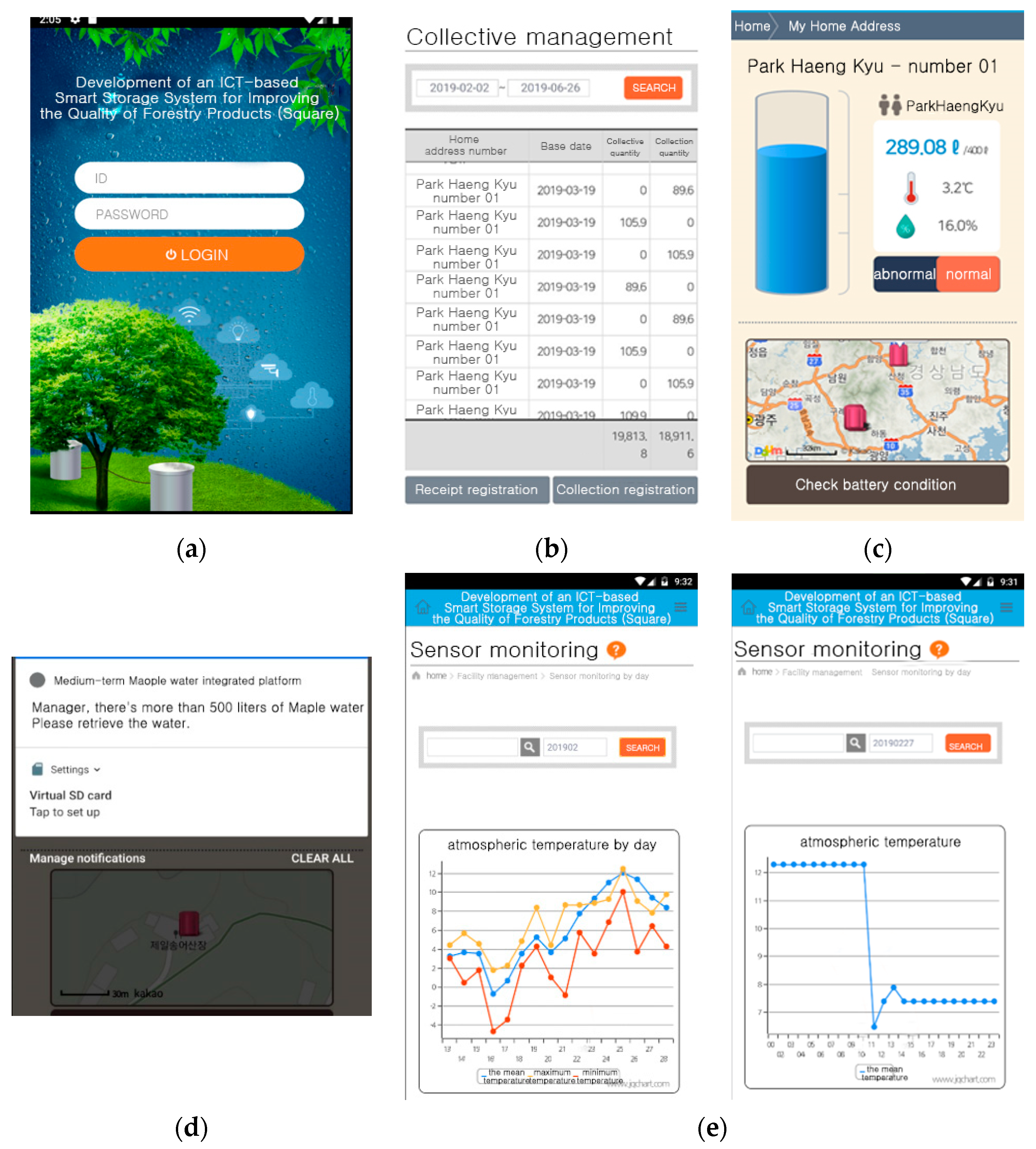
The present study made an Acer mono sap collection device and invented a mobile app for farm managers to check predicted Acer mono sap exudation in real time based on the analysis of data about environmental factors including exudation, outdoor temperature, humidity, conductivity, and wind direction and velocity collected from such a device.
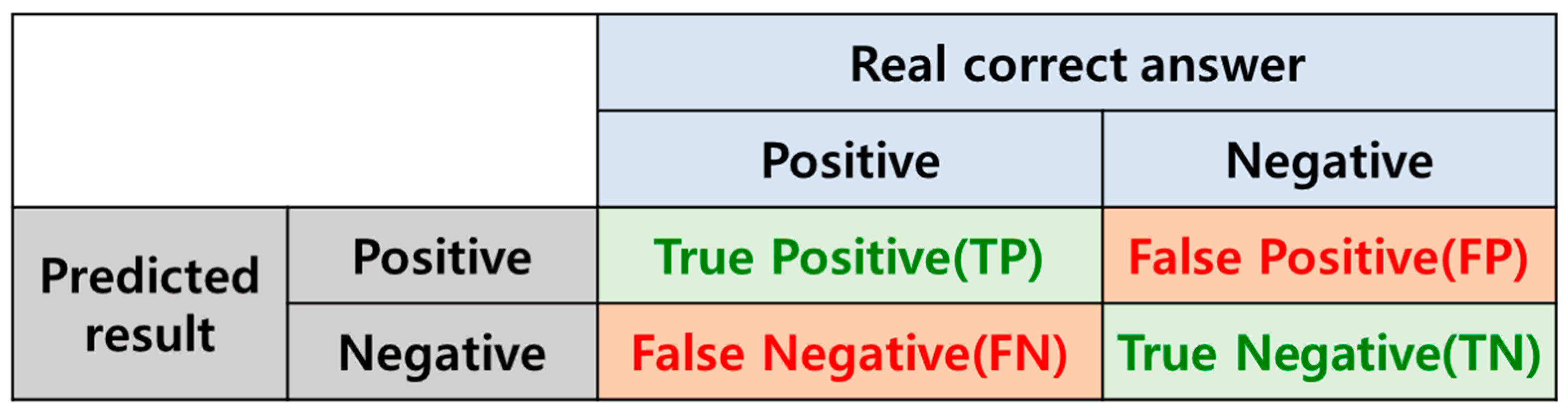
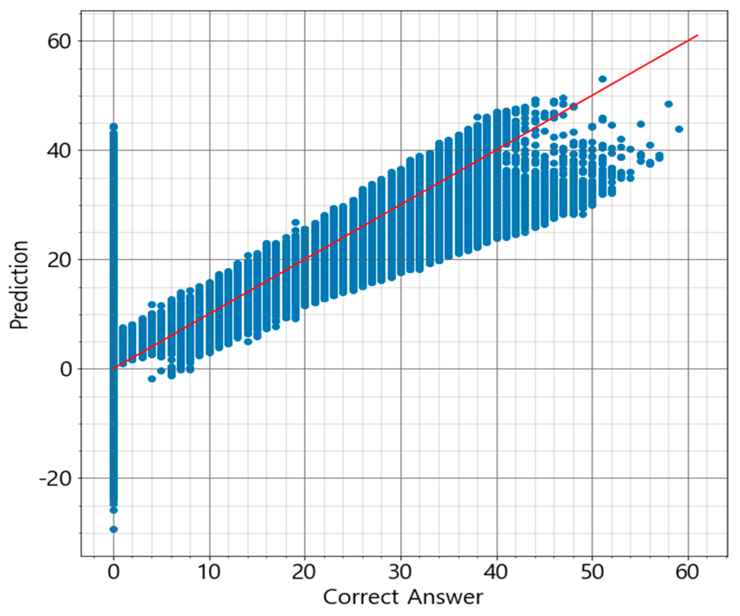
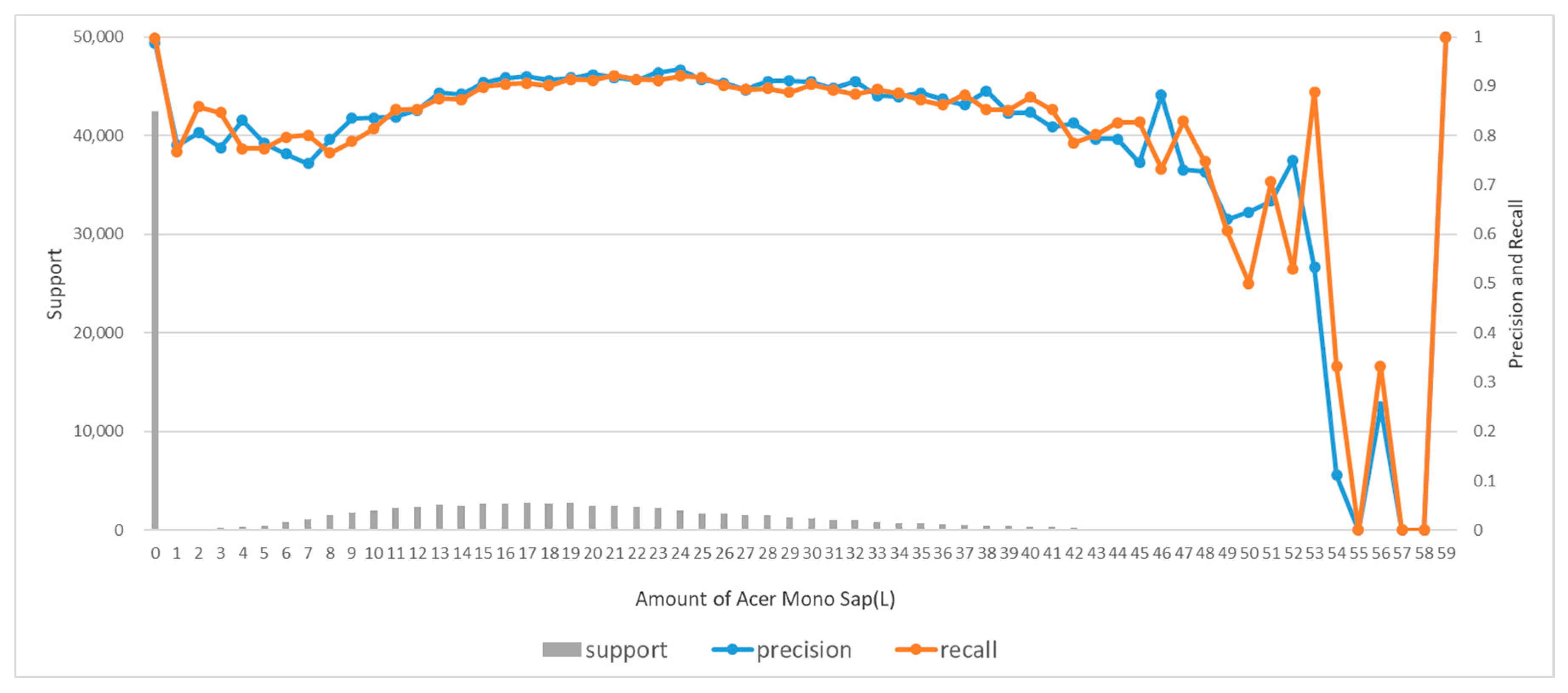
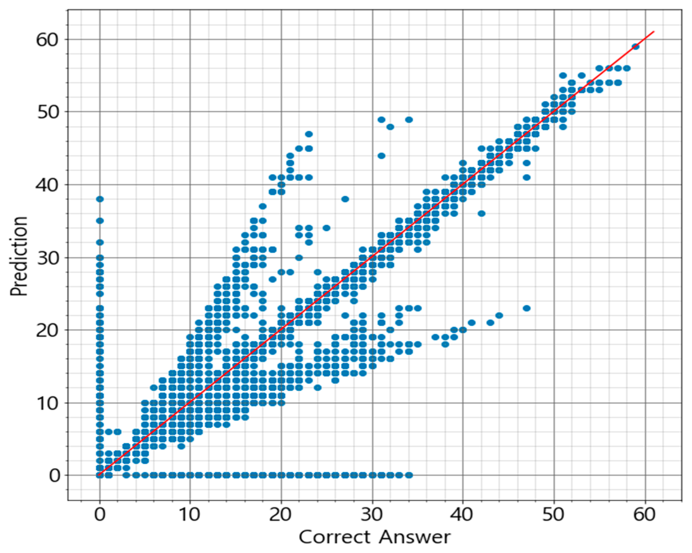
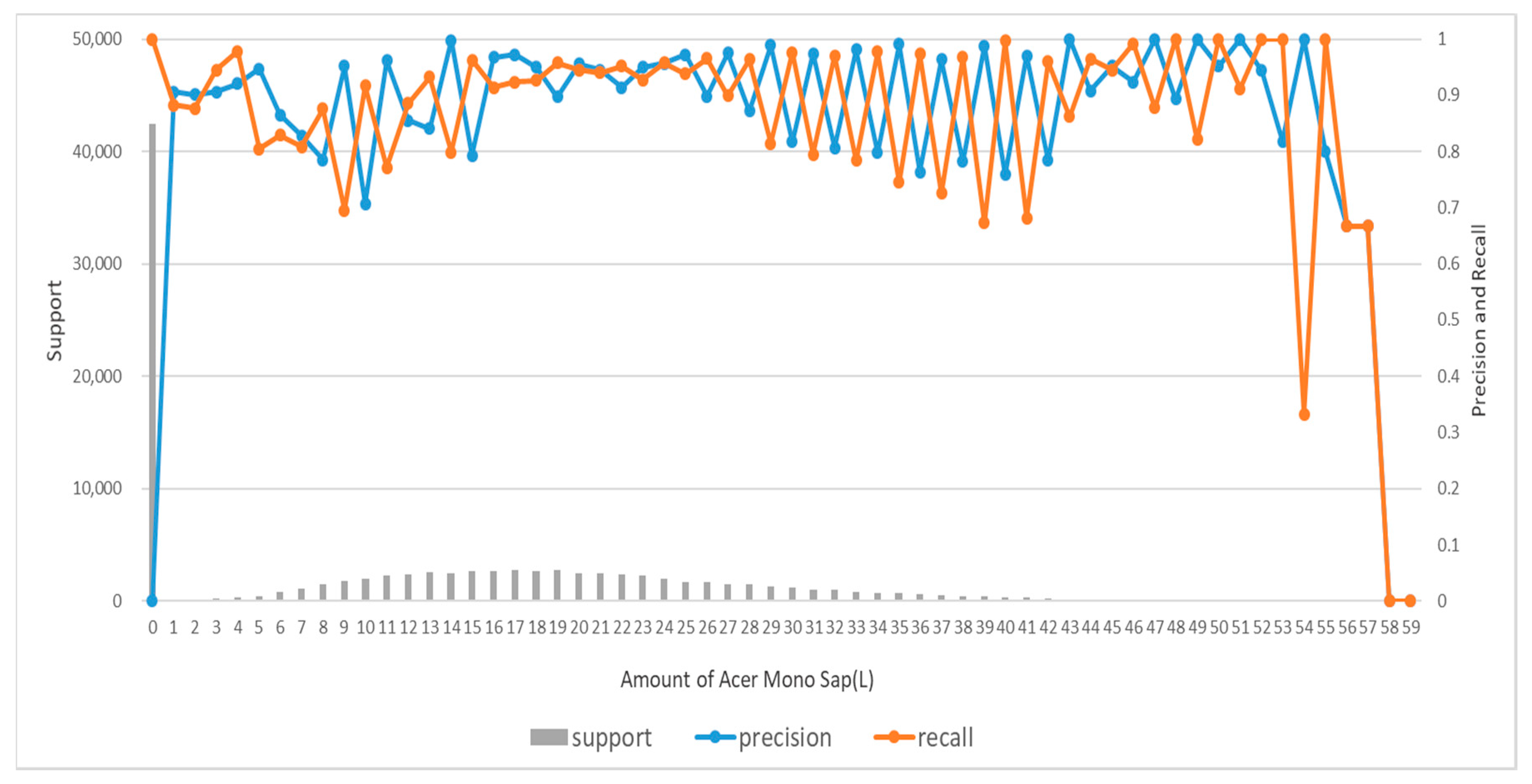
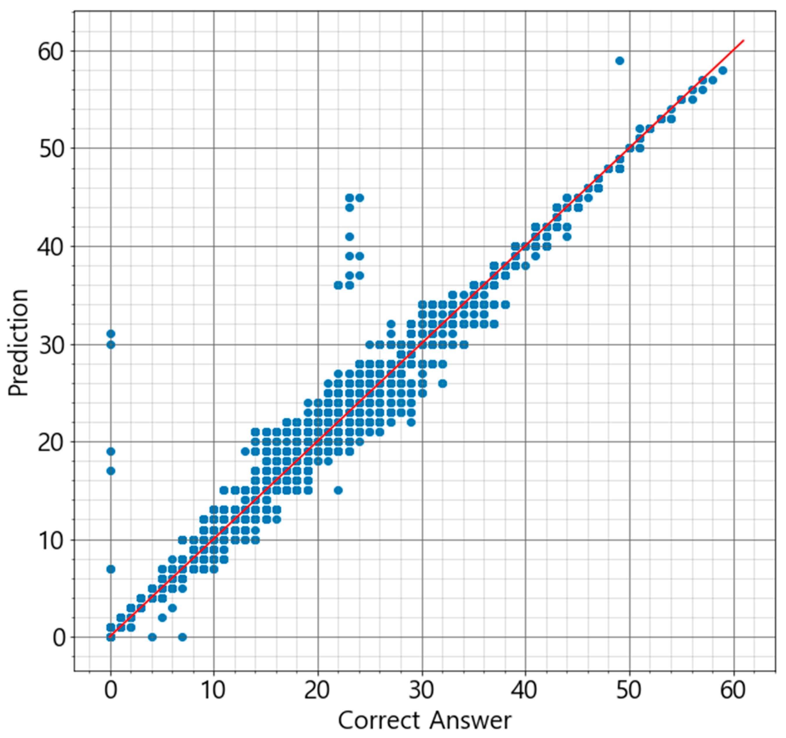
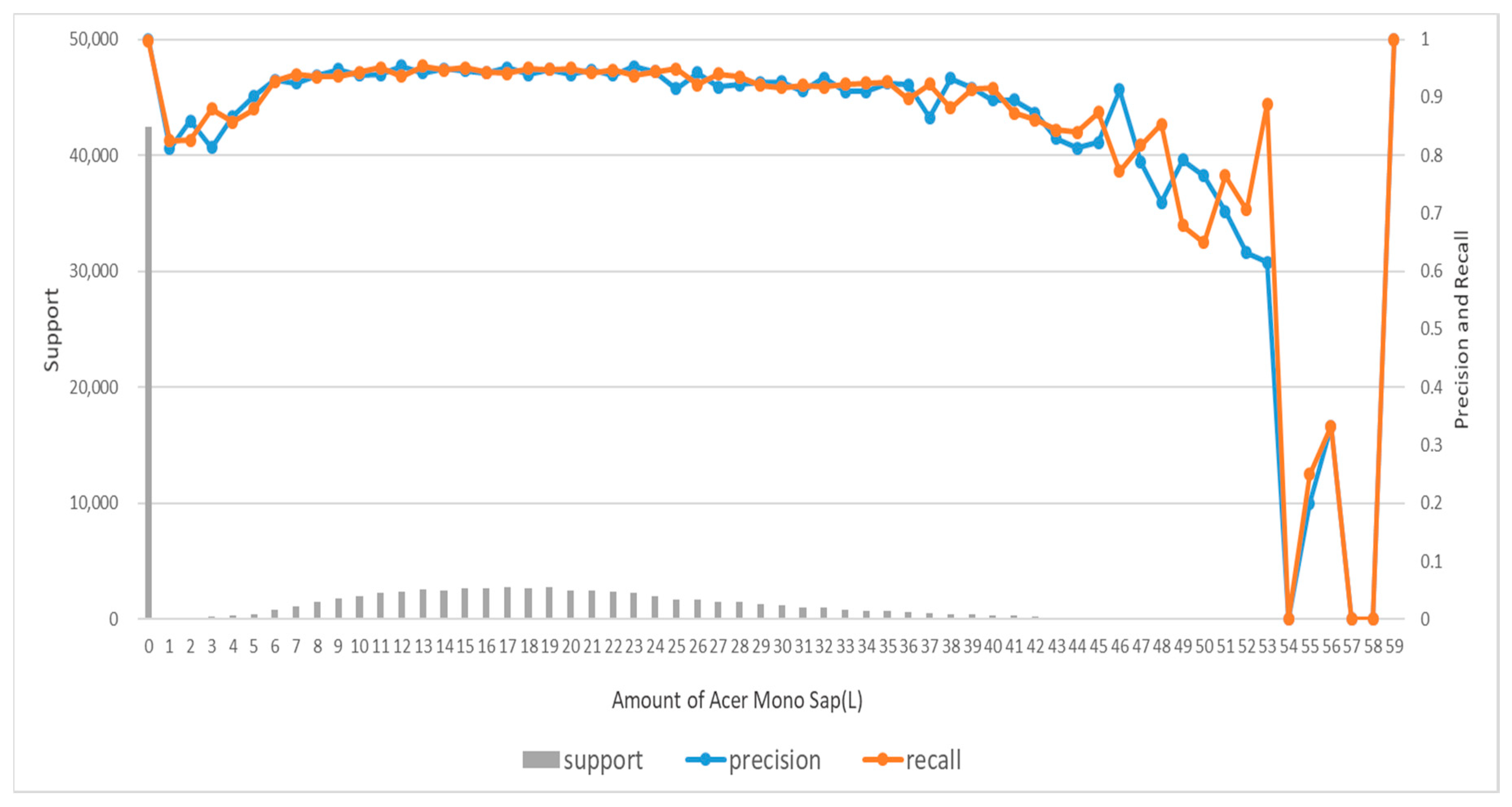
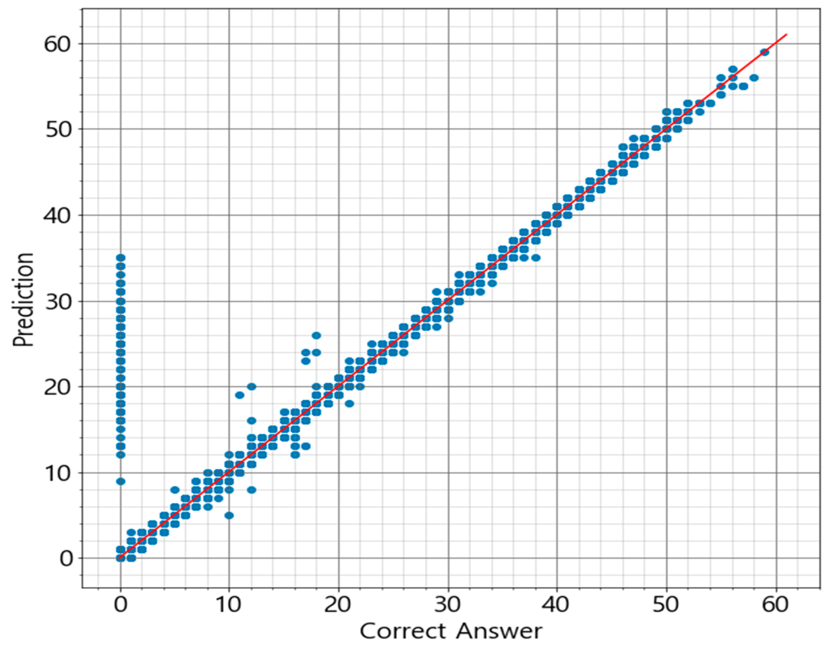
Based on the assumption that Acer mono sap exudation would depend on the environment of Acer mono trees, the study designed prediction models for Acer mono sap exudation with linear regression, SVM, ANN, and random forest algorithms. All the algorithms recorded high prediction accuracy except for linear regression, which confirms the assumption that Acer mono sap exudation would be determined by the surrounding environment. These models were also compared in learning time, prediction time, and accuracy, and the random forest model was chosen to be applicable for a mobile app.
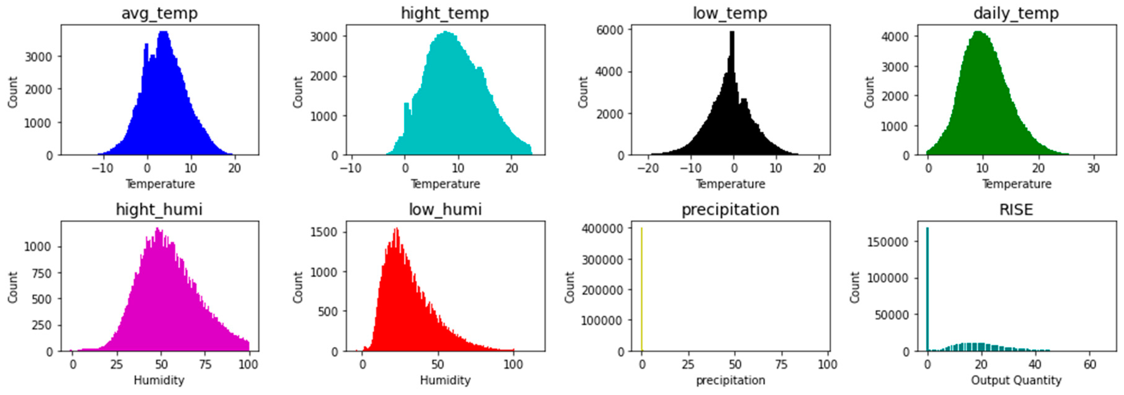
A follow-up study will examine clearer correlations between Acer mono sap exudation and environmental information and design a new algorithm by gathering more data based on the findings of the present study and resolving the data imbalance issue. If the data imbalance issue is not resolved due to climate characteristics, a new approach will be proposed to combine ANN and random forest in an ensemble technique and address the overfitting issue of ANN and the error numbers at 0 L of random forest with the disadvantages of the two algorithms supplemented.

Author Contributions

Conceptualization, S.-H.J., J.-Y.K., J.P., J.-H.H. and C.-B.S.; data curation, S.-H.J., J.-Y.K. and J.-H.H.; formal analysis, J.-Y.K., J.P. and C.-B.S.; funding acquisition, S.-H.J. and C.-B.S.; investigation, S.-H.J. and C.-B.S.; methodology, S.-H.J., J.-Y.K., J.P., J.-H.H. and C.-B.S.; project administration, C.-B.S.; resources, S.-H.J., J.-Y.K., J.P. and J.-H.H.; software, S.-H.J., J.P., J.-H.H. and C.-B.S.; supervision, S.-H.J. and C.-B.S.; validation, J.-Y.K. and C.-B.S.; visualization, S.-H.J., J.-Y.K., J.P., J.-H.H. and C.-B.S.; writing—original draft, S.-H.J., J.-Y.K., J.P., J.-H.H. and C.-B.S.; writing—review & editing, J.-H.H. and C.-B.S. All authors have read and agreed to the published version of the manuscript.

Funding

This work was supported by the National Research Foundation of Korea (NRF) grant funded by the Korea government (MSIT) (NRF-2019R1G1A1002205). And this research was supported by Basic Science Research Program through the National Research Foundation of Korea (NRF) funded by the Ministry of Education (2020R1I1A3054843). And this study was carried out with the support of ‘R&D Program for Forest Science Technology (Project No. 2017090A00-1719-AB01)’ proviede by Korea Forest Service (Korea Forestry Promotion Institute).

Conflicts of Interest

The authors declare no conflict of interest.

Abbreviations

ICTInformation and Communication Technologies
AMSAcer Mono Sap
ANNArtificial Neural Network
SVMSupport Vector Machine
OLSOrdinary Least Square
MAEMean Absolute Error
RMSERoot Mean Squared Error

References

  1. Černý, T.; Kopecký, M.; Petřík, P.; Song, J.-S.; Šrůtek, M.; Valachovič, M.; Altman, J.; Dolezal, J. Classification of Korean forests: Patterns along geographic and environmental gradients. Appl. Veg. Sci. 2014, 18, 5–22. [Google Scholar] [CrossRef]
  2. Liu, C.; Cong, J.; Shen, H.; Lin, C.; Saito, Y.; Ide, Y. Genetic relationships among sympatric varieties of Acer mono in the Chichibu Mountains and Central Hokkaido, Japan. J. For. Res. 2016, 28, 699–704. [Google Scholar] [CrossRef]
  3. Lee, Y.W.; Cho, J.S.; Shin, H.H.; Yoe, H.; Shin, C.S. Construction of Farming-diary Management System Using Ubiquitous Technologies. In Proceedings of the Processing Conference of the Korean Internet Information Society, Cheon-An, Korea, 22 May 2009; pp. 301–305. [Google Scholar]
  4. Ko, D.S.; Park, H.S. The Study for Design of Growth Environment Monitoring System of Vertical Farm. In Proceedings of the Processing Conference of the Korean Information Technical Society, Je-Ju, Korea, 9 December 2011; pp. 372–375. [Google Scholar]
  5. Kwon, D.S.; Lee, B.D.; Jung, J.S. Development of Sap Production Management System of Acer Pictum Var. Mono. In Proceedings of the Processing of Conference the Korean Forest Society, Cheong-Ju, Korea, 27 June 2002; pp. 164–166. [Google Scholar]
  6. Shin, J.-S.; Lee, J.-I. Design and Construction of Farm Management System by U-IT. J. Inst. Webcasting Internet Telecommun. 2012, 12, 285–289. [Google Scholar] [CrossRef] [Green Version]
  7. Wang, Z.-P.; Han, S.-J.; Li, H.-L.; Deng, F.-D.; Zheng, Y.-H.; Liu, H.-F.; Han, X.-G. Methane Production Explained Largely by Water Content in the Heartwood of Living Trees in Upland Forests. J. Geophys. Res. Biogeosci. 2017, 122, 2479–2489. [Google Scholar] [CrossRef]
  8. Lagacé, L.; Leclerc, S.; Charron, C.; Sadiki, M. Biochemical composition of maple sap and relationships among constituents. J. Food Compos. Anal. 2015, 41, 129–136. [Google Scholar] [CrossRef]
  9. Berg, A.K.V.D.; Perkins, T.D.; Isselhardt, M.L.; Wilmot, T.R. Growth Rates of Sugar Maple Trees Tapped for Maple Syrup Production Using High-Yield Sap Collection Practices. For. Sci. 2016, 62, 107–114. [Google Scholar] [CrossRef] [Green Version]
  10. Houle, D.; Paquette, A.; Côté, B.; Logan, T.; Power, H.; Charron, I.; Duchesne, L. Impacts of Climate Change on the Timing of the Production Season of Maple Syrup in Eastern Canada. PLoS ONE 2015, 10, e0144844. [Google Scholar] [CrossRef]
  11. Snyder, S.A.; Kilgore, M.A.; Emery, M.R.; Schmitz, M. Maple Syrup Producers of the Lake States, USA: Attitudes Towards and Adaptation to Social, Ecological, and Climate Conditions. Environ. Manag. 2019, 63, 185–199. [Google Scholar] [CrossRef]
  12. Legault, S.; Houle, D.; Plouffe, A.; Ameztegui, A.; Kuehn, D.; Chase, L.; Blondlot, A.; Perkins, T.D. Perceptions of U.S. and Canadian maple syrup producers toward climate change, its impacts, and potential adaptation measures. PLoS ONE 2019, 14, e0215511. [Google Scholar] [CrossRef] [Green Version]
  13. Tsuruta, K.; Kume, T.; Komatsu, H.; Otsuki, K. Effects of soil water decline on diurnal and seasonal variations in sap flux density for differently aged Japanese cypress (Chamaecyparis obtusa) trees. Ann. For. Res. 2018, 61, 5–18. [Google Scholar] [CrossRef]
  14. Wang, X.; Liu, J.; Sun, Y.; Li, K.; Zhang, Z. Predictive models for radial sap flux variation in coniferous, diffuse-porous and ring-porous temperate trees. J. For. Res. 2017, 28, 51–62. [Google Scholar]
  15. Brinkmann, N.; Eugster, W.; Zweifel, R.; Buchmann, N.; Kahmen, A. Temperate tree species show identical response in tree water deficit but different sensitivities in sap flow to summer soil drying. Tree Physiol. 2016, 36, 1508–1519. [Google Scholar] [CrossRef] [PubMed] [Green Version]
  16. Maguire, T.J.; Templer, P.H.; Battles, J.J.; Fulweiler, R.W. Winter climate change and fine root biogenic silica in sugar maple trees (Acer saccharum): Implications for silica in the Anthropocene. J. Geophys. Res. Biogeosci. 2017, 122, 708–715. [Google Scholar] [CrossRef]
  17. Satir, O.; Berberoglu, S. Crop yield prediction under soil salinity using satellite derived vegetation indices. Field Crop. Res. 2016, 192, 134–143. [Google Scholar] [CrossRef]
  18. Cooper, M.; Technow, F.; Messina, C.; Gho, C.; Totir, L.R. Use of Crop Growth Models with Whole-Genome Prediction: Application to a Maize Multienvironment Trial. Crop. Sci. 2016, 56, 2141–2156. [Google Scholar] [CrossRef] [Green Version]
  19. Huang, X.; Huang, G.; Yu, C.; Ni, S.; Yu, L. A multiple crop model ensemble for improving broad-scale yield prediction using Bayesian model averaging. Field Crop. Res. 2017, 211, 114–124. [Google Scholar] [CrossRef]
  20. Everingham, Y.L.; Sexton, J.; Skocaj, D.; Inman-Bamber, G. Accurate prediction of sugarcane yield using a random forest algorithm. Agron. Sustain. Dev. 2016, 36, 1–9. [Google Scholar] [CrossRef] [Green Version]
  21. Pantazi, X.E.; Moshou, D.; Alexandridis, T.; Whetton, R.L.; Mouazen, A.M. Wheat yield prediction using machine learning and advanced sensing techniques. Comput. Electron. Agric. 2016, 121, 57–65. [Google Scholar] [CrossRef]
  22. Phan, T.N.; Kappas, M. Comparison of Random Forest, k-Nearest Neighbor, and Support Vector Machine Classifiers for Land Cover Classification Using Sentinel-2 Imagery. Sensors 2017, 18, 18. [Google Scholar] [CrossRef] [Green Version]
  23. Couronné, R.; Probst, P.; Boulesteix, A.-L. Random forest versus logistic regression: A large-scale benchmark experiment. BMC Bioinform. 2018, 19, 1–14. [Google Scholar] [CrossRef]
  24. Probst, P.; Wright, M.N.; Boulesteix, A. Hyperparameters and tuning strategies for random forest. Wiley Interdiscip. Rev. Data Min. Knowl. Discov. 2019, 9, 1–15. [Google Scholar] [CrossRef] [Green Version]
  25. Ahmad, I.; Basheri, M.; Iqbal, M.J.; Rahim, A. Performance Comparison of Support Vector Machine, Random Forest, and Extreme Learning Machine for Intrusion Detection. IEEE Access 2018, 6, 33789–33795. [Google Scholar] [CrossRef]
  26. Van Smeden, M.; De Groot, J.A.H.; Moons, K.G.M.; Collins, G.S.; Altman, D.G.; Eijkemans, M.J.C.; Reitsma, J.B. No rationale for 1 variable per 10 events criterion for binary logistic regression analysis. BMC Med. Res. Methodol. 2016, 16, 1–12. [Google Scholar] [CrossRef] [Green Version]
  27. Abadie, A.; Athey, S.; Imbens, G.W.; Wooldridge, J.M. Sampling-Based versus Design-Based Uncertainty in Regression Analysis. Econometrica 2020, 88, 265–296. [Google Scholar] [CrossRef] [Green Version]
  28. Ranganathan, P.; Pramesh, C.S.; Aggarwal, R. Common pitfalls in statistical analysis: Logistic regression. Perspect. Clin. Res. 2017, 8, 148–151. [Google Scholar]
  29. Wilkins, A.S. To Lag or Not to Lag? Re-Evaluating the Use of Lagged Dependent Variables in Regression Analysis. Polit. Sci. Res. Methods 2018, 6, 393–411. [Google Scholar] [CrossRef]
  30. Yao, K.; Liu, B. Uncertain regression analysis: An approach for imprecise observations. Soft Comput. 2018, 22, 5579–5582. [Google Scholar] [CrossRef]
  31. Chen, X.; Wan, A.T.K.; Zhou, Y. Efficient Quantile Regression Analysis With Missing Observations. J. Am. Stat. Assoc. 2015, 110, 723–741. [Google Scholar] [CrossRef]
  32. Judd, C.M.; McClelland, G.H.; Ryan, C.S. Data Analysis: A Model Comparison Approach to Regression, ANOVA, and Beyond; Routledge: Abingdon-on-Thames, UK, 2017. [Google Scholar]
  33. Erik, M.; Sarstedt, M.; Mooi-Reci, I. “Regression Analysis.” Market Research; Springer: Singapore, 2018; pp. 215–263. [Google Scholar]
  34. Donnelly, S.; Verkuilen, J. Empirical logit analysis is not logistic regression. J. Mem. Lang. 2017, 94, 28–42. [Google Scholar] [CrossRef]
  35. Chavas, J.-P. On multivariate quantile regression analysis. J. Ital. Stat. Soc. 2017, 27, 365–384. [Google Scholar] [CrossRef]
  36. Wu, J.; Yang, H. Linear Regression-Based Efficient SVM Learning for Large-Scale Classification. IEEE Trans. Neural Netw. Learn. Syst. 2015, 26, 2357–2369. [Google Scholar] [CrossRef] [PubMed]
  37. Lan, L.; Wang, Z.; Zhe, S.; Cheng, W.; Wang, J.; Zhang, K. Scaling Up Kernel SVM on Limited Resources: A Low-Rank Linearization Approach. IEEE Trans. Neural Netw. Learn. Syst. 2019, 30, 369–378. [Google Scholar] [CrossRef] [Green Version]
  38. Sentelle, C.G.; Anagnostopoulos, G.C.; Georgiopoulos, M. A Simple Method for Solving the SVM Regularization Path for Semidefinite Kernels. IEEE Trans. Neural Netw. Learn. Syst. 2016, 27, 709–722. [Google Scholar] [CrossRef] [PubMed]
  39. Zhang, G.; Piccardi, M. Structural SVM with Partial Ranking for Activity Segmentation and Classification. IEEE Signal Process. Lett. 2015, 22, 2344–2348. [Google Scholar] [CrossRef]
  40. Gu, B.; Sheng, V.S.; Tay, K.Y.; Romano, W.; Li, S. Cross Validation Through Two-Dimensional Solution Surface for Cost-Sensitive SVM. IEEE Trans. Pattern Anal. Mach. Intell. 2016, 39, 1103–1121. [Google Scholar] [CrossRef]
  41. Nguyen, H.-N.; Lee, H.-H. An Effective SVM Method for Matrix Converters With a Superior Output Performance. IEEE Trans. Ind. Electron. 2017, 65, 6948–6958. [Google Scholar] [CrossRef]
  42. Dong, A.; Chung, F.L.K.; Deng, Z.; Wang, S. Semi-Supervised SVM With Extended Hidden Features. IEEE Trans. Cybern. 2015, 46, 2924–2937. [Google Scholar] [CrossRef]
  43. Sun, Z.; Hu, K.; Hu, T.; Liu, J.; Zhu, K. Fast Multi-Label Low-Rank Linearized SVM Classification Algorithm Based on Approximate Extreme Points. IEEE Access 2018, 6, 42319–42326. [Google Scholar] [CrossRef]
  44. Astorino, A.; Fuduli, A. The Proximal Trajectory Algorithm in SVM Cross Validation. IEEE Trans. Neural Netw. Learn. Syst. 2015, 27, 966–977. [Google Scholar] [CrossRef]
  45. Alamdar, F.; Mohammadi, F.S.; Amiri, A. Twin Bounded Weighted Relaxed Support Vector Machines. IEEE Access 2019, 7, 22260–22275. [Google Scholar] [CrossRef]
  46. Eskandarpour, R.; Khodaei, A. Leveraging Accuracy-Uncertainty Tradeoff in SVM to Achieve Highly Accurate Outage Predictions. IEEE Trans. Power Syst. 2018, 33, 1139–1141. [Google Scholar] [CrossRef]
  47. Garro, B.A.; Vázquez, R.A. Designing Artificial Neural Networks Using Particle Swarm Optimization Algorithms. Comput. Intell. Neurosci. 2015, 2015, 1–20. [Google Scholar] [CrossRef]
  48. Bas, E. The Training Of Multiplicative Neuron Model Based Artificial Neural Networks With Differential Evolution Algorithm For Forecasting. J. Artif. Intell. Soft Comput. Res. 2016, 6, 5–11. [Google Scholar] [CrossRef] [Green Version]
  49. Manngård, M.; Kronqvist, J.; Böling, J.M. Structural learning in artificial neural networks using sparse optimization. Neurocomputing 2018, 272, 660–667. [Google Scholar] [CrossRef]
  50. Yang, Z.; Lin, D.K.; Zhang, A. Interval-valued data prediction via regularized artificial neural network. Neurocomputing 2019, 331, 336–345. [Google Scholar] [CrossRef] [Green Version]
  51. Xu, F.; Pun, C.-M.; Li, H.; Zhang, Y.; Song, Y.; Gao, H. Training Feed-Forward Artificial Neural Networks with a modified artificial bee colony algorithm. Neurocomputing 2020, 416, 69–84. [Google Scholar] [CrossRef]
  52. Gazder, U.; Shakshuki, E.M.; Adnan, M.; Yasar, A.-U.-H. Artificial Neural Network Model to relate Organization Characteristics and Construction Project Delivery Methods. Procedia Comput. Sci. 2018, 134, 59–66. [Google Scholar] [CrossRef]
  53. Lakshmanan, I.; Ramasamy, S. An Artificial Neural-Network Approach to Software Reliability Growth Modeling. Procedia Comput. Sci. 2015, 57, 695–702. [Google Scholar] [CrossRef] [Green Version]
  54. Gonzalez, J.; Yu, W. Non-linear system modeling using LSTM neural networks. IFAC-PapersOnLine 2018, 51, 485–489. [Google Scholar] [CrossRef]
  55. Melin, P.; Sánchez, D. Multi-objective optimization for modular granular neural networks applied to pattern recognition. Inf. Sci. 2018, 460, 594–610. [Google Scholar] [CrossRef]
  56. Rhazali, K.; Lussier, B.; Schön, W.; Geronimi, S. Fault Tolerant Deep Neural Networks for Detection of Unrecognizable Situations. IFAC-PapersOnLine 2018, 51, 31–37. [Google Scholar] [CrossRef]
  57. Belgiu, M.; Drăguţ, L. Random forest in remote sensing: A review of applications and future directions. ISPRS J. Photogramm. Remote Sens. 2016, 114, 24–31. [Google Scholar] [CrossRef]
  58. Paul, A.; Mukherjee, D.P.; Das, P.; Gangopadhyay, A.; Chintha, A.R.; Kundu, S. Improved Random Forest for Classification. IEEE Trans. Image Process. 2018, 27, 4012–4024. [Google Scholar] [CrossRef]
  59. Lakshmanaprabu, S.K.; Shankar, K.; Ilayaraja, M.; Nasir, A.W.; Vijayakumar, V.; Chilamkurti, N. Random forest for big data classification in the internet of things using optimal features. Int. J. Mach. Learn. Cybern. 2019, 10, 2609–2618. [Google Scholar] [CrossRef]
  60. Zhou, Y.; Qiu, G. Random forest for label ranking. Expert Syst. Appl. 2018, 112, 99–109. [Google Scholar] [CrossRef] [Green Version]
  61. Nadi, A.; Moradi, H. Increasing the views and reducing the depth in random forest. Expert Syst. Appl. 2019, 138, 112801. [Google Scholar] [CrossRef]
Figure 1. Overall block diagram of proposed system.
Electronics 09 01979 g001
Figure 2. Blueprint of smart collection tank.
Electronics 09 01979 g002
Figure 3. Configuration of energy harvesting.
Electronics 09 01979 g003
Figure 4. Control board of smart collection tank.
Electronics 09 01979 g004
Figure 5. Block diagram of Acer mono sap monitoring.
Electronics 09 01979 g005
Figure 6. User smartphone application class diagram.
Electronics 09 01979 g006
Figure 7. Flow chart of Acer mono sap data analysis.
Electronics 09 01979 g007
Figure 8. The statistical information of the used data set.
Electronics 09 01979 g008
Figure 9. Prototype of Acer mono sap collection H/W. (a) smart sap collection tank; (b) energy harvesting device.
Electronics 09 01979 g009
Figure 10. The communication node of sap collection tank.
Electronics 09 01979 g010
Figure 11. The board of multi-channel gateway.
Electronics 09 01979 g011
Figure 12. Monitoring UI of Acer mono sap. (a) main; (b) sap output; (c) farm information; (d) collection tank push; (e) sensor monitoring.
Electronics 09 01979 g012
Figure 13. Confusion matrix.
Electronics 09 01979 g013
Figure 14. Correlations between variable and amount of sap.
Electronics 09 01979 g014
Figure 15. The analysis results based on the interpretations of Pearson’s correlation coefficients between the environmental elements and Acer mono sap yield.
Electronics 09 01979 g015
Figure 16. Prediction of sap amount based on Liner Regression.
Electronics 09 01979 g016
Figure 17. Prediction accuracy of SVM optimal model.
Electronics 09 01979 g017
Figure 18. Prediction of sap amount based on SVM.
Electronics 09 01979 g018
Figure 19. Prediction accuracy of ANN optimal model.
Electronics 09 01979 g019
Figure 20. Prediction of sap amount based on ANN.
Electronics 09 01979 g020
Figure 21. Prediction accuracy of Random Forest optimal model.
Electronics 09 01979 g021
Figure 22. Prediction of sap amount based on Random Forest.
Electronics 09 01979 g022
Table 1. Element of data set.
Big Data NameVariable NameDescription
Average Temperatureavg_tempDaily Average Temperature
Maximum Temperaturehight_tempDaily Maximum Temperature
Minimum Temperaturelow_tempDaily Minimum Temperature
Daily Temperature Rangedaily_tempDaily Temperature Range (Max. to Min.)
Maximum Humidityhight_humiDaily Maximum Humidity
Minimum Humiditylow_humiDaily Minimum Humidity
Amount of RainfallprecipitationDaily Amount of Rainfall
Acer Mono Sap Output AmountRISEDaily Acer Mono Sap Output Amount
Table 2. Classification of learning data and test data.
Amount of SapAmount of DataLearning DataTest Data
0169,397126,94642,451
1~925,40819,0426366
10~19101,27476,14825,126
20~2976,83757,68319,154
30~3929,05421,6657389
40~49645148361615
50~59438323115
60~66550
Total Data408,864306,648102,216
Table 3. Result of OLS.
VariableCoef.p > |t|
intercept−1.29330.000
avg_temp0.19670.000
hight_temp−0.00900.017
low_temp−1.26180.000
daily_temp1.25280.000
hight_humi−0.22270.000
low_humi−0.02290.000
precipitation−0.13520.000
Table 4. Prediction result of sap amount based on Liner Regression.
MAERMSE Variance   Score   ( R 2 )
5.4877.1200.649
Table 5. Accuracy by SVM hyperparameter.
HyperparameterC = 0.001C = 0.01C = 0.1C = 1C = 10C = 100
Gamma = 0.0010.4150.4170.5300.7660.8980.922
Gamma = 0.010.4150.4410.5780.8470.9080.927
Gamma = 0.10.4160.4170.5300.7660.8210.820
Gamma = 10.4150.4150.4150.4150.4150.415
Gamma = 100.4150.4150.4150.4160.4170.417
Gamma = 1000.4150.4150.4150.4160.4160.416
Table 6. Prediction accuracy of SVM optimal model.
Sap (L)PrecisionRecallSupport
00.9880.99842,451
10.7800.767120
20.8060.858155
30.7750.847183
40.8310.773273
50.7840.773441
60.7630.797803
70.7430.8011098
80.7920.7651486
90.8350.7881807
100.8360.8131970
110.8380.8522241
120.8510.8532332
130.8870.8752552
140.8840.8732512
150.9070.8982658
160.9170.9042677
170.9200.9062775
180.9120.9012672
190.9170.9142737
200.9240.9122489
210.9180.9222436
220.9130.9142320
230.9280.9122237
240.9330.9212008
250.9130.9181733
260.9060.9011718
270.8920.8931515
280.9100.8951451
290.9110.8881247
300.9090.9031198
310.8950.8921030
320.9100.884963
330.8810.893788
340.8790.886745
350.8870.872701
360.8740.862594
370.8620.883522
380.8900.852466
390.8460.851382
400.8470.878335
410.8170.852283
420.8250.785223
430.7930.802167
440.7930.826144
450.7450.827127
460.8820.732123
470.7310.82982
480.7270.74775
490.6300.60756
500.6450.50040
510.6670.70634
520.7500.52917
530.5330.8899
540.1110.3333
550.0000.0004
560.2500.3333
570.0000.0003
580.0000.0001
591.0001.0001
Macro Avg.0.7780.783102,216
Weighted Avg.0.9280.928102,216
Accuracy0.928
Table 7. Configuration of ANN model.
Hidden LayerModel
ABCD
1520520
2--626
3--728
4--618
5--515
Table 8. Prediction accuracy of model based on ANN learning volume.
Prediction VolumeLearning Model
ABCD
10000.4020.4020.3710.414
10,0000.4150.6230.6530.415
100,000 (1)0.8590.8930.9170.952
100,000 (2)0.8800.9400.4150.440
100,000 (3)0.8970.9120.4140.862
Table 9. Prediction accuracy of ANN optimal model.
Sap (L)PrecisionRecallSupport
01.0001.00042,451
10.9060.883120
20.9010.877155
30.9060.945183
40.9210.978273
50.9470.805441
60.8650.829803
70.8280.8091098
80.7850.8761486
90.9520.6951807
100.7070.9171970
110.9620.7712241
120.8550.8862332
130.8410.9322552
140.9980.7992512
150.7930.9632658
160.9680.9142677
170.9720.9242775
180.9500.9272672
190.8970.9582737
200.9560.9452489
210.9450.9402436
220.9140.9522320
230.9500.9282237
240.9570.9582008
250.9720.9381733
260.8980.9661718
270.9750.8991515
280.8720.9641451
290.9890.8141247
300.8170.9761198
310.9740.7951030
320.8070.970963
330.9810.784788
340.7980.977745
350.9910.745701
360.7640.973594
370.9640.726522
380.7820.968466
390.9880.673382
400.7590.997335
410.9700.682283
420.7840.960223
431.0000.862167
440.9080.965144
450.9520.945127
460.9240.992123
471.0000.87882
480.8931.00075
491.0000.82156
500.9521.00040
511.0000.91234
520.9441.00017
530.8181.0009
541.0000.3333
550.8001.0004
560.6670.6673
570.6670.6673
580.0000.0001
590.0000.0001
Macro Avg.0.8710.854102,216
Weighted Avg.0.9460.941102,216
Accuracy0.94
Table 10. Accuracy by Random Forest Hyperparameter.
Hyperparametern_estimators = 100n_estimators = 200n_estimators = 300
max_features = 10.8850.8920.893
max_features = 20.9270.9280.929
max_features = 30.9490.9500.950
max_features = 40.9580.9570.958
max_features = 50.9590.9600.960
max_features = 60.9560.9580.958
max_features = 70.9530.9530.954
Table 11. Prediction accuracy of Random Forest optimal model.
Sap (L)PrecisionRecallSupport
01.0000.99742,451
10.8110.825120
20.8590.826155
30.8130.880183
40.8670.857273
50.9020.880441
60.9290.928803
70.9250.9391098
80.9370.9351486
90.9480.9361807
100.9380.9431970
110.9390.9512241
120.9540.9362332
130.9420.9542552
140.9490.9472512
150.9460.9512658
160.9420.9432677
170.9510.9412775
180.9390.9502672
190.9480.9482737
200.9390.9502489
210.9470.9422436
220.9380.9472320
230.9530.9372237
240.9440.9442008
250.9150.9491733
260.9420.9221718
270.9180.9401515
280.9220.9351451
290.9260.9211247
300.9270.9171198
310.9110.9211030
320.9330.918963
330.9100.923788
340.9100.925745
350.9250.927701
360.9220.897594
370.8650.923522
380.9320.882466
390.9160.914382
400.8950.916335
410.8950.873283
420.8730.861223
430.8290.844167
440.8120.840144
450.8220.874127
460.9130.772123
470.7880.81782
480.7190.85375
490.7920.67956
500.7650.65040
510.7030.76534
520.6320.70617
530.6150.8899
540.0000.0003
550.2000.2504
560.3330.3333
570.0000.0003
580.0000.0001
591.0001.0001
Macro Avg.0.8250.832102,216
Weighted Avg.0.9610.961102,216
Accuracy0.96
Table 12. Comparison of model performance by prediction method.
Prediction MethodLinear RegressionSVMANNRandom Forest
Learning Time00:00:0100:29:2101:32:4400:01:55
Prediction Time00:00:0000:14:5800:00:0000:00:10
Accuracy0.4040.9200.9480.96
Publisher’s Note: MDPI stays neutral with regard to jurisdictional claims in published maps and institutional affiliations.

