Article

A Heterogeneous Inductive Power Transfer System for Electric Vehicles with Spontaneous Constant Current and Constant Voltage Output Features

1
College of Electrical Engineering, Zhejiang University, Hangzhou 310027, China
2
School of Automation, Hangzhou Dianzi University, Hangzhou 310000, China
*
Author to whom correspondence should be addressed.
Electronics 2020, 9(11), 1978; https://doi.org/10.3390/electronics9111978
Submission received: 29 October 2020 / Revised: 16 November 2020 / Accepted: 19 November 2020 / Published: 23 November 2020
(This article belongs to the Section Power Electronics)

Abstract

:
An inductively coupled wireless power transfer system is proposed in this paper, which is designed to comply with the battery’s load characteristics. A loosely coupled transformer with high coupling coefficient is proposed. A heterogeneous compensation topology is proposed which is able to switch between constant current and constant voltage output mode according to the load resistance. The output characteristic curve agrees with the charging curve of the battery in a whole cycle. The proposed topology has a misalignment range of 300 mm where the coupling coefficient is 0.2. A 3 kW experimental platform is established to verify the theoretical analysis, and the experimental results show that the proposed loosely coupled transformer has high coupling coefficient and high power transmission efficiency (95.2% in aligned position) within a large misalignment range, which agrees with the charging scenario of the electric vehicle.

1. Introduction

Inductive power transfer (IPT) realizes power transmission in a contact-less way [1,2], and this technique has been proven to be an ideal technical solution in various applications, like consumer electronics, biomedical implant devices, an underwater power supply, ball-joint structures [3], high-voltage insulation [4], and especially electric vehicles (EVs) [5]. Compared with the conventional “plug-in” charging method, wireless charging features electrical isolation between the primary and secondary side, and can thus be used in bad weather conditions. Moreover, wireless charging eliminates mechanical contact, which lowers the danger of operators getting an electric shock.
The lithium battery is widely applied in electric vehicles as the energy storage unit. The typical charging process of a lithium battery starts with constant current phase and, as the battery voltage increases, the charging scenario switches to constant voltage mode [6,7]. The typical charging curve for a lithium battery is shown in Figure 1. To extend the battery’s service life, the charging system is intended to maintain the precise voltage and current to satisfy the battery’s requirements.
The typical diagram of an inductive charging system is shown in Figure 2. Inductive power transfer system contains the high-frequency inverter, magnetic coupling transformers, resonant compensation topology and rectifier. Usually the IPT system’s compensation parameters and operating frequency are designed with specific output requirements, and the system’s output is influenced by the load conditions.
Typical transformer structures of the WPT (wireless power transfer) system include a circular structure, DD structure (which is composed of two circular coils in reverse series) and solenoid structure [8,9,10,11,12] (shown in Figure 3). The circular winding is distributed circularly in a plane, ferrite strips are placed on the back to guide the magnetic flux and shield magnetic leakage, but the coupling coefficient is low and this structure is sensitive to misalignment. In a DD structure, the magnetic flux flows in from one coil and flows out from another. The general coupling coefficient is improved, but there exists a zero-coupling position at which energy cannot be transferred from the primary side to secondary side. The solenoid structure features a high coupling coefficient, and the zero-coupling position is eliminated; an aluminium plate is always placed on the back to shield the magnetic field leakage. The bipolar transformer has two receiver coils on the secondary side, and when the two coils are overlapped and placed at a certain position, the coupling coefficient between two receiver coils is zero. (Assuming one receiver coil is excited with current, the part of the magnetic flux flowing into the other coil is canceled by the part which flows out of it, and the magnetic field generated by one coil will not induce electromotive force in another.)
The IPT system output is determined by compensation parameters, operating frequency and load condition. Usually the IPT system’s compensation parameters and operating frequency are fixed, and the system’s output varies with load conditions [13,14]. As the equivalent resistance of the battery increases during the constant current mode (the equivalent resistance of the battery is defined as Vbat/Ibat), it is of significance for the system to maintain the required charging current and voltage against a wide load variation range. Researches on CC-CV (constant current-constant voltage) hybrid compensation topology have been reported in previous literature. Southeast University and Hong Kong Polytechnic University [15] proposed a hybrid compensation topology to realize the switch between CC-CV mode. Appropriate alternating current (AC) switches are needed in order to change the topologies between two modes [16]. Y. Li et al. systematically investigates the load-independent output voltage and output current characteristics of a three-coil WPT system [17]. Existing compensation topology being able to offer automatic switching between constant current and constant voltage output always requires additional switches, extra coils or complicated control algorithms [15,16,17,18]. On the other hand, the system output can also be regulated by adjusting the duty cycle [19,20] at the price of adding an additional direct current-direct current (DC-DC) converter.
Phase shifting at a fixed frequency is also an effective method to adjust the system output parameters [21,22], but the inverter may not operate at zero voltage switching (ZVS) state for wide load variations, which will decrease the efficiency of the system, and may even cause power devices failure. Variable frequency control method is a promising method to maintain stable output with load variations. However, in the over-coupling region of the system, frequency splitting occurs and the resonant frequency splits into two modes (shown in Figure 4). The frequency splitting phenomenon restricts the monotonic interval, and may cause instability when requiring a wide frequency modulation region [23,24,25].
Because of the deviation of manual parking, misalignment usually exist between the transmitter and receiver coil in a real scenario. The desired system should have high misalignment tolerance, and the output characteristics should agree with the charging curve of lithium battery. In this paper, the design of loosely coupled transformers is discussed first, then a compensation network with constant current output and constant voltage output features is proposed. The output switches between two modes automatically according to the load condition without an additional control loop. The system operates at a fixed frequency and a zero phase angle condition is ensured during the entire charging process.

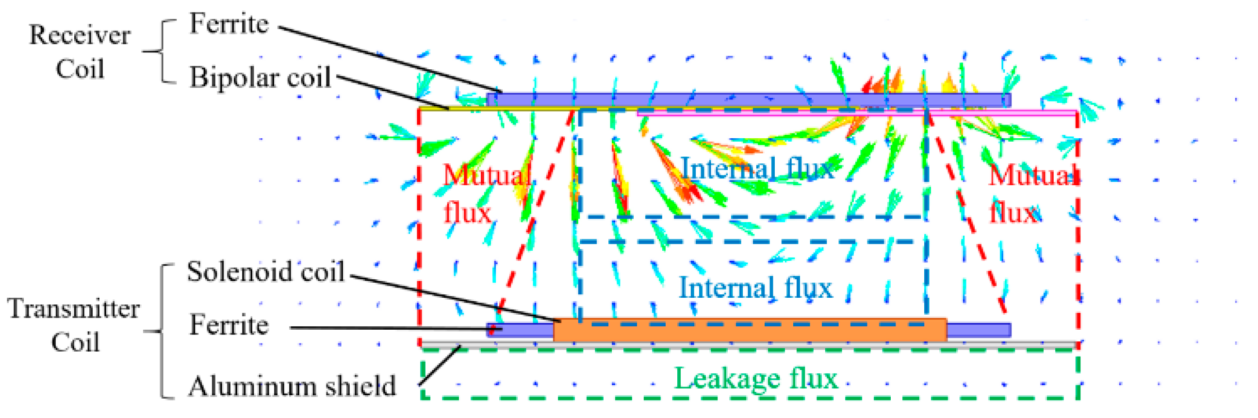
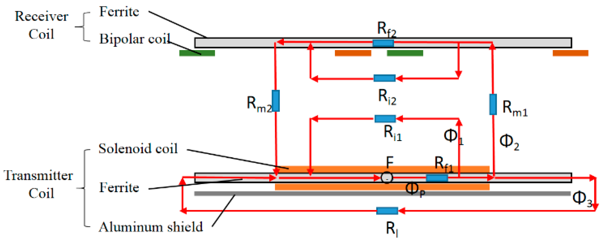
2. Design of Loosely Coupled Transformers

As discussed in previous literature [5,8,9,10,11,12], the solenoid transformer has a high coupling coefficient between primary and secondary side, but it also has high magnetic leakage on the back, so additional shielding is always necessary. In this paper, the solenoid structure is used as the primary side and the bipolar structure as a secondary side. An aluminum plate is placed behind the primary coil to shield the leakage flux. The proposed transformer structure is shown in Figure 5. Position (x = 0, y = 0) is the aligned position between the transmitter and receiver.
A typical flux distribution of the proposed transformer structure is shown in Figure 6. The total flux concerns the internal leakage flux, external leakage flux and mutual flux. The corresponding equivalent magnetic reluctance network is analyzed in Figure 7. The primary structure with excitation winding is modeled as a mmf (magnetic motive force) source. Each magnetic flux path is modelled as a magnetic reluctance, both in the core and in the air. Rf1 and Rf2 are the internal resistances of the ferrite.
According to the equivalent magnetic circuit model,
F ϕ P · R f 1 = ϕ 1 · R i = ϕ 2 · ( R m 1 + R f 2 / / R i 2 + R m 2 ) = ϕ 3 · R l
ϕ P = ϕ 1 + ϕ 2 + ϕ 3
The coupling coefficient between transmitter and receiver is:
k = ϕ 2 ϕ P = 1 R m 1 + R f 2 / / R i 2 + R m 2 1 R i + 1 R m 1 + R f 2 / / R i 2 + R m 2 + 1 R l = 1 ( R m 1 + R f 2 / / R i 2 + R m 2 ) · ( 1 R i + 1 R l ) + 1
As displacement occurs in the +x direction, magnetic resistance Rm1 increases while Rm2 decreases, the variation in coupling coefficients in two receiver coils compensate with each other, and the overall coupling coefficient changes slowly. This is also the case when the displacement occurs in the −x direction. As the displacement increases in the y axis, both Rm1 and Rm2 increase. The overall coupling coefficient decreases correspondingly.
Given fixed design parameters as shown in Figure 8, the coupling coefficient values are calculated in FEM (finite element method) simulations. The variation of coupling coefficient with displacement in x axis is shown in Figure 9. As displacement occurs in the x axis, the coupling coefficient k12 increases while k13 decreases. When the displacement reaches a certain value, k13 starts to increase and k12 starts to go down.
The FEM-based analysis in terms of misalignment tolerance is shown in Figure 10. The misalignment tolerance of the proposed coupler structure has been compared with circular, rectangular, “DD”, bipolar and solenoid structures, based on FEM analysis. The comparison is shown in Table 1. The proposed coupling structure in this paper outperforms the other typical couplers in comprehensive evaluation.

3. Heterogeneous Compensation Network

It has been discussed in previous literature that the S-S (series-series) compensation network features constant current output while the S-LCL compensation network (which adopts series compensation topology on primary side and LCL compensation topology on secondary side) features constant voltage output [13]. As the charging profile of a battery is composed of a constant current phase followed by constant voltage phase, it is straightforward to try to combine the output characteristics of S-S and S-LCL compensation network to fit into the charging curve of the battery. The desired compensation network should satisfy the requirements of a battery, and switch between constant current mode and constant voltage mode. The proposed compensation topology in this paper utilizes the output characteristics of S-S and S-LCL compensation networks, and as the charging process goes on, the system switches between different output modes.

3.1. Basic Principles

The proposed heterogeneous system is shown in Figure 11. A series-resonant full-bridge inverter is implemented as an AC source on the primary side. The secondary side consists of two decoupled coils; each connects with its own compensation network and rectifier, and the two networks are connected in parallel to the load. The output voltage and current signal are collected on the secondary side and transferred to the controller on the primary side.
Lp is the inductance of the primary coil, Ls1 and Ls2 are the inductance of the secondary coil. Cp, Cs1, Cs2 are the compensation capacitors, Cp resonant with Lp, Cs1 resonant with Ls1, Cs2 resonant with Ls2. Rp, Rs1 and Rs2 are the internal resistances of the coils. The battery is modeled as a voltage source E in series with a resistance, and the ESR (equivalent series resistance) of the battery is a function of the battery’s SOC (state of charge).
Figure 11, Uo1 shows the output DC voltage of S branch and Uo2 is the output DC voltage of LCL branch. As the outputs of two rectifier bridges connect in parallel, Uo1 = Uo2 = Uo. The output of the system depends on the comparison of amplitude of Us1 (Us1_m), the amplitude of Us2 (Us2_m), and the battery equivalent voltage (Uo). As two receiver coils are decoupled, the transfer characteristic of each receiver coil is analyzed individually.

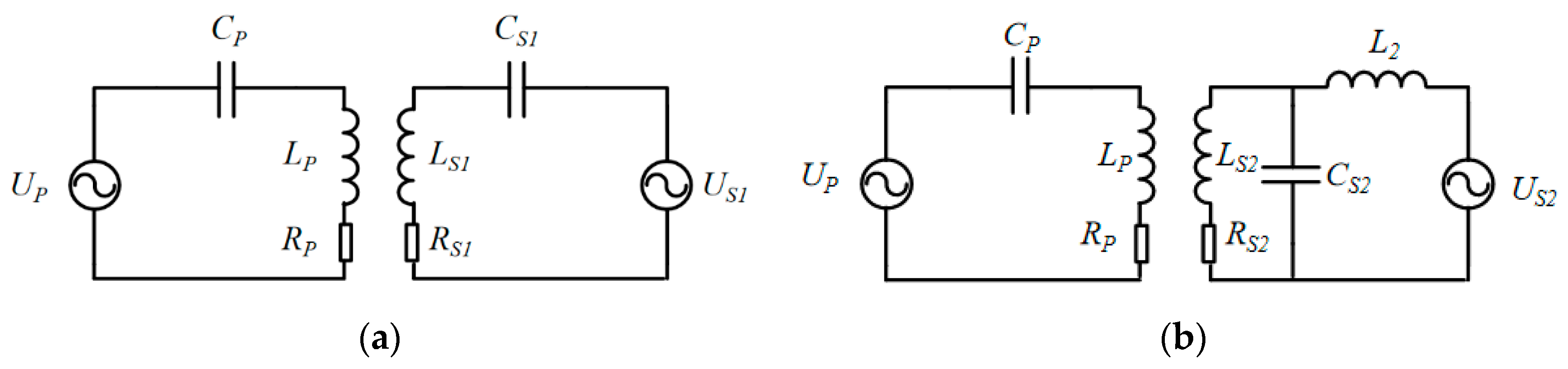
3.1.1. S-S Compensation Topology

The equivalent S-S compensation topology is shown in Figure 12. The rectifier bridge load can be represented using equivalent resistance. At the start if charging process, Uo is so small that it cannot clamp on the rectifier bridge input.
The equivalent impedance of primary and secondary side is,
Z p = 1 j ω C p + j ω L p + R p
Z s 1 = 1 j ω C s 1 + j ω L s 1 + R s 1 + R e q
According to Kirchhoff’s voltage law (KVL) equations,
Z P I P j ω M 1 I S 1 = U p
j ω M 1 I P Z S 1 I S 1 = 0
Solving Equations (6) and (7),
I p = ( R s 1 + R e q ) U p R p ( R s 1 + R e q ) + ( ω M 1 ) 2
I s 1 = j ω M 1 U p R p ( R s 1 + R e q ) + ( ω M 1 ) 2
U s 1 = j ω M 1 · R e q · U p R p ( R s 1 + R e q ) + ( ω M 1 ) 2
I o 1 = I s 1 = j ω M 1 U p R p ( R s 1 + R e q ) + ( ω M 1 ) 2
Assume Rp = Rs1, for different coil internal resistance Rs1, the variation of the effective value of output current IS1 with the equivalent load resistance Req is plotted in Figure 13. As we can see from Figure 14, when the coil resistance is small, the effective value of output current of S-S topology almost remains unchanged with the variation of load resistance. As a matter of fact, the Litz wire used in WPT system is thick and well-fabricated, so the coil resistance is tiny, and the influence of coil resistance on system outputs is minimum. When the coil resistance is tiny, this is a topology with a constant current output feature.

3.1.2. S-LCL Compensation Topology

The equivalent S-LCL compensation topology is shown in Figure 15. The equivalent impedance of the receiver side is:
Z s 2 = R s 2 + j ω L s 2 + R e q + j ω L s 2 1 + j ω C s 2 ( R e q + j ω L s 2 )
The reflected impedance on primary side is:
Z r 2 = ( ω M 2 ) 2 Z s 2 = ( ω M 2 ) 2 R s 2 + j ω L s 2 + R e q + j ω L s 2 1 + j ω C s 2 ( R e q + j ω L s 2 )
The total input impedance is:
Z in = Z p + Z r 2 = j ω L p + 1 j ω C p + R p + ( ω M 2 ) 2 R s 2 + j ω L s 2 + R e q + j ω L s 2 1 + j ω C s 2 ( R e q + j ω L s 2 )
The current in primary loop is:
I P = U p Z i n
Based on Kirchhoff’s voltage law:
Z P I P j ω M 2 I S 2 = U p
j ω M 2 I P Z S 2 I S 2 = 0
To solve Equations (16) and (17), the currents in transmitter and receiver loop are:
I P = Z S 2 U p [ Z P Z S 2 + ( ω M ) 2 ]
I S 2 = j ω M 2 U p [ Z P Z S 2 + ( ω M 2 ) 2 ]
The output current I2 is:
I o 2 = I S 2 1 + j ω C S 2 ( R e q + j ω L S 2 ) = j ω M 2 U p [ Z P Z S 2 + ( ω M 2 ) 2 ] [ 1 + j ω C S 2 ( R e q + j ω L S 2 ) ]
The output voltage Us2 is:
U s 2 = I o 2 · R e q
Assume Rp = Rs2, for different coil internal resistance Rs2, the variation of the effective value of output voltage with the equivalent resistance is plotted in Figure 15. As seen from Figure 16, the output voltage is maintained as almost stable when the load resistance increases above a certain value. With regard to the equivalent resistance of the battery in constant voltage mode, there is a large resistance. The output voltage of the S-LCL topology is regarded as constant voltage.

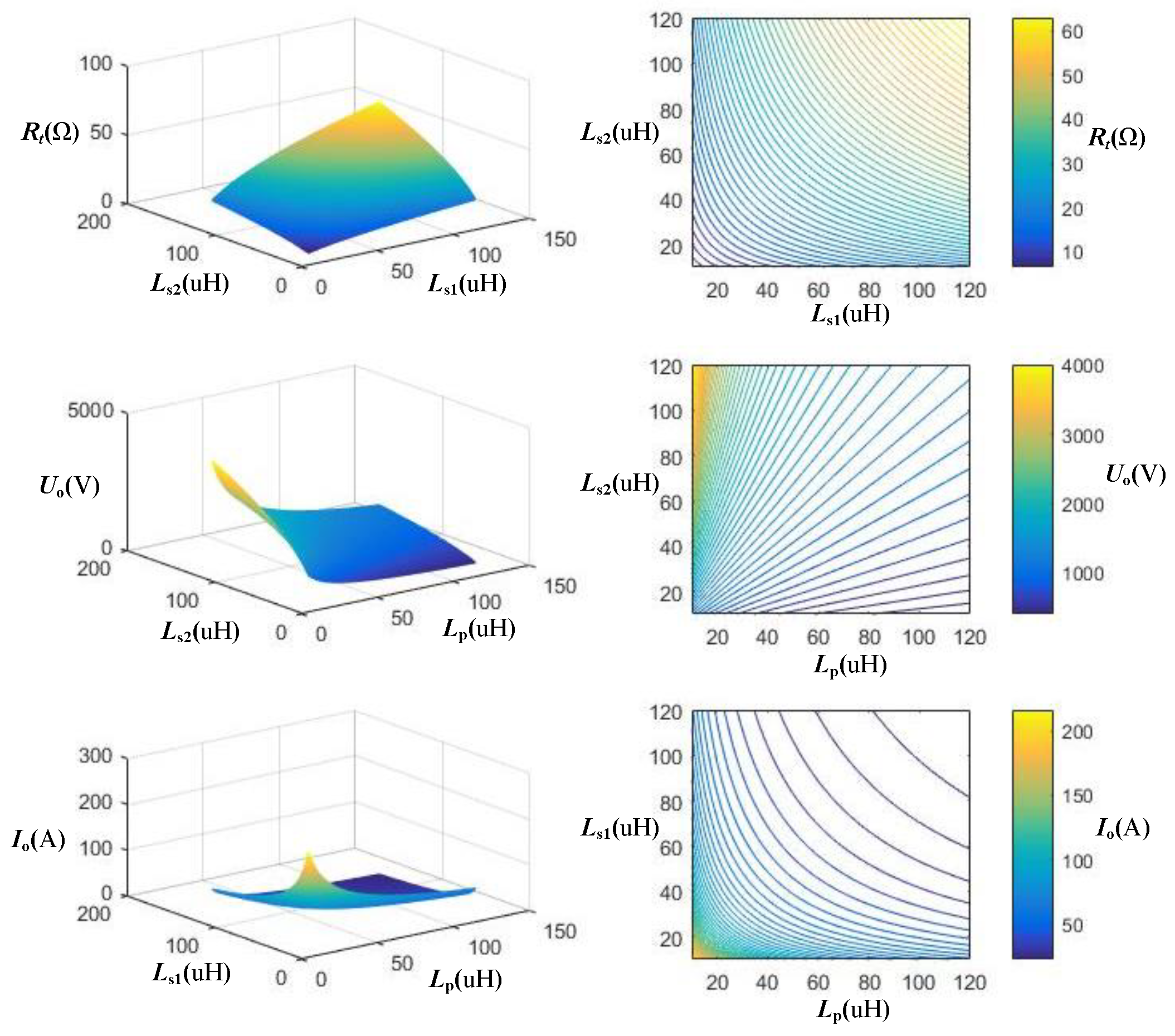
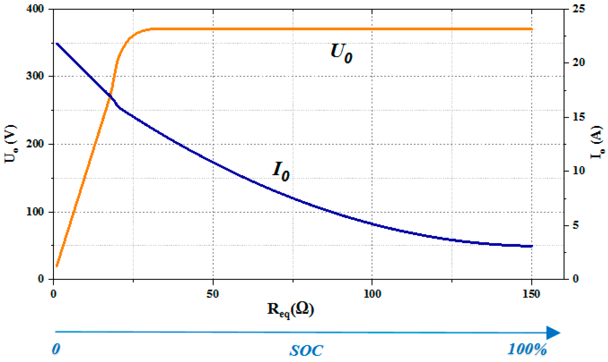
3.2. Transition Point Analysis

At the start of the charging process, the SOC of the battery is small and the equivalent output voltage is low. As SOC increases, the battery’s equivalent output voltage gradually surpasses the output of receiver circuits. Therefore, according to the relative size and relations of US1_m (amplitude of Us1), US2_m (amplitude of Us2) and Uo, there are three charging scenarios:
• Us2_m > Us1_m > Uo
At the beginning of the charging process, when the equivalent voltage of the battery Uo is smaller than the amplitude of Us1 and Us2, both receiver circuits deliver power to the battery. The output current of S branch gradually reduces and the output current LCL branch gradually increases, resulting in a small variation of the total current delivered to the load, and this charging process is regarded as constant current charging.
• Us2_m > Uo > Us1_m
As the SOC of the battery increases, Uo increases and exceeds the amplitude of Us1, the S branch is clamped as the existence of the rectifier bridge. The LCL branch delivers power to the battery.
• Uo > Us2_m > Us1_m
As the SOC further increases, Uo finally exceeds Us1 and Us2, both of the receiver circuits are clamped, and the charging process comes to an end.
The amplitude of output voltage of two receiver circuits are:
U s 1 _ m = 2 j ω M 1 · R e q · U p R p ( R s 1 + R e q ) + ( ω M 1 ) 2
U s 2 _ m = 2 j ω M 2 U p · R e q [ Z P Z S 2 + ( ω M 2 ) 2 ] [ 1 + j ω C S 2 ( R e q + j ω L S 2 ) ]
As the system switches from CC to CV mode, Uo = Us1_m
U o = 2 j ω M 1 · R e q · U p R p ( R s 1 + R e q ) + ( ω M 1 ) 2
As the system switches from CV mode to the end of charging, Uo = Us2_m
U o = 2 j ω M 2 U p · R e q [ Z P Z S 2 + ( ω M 2 ) 2 ] [ 1 + j ω C S 2 ( R e q + j ω L S 2 ) ]
The transition equivalent resistance Rt between CC and CV mode, and transition equivalent resistance Rt between CV and the end of charging can be determined accordingly.
As Req = π2RL/8, and referring to Figure 10,
R L = E + R E S R · I o I o
The one-to-one corresponding relation between the transition ESR = f(SOC) between different charging modes can thus be found.
As for the specific battery chosen, the battery voltage and charging current are measured at the start point, rated point and end point (as shown in Table 2). An ideal voltage source in series with a load resistance is used to represent the battery model.
According to the charging profile of the battery in Table 2, the battery is composed of a 400 V voltage source in series with series-connected resistance. As the charging current decreases from the start point to the rated point, and to the end, the subdivision of the battery’s internal resistance decreases, and the external voltage of the battery increases, which agrees with the charging profile of the battery. The theoretical output curve of the system is plotted in Figure 17.

3.3. Formatting of Mathematical Components

According to the above analysis on two output modes of the topology, the system output voltage and output current as per the transition resistance is expressed as follows:
U o = { j ω M 2 Z S 1 U i R e q 2 [ Z P Z S 1 Z S 2 + ω 2 ( M 1 2 Z S 2 + M 2 2 Z S 1 ) ] j ω M 2 U i R e q 2 [ Z P Z S 2 + ( ω M 2 ) 2 ] [ 1 + j ω C S 2 ( R e q + j ω L S 2 ) ] R e q < R t R e q > R t
I o = { j ω M 2 Z S 1 U i 2 [ Z P Z S 1 Z S 2 + ω 2 ( M 1 2 Z S 2 + M 2 2 Z S 1 ) ] j ω M 2 U i 2 [ Z P Z S 2 + ( ω M 2 ) 2 ] [ 1 + j ω C S 2 ( R e q + j ω L S 2 ) ] R e q < R t R e q > R t
Since the system output transfers from constant current to constant voltage mode, the system output can be written as:
I o = j ω M 2 Z S 1 U i 2 [ Z P Z S 1 Z S 2 + ω 2 ( M 1 2 Z S 2 + M 2 2 Z S 1 ) ] R e q < R t
U o = j ω M 2 U i R e q 2 [ Z P Z S 2 + ( ω M 2 ) 2 ] [ 1 + j ω C S 2 ( R e q + j ω L S 2 ) ] R e q > R t
Usually for a given WPT system, the system resonant frequency is determined to align with commercial regulations. The coupling coefficients k12 and k13 only depend on Lp, Ls1 and Ls2 for a fixed transmission distance. Therefore, according to the specific charging current (IO) and charging voltage (UO) requirement of the battery, the relationship between transition resistance and primary inductance Lp, Ls1 and Ls2 can be derived.
When the internal resistance of the coils is ignored, there is no energy loss in the LCL branch in CC mode, so ZS2 can be ignored, and the system output can be written as:
I o = j Z S 1 U i 2 ω M 2 Z S 1 R e q < R t
U o = j ω M 2 U i R e q 2 [ Z P Z S 2 + ( ω M 2 ) 2 ] [ 1 + j ω C S 2 ( R e q + j ω L S 2 ) ] R e q > R t
The variation of transition resistance, output voltage and output current with inductance Lp, Ls1 and Ls2 are plotted in Figure 18. So for a given UO, IO and Rt, corresponding design values of Lp, Ls1 and Ls2 can be found in Figure 18, which can be used as a reference value when designing the WPT system.
When the internal resistance of the coils is ignored, the original system output expressions, Equations (25) and (26), cannot be simplified. It becomes in-feasible to build a direct mapping relation between UO, IO, Rt and Lp, Ls1, Ls2. Instead, the relationship between UO, IO, Rt and M1, M2 is derived first (As shown in Figure 19), and the values of Lp, Ls1, Ls2 can be obtained, correspondingly.

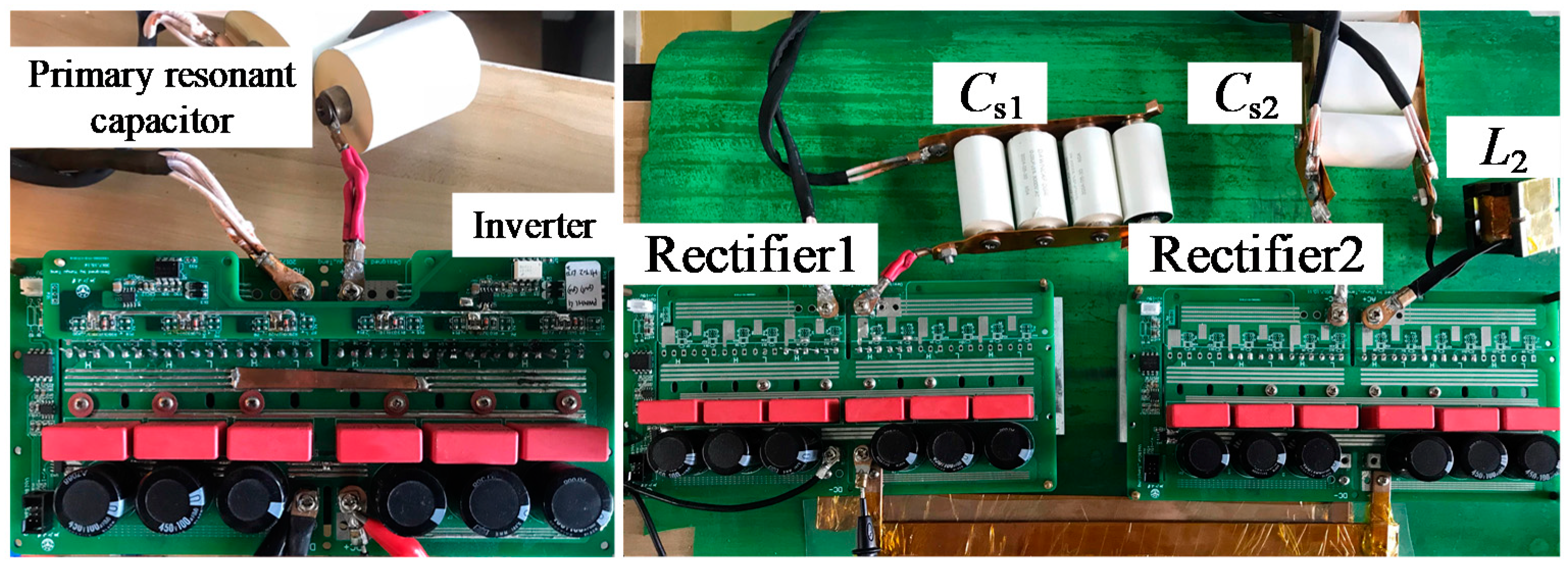
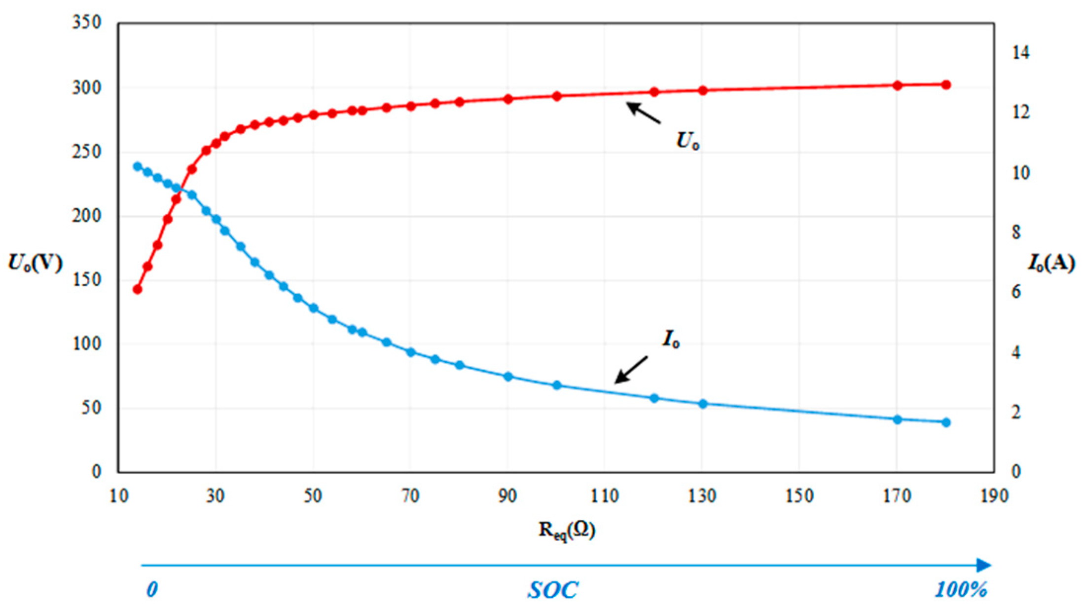
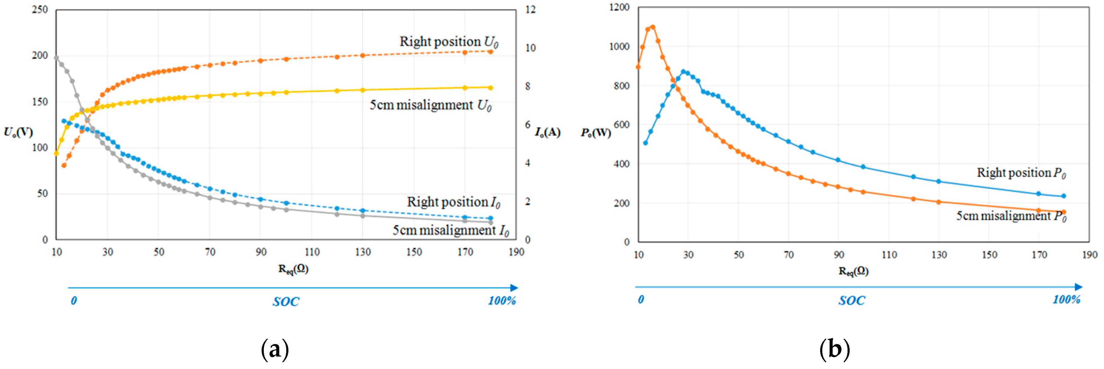
4. Experimental Verification

A 3 kW experimental platform was established to verify the performance of the transformer and topology proposed in this paper, as shown in Figure 20 and Figure 21. The winding uses 0.1 mm × 400 litz wires and the ferrite material is DMR95 with 2500 permeability. The main parameters of the system are shown in Table 3.
As shown in Figure 22, when the system works at constant voltage mode, there is no current output in the series compensated branch, and the system works at S-LCL compensation topology. In constant current mode and the transient process, both compensation topologies provide power to the load simultaneously.
A series of load resistances are used to simulate the resistance variation in a battery charging process, and the system works at open loop status. The variation of output voltage and current with ESR is shown in Figure 23. The system is able to switch between different working modes automatically, and the output characteristics agree with theoretical analysis.
The waveform of voltage output of the inverter and resonant current on primary side is shown in Figure 24. In both constant voltage and constant current mode, the phase of current slightly lags behind the phase of voltage, which ensures the ZVS condition.
The converter waveform on the primary and secondary side on a large time scale is shown in Figure 25b and compared with the simulation results in Figure 25a. As ESR decreases, the system output mode switches from constant current to constant voltage.
As the primary and secondary coils move apart in the y direction, both of the coupling coefficients between two coils on the secondary side and the primary coil decrease. Corresponding system output variations are plotted in Figure 26.
When misalignment occurs in the x axis, the coupling coefficients between secondary coils and primary coil demonstrates different trends of variation. On the one hand, the change of coupling coefficient affects output voltage and current, and on the other hand, the inequality between two coupling coefficients will incur the shift point of the working mode. The system outputs under the right position and 5 cm misalignment are shown in Figure 27. Under the circumstances of 5 cm misalignment, the output current in constant current mode increases while the output voltage in constant voltage mode decreases. Meanwhile, the shift resistance between constant current and constant voltage stages decreases, which will disturb the normal working condition. In real applications, the x direction can be set as the driving direction of the car, so as to make it easier to adjust the misalignment.
The system DC-DC efficiency has been measured at the aligned and misalignment positions (see Figure 28), using a high bandwidth power analyzer (WT1800) with less than 0.1% error. At each position, there is a slight variation in efficiency (1~1.5%) because of the load variations. The measured efficiency was compared with the results in existing literature in Table 4. The proposed structure in this paper is proved to have higher energy efficiency compared to other research results with similar dimensions.

5. Conclusions

This paper presents a novel method of wireless charging to a lithium battery on electric vehicles. A transformer structure using a solenoid structure on the primary side, and a bipolar structure on the secondary side, is proposed. To satisfy the charging requirement of a lithium battery on electric vehicles, a system topology with series compensation on the primary side, and a heterogeneous compensation network on the secondary side, is proposed. This system is able to automatically switch between constant current and constant voltage output mode based on transition resistance, without additional control loops. Theoretical analysis of this heterogeneous topology is presented with explanations, based on the ESR model of the battery. A 3 kW experimental platform is established and the validity of theoretical analysis is confirmed. This proposal offers a new open-loop approach to offer the precise charging curve to lithium batteries without additional control hardware.

Author Contributions

Conceptualization, J.Z., P.Y. and P.C.; methodology, J.Z. and P.Y.; validation, J.Z., P.Y. and K.G.; formal analysis, J.Z. and P.Y.; investigation, K.G. and P.C.; resources, P.C. and Y.Z.; writing—original draft preparation, J.Z. and P.Y.; writing—review and editing, J.Z.; supervision, H.M.; project administration, J.Z. All authors have read and agreed to the published version of the manuscript.

Funding

This research received no external funding.

Conflicts of Interest

The authors declare no conflict of interest.

References

  1. Hui, S.Y.R.; Zhong, W.; Lee, C.K. A Critical Review of Recent Progress in Mid-Range Wireless Power Transfer. IEEE Trans. Power Electron. 2014, 29, 4500–4511. [Google Scholar]
  2. Mi, C.C.; Buja, G.; Choi, S.Y.; Rim, C.T. Modern Advances in Wireless Power Transfer Systems for Roadway Powered Electric Vehicles. IEEE Trans. Ind. Electron. 2016, 63, 6533–6545. [Google Scholar]
  3. Zhang, C.; Lin, D.; Hui, S.Y. Ball-Joint Wireless Power Transfer Systems. IEEE Trans. Power Electron. 2018, 33, 65–72. [Google Scholar]
  4. Zhang, C.; Lin, D.; Tang, N.; Hui, S.Y.R. A Novel Electric Insulation String Structure with High-Voltage Insulation and Wireless Power Transfer Capabilities. IEEE Trans. Power Electron. 2018, 33, 87–96. [Google Scholar]
  5. Tang, Y.; Zhu, F.; Wang, Y.; Ma, H. Design and optimizations of solenoid magnetic structure for inductive power transfer in EV applications. In Proceedings of the 41st Annual Conference of the IEEE Industrial Electronics Society (IECON 2015), Yokohama, Japan, 9–12 November 2015. [Google Scholar]
  6. Hu, S.; Liang, Z.; He, X. Ultracapacitor-battery hybrid energy storage system based on the asymmetric bidirectional Z-source topology for EV. IEEE Trans. Power Electron. 2016, 31, 7489–7498. [Google Scholar]
  7. Hu, S.; Liang, Z.; Fan, D.; He, X. Hybrid Ultracapacitor–Battery Energy Storage System Based on Quasi-Z-source Topology and Enhanced Frequency Dividing Coordinated Control for EV. IEEE Trans. Power Electron. 2016, 31, 7598–7610. [Google Scholar]
  8. Budhia, M.; Covic, G.A.; Boys, J.T. Design and Optimization of Circular Magnetic Structures for Lumped Inductive Power Transfer Systems. IEEE Trans. Power Electron. 2011, 26, 30963108. [Google Scholar]
  9. Kim, J.; Kim, J.J.; Kong, S.; Kim, H.; Suh, I.-S.; Suh, N.P.; Cho, D.-H.; Kim, J.; Ahn, S. Coil Design and Shielding Methods for a Magnetic Resonant Wireless Power Transfer System. Proc. IEEE. 2013, 101, 1332–1342. [Google Scholar]
  10. Budhia, M.; Boys, J.T.; Coyic, G.A.; Huang, C.Y. Development of a single-sided flux vehicle IPT charging systems. IEEE Trans. Ind. Electron. 2013, 60, 318–328. [Google Scholar]
  11. Budhia, M.; Covic, G.; Boys, J. A new IPT magnetic coupler for electric vehicle charging systems. In Proceedings of the 36th Annual Conference of IEEE Industrial Electronics Society (IECON 2010), Glendale, AZ, USA, 7–10 November 2010. [Google Scholar]
  12. Nagatsuka, Y.; Ehara, N.; Kaneko, Y.; Abe, S.; Yasuda, T. Compact contactless power transfer system for electric vehicles. In Proceedings of the 2010 International Power Electronics Conference—ECCE ASIA, Sapporo, Japan, 21–24 June 2010. [Google Scholar]
  13. Cao, P.; Tang, Y.; Zhu, F.; Zhang, Z.; Zhou, J.; Bai, Z.; Ma, H. An IPT System with Constant Current and Constant Voltage Output Features for EV Charging. In Proceedings of the 44th Annual Conference of the IEEE Industrial Electronics Society (IECON 2018), Washington, DC, USA, 21–23 October 2018. [Google Scholar]
  14. Li, Z.; Zhu, C.; Jiang, J.; Song, K.; Wei, G. A 3-kW Wireless Power Transfer System for Sightseeing Car Supercapacitor Charge. IEEE Trans. Power Electron. 2016, 32, 3301–3316. [Google Scholar]
  15. Qu, X.; Han, H.; Wong, S.-C.; Tse, C.K.; Chen, W. Hybrid IPT Topologies With Constant Current or Constant Voltage Output for Battery Charging Applications. IEEE Trans. Power Electron. 2015, 30, 6329–6337. [Google Scholar]
  16. Mai, R.; Chen, Y.; Li, Y.; Zhang, Y.; Cao, G.; He, Z. Inductive Power Transfer for Massive Electric Bicycles Charging Based on Hybrid Topology Switching With a Single Inverter. IEEE Trans. Power Electron. 2017, 32, 5897–5906. [Google Scholar]
  17. Li, Y.; Xu, Q.; Lin, T.; Hu, J.; He, Z.; Mai, R. Analysis and Design of Load-Independent Output Current or Output Voltage of a Three-Coil Wireless Power Transfer System. IEEE Trans. Transp. Electrif. 2018, 4, 364–375. [Google Scholar]
  18. Chen, Y.; Yang, B.; Kou, Z.; He, Z.; Cao, G.; Mai, R. Hybrid and Reconfigurable IPT Systems With High-Misalignment Tolerance for Constant-Current and Constant-Voltage Battery Charging. IEEE Trans. Power Electron. 2018, 33, 8259–8269. [Google Scholar]
  19. Kim, M.; Joo, D.-M.; Lee, B.K.; Woo, D.-G. Design and control of inductive power transfer system for electric vehicles considering wide variation of output voltage and coupling coefficient. In Proceedings of the 2017 IEEE Applied Power Electronics Conference and Exposition (APEC), Tampa, FL, USA, 26–30 March 2017. [Google Scholar]
  20. Berger, A.; Agostinelli, M.; Vesti, S.; Oliver, J.A.; Cobos, J.A.; Huemer, M. A Wireless Charging System Applying Phase-Shift and Amplitude Control to Maximize Efficiency and Extractable Power. IEEE Trans. Power Electron. 2015, 30, 6338–6348. [Google Scholar]
  21. Matysik, J.T. The Current and Voltage Phase Shift Regulation in Resonant Converters with Integration Control. IEEE Trans. Ind. Electron. 2007, 54, 1240–1242. [Google Scholar]
  22. Wang, C.-S.; Covic, G.A.; Stielau, O.H. Power Transfer Capability and Bifurcation Phenomena of Loosely Coupled Inductive Power Transfer Systems. IEEE Trans. Ind. Electron. 2004, 51, 148–157. [Google Scholar]
  23. Zhong, W.; Hui, S.Y. Reconfigurable Wireless Power Transfer Systems with High Energy Efficiency Over Wide Load Range. IEEE Trans. Power Electron. 2018, 33, 6379–6390. [Google Scholar]
  24. Yang, Y.; Zhong, W.; Kiratipongvoot, S.; Tan, S.-C.; Hui, S.Y.R. Dynamic Improvement of Series–Series Compensated Wireless Power Transfer Systems Using Discrete Sliding Mode Control. IEEE Trans. Power Electron. 2018, 33, 6351–6360. [Google Scholar]
  25. Qu, X.; Jing, Y.; Han, H.; Wong, S.-C.; Tse, C.K. Higher Order Compensation for Inductive-Power-Transfer Converters With Constant-Voltage or Constant-Current Output Combating Transformer Parameter Constraints. IEEE Trans. Power Electron. 2017, 32, 394–405. [Google Scholar]
  26. Zaheer, A.; Hao, H.; Covic, G.A.; Kacprzak, D. Investigation of Multiple Decoupled Coil Primary Pad Topologies in Lumped IPT Systems for Interoperable Electric Vehicle Charging. IEEE Trans. Power Electron. 2015, 30, 1937–1955. [Google Scholar]
  27. Bosshard, R.; Kolar, J.W. All-SiC 9.5 kW/dm3On-Board Power Electronics for 50 kW/85 kHz Automotive IPT System. IEEE J. Emerg. Sel. Top. Power Electron. 2017, 5, 419–431. [Google Scholar]
  28. Deng, J.; Li, W.; Nguyen, T.D.; Li, S.; Mi, C.C. Compact and Efficient Bipolar Coupler for Wireless Power Chargers: Design and Analysis. IEEE Trans. Power Electron. 2015, 30, 6130–6140. [Google Scholar]
Figure 1. Typical charging curve of a lithium battery.
Electronics 09 01978 g001
Figure 2. Typical diagram of inductive charging system.
Electronics 09 01978 g002
Figure 3. Typical transformer structures of the WPT system.
Electronics 09 01978 g003
Figure 4. Normalized voltage-frequency response surface of a typical WPT system (λ is the coupling factor, which indicates the tightness of coupling between the transmitter and receiver, and ζ is the detuning factor, which represents the degree to which the working frequency deviates from the resonant frequency).
Electronics 09 01978 g004
Figure 5. Proposed transformer structure.
Electronics 09 01978 g005
Figure 6. Flux distribution of the proposed transformer structure.
Electronics 09 01978 g006
Figure 7. Equivalent magnetic reluctance network.
Electronics 09 01978 g007
Figure 8. Design parameters of the proposed transformer structure.
Electronics 09 01978 g008
Figure 9. Variation of total coupling coefficient: (a) k12 with displacement; (b) k13 with displacement.
Electronics 09 01978 g009
Figure 10. FEM simulation misalignment positions alongside ferrite direction: (a) aligned position; (b) 80 mm; (c) 150 mm; (d) 300 mm.
Electronics 09 01978 g010
Figure 11. Schematic diagram of the proposed system.
Electronics 09 01978 g011
Figure 12. Equivalent S-S compensation topology.
Electronics 09 01978 g012
Figure 13. Compensation networks of (a) S-S; (b) S-LCL.
Electronics 09 01978 g013
Figure 14. Variation of output current with equivalent resistance.
Electronics 09 01978 g014
Figure 15. Equivalent S-LCL compensation topology.
Electronics 09 01978 g015
Figure 16. Equivalent S-LCL compensation topology.
Electronics 09 01978 g016
Figure 17. Theoretical output curves of system.
Electronics 09 01978 g017
Figure 18. Contour map of system parameters (UO, IO, Rt and Lp, Ls1, Ls2).
Electronics 09 01978 g018
Figure 19. Contour map of system parameters (UO, IO, Rt and M1, M2).
Electronics 09 01978 g019
Figure 20. Experiment platform.
Electronics 09 01978 g020
Figure 21. Transformer structure.
Electronics 09 01978 g021
Figure 22. Current distribution: (a) constant voltage mode; (b) transient process; (c) constant current mode.
Electronics 09 01978 g022
Figure 23. System output curves in open loop.
Electronics 09 01978 g023
Figure 24. Zero voltage switching (ZVS) waveform with (a) 14 Ω load resistance; (b) 180 Ω load resistance.
Electronics 09 01978 g024
Figure 25. Converter waveform on primary and secondary side (a) simulated; (b) experimental.
Electronics 09 01978 g025
Figure 26. Variation with equivalent resistance at different displacements in y axis: (a) output voltage and current; (b) system output power.
Electronics 09 01978 g026
Figure 27. Variation with equivalent resistance at different displacements in the x axis: (a) output voltage and current; (b) system output power.
Electronics 09 01978 g027
Figure 28. System efficiency at aligned and misaligned positions.
Electronics 09 01978 g028
Table 1. Comparison with different coupling structures.
StructureCouplingCostMisalignment ToleranceSystem ComplexityElectro-Magnetic Radiation
CircularLowLowLowLowHigh
RectangularLowLowMiddleLowHigh
DDMiddleMiddleMiddleMiddleLow
DDQ 1HighHighHighHighLow
BipolarHighHighHighHighLow
SolenoidHighMiddleMiddleLowHigh
ProposedHighMiddleHighMiddleLow(shielded)
1 An additional circular coil added on DD structure.
Table 2. Battery charging profile.
StartRated PointEnd
Battery Voltage (V)200380~400
Charging Current (A)159Small current
Table 3. System key parameters.
SymbolVariableValue
fSystem resonant frequency85 kHz
LpSelf-inductance of primary coil234 μH
Ls1Self-inductance of secondary coil1106 μH
Ls2Self-inductance of secondary coil212 μH
L2LCL network resonant inductance12 μH
k12Coupling coefficient between primary coil and secondary coil10.17
k13Coupling coefficient between primary coil and secondary coil20.17
CpResonant capacitance on primary side0.014 μF
Cs1Resonant capacitance on secondary side 10.03 μF
Cs2Resonant capacitance on secondary side 20.276 μF
Table 4. System output parameters and comparison with existing literature.
Dimensions (mm) × gap (mm)Misalignment (mm)Coupling CoefficientEfficiency (Aligned)Efficiency (300 mm Misalignment)
Proposed600 × 600 × 200+/−3000.35–0.295.2% (~94.2%)92.2% (~90.7%)
The University of Auckland [26]775 × 485 × 200+/−2000.3–0.1590%86%
ETH (Swiss Federal Institute of Technology Zurich) [27]760 × 410 × 160+/−1500.23–0.1596%92%
San Diego State University [28]600 × 600 × 150+/−2000.3–0.1495%92%
Publisher’s Note: MDPI stays neutral with regard to jurisdictional claims in published maps and institutional affiliations.

