On the Mediation Price War of 5G Providers

Abstract

Virtualization guarantees that, moving toward 5G, online services will be versatile and the creation of those will be quick, satisfying the interest of end-clients to a higher degree than what is plausible today. Telcos, cloud administrators, and online application suppliers will unite for conveying those services to clients around the world. Thus, in order to help their portability, or the simple geographic range of the offered application, the business arrangements among the actors must scale over numerous domains and a guaranteed nature of joint effort among different stakeholders is important. Therefore, the vision of the 5G environment is majorly established on the federation of these partners in which they can consistently strive towards the objective of making reliable resource slices and deploying applications within for a maximal geographic reach of clients. In this environment, business perspectives will significantly impact the technical capacity of the system: the business arrangements of the providers will innately decide the accessibility and the end-client costs of certain services. In this work, we model the business relations of infrastructure providers as a variation of network formation games. We infer conditions under which the current transit-peering structure of network providers stays unblemished, and we also draw the specifics of an envisioned setup in which providers create business links among each other starting with a clean slate.

1. Introduction

Keeping the activity of the autonomous systems manageable in the present Internet has a cost of lessening the degree of their interoperability to best effort. Subsequently, when one considers making services that reach over numerous administrative domains, they cannot guarantee Quality of Service (QoS). The 5G vision anticipates online services to be more advanced [1] than the present ones for which infrastructure providers ensure end-to-end QoS in network slices [2] with small delay and large bandwidth capacity. Moreover, with the appearance of virtualization both in compute and network technologies, quicker service creation is feasible and the reconfiguration of those can be more versatile, bringing about a totally novel life-cycle management approach contrasted with what the present standard is [3]. The idea of elastic resource slicing [4] is the key empowering ingredient for this [5], and when different providers partake in making a resource slice, comparably exacting commitment to QoS assurance is required from all members [4,6].

1.1. Motivation and Goal

The locality of clients is one of the most significant driving variables of the birth of multi-provider resource slices [4,6]. Connectivity requisites of services naturally characterize the potential set of qualified networks for the resource slice: the required latency guarantees of given Virtual Network Functions (VNFs) decide whether it should be to the cloud or to an edge cloud (or fog) near the clients, and in which one they can be sent for conveying QoS [7]. One of the other significant characteristics is cost: when QoS necessities permit, it can drive the requirement for multi-domain resource slice creation [8]. Luckily, Network Function Virtualization (NFV) makes it conceivable to make adaptable services in the form of Service Function Chains (SFC) of VNFs when the suitable resource slice has been made.

Roused by these elements, we anticipate that 5G framework actors will work together in alliances. In order to have the option to offer locality-aware services for their clients around the world, they will utilize the compute and network assets of any of their fellow suppliers [4,6]. However, before committed resource slices are provisioned crossing over different providers’ authoritative domains, business arrangements must be set up between partners, e.g., on cost and QoS assurance designated to the resource slice [9,10]. For the end-to-end QoS capabilities of a resource slice that numerous providers partake in, dispersed arrangements and consistently kept up business connections may be vital among the stakeholders [11].

We believe that the current Internet pricing models based on transit and peering cost decisions will be challenged due to the change of the service obtained in the future. More specifically, as long as the service is mere connectivity, aggregation and hiding the connectivity topology are substantial. Therefore, a transit provider providing default access to the rest of the Internet is sufficient unless serious bottlenecks are detected. However, in envisioned 5G services connectivity interleaves with compute services where proximity becomes a key asset. Therefore, address reachability information may be complemented with cloud availability and capability information on considering edge deployments. If incumbent transit providers, who do not necessarily possess (deep) edge clouds, are not willing to proxy, process, and forward network slice orchestration requests, then providers must establish bi-, or multilateral contracts similar to Internet peering, which comes with extra operational costs. We investigate the rationale for all operator players to evolve services from connectivity-only to 5G network slicing via their existing transit and peering business relationships, i.e., under what mediation pricing strategy incumbent transit providers can enter the 5G slicing market to prevent lower tier providers to enter into bilateral direct business contracts. In this work, we research how the organization of business relations may advance in the reign of 5G: will it follow the geography of transit and peering relations of the Web today [12] or will new business relations be set up between neighboring or far off providers correspondingly to ISPs’ peering arrangements? We propose a model that grasps the benefits and costs of additional business relationships, and we give analytical and numerical evaluations that answer this question.

1.2. Related Work

To the best of our knowledge, currently there are no available publications that would investigate the pricing of multi-actor resource slices. We have also not discovered any work that researched the particular cost factor due to keeping up business relations or the cost of interceding business agreements to this end in a multi-provider arrangement. Therefore, here we summarize related work that connects to our domain of research, and we make the connection explicit by comparing their results to ours. We group the collected research papers into three categories: resource pricing in the cloud, network formation games, Internet connectivity prices, and agreements.

1.2.1. Resource Pricing in the Cloud

The research in [13] focused on mobile cloud computing, i.e., the integration of cloud computing into a mobile ecosystem, thus enabling on-demand and elastic resource utilization for mobile users. The article, however, emphasized that further work was required to explore the trade-off between the benefits of uploading tasks and the price that mobile users must pay for the same.

The overview in [14] summarized pricing models for cloud computing. The vast majority of the gathered research papers within propose the utilization of dynamic prices, as it serves the provider’s benefit when the following two product attributes exist together: first, the item lapses at a point in time; second, there is a fixed limit on the amount of products and it is exorbitant to be expanded. The term cloud networking is perceived in a multi-administration situation in which network and cloud domains interface with one another. All things considered, the comprehensive assortment of related work introduced in [14] does exclude research results that tackle both different suppliers and different resource types, i.e., compute and network resources, to sell.

Related to pricing aspects of 5G network slices, in [1], the authors proposed a model for network slicing under the control of a single infrastructure provider: they introduced an analytical model for admission control of slicing-capable 5G networks. Furthermore, they also proposed a method for optimizing the revenue of the infrastructure provider.

In [15], the authors tackled a problem seemingly similar to ours with the same tool set: resource allocation for network slices among multi-tier stakeholders in a Stackelberg game. The problem they modeled, however, covered wireless channel allocation of access providers, i.e., leaders, and user equipment subscriptions, i.e., followers. The payoff models were built such that convex optimization problems arose, i.e., followers set their demand independently from each other, but in response to the prices advertised by the leaders; leaders determined their prices in an iterative process by giving best response to others’ prices, but independent of the price to pay towards the backhaul providers. The latter were also part of the analysis, i.e., determining the price of the bandwidth to sell to access providers, but the backhaul providers were not part of the Stackelberg game.

The authors of [8,10] argued that future online services would be provisioned over the federation of infrastructure providers for economic reasons: for effective usage of resources and for a wide geographic reach of customers. They modeled the infrastructure providers that compete among themselves for the customers, and shape their business offerings with profit maximization in mind. They showed that customers face a hard problem if they want to meet both their technical and business needs, let alone minimizing costs. They also derived the best pricing strategies that the providers should follow given their expectation about customers’ demand. As the main result, the authors showed that equilibrium prices and the attainable income strongly depend on the provider’s location within the network.

In all of this related work, the optimal pricing scheme for compute and/or network resources was sought, mostly in a single-provider multi-user setting. In contrast to this work, our endeavor is to model the business costs of interaction between providers. As such, our assumed setup is inherently multi-provider multi-user, and the end user prices are only indirectly addressed in our analysis.

1.2.2. Network Formation Models

The second area of the related work is best described by network formation models, inspired by the stability of the Internet despite its sheer size. Large computer networks, such as the Internet, are built, operated, and used by a large number of diverse and competitive entities. In light of these competing forces, it is surprising how efficient these networks are. An exciting challenge in the area of algorithmic game theory is to understand the success of these networks in game theoretic terms: network formation games are widely used to investigate the principles of interaction that lead selfish participants to form efficient networks.

Fabrikant et al. presented the network formation game that modeled the dynamic building process of networks by economically selfish nodes without any central coordination [16]. In their model, nodes pay for the connections that they set up, and pull advantage from the short routes to all fellow nodes. The authors examined the Nash equilibria of the game, and inferred results about the “price of anarchy”, i.e., the overall loss due to the absence of coordination.

Corbo et al. contemplated a network formation game where connections required the assent of the two nodes and were negotiated reciprocally [17]. The authors contrasted these networks with those produced by the prior model of [16] in which connections were created unilaterally. Their observations exhibited that the average price of anarchy was better in the reciprocal network formation game than in the one-sided game for little connection costs, however worse as connections become more costly.

The book chapter [18] investigated various different network formation games regarding the loss that comes from game theoretical selfishness.

Another work that handles reciprocally concurred agreements was introduced in [19]: cost was caused to a node from four sources: (1) routing traffic; (2) keeping up connections to different nodes; (3) getting disconnected from nodes it wished to reach; and (4) installments made to different nodes. The authors studied the game in context of the idea of pairwise stability. The distinction contrasted with our work is that our model records for the “routing” term as income source, rather than making it a cost-expanding term.

All these network formation models and the games defined on them considered a flat, single-layer topology in which nodes, i.e., network providers, are homogeneous. In this aspect, our assumption about the players is different: as in the related work on the economics of the Internet, discussed in the following, we consider a tiered setup of nodes in which upper layer network providers are significantly larger in terms of infrastructure and end user base than lower layer network providers. This context makes the network formation game entirely different.

1.2.3. Internet Economics

The authors of [20] focused on the Internet topology as they analyzed the interactions of Internet Service Providers (ISPs) at different levels: (1) when they compete directly for customers, (2) when they belong to different levels of the hierarchy, and (3) when they try to bypass a section of the hierarchy. The paper examined the existence of equilibrium strategies through a Stackelberg game [21] along the ISPs’ tiered hierarchy. The authors derived conclusions on the possible evolution of the Internet topology focusing on local ISPs, anticipating that ISPs in each region would set similar prices and provide similar QoS levels.

Dhamdhere et al. investigated how the Internet ecosystem evolved from a multi-tier hierarchy, built mostly with transit (customer-provider) links, to a dense mesh, formed with mostly peering links [22]. They studied this evolutionary transition with an agent-based network formation model that captured key aspects of the inter-domain ecosystem, e.g., traffic flow and routing, provider and peer selection strategies, geographical constraints, and the economics of transit and peering interconnections. Their model predicted several differences between the Hierarchical Internet and the Flat Internet in terms of topological structure, path lengths, and the profitability of transit providers.

The same authors published an agent-based network formation model for the Internet at the Autonomous System (AS) level in [23]: ASes act in a myopic and decentralized manner to optimize a cost-related fitness function, capturing key factors that affect the network formation dynamics, such as highly skewed traffic matrix, policy-based routing, geographic co-location constraints, and the costs of transit/peering agreements. As opposed to analytic game-theoretic models, which focus on proving the existence of equilibria, this was a computational model that simulated the network formation process and allowed to actually compute distinct equilibria (i.e., networks) and to also examine the behavior of sample paths that do not converge. They found that such oscillatory sample paths occur in about 10% of the runs, and they always involved Tier-1 ASes, resembling the Tier-1 peering disputes often seen in practice.

In another work [24], the same authors investigated why many transit providers apply open peering strategy. They also examined the impact of an Open peering variant that requires some coordination among providers.

These selected papers from the body of research on Internet economics focused on the hidden reasons of the Internet topology evolution, specifically the decade-long investigation on transit vs. peering relations in the Internet. In the late 2000s, peering links between ISPs started to form in great numbers. This phenomenon inspired the researchers, and several of them applied game theoretical methodologies to model and explain this prominent trend. Although the methodology we apply is similar, our focus is not on the exchanged traffic between ISPs, rather on the multi-provider resource slice creation between infrastructure providers that might operate at remote geographic location far from each other. However, the sense of end-to-end connectivity is also found in our research domain, only not in the classical user plane sense, rather as business relationships.

1.3. Contributions

We formalize the development of business relations as a network formation game in an envisioned multi-provider multi-user setup, where resource slices are created for users that might be located out of the direct reach of their provider, thus the slices to be created are possible overarching multiple providers, comprising compute and network resources of remote providers. We present the interplay between two contradicting effects. First, we represent a creation and upkeep cost of business connections that are paid as a provider builds up contracts with a number of fellow actors. Second, we introduce the notion of mediation prices, collected by middleman actors; these providers who have direct links to other providers that are not directly interconnected with a business link, but want to initiate the creation of a resource slice with each other, with the help of the middleman.

We study this game from the perspective of profit-oriented 5G infrastructure providers in order to characterize this business trade-off of those opposing forces. Our contributions in this paper consist of (i) analytic conditions on these pricing factors for a stable business relationships topology, (ii) formulas that describe the expected middleman prices if providers start making business relationships from scratch. For the first point, we write a formal condition on the highest price that middlemen can ask, at which the actors do not have any incentives to create new business links. Furthermore, by numerical simulations, we depict the complex phenomenon which is produced by the link creation and middleman prices, the demand for resource slices, and the business topology. This paper extends our early results published in [11] by interpreting the stakeholders’ interactions as a Stackelberg game of Bertrand competitions and by describing the equilibrium point of this business network formation game. The numerical analysis is also significantly extended with a two-phase simulation model and the discussion of the new results.

As analytical results, we prove that high tier providers have a motivating force to keep their broker costs low in order to preserve their place in the ecosystem, and in an alternative setup with business links being created starting from a clean slate situation, we determine the equilibrium prices with parameterized formulas. With the numerical results, we show the interesting interplay of the number of created links and the attached costs, in addition to the distribution of business path lengths that arise in stable setups.

The rest of the paper is organized as follows. In Section 2, we define our business network model and the trade-off we study in detail; then, we formalize the model as a network formation game, and derive analytic results on equilibrium conditions. In Section 3, we describe our numerical analysis and show simulation results in a general setting. The results are discussed in Section 4. Finally, we conclude our work in Section 5 and have an outlook on future work.

2. Method: Business Network Model and Formation Game

In this section, we present the model and the analytical results we derive thereof. Our model is built in the intersection of the three areas of related work discussed in Section 1.2: we tackle the pricing scheme of 5G cloud and network infrastructure providers that drives the evolution of their business topology with the methodology and tool set of network formation games. Furthermore, in our opinion, the arrangement of future 5G business networks is exceptionally reliant of, and, in this way, will be at first dependent on the current Web topology. Thus, we expect a layered structure following the present Internet transit and peering relations as our underlying topology model to proceed with the assessment on how the new 5G environment may adjust the initial setup. We showcase the fundamental trade-off regarding expenses of keeping up business relations, and the cost of business mediators.

2.1. Graph Model of Business Relationships

Figure 1 shows instances of our graph model of 5G providers. In this model, vertices stand for (i) network providers (likewise offering computing services) and (ii) Service Access Points (SAPs), which are reaching points of end-clients. Edges represent business connections, which, in the underlying stage can be either (i) transit relations (depicted by solid lines in the figure) or (ii) peering relations (depicted by dashed lines) between nodes. The locality of clients and delay-critical services are among the most significant driving components of multi-provider setups; accordingly, we portrayed SAPs only at Level 3 providers as those offer access service to end-clients [25]. This is notwithstanding that in our vision all network providers are expected to become 5G cloud operators as well [4,6].

In the center of our model are such multi-domain services in which the end-clients of the service are clients of provider A, but they really utilize the service inside the access domain of provider B. In this situation, provider A purchases a resource slice from provider B (and perhaps from different providers interconnecting providers A and B). We model these business arrangements as paths in the graph model associating two nodes: the purchaser of the service is essentially the customer-facing provider, while the seller of the service is the provider in whose domain end-clients currently utilize the service. The delay-critical service is subsequently placed at the vendor provider’s premises near the current SAP of the end-client. The service’s descriptive characteristics, e.g., computing needs, explicitly stating VNFs to onboard that comprise the service, network QoS to the SAP, and so forth, should be satisfied and paid for by the purchaser provider. In this multi-provider arrangement, we investigate the development of business relations: we do not handle the pricing of services or that of the resource slices, this study is limited to the valuation of inter-provider organizational possibilities.

2.2. Cost of Business Relations and Price of Middlemen

Deploying a service into the resource slice that is mounted on another provider(s) infrastructure requires prior negotiations and a pre-built business link or path among the partners, similarly to the network formation models, e.g., in [19]. As depicted in Section 1, we assume that two opposing effects decide how these arrangements are made: either by a direct business made between the two parties, or through a chain of agents that relay between the seller and purchaser providers. In the second case, the base cost of the resource slice is supplemented by the business relay cost of the interconnecting providers. The length of the chain of mediating providers equals to the number of hops on the path between the two providers in our graph model. Alternatively, each extra immediate business connection between providers incurs an expense at the two players: setting up and keeping up business contracts have their expenses. The trade-off situation is clear: while edges increment the general managerial expenses, barring mediators from setting up resource slices in a remote operator’s infrastructure saves cost. Compared to the classical network formation games [16,17,18], the utility of being strongly connected to other nodes there, is, in our case, translated to fewer middlemen to pay for mediating the business between remote nodes.

Figure 1 showcases the business connection between a chosen pair of SAPs in an underlying layered graph model. The path traverses the transit links towards the highest level of the tiered structure of providers. Nevertheless, another business interconnection can be shaped by building up business associations between any two nodes at lower tiers, e.g., between Tier 2 providers in this case, as appeared in Figure 1. We underline the important notice that the new business connection does not change the data plane path if we assume that the newly connected providers are not neighboring ASes. Tier 1 providers will presumably provide the data plane connectivity, which might be provisioned for the relating Tier 2 providers on an alternate timescale. The new business path is, however, abbreviated as Tier 1 providers do not act as business mediators any longer.

In the following, we characterize the network formation game we use for tackling the aforementioned model. As part of the study, we infer significant characteristics that portray the equilibria of the game. Note that the fundamental contrast between our game and the current ones presented in Section 1.2 is due to the cost terms: first, the distance measure in our situation is switched to broker costs; second, the expense of every player is decreased by the pay produced by being a mediator agent.

2.3. Game Definition

For tractability, let us use the notation of [17]. We consider the network service providers as the players of a network formation game. N denotes the player set $\{1,2,\cdots ,n\}$. $S_i$ denotes the strategy set of player i, which is the power set of $N\setminus i$, in other words, the collection of possible sets of other players to create a link with. $s_{ij}$ indicates the whether i wants a link between nodes i and j, so $S_i=\left\{{\left(s_{ij}\right)}_{j\ne i}\right|s_{ij}\in \{0,1\}\}$ and $|S_i|=2^{n-1}$. The strategy of i is $s_i$ and $s_i\in S_i$. The combination of the strategies of all players provide the outcome of the game. The resulted strategy profile is denoted by $s=(s_1,s_2,\cdots ,s_n)\in S_1\times S_2\times \cdots \times S_n$. The outcome of this one-shot game is an undirected graph $G\left(s\right)=(N,E(s\left)\right)$ in which a given edge is built if there is consent between the two nodes, i.e., $E\left(s\right)=\{(i,j):i\ne j,s_{ij}=1\wedge s_{ji}=1\}$. That is, both players i and j must agree to establish a link between each other in order for it to be created.

Cost function c determines the player cost given the strategy profile out of the combination of strategy sets, i.e., $c:S_1\times S_2\times \cdots \times S_n\to {\mathbb{R}}^n$. As in related work, the expense brought onto player i when all players embrace strategy s is comprised by the expense based on the quantity of links $|s_i|$ that player i sets up effectively with different nodes, and by the aggregate of the agent expenses paid to middlemen to reach every single other node. As a novel term, we represent the salary that is created by mediating business going through node i. In our game, the total cost is defined as follows:

$$c_i\left(s\right)=\alpha \left|s_i\right|+\sum _{j\in N\setminus i}\beta d_{(i,j)}\left(G\left(s\right)\right)M_{i,j}-\sum _{j\in N\setminus i}\sum _{k\in N\setminus i,j}\beta {\mathcal{I}}_{i\in p_{j,k}}\left(G\left(s\right)\right)M_{j,k}\forall i\in N,$$

(1)

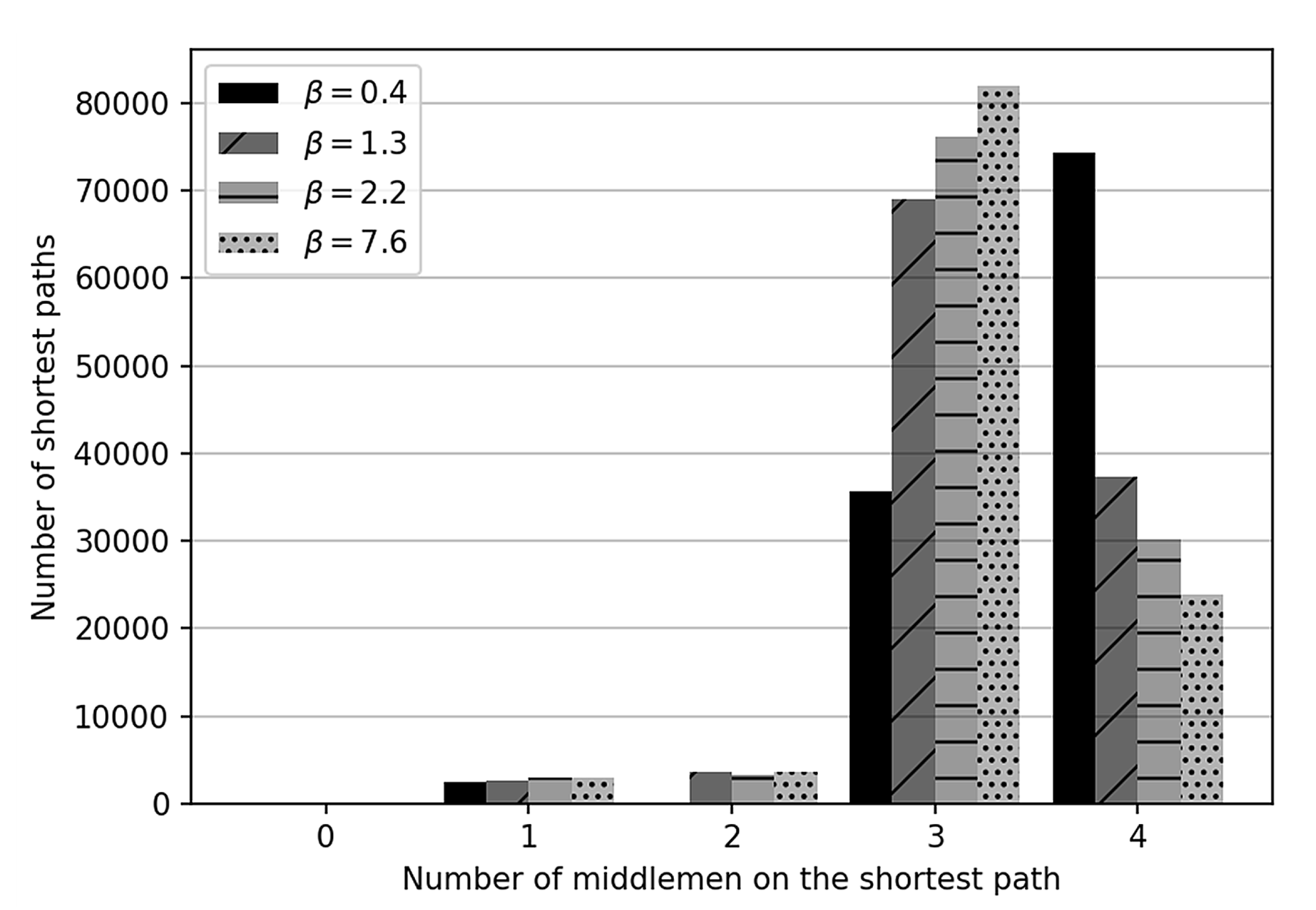
where $\alpha$ and $\beta$ are the business peering cost and the middleman price introduced in Section 2, respectively; $d_{(i,j)}\left(G\left(s\right)\right)$ denotes the number of middlemen on the shortest-path between providers i and j in the business graph G; $M_{i,j}$ depicts the extent of services bought by i from j through whatever path of middlemen providers this business is realized; and ${\mathcal{I}}_{i\in p_{j,k}}\left(G\left(s\right)\right)$ indicates whether i is on path $p_{j,k}$, i.e., the shortest path between j and k. If no path exists between i and j, then $d_{(i,j)}\left(G\left(s\right)\right)=\infty$. Therefore, the first term of the cost formula stands for the business link creation, the second term reflects the price to pay middlemen for reaching providers indirectly, and the third term is the income that is generated by acting as middlemen for other providers’ businesses.

As in [17], this game model reflects a setting in which building connections is expensive; however, an extensive direct network might be beneficial to build in order to limit the brokers to pay off. Likewise, the more connections a provider has, the more probable it will earn as a middleman, subsequently lowering the total cost. Naturally, providers try to limit their costs characterized in Equation (1). If the expense of an extra business link $\alpha$, the mediator cost $\beta$, and the business demand M are all fixed, the game comes down to the question of which new connections are worth being made so as to reduce expenses.

2.4. The Effects of Link Creation

For different sorts of equilibrium, stability conditions, lower and upper limits on the price of anarchy in network formation games, we refer the reader to [16,17,18]. Note that our model is different from the models found in the related work. The game variant that is the most similar to ours was introduced in [19]; however, contrary to that model where a player’s transit traffic brings about expense, in our arrangement, the more shortest paths that traverse a node, the more income is created to that respective player. For their arrangement, the authors of [19] demonstrated that the steady result of the game is consistently a tree, as more transit paths and the edge creation are not worth making lower distances to different nodes, once the graph is connected. In our game, the final graph $G\left(s\right)$ can also be a tree for high connection creation cost $\alpha$: both lower distance to different nodes, and mediating more business paths decrease the expense, hence, if edge creation is generally low cost, it is useful to make a few.

As portrayed in Section 2, we expect an underlying layered topology of providers. The objective of the work introduced in this section is to give an adequate condition under which there are no new connections made by the players. In case this condition is fulfilled, the underlying layered structure is along the stable state of our game, i.e., an equilibrium.

Assumption 1.

There are business links between providers originally, and these links organize nodes in a tiered topology, denoted by $G^0$, such as the one depicted in Figure 1a.

Let us number the tiers from top to bottom, $1,2,\cdots ,t$, and let $t^i$ indicate the tier that provider i belongs to. Let $C_i$ denote the set of providers that can be reached downwards in the tiered topology through provider i, i.e., $C_i=\{k\mid i\in p_{j,k}\forall j\mid t^j=1,t^k>t^i\}$, preferring peering links in Tier-1 to peering links in lower tiers. Now, we deduce the parametric cost saving when a new link is created.

Lemma 1.

If Assumption 1 holds, the highest cost reduction a new link between two nodes, i and j, can result in is

$$2\beta (t^i+t^j-2)|C_i||C_j|max(M_{kl|k\in C_i,l\in C_j},M_{kl|l\in C_i,k\in C_j})-2\alpha$$

(2)

Proof. 

Providers i and j, belonging to tiers $t^i$ and $t^j$ respectively, would both make a cost reduction for their children in $C_i$ and $C_j$ by interconnecting themselves with a new link and thus lowering the second term of Equation (1) of the children. At most, $t^i-1+t^j-1$ middlemen in upper tiers are shortcut from cross paths between the two sets of children with the new link. This number might be lower if any peering links exist between parents of i and j, or if they have the same Tier-1 parent. Note that we assume full mesh among Tier-1 providers in $G^0$. The cost allocated to middlemen is proportional with the extent of the business which is upper bounded by $max(M_{kl|k\in C_i,l\in C_j},M_{kl|l\in C_i,k\in C_j})$. The number of business relationships is given by $|C_i\left|\right|C_j|$, hence the result starting from the following formula:

$$\sum _{k\in C_i}\sum _{l\in C_j}\beta (t^i-1+t^j-1)(M_{kl}+M_{lk})-2\alpha .$$

□

Hindered by the complexity in a general tiered topology setting, we make the following assumption on the number of children each node has, and of businesses leaf nodes make.

Assumption 2.

$G^0$ contains a number of Tier-1 nodes connected in full mesh, and a tree subgraph under each Tier-1 node in which intermediary nodes have at least k children, and all leaf nodes are at the same depth t. Furthermore, any pair of leaf nodes exchange m amount of business; intermediary nodes do not act as service sellers or buyers.

Given the specific tiered topology of Assumption 2, we prove that the highest cost saving can be attained with new peering links in the topmost tier.

Lemma 2.

Under Assumption 2, the higher tier the nodes belong to, the larger the cost saving that is attained if they create a new link.

Proof. 

Under Assumption 2, the size of $C_i$ and $C_j$ are lower bounded by the number of leaves of perfect k-ary trees: $|C_i|\ge k^{t-t_i}$. The cost saving of two nodes i and j by creating a link is $2\beta (t^i+t^j-2)k^{2t-t^i-t^j}m-2\alpha$, where m represents the amount of business any pair of leaf nodes exchange under Assumption 2. By expressing $x=t^i+t^j$, it is easy to see that this cost saving is higher when $\frac{x-2}{k^x}$ is larger. As $k\ge 2$ and $x\ge 3$, the maximum is attained if $x=3$, i.e., $t^i=1$ and $t^j=2$, or $x=4$, i.e., $t^i=2$ and $t^j=2$. □

2.5. Sufficient Condition for Status Quo

We suppose that providers may turn to dynamic pricing schemes for middleman fees in order to bar the monetary incentives of new business link creation: as mentioned above, we seek the stable level of middleman prices when the status quo is kept, i.e., top tier providers demotivating low tier providers of making new business peerings. We determine this exclusionary price level in the assumed topologies.

Theorem 1.

Under Assumption 2, if all providers keep their price below $\frac{\alpha }{k^{2t-3}m}$, then topology $G^0$ is an equilibrium.

Proof. 

It is easy to see that the topmost tiers lose business if peerings are created underneath them. In such a topology $G^0$ that satisfies Assumption 2, the maximal middleman price $\beta$ for which no new links are worth being created between any two providers is given by $2\beta (t^i+t^j-2)k^{2t-t^i-t^j}m-2\alpha \le 0$ from which the upper bound on $\beta$ is $\alpha \frac{k^x}{(x-2)k^{2t}m}$ with $x=t^i+t^j$, according to Lemma 2. A statement is given by $x=3$. □

As a result of Theorem 1, the high tier providers have a motivating force to keep their broker costs low. The way that they need to save the status quo in terms of business relations among providers has a general constructive outcome on the whole system: the middleman cost of building up multi-provider businesses is upper limited. This bound is directed by the topology and the link creation cost.

2.6. The Stackelberg Game of Bertrand Competitions

Finally, in this section, we describe the equilibrium point of the network formation game with the assumption of initially non-existent peering relations between low tier providers, and of missing transit links between tiers.

Assumption 3.

Let us assume a 3-tier topology of providers, initially with no transit/peering links other than the Tier-1 full mesh. Furthermore, we assume that one transit link can be built by each Tier-2 (to a Tier-1) and Tier-3 (to a Tier-2) provider for no cost.

Bertrand competitions [26] describe interactions among suppliers that set prices and their customers that choose quantities to purchase from them at the prices set. The Bertrand competition model assumes that (i) there are at least two suppliers producing a homogeneous (undifferentiated) product and cannot cooperate in any way, (ii) suppliers compete by setting prices simultaneously and consumers want to buy everything from a supplier with a lower price (since the product is homogeneous and there are no consumer search costs), (iii) if suppliers charge the same price, consumers’ demand is split evenly between them, (iv) all suppliers have the same constant unit cost of the product or service, so that marginal and average costs are the same, and (v) each supplier has sufficient capacity to serve all customers.

Bertrand proved that, if suppliers chose prices strategically, then the competitive outcome would occur with the equilibrium price equal to marginal cost. In our specific case, the product to sell is the middleman service; therefore, we suppose that there is no maximum capacity imposed on the suppliers, and they all offer the same service.

We argue therefore that the game of setting individual middlemen prices in Tier-1 and Tier-2 are Bertrand competitions, as lower tier providers seek to build their transit link to one with the lowest price. Consequently, the Nash Equilibrium of the Bertrand game in Tier-1 results in a homogeneous ${\beta }_1^{*}$ middlemen price for all Tier-1 providers, covering the marginal cost of the full mesh linkage. Considering the average transit business they take care of, the following statement displays the value of ${\beta }_1^{*}$.

Lemma 3.

In equilibrium, Tier-1 providers all set their middlemen prices to ${\beta }_1^{*}=\frac{n_1(n_1-1)\alpha }{2\gamma m}$, where $n_1$ is the number of Tier-1 providers, γ is the fraction of businesses reaching Tier-1 and m is the grand sum of business matrix M.

Proof. 

As in a Bertrand duopoly competition, the only equilibrium price for the $n_1$ competing providers is at the marginal cost, since any provider setting a higher price would lose its customers. The total income is provided by the fraction of businesses flowing through Tier-1 providers, i.e., not via Tier-2 peering links, denoted by $\gamma m2{\beta }_1$. Supposing a uniform distribution of businesses flowing through the Tier-1 providers, and an equal share of peering costs, then applying ${\beta }_1^{*}$ covers the cost of full mesh peering at each Tier-1 provider. □

As Lemma 3 shows, the Bertrand game equilibrium is partly defined by the fraction of business ($\gamma m$) that will reach Tier-1 providers in the first place. This fraction is, in turn, dependent on the middlemen price that Tier-1 providers set, i.e., ${\beta }_1^{*}$ because, for certain Tier-2 providers that exchange relatively large amount of business, creating a direct link might be beneficial compared to paying the Tier-1 middlemen. In order to grasp this condition, we introduce the empirical distribution of such business amounts.

Definition 1.

Let us denote the empirical distribution of the amount of business between Tier-2 provider pairs by $f\left(\mu \right)$. Similarly, let us denote the distribution of those between Tier-3 providers by $g\left(\mu \right)$.

Both Tier-2 and Tier-3 providers have the option of creating peering links in case it is less costly than dealing with middlemen. As middlemen prices grow, more and more provider pairs decide so. Therefore, the fraction of business from Tier-2 to Tier-1, and from Tier-3 to Tier-2, decreases with the rise of middlemen prices: demand is monotone decreasing in ${\beta }_1$ and ${\beta }_2$, respectively. Furthermore, peering links are created in the decreasing order of the amount of business between the two endpoints, as the middlemen price grows. This phenomenon creates a Stackelberg game [21] nature of the middlemen price setup between Tier-1 (being the leaders) and Tier-2 (being the followers). The Stackelberg competition suits well the situation as the leaders, i.e., Tier-1 providers move first by setting their middleman prices homogeneously, and then the followers, i.e., Tier-2 providers move sequentially, deciding about the link creation in function of Tier-1 prices. Let us see how we can deduce the equilibrium price in Tier-2.

Lemma 4.

In equilibrium, the Tier-2 providers’ middlemen price is

$${\beta }_2^{*}=\frac{\alpha }{2\delta m}\left(n_1(n_1-1)+n_2(n_2-1){\int }_{\frac{2\gamma m}{n_1(n_1-1)}}^{\infty }f\left(\mu \right)d\mu \right),$$

where δ is the fraction of business reaching Tier-2, and $n_2$ denotes the number of Tier-2 providers.

Proof. 

Similarly to Lemma 3, in equilibrium, all Tier-2 providers apply the same middlemen price ${\beta }_2^{*}$, and their total income precisely covers their cost. The overall Tier-2 income is given by the Tier-3 providers, with their business not traversing through their own peerings, i.e., $\delta m2{\beta }_2$. The middlemen fee and the creation of peerings constitute the total cost of Tier-2 providers, i.e., $\gamma m2{\beta }_1^{*}$ and $2\alpha {\int }_{{\mu }_2^p}^{\infty }f\left(\mu \right)d\mu \frac{n_2(n_2-1)}{2}$, respectively, where ${\mu }_2^p$ denotes the amount of business over which the peering is cheaper than via Tier-1 middlemen. This latter condition gives ${\mu }_2^p=\frac{\alpha }{{\beta }_1^{*}}$. Substituting the value of ${\beta }_1^{*}$ with $\frac{n_1(n_1-1)\alpha }{2\gamma m}$ from Lemma 3 yields the formula for ${\beta }_2^{*}$. □

Finally, we can draw the amount of business that Tier-3 providers will carry through Tier-2 providers. The following statement expresses the necessary formulas for substituting $\delta$ and $\gamma$ in Lemmas 3 and 4.

Lemma 5.

In equilibrium, the fraction of business flowing through Tier-2 and Tier-1, respectively, are: $\delta m={\int }_0^{\frac{\alpha }{{\beta }_2^{*}}}\mu g\left(\mu \right)d\mu$, and $\gamma m={\int }_0^{\frac{\alpha }{{\beta }_1^{*}}}\mu f\left(\mu \right)d\mu$.

Proof. 

Similarly to the proof of Lemma 4, let us denote by ${\mu }_3^p$ the amount of business over which the peering is cheaper than through Tier-2 middlemen. Analogously to ${\mu }_2^p$, ${\mu }_3^p=\frac{\alpha }{{\beta }_2^{*}}$. The statement then follows. □

The equilibrium prices can be determined numerically if $n_1,n_2,f\left(\mu \right),g\left(\mu \right),m,\alpha$ are given. Moreover, if Tier-3 providers select their Tier-2 transit partner randomly, and the ratio between the number of Tier-2 and Tier-3 providers is sufficiently small, the central limit theorem might be applicable in order to determine $f\left(\mu \right)$ based on $g\left(\mu \right)$. Hindered by the analytic complexity of the problem, we now turn to a comprehensive numerical analysis of the business network formation game.

3. Numerical Analysis

This section first describes what simulation settings we used to validate our theoretical results. After the description of simulation setups in the first part, we show the results of the simulations in the second part.

3.1. Iterative and Two-Phase Simulations

In order to perform further analysis on our theoretical results, we constructed two simulation environments, an iterative and a two-phase approach. We implemented both versions of the simulator on Linux in Python (2.7) [27] as it is an ideal language for prototyping. Since our data model is based on graphs, we used the NetworkX [28] Python library to represent the model and to handle graph operations efficiently.

3.1.1. The Iterative Simulation Setting

As we look at the advancement of the business arrangements that characterize the present Web, we suppose its current topology as the underlying state of our simulations: we used the topology presented in Section 2. We made three levels, plus an extra layer of SAPs underneath Level 3. In order to satisfy the prerequisite on the minimum width applied in Section 2.4, we picked an arbitrary number of children for every node in the tree from a uniform distribution between 5 and 10. Consequently, the simulations comprised of roughly 300 nodes.

We assume that the business agreements are being set up between Level 3 providers since they might want to make resource slices interconnecting their SAPs. We made the case of heterogeneous business interests between all SAP–SAP pairs, e.g., making the case of local busy areas that clients from different customer facing providers are bound to pick for accessing services in resource slices. We built the business matrix M by utilizing Gaussian distributions that top at arbitrarily chosen providers.

The connection creation and middleman costs, $\alpha$ and $\beta$ as introduced in Section 2, are the parameters of interest that can be investigated comparative with one another. We chose to fix the value of $\alpha$ to 1 and performed simulations with a few $\beta$ values relative to it.

The iterative simulations are partitioned into rounds with each containing an evaluation: all providers attempt to decide their ideal arrangement of business associations. In the event that there are no further changes from one round to the next, the simulation is considered to be in a stable state, and this final state is an equilibrium topology of the game.

Inside a round, providers check for every other provider if another link is worth building up dependent on the cost characterized in Section 2. In the event that the chosen fellow provider likewise chooses to make the business connection, the corresponding edge will be added to the graph. Existing business associations are additionally analyzed in every round whether their upkeep is still beneficial to the two players or not—disadvantageous links are dropped. In each iteration, we check if a business relation is worth being established between all provider pairs which gives us a $n^2$ computational complexity for each round. In the complexity of the whole simulation, $n^2$ is multiplied with the number of iteration rounds until the equilibrium is reached.

In Figure 2, we illustrate the distribution of business path lengths in the graph: the figure shows the quantity of agents along the briefest business paths in the steady graphs resulted for various values of $\beta$. The greatest number this metric can reach is 4, as, for this situation, there are no alternate routes in the tree: the shortest path is through Tier 1 providers. One can understand how courses abbreviate as $\beta$ grows, while most associations are framed between upper-level providers, subsequently numerous 3-hop and 4-hop paths appear. The quantity of paths with 0 mediators is near 0 in all situations, checking that peerings are rarely created between Tier 3 providers, as concluded in Figure 3.

To further improve the flexibility of our simulation environment, we made other system descriptor features configurable. While we achieved adapting the environment to reality to a greater extent, these extensions also introduced an instability in the simulations. Thus, we redesigned the simulation framework and defined another simulation approach, consisting of two phases, focusing on the analysis of opposing business forces defined in Section 1.

3.1.2. The Two-Phase Simulation Setup

In the advanced simulator, we have two separated phases: (i) the calculation of expenses after establishing all peering relations, (ii) increasing $\beta$ separately by tiers until reaching a threshold value of cross-business loss.

In the first phase, we establish all feasible peering connections, i.e., providers having sufficient business demand towards each other. The topology has three tiers and an additional layer of end users and service providers (represented by SAPs) as before. We have several setups with balanced and unbalanced tree-like topologies. In the simulation after connecting all nodes except the bottom ones with all feasible peerings, we calculate an expense value for each provider. This is based on the business demand matrix we generated and the usage of peering relations without considering income. Peering relations calculated as per connection while mediated services are weighted with the forwarded demand. This value represents a stable value a provider is able to achieve in one of the extreme positions.

The second phase uses the very same topology structure defined in step (i) without any peering relations. Then, starting with Tier-1 providers, all nodes increase their $\beta$ value with a predefined increment. They continue this behavior until a given percentage of their through-business is lost. A provider can lose business if a parent provider (in the tree structure) reaches its own expense value calculated in phase (i). After every $\beta$ rising step, we calculate the expense of each provider based on the current market environment of middlemen prices. If the recently calculated expense value is higher than the value calculated in (i), the provider removes its businesses from the system: these $\beta$ values are no longer beneficial. Thus, the respective business is removed from all parent nodes in the tree topology, increasing their loss. A provider stops raising its middleman price as soon as it loses a considerable amount of business. When all providers in Tier-1 fix their $\beta$ values, we start the procedure again with the Tier-2 providers, and so on. Simulation is concluded if each and every provider has stabilized its $\beta$ value.

This simulation version has a decreasing complexity in each round as more and more providers freeze their business connections and drop out of the set of potential link creators. In the worst case, however, if all providers stop at the same time, then $n^2$ is the computational complexity. The number of simulation rounds depends on the resolution by which the providers raise their $\beta$ values. On the other hand, they stop based on their expenses, i.e., the number of iterations is resulted from the ratio of the expense value of the providers and the $\beta$ increment. Compared to this complexity, the authors of [19] prove that their network formation model converges in $O\left(n^5\right)$.

Topology structure of the two-phase simulation consists of four Tier-1 providers and four children below each and every node in the tree, forming four tier levels overall. Similar to the iterative simulation, we have about 300 network providers in the simulation.

In the two-phase simulation, we differentiated balanced and unbalanced topology structures as they can diverge in their behavior as seen in case of the iterative simulations. In case of a balanced structure of providers, we assume that all nodes have the same number of consumer (child) providers; this number was four in the simulations presented here. In an unbalanced topology, however, we allow providers to have children from the range of 1 and 5, inclusive. This approach introduces an additional factor of instability in the simulations.

In these simulations, we fixed the value of $\beta =1$, and, with both balanced and unbalanced cases, we run simulations with $\alpha$ being 1, 10, 50, relative to $\beta$.

3.2. Simulation Results

In the following, we introduce the results of the two simulation setups. First, we detail the measurements of our iterative simulation method, then that of the two-phase model. These kinds of simulations are usually sensitive to the selected initial parameter values. Therefore, we made several measurements for each $\beta$ value with random initial setup and the presented results show the aggregated measurements of those.

3.2.1. Iterative Simulation Results

We run hundreds of simulations, assuming several different initial setups. Here, we compare the stable topologies from the perspective of various metrics.

In Figure 3, one can see how the adjustments in the middleman cost, i.e., $\beta$’s worth, change the structure of the layered graph. The figure shows the quantity of new links, isolated by tiers, created at different middleman prices, appeared on a logarithmic x-axis. When the middleman price is sufficiently low, i.e., left extreme, the foundation of new business peerings is rare, even non-existent. As $\beta$ is increased contrasted with the upkeep cost of a business connection, i.e., $\alpha$, each provider begins to abbreviate their business paths in order to stay away from costly mediators in upper tiers. As the two players must consent to shape a business peering and the traffic request between Tier 3 providers is only once in a while large enough at both ends, most business associations include at least one upper-level provider. At the same time, the rest of the transit business accumulated towards the top-tier providers decrease, thus a portion of the settled business connections of Tier 1 providers are dropped in the later rounds. Roughly $\beta =4.3$ is where providers course most business through peerings.

Instinctively, the more mainstream a Tier 3 provider’s territory is, the shorter the paths others might want to arrive at it through. In view of Figure 3, we picked four intriguing cases: (i) $\beta =0.4$ with the predetermined number of business peerings in all levels, (ii) $\beta =1.3$ resulting in that the number of associations of Tier 1 providers is around its pinnacle, (iii) $\beta =2.2$ making Tier 1 providers drop a few associations while business peering is on the ascent in Tier 3 and (iv) $\beta =7.6$ with which a stable combination in the quantity of new business associations has been reached.

Figure 4 shows the aggregate sum of services sold by the providers, which equals the column sum of the respective provider in the business matrix, partitioned into four segments. On the y-axis, we depict the average length of the paths that leads to the providers that belong to the specific range. For each of the four $\beta$ values, a diminishing pattern can be seen on all sub-figures. Furthermore, across the sub-figures, a general dropping trend of lengths is additionally detectable as $\beta$ is growing, making the foundation of new business associations more valuable.

3.2.2. Two-Phase Simulation Results

In the previous case, we showed how changing the middleman cost affects the number of newly introduced business connections in the volatile simulation environment. As an extension, here we demonstrate the direct effects different $\alpha$ values have on $\beta$. Furthermore, in this more stable setup, we explore how topological changes influence the ratio of their values in equilibrium.

We can follow how $\beta$ values in various tier levels changed during the simulation in Figure 5. We show simulation results with three setup parameters: the difference is in the price of a peering relationship, i.e., $\alpha$.

We see that the structure of middlemen prices is mostly independent from the change of the ratio of $\alpha$ and $\beta$ as Tier-1 providers always have the lowest middlemen price, and this value is growing towards the leaves. However, the overall middlemen price depends on the predefined cost of a peering. If it is more expensive to maintain peering relations, transit providers can raise their overall $\beta$ values.

Comparing the balanced topology to a more diversified structure, results, depicted in Figure 6, suggest a difference in $\beta$ distribution. The bottom tier providers do not reach the highest middlemen price, but Tier-2 providers do. In such an unbalanced topology setup, Tier-3 providers with a small number of parents fall out of the simulation early as they reach the threshold on business loss even after a small change. A larger set of node batches stay in the simulation allowing the intermediate providers to raise their middleman prices. Even if some of their customers fall out, it is only a small percentage of the total demand. This phenomenon allows Tier-2 providers to raise their $\beta$ values to a point where Tier-3 providers only have a small margin for their own $\beta$ price increment.

Finally, Figure 7 shows that, despite the difference in $\beta$ values of the tier levels, their payoff is relatively close to each other. As business is aggregated upwards in the topology, the difference in the amount of transited business accounts for this observation. Network and compute resource providers closer to the root of the tree aggregate more cross-businesses taxing with relatively low middleman prices, while bottom tier providers deal with a small amount of business, but higher unit prices.

4. Discussion

The objective of our business case investigation was to characterize conceivable business structures for multi-provider cloud-based service offerings. Assuming the current multi-tier ISP structure for worldwide connectivity services as a starting point, we began our examination by investigating why and how the current ISP structure may change into new business connections. Beginning from the layered ISP order, we described a network formation game in which players represented the ISPs; link creation represented business associations with an upkeep cost; operational expenses and incomes were determined to be dependent on paid and received middleman costs offering mediator services. Our work was inspired by the body of related work addressing the phenomenon of growing number of peering relations between ISPs. In contrast to those work, our study focuses on agreements between 5G and cloud infrastructure providers, either directly or via mediating parties, instead of exchanging Internet traffic through either peering or transit relations studied in the related research papers. In our work, network traffic related to the cloud services was assumed to be directed along the conventional ISP structures individually, since new business connections do not suggest physical proximity of the respective providers.

We built a cost function model, partly resembling to those found in the research domain of network formation games that characterized all the important aspects of the participating providers. With a few suppositions (see Section 2.4) on the initial connection topology among the providers, we determined an upper bound condition on the middleman price as an element of peering expenses and topology traits, i.e., if ISPs might want to save the current status quo concerning their transit links, at that point, they need to keep their middleman fees low. The systematic outcomes’ reliance on the topology guaranteed distinctive prices for every tier.

In our simulations, we recreated games with various middleman prices for different starting ISP graphs. In a 3-tier topology, our outcomes uncovered that with expanding middleman prices the quantity of new business associations ascended until a stable state where no new peerings were reasonable. Results likewise demonstrated that mutual consent for peering among the lower Tier 3 providers seldom happened; instead, the Tier 2 providers drew in a large portion of the new businesses because of their capacity of collecting the transit requests from the sub-ordinate ISP levels.

5. Conclusions

Cloud computing has grown to be the de facto standard to host online services by offering less expensive and simpler answers for resource and application management. Distributed infrastructure, e.g., edge and fog computing, is by all accounts the following significant advance forward to boost service offerings in a cost-productive way. As virtualized services can adapt to the rapidly changing manner of customer demands, negotiation on service chain establishment should follow this approach. The current status of fragmented ownership of distributed compute and network resources, nonetheless, will make it vital for Telco actors to coordinate (and to contend) in their disseminated cloud-based offerings. What sort of business relations will develop among Telcos is an open question.

In our research, we evaluated how this transformation can influence network structure and which factors can motivate service providers in adjusting their mediation price on virtual services. In Section 2, we have formalized our approach as a network formation game and derived analytical results on the equilibrium conditions of it. In Section 3, we carried out numerical simulations on various initial ISP topologies and, consolidating our predication based on statistical analysis, we argued that business peering based on mutual desire are mostly beneficial for higher tier actors of the network.

In our future work, we plan to introduce a new possible action for the network providers to avoid monopolistic transit price settings. If several transit providers were present in a physical neighborhood in a realistic scenario, lower level (Tier-3) providers would be able to attach to another transit provider instead of their current one, inducing a newly introduced predefined home update cost, but making the competition fiercer.