Abstract
Premature ventricular contraction (PVC) is a common cardiac arrhythmia that can occur in ordinary healthy people and various heart disease patients. Clinically, cardiologists usually use a long-term electrocardiogram (ECG) as a medium to detect PVC. However, it is time-consuming and labor-intensive for cardiologists to analyze the long-term ECG accurately. To this end, this paper suggests a simple but effective approach to search for PVC from the long-term ECG. The recommended method first extracts each heartbeat from the long-term ECG by applying a fixed time window. Subsequently, the model based on the one-dimensional convolutional neural network (CNN) tags these heartbeats without any preprocessing, such as denoise. Unlike previous PVC detection methods that use hand-crafted features, the proposed plan rationally and automatically extracts features and identify PVC with supervised learning. The proposed PVC detection algorithm acquires 99.64% accuracy, 96.97% sensitivity, and 99.84% specificity for the MIT-BIH arrhythmia database. Besides, when the number of samples in the training set is 3.3 times that of the test set, the proposed method does not misjudge any heartbeat from the test set. The simulation results show that it is reliable to use one-dimensional CNN for PVC recognition. More importantly, the overall system does not rely on complex and cumbersome preprocessing.
1. Introduction
The heart is a vital organ of the human body and has four chambers: right atrium, right ventricle, left atrium, left ventricle. These four chambers cooperate in providing power for blood flow in the blood vessel. First, the oxygen-poor blood flows through the right atrium and right ventricle in turn, and finally reaches the lungs. Then the oxygen-poor blood absorbs oxygen from the air in the alveoli. With the left atrium and left ventricle’s work, the rest organ and tissue will receive the oxygenated blood. The most intuitive feeling of this process is the heartbeat. Every heartbeat moves blood forward through the arteries. Heart rhythm, which is the heartbeat pattern, is a critical clinical indicator to assess whether the heart is working correctly. Healthy heart rhythm is orderly and uniform. Abnormal heart rhythm, also called arrhythmia, is usually closely related to cardiovascular disease (CVD). According to the World Health Organization (WHO), CVD is widespread globally. Taking America and China as examples, ten people die every 6 min in America from CVD, and nearly 20.7% of China residents suffer from CVD [1].
Although there are many origins of the arrhythmia, premature ventricular contraction (PVC) caused by an ectopic cardiac pacemaker located in the ventricle is the most common cause. Moreover, PVC is also related to multiple conditions, such as myocardial infarction (MI), left ventricular dysfunction (LVD) [2,3]. Electrocardiogram (ECG), which can record the heart’s electrical signals, is a non-invasive and effective visualization tool widely used by cardiologists [4]. A normal heartbeat generates four entities with different shapes in ECG—a P wave, a QRS complex, a T wave, and a U wave, as shown in Figure 1.
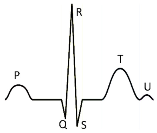
Figure 1.
There is a normal heartbeat in electrocardiogram (ECG). The atria’s depolarization caused the P wave; the ventricles’ depolarization caused the QRS complex; the repolarization of the ventricles caused the T wave; the repolarization of the Purkinje fibers caused the U wave.
It is worth mentioning that the long-term ECG is more clinically significant for the diagnosis of PVC. However, it is time-consuming and arduous for cardiologists to analyze many long-term ECGs. Therefore, accurate and automatic searching for PVC from the long-term ECG is crucial for improving cardiology workflow efficiency.
In recent years, many researchers have developed various algorithms to search for PVC from ECG, as summarized in Table 1. Most of the algorithms manually extract morphological-based features. Manikandan et al. designed a set of temporal characteristics and proposed a decision-rule-based detection algorithm. The suggested method achieved an average sensitivity of 89.69% and specificity of 99.63% based on the MIT-BIH arrhythmia database [5]. Jun et al. extracted six features from the ECG signal and developed a classification algorithm on TensorFlow [6], an open-source machine learning platform. This algorithm used an optimized deep neural network (DNN) whose input is the six features, as the classifier. These six characteristics are R-peak amplitude, R-R interval time, QRS duration time, ventricular activation time, Q-peak, and S-peak amplitude. The experimental results based on the MIT-BIH arrhythmia database achieved 99.41% accuracy [7].

Table 1.
Various algorithms for detecting premature ventricular contraction (PVC) in recent years.
Hadia et al. not only summarized a feature extraction procedure based on the Principal Component Analysis (PCA) and waveform estimation but also combined the extracted features and k-nearest neighbor (KNN) algorithm. The classification sensitivity of this model is 93.45% [8]. Atanasoski et al. presented an unsupervised clustering method based on the R-R intervals and morphological rule. This algorithm does not rely on pre-existing labels and has an excellent overall accuracy above 99.5% and specificity above 99.6% [9]. Junior et al. developed a system based on threshold adaptive algorithm and wavelet transform for PVC detection. The result validated on the MIT-BIH arrhythmia database reported that Daubechies 2 wavelet mother is more indicated compared with Coiflets and Symlets [10]. Oliveira et al. proposed a simplified set of features extracted from geometric figures constructed over QRS complexes and selected the most suitable classifiers based on the analytic hierarchy process (AHP). The results of this method indicated that the artificial immune system (AIS) classifier with the geometrical features is the best suggestion for PVC recognition [11].
Considering that labeled ECG data is rare and precious, Lynggaarda suggested a multivariate statistical classifier that used robust designed features and a regularization mechanism. Even though this classifier’s input is a very sparse amount of expert annotated ECG data, this model’s average accuracy, specificity, and sensitivity are above 96% by using the MIT-BIH arrhythmia database [12]. Sokolova et al. recommended a set of weighted shape parameters from the different QRS shape metrics and designed a two-stage PVC detection rule. All these shape parameters are in the time and frequency domains. It is worth noting that this method achieved good results on the multi-lead ECG database: the St. Petersburg INCART 12-lead Arrhythmia Database [13]. Rizal and Wijayanto proposed a simple and low computation method. This method only used six characteristics obtained by the multi-order Rényi entropy and chose the support vector machine (SVM) with six kernels to detect PVC. The simulation results obtained 95.8% accuracy [14]. Chen et al. designed an algorithm to distinguish the QRS complex’s peak points and proposed a PVC identification system based on the back-propagation neural network (BPNN). The system’s input is a set of features obtained from the QRS complex peak points. The simulation result’s average accuracy attains 97.46% on the China Physiological Signal Challenge 2018 (CPSC2018) Database [15].
Mazidi et al. evaluated three sets of ECG features and two classifiers on the field programable gate arrays (FPGAs). These three groups of characteristics come from time-domain based on the reconfiguration Pan–Tompkins algorithm, frequency-domain based on the Haar wavelet algorithm, and time-domain combination of frequency-domain based on the above two. The two classifiers are the SVM and the Naive Bayes [16]. Besides, Mazidi et al. introduced six robust features extracted by morphological assessment, polynomial curve fitting, discrete wavelet transform, and nonlinear analysis. Moreover, this literature used an SVM with a linear kernel to recognize PVC. This algorithm acquires the overall accuracy of 99.78%, with a sensitivity of 99.91% and 99.37% specificity for the MIT-BIH arrhythmia database [17]. Allami applied an artificial neural network (ANN) to classify the features extracted through morphological and statistical methods. The proposed method resulted in a sensitivity and accuracy of 98.7% and 98.6%, respectively, on the MIT-BIH arrhythmia database. Additionally, this method is computationally simple and suitable for real-time patient monitoring. [18]. Chen et al. extracted three features and provided these to a classifier based on the perceptron model. The three characteristics are the ratio of the QRS areas, the previous R-R interval, and the last R-R interval ratio to the next RR-interval. The experiments applied to the MIT-BIH arrhythmia database achieved high accuracy with a sensitivity of 98.7%. Moreover, this method’s logic resources and power consumption are low, so it is suited for wearable monitoring [19]. Jeon et al. designed a model based on the error backpropagation algorithm and used four characteristics to detect PVC. These features are R-R interval, Q-S interval, Q-R amplitude, and R-S amplitude. The proposed approach’s overall accuracy was above 90%, with testing on the MIT-BIH arrhythmia database [20].
With the popularity of deep learning and outstanding performance in other fields, researchers use deep learning to monitor PVC. Many experts used deep learning to detect PVC. Zhou et al. developed a reliable ECG analysis program to detect PVC. This system consists of two parts: data preprocessing and a recurrent neural network (RNN) with long short-term memory (LSTM). The accuracy of this method based on the MIT-BIH arrhythmia database is 96–99% since the RNN is good at processing time-series signals [21]. Zhao et al. combined the Modified Frequency Slice Wavelet Transform (MFSWT) and CNN, which has 25 layers, to search for PVC from 12-lead ECG data provided by the CPSC2018 Database. The MFSWT can transform one-dimensional time-series signals into two-dimensional time-frequency images as the input of the CNN. The test results of this method achieved a high accuracy of 97.89% [22].
Li et al. used three types of wavelets to convert single-channel ECG signals to wavelet power spectrums and constructed a CNN consisting of three convolutional layers, two max-pooling layers, and a rectified linear unit layer, a fully connected layer. These three wavelets are Morlet wavelet, Paul wavelet, and Gaussian derivative. The CNN receives and processes the transformed wavelet power spectrums, then labels it. It is commendable that the generalization ability of this method is excellent. The validation results on the American Heart Association (AHA) database achieved an overall F1 score of 84.96% and an accuracy of 97.36% with the training data from the MIT-BIH arrhythmia database [23]. Gordon and Williams developed a PVC detection algorithm based on autoencoder and random forest classifier. The proposed autoencoder consists of two parts. The first part is an encoder with two convolutional layers used for encoding the ECG to a latent space representation, which is low-dimensional and effective. The second part is a decoder with transposed convolutional layers for decoding the latent space representation to recover the ECG. The random forest classifier composed of 10 decision trees takes the latent space representation as input and annotate it. This algorithm achieved an overall accuracy above 97% on the MIT-BIH arrhythmia database [24]. Rahhal et al. report a model based on the Stacked Denoising Autoencoders (SDAs) networks and DNN to search PVC from the multi-lead ECG signals. The SDAs networks have the function of extracting features. The DNN classifies the ECG according to the obtained features. In the experiments with St. Petersburg INCART 12-lead Arrhythmia Database, the results are 98.6% and 91.4% respectively for accuracy and sensitivity [25]. Hoang et al. proposed a PVC detection algorithm for the multi-leads ECG and deployed it on wearable devices. The algorithm includes the Wavelet fusion method, Tucker-decomposition, and CNN, which has six layers: two convolutional layers, two max-pooling layers, a fully connected layer, and a dropout layer. Although this algorithm’s accuracy is 90.84% on the 12 lead ECG St. Petersburg Arrhythmias Database, the proposed method is scalable to analyze 3-Lead to 16-Lead ECG systems [26]. Liu et al. applied deep learning to develop models that can search PVC from children’s ECG. The children’s ECG used in the experiment are JPEG images from the hospital. This study’s experimental results show that the Inception-V3 with waveform images and one-dimensional CNN with time-series data extracted from waveform images can detect PVC in children [27].
According to Table 1, various algorithms for detecting PVC in recent years, we can quickly obtain the following conclusions. First, the amount of morphological-based literature is more than Deep Learning. Secondly, relevant researchers prefer these three classifiers: DNN, SVM, and Pattern matching. Third, the R-R interval is recognized by most research as a useful feature, but the other features do not seem to be unanimously recognized by most research. Finally, the model’s performance based on morphology is slightly better than that of Deep Learning, thanks to the expertise of the person who designed the feature.
Although the morphological-based methods have achieved good results, they still have some limitations. First of all, these methods rely heavily on professional knowledge about ECG and signal processing to design the rules for extracting features. Second, these features extracted manually are biased and varies from person to person. Finally, most morphological-based methods are also limited by each wave’s positioning algorithm in a heartbeat. For example, the inaccurate positioning of Q wave and S wave will directly affect the performance of detecting PVC, in literature 20.
Fortunately, some methods based on deep learning mostly avoid these limitations. The approach based on deep learning has the following three characteristics: first, it can automatically extract features, such as by convolution kernels; second, it can continuously optimize and select features during the training process to make the features non-redundant, such as by max-pooling; third, it can directly analyze the preprocessed heartbeats.
However, these existing methods based on the Deep Learning require preprocessing of the original ECG or the cooperation of other classifiers. The method proposed in the literature [21] has many preprocessing steps, such as resampling, denoising, signature detection, normalize. The studies [22,23,26] performed wavelet transform on the ECG to obtain 2-D time-frequency images. Moreover, the research [24,25] used the features extracted by a trained autoencoder to recognize PVC. There is no doubt that the above methods are computationally intensive.
Furthermore, identifying PVC is very complicated because the PVC waveform is quite uncertain, even for the same patient. Figure 2 shows some PVC waveforms from the same person. Therefore, achieving a real-time classifier with high accuracy and sensitivity is a challenging problem to address.
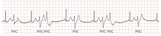
Figure 2.
There are some PVC waveforms from the same person. The waveforms of these PVCs in the picture are different, especially the second and third.
In summary, considering the limitations of manually extracted features and the advantage that deep learning can automatically extract features, this study proposed a method based on one-dimensional CNN. This method can autonomously learn features from the labeled ECG data with supervised learning to avoid the manually extracted features’ bias. Secondly, this method does not rely on professional knowledge that is used to design features. Third, this method does not have to preprocessing steps such as denoising and can directly process and analyze heartbeats, which will improve the efficiency of searching for PVC from ECG. Notably, the MIT-BIH arrhythmia database [28,29] will assess the validity of our proposed method. The following is the arrangement of the remainder: Section 2 describes the dataset, proposed framework, and evaluation measures; Section 3 presents and discusses the results; finally, Section 4 gives the conclusion and directions.
2. Materials and Methods
2.1. Materials
The MIT-BIH arrhythmia database is the first generally available benchmark database for the evaluation of arrhythmia detectors. The database contains 48 long-term Holter recordings obtained from 25 men subjects and 22 women subjects. Each of the 48 records numbered from 100 to 234 inclusive with some numbers missing, is slightly over half an hour-long and has two leads (the upper signal and lower signal). The upper signal in most records is a modified limb lead II (MLII), but the lower signal is occasionally V1, V2, V4, or V5. It is worth noting that recordings 201 and 202 came from the same male subject and the rest records are from a different subject. Furthermore, all records in this database are annotated by two or more cardiologists independently. Detailed annotations and a large number of records have made most researchers admire this database.
To effectively use this database, the Association for the Advancement of Medical Instrumentation (AAMI) recommends that records 102, 104, 107, and 217 are discarded because of the pacemaker or presenting complete heart block. Besides, this study designed three schemes to divide the remaining ECG records for evaluating the proposed method’s effectiveness. Table 2. Splitting data into training and test sets. and Figure 3 showed the grouping schemes. It is worth mentioning that blind cross-validation cannot reasonably evaluate the performance of the model and comes with risks associated with label leakage.
Table 2.
Splitting data into training and test sets.
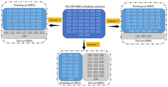
Figure 3.
Splitting data into training and test sets. The information in this figure is the same as in Table 2. Splitting data into training and test sets.
Taking Scheme 1 in Table 2, splitting data into training and test sets, and Figure 3, splitting data into training and test sets, the information in Figure 3 is the same as in Table 2. As an example: the “DS1” and “DS2” represent the training set and the test set. The “101” represents the records number in the MIT-BIH arrhythmia database. The “N” and “V” respectively represent the number of the regular beat and PVC in the dataset. The “Ratio” means the ratio of the samples’ number in the training set and the test set, such as (35640 + 2851)/(33868 + 2548) = 0.9778. Notably, most researchers adopt Scheme 1, which AAMI suggested and can also guarantee a reasonable comparison between our proposed method and other studies. Scheme 2 and Scheme 3 can evaluate the proposed method’s performance in the situation that the number of samples in the training set is higher than the test set.
2.2. Methodology
Figure 4 shows a block diagram of the proposed study, with a view showing the proposed method’s flow. Initially, this research divided each ECG signal from the modified limb lead II (MLII) into separate heartbeats according to a fixed time window and an R peak detection algorithm. The duration of each heartbeat composed of 433 sampling points is 1.2 s. Then the proposed model based on the one-dimensional CNN takes these heartbeats as input to search PVC.
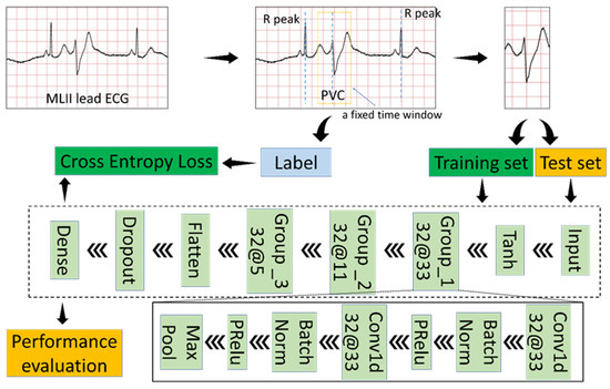
Figure 4.
Block diagram of the proposed study.
2.2.1. Generate Input Data
Since the MIT-BIH arrhythmia database provides detailed annotations, including R-peak locations and rhythms’ label, input data is the raw signal directly corresponding to each heartbeat without any preprocessing. We use a fixed-size window to extract the heartbeat from the MLII ECG lead since each heartbeat’s dimension must be the same as the proposed classification model’s input dimension. The window’s size is 433, and the window’s center is the location of R-peak. Because R-peak detection algorithms [30,31,32,33], such as Pan–Tompkins algorithm, can accurately find the R-peak point. We use the R-peak location in the database directly without developing a novel method to detect R-peak location.
2.2.2. Classifier Structure
First, the proposed model uses the Tanh function to transform the input data. The Tanh function can normalize the input data between –1 and 1, which is conducive to the training of the model. Equation (1) is the definition of the Tanh function.
Secondly, the proposed model has three convolutional groups, as shown in Figure 4. Each convolutional group contains five layers. A one-dimensional convolutional layer is a powerful tool that results in a feature map representing a detected feature’s positions and intensity in an input. Convolution is a simple operation:
(1) Flip the convolution kernel;
(2) Move the convolution kernel one data point at a time along the input vector;
(3) Calculate the dot product of two corresponding points at each position;
(4) The generated sequence is the convolution of the convolution kernel with the input vector.
For example, specifying the input vector and the convolution kernel are discrete sequences, then the definition of convolution is as follows.
The batch normalization layer allows the neural network to complete training faster and more stably by normalizing the feature map and does the following during training time [34]:
(1) Compute the mean and variance of the layer’s input;
(2) Normalize the layer’s input using the mean and variance;
(3) Obtain the output with scaling and shifting;
Notice that m is the number of samples per batch, ϵ is a small constant for numerical stability. Additionally, γ and β are learnable parameters.
The Parametric Rectified Linear Unit (PReLU) is an excellent activation function and has become the default activation function for many neural networks [35]. Although PReLU will introduce slope parameters, the increase in training costs is negligible. The mathematical definition of PReLU is as follows.
The max-pooling layer can reduce the computational cost and effectively cope with the over-fitting phenomenon by down-sampling and summarizing in the feature map. Additionally, the max-pooling layer provides fundamental translation invariance.
Take ‘Group_1 32@33’ in the Figure 4 block diagram of the proposed study as an example to comprehend the convolution group. ‘Group _1’ is the convolution group’s name; ‘32@33’ represents the number and size of the one-dimensional convolutional layer’s convolution kernels in the convolution group.
The proposed model also includes the Flatten layer, the Dropout layer, and the Dense layer. The Flatten layer collapses the spatial dimensions to make the multidimensional input one-dimensional. The Dropout layer refers to ignoring some neurons during a forward or backward pass to prevent over-fitting [34]. The Dense layer is a basic neural network layer and functions as a ‘classifier.’
Table 3 and Table 4 give the necessary parameters and the dimensional change of the proposed model’s input data. The random seed in this study is 0, which can ensure that the experimental results are reproducible. Dropout in Table 3 refers to the probability of an element to be zeroed.
Table 3.
Parameters of the proposed model.
Table 4.
The dimensional change of the input data in the proposed model.
‘Batch size’ refers to the number of training examples utilized in one iteration; ‘Loss function’ represents the category of loss function; ‘Optimizer’ represents how to change the parameters of the model; ‘Regularization rate’ means the regularization coefficient; ‘Epoch’ means the number of times each sample participated in training; ‘Random seed’ is a number used to initialize a pseudorandom number generator; ‘Dropout’ refers to the probability of an element to be zeroed.
2.3. Evaluation Measures
We chose five metrics, which have also been used in the literature [11], to measure the recognition performance of our proposed method: Accuracy (ACC), Sensitivity (Se), Specificity (Sp), Positive prediction (P+), Negative prediction (P−). The confusion matrix is the basis of these five metrics which can be expressed as Equation (8). Where TN, FN, TP, and FP respectively represent true negatives, false negatives, true positives, false positives. In this work, negative samples are those belonging to the regular class labeled ‘N.’ Additionally, this study also used the Youden’s index to evaluate classification performance.
3. Results and Discussion
The size and number of kernels, number of layers, and batch size are the essential hyper-parameters in CNN. The kernels are the convolutional filters. In a convolution, the filters slide over all the points of the signal taking their dot product, which can extract some features from the input data. To quickly abstract the useful features, it is necessary to choose the size and number of kernels. The number of layers has a significant influence on the performance of CNN. Generally speaking, CNN’s ability to detect PVC and the numbers of layers are positive correlations. However, more layers mean longer training time and more learnable parameters, which is very likely to cause overfitting. The batch size is the number of signals used to train a single forward and backward pass. The larger batch size can speed up the training and verification of the CNN but does not usually achieve high accuracy.
In this section, this study performed experiments on three different schemes, according to Table 2. Before anything else, we assessed the impact of varying size and number of kernels on recognizing PVC with CNN. Secondly, we evaluated the performance of CNN with a different number of layers on distinguishing PVC and regular rhythm. Immediately afterward, we tested the batch size’s effect in detecting PVC. To improve the performance of the proposed model, we tried two activation functions (Sigmoid, Tanh) to normalize the input data. The data for training and verifying the above four experiments are all from Scheme 1. Finally, we checked the capabilities of the adjusted CNN to detect PVC with Scheme 2 and Scheme 3. Ubuntu 16.04.6 LTS operating system with an Nvidia GeForce RTX 2070 GPU, 32GB RAM, and Python programming language are the basis for the simulation process.
3.1. Experiment 1: Assess the Impact of Varying Size and Number of Kernels
The kernel size is usually related to the receptive field (RF), the size of the region in the input that generates the feature. In many outstanding image classification or detection algorithms, the kernel size is usually 3 × 3, 5 × 5, or 7 × 7 and decreases gradually. In this experiment, we tried multiple combinations of the size and number of kernels. The data for training and verifying are both from Scheme 1. Besides, the experimental environment is also the same. The strategy for adjusting the learning rate is multiplying the learning rate by 0.1 when the network reaches the 20th and 80th epoch. Moreover, Table 5 shows specific details and results. Figure 5 displays the receiver operating characteristic (ROC) curve about this experiment.
Table 5.
The details and results of the varying size and number of kernels.
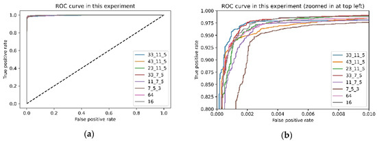
Figure 5.
Receiver operating characteristic (ROC) curve about this experiment: (a) original ROC curve; (b) zoomed ROC curve.
It is not difficult to find from Table 5 that although these results are not much different, the larger-sized convolution kernel’s performance is slightly better in the first convolution group. The convolution kernel size is different; the receptive field of the convolution kernel is also other. For the data used in this experiment, a larger size convolution kernel is more suitable for this task than a smaller size convolution kernel.
On the other hand, when the number of convolution kernels in each layer is 64 or 16, the model’s performance has declined somewhat. The reason for this experimental phenomenon is that the number of convolution kernels is positively correlated with the learnable parameters in the model. The fewer the number of convolution kernels, the fewer the model’s learnable parameters, which leads to the model not being able to extract features effectively. Also known as the underfitting state.
Furthermore, the number of convolution kernels also has a positive correlation with the time spent training the model. Especially when the number of convolution kernels in each layer is 64, the time spent training the model is nearly 15 min. Considering the accuracy, sensitivity, and Youden’s index, the better combinations are the second to the fifth set of records in Table 5.
Moreover, from the ROC curves Figure 5, we can quickly know that the better combinations are the second combination in this experiment. Coincidentally, the receptive field of the convolution kernel is about 0.1 s of ECG signal when the kernel size is 33 because the sampling rate of the ECG is 360, and the QRS complexes of PVC are unusually long (typically >120 ms). In future work, we will study whether there is a relationship between the kernel size and the QRS duration of PVC.
3.2. Experiment 2: The Performance of CNN with a Different Number of Layers
With the popularity of CNN, the number of convolutional layers in each network is continually increasing, such as AlexNet (5), VGGNet16(13), ResNet50(49). The emergence of batch normalization and residual structure solves the vanishing gradient problem that makes the previous CNN challenging. Considering the marginal effects and the efficiency of the proposed model, we performed three tests. Figure 6 illustrates the basic structure of the model used in the three experiments. The configuration in this experiment is the same as the previous experiment. Moreover, Table 6 gives the results.
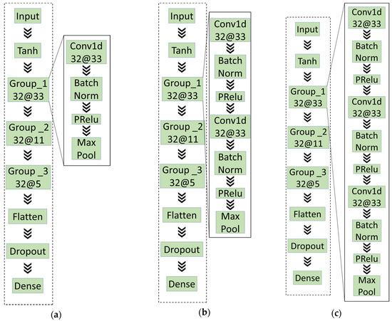
Figure 6.
The basic structure of the models in experiment 2: (a) A convolutional layer in each convolutional; (b) two convolutional layers in each convolutional; (c) three convolutional layers in each convolutional.
Table 6.
The details and results of the varying size and number of kernels.
The experimental records in Table 6 illustrate that the number of convolutional layers is not as significant as possible, which is the same as the existing prior knowledge. For example, the network with the first structure requires shorter training time than the third structure and better in some index, such as accuracy.
Besides, the number of layers is usually an essential factor that affects the complexity of the model. High-complexity models may have over-fitting problems during the training process, while low-complexity models may have under-fitting questions. Those models with too high or too low complexity have difficulty and time-consuming training. Therefore, choosing a moderately complex model can speed up the training process and make training easier.
3.3. Experiment 3: Test the Batch Size’s Effect on Detecting PVC
Batch size is a very critical parameter and affects the performance of the neural networks. Too large or too small batch size is not appropriate. The larger batch size can reduce the training time and improve the stability of the structure. However, the smaller batch size can enhance the generalization ability of the model. To balance the generalization ability of the model and training time, we tested a series of batch sizes. Table 7 shows the results of this experiment.
Table 7.
Test the batch size’s effect in detecting PVC.
According to the experimental results in Table 7, we can find this rule that the relationship between training time and batch size is negatively correlated. Further, as the batch size keeps getting bigger, the training time is decreasing more and more slowly. Considering the training time, accuracy, and other indicators, we set the batch size in subsequent experiments to 512. After deploying the trained model, increasing the batch size can predict multiple heartbeats at the same time within the allowable range of video memory. This characteristic can significantly improve the efficiency of PVC detection in practical applications.
3.4. Experiment 4: Test the Activation Functions (Sigmoid, Tanh) Used to Normalize the Input Data
Considering the waveform of the ECG, normalizing the input data can improve the performance of the proposed model. Because the amplitude of the R wave is several times that of the other waves, we adopted the Sigmoid and Tanh function to normalize the input data. The Tanh function can normalize the input data between –1 and 1. The Sigmoid function can normalize the input data between 0 and 1. The difference is that the overall slope of Tanh is greater. Table 8 shows the results of this experiment.
Table 8.
Test the activation functions.
The waveform of the ECG is very special. The amplitude of QRS complexes usually is much higher than the remaining wave. As shown in Figure 7, the points on the unnormalized waveform are mostly near the straight line with y = –1.0, and only a few moments deviate seriously. To solve this problem, we tried two activation functions (Tanh and Sigmoid) to normalize the input ECG. Figure 7 shows the normalized waveform of the ECG. The experimental results in Table 8 show that the suitable activation functions (Tanh) used to normalize the input ECG can slightly improve the model’s performance. Nevertheless, inappropriate activation functions (Sigmoid) have a negative impact. The advantage of the Tanh function is that the value range of the normalized data is between –1 and 1, and the average is 0, unlike sigmoid, which is 0.5.
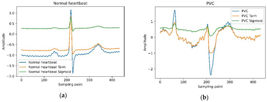
Figure 7.
Tanh and Sigmoid normalize the waveform of a normal heartbeat and PVC.
3.5. Experiment 5: Employ CNN to Identify PVC with Scheme 2 and Scheme 3
As we all know, it is a common practice to distribute training and test sets in the proportion of 9:1 or 4:1 in deep learning. This experiment re-divides the data set according to Scheme 2 and Scheme 3, described in Table 2. After obtaining the training set and test set, this experiment employs the proposed model. Figure 8 shows the confusion matrix of each scheme. Table 9 shows the results of this experiment and comparisons with the consequence of Scheme 1 and previous studies.
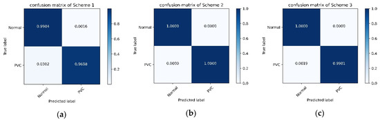
Figure 8.
The confusion matrix of each scheme: (a) confusion matrix of Scheme 1; (b) confusion matrix of Scheme 2; (c) confusion matrix of Scheme 3.
Table 9.
Employ the proposed model with Scheme 2 and Scheme 3.
The above experiments 1–4 confirmed the architecture and parameters of our proposed model. In Experiment 5, to evaluate the proposed model’s performance in this situation: the number of samples in the training set is more than the test set. We employed the proposed model with Scheme 2 and 3. According to Table 9 and Figure 8, the proposed model’s performance is unexpected, and the indicators are full marks with Scheme 2. The convolutional neural network is a class of deep learning technology. In deep learning, the number of samples used to train is generally more than that used for testing. In this case, the performance of the proposed method is remarkable.
Compared with the literature 9, 11, 12, and 13, the performance of the proposed method in Scheme 1 is better in all indicators. Additionally, the proposed method does not rely on professional knowledge to manually extract features. Next, the proposed method can directly predict the heartbeats’ category in the MIT-BIH arrhythmia database without denoising.
For literature 17, the performance of the proposed method in Scheme 1 is bleak in all indicators. The literature 17 is based on a patient-independent separation approach to divide the training set and test set. This separation approach follows a principle that the same subject’s heartbeats cannot appear in both training and test sets. The experiment in literature 17 considered 10% of heartbeat in the MIT-BIH arrhythmia database for training and 90% as the test set, similar to Scheme 3. The proposed method’s performance in Scheme 3 is almost close to full marks and is better than literature 17.
Compared with the literature 23, 24, and 25, the proposed method’s results are better. In the proposed plan, the process of extracting features and recognizing heartbeats are performed simultaneously. Finally, the proposed model can directly identify heartbeats in the MIT-BIH arrhythmia database. On the contrary, literature 23 used wavelet function to transform the heartbeat before training the model; before training the classifier model, literature 24 and 25 must first train the feature extraction network. In summary, our method has reached the most advanced level compared with other studies.
4. Conclusions
In this study, we successfully apply a model based on the one-dimensional convolutional neural network to recognize PVC and worked highly efficiently by using the raw ECG data without complex signal preprocessing such as denoising. The experimental results show that the classification effect achieved by the proposed method is significantly better than the morphological-based method and other methods. Additionally, according to Table 9, applying more ECG data can improve the performance of the proposed method. However, the annotated ECG data is hard to come by. In future works, we plan to use the generative adversarial networks (GAN) to deal with insufficient data. Next, we hope to tap the potential of our approach to classify many different types of heartbeats simultaneously. Lastly, we plan to deploy our proposed method on cloud servers or wearables to help doctors and patients in developing countries or remote regions.
Author Contributions
Conceptualization, X.C.; data curation, X.W. and J.G.; formal analysis, X.W.; methodology, J.Y., X.C. and J.G.; project administration, X.C.; resources, J.Y.; software, J.G.; visualization, J.G.; writing—original draft, X.W.; writing—review and editing, J.Y. and X.C. All authors have read and agreed to the published version of the manuscript.
Funding
This research received no external funding.
Conflicts of Interest
The authors declare no conflict of interest.
References
- Zhang, Y.; Cong, H.; Man, C.; Su, Y.; Sun, H.; Yang, H.; Guo, Z. Risk factors for cardiovascular disease from a population-based screening study in Tianjin, China: A cohort study of 36,215 residents. Ann. Transl. Med. 2020, 8, 444. [Google Scholar] [CrossRef]
- Gerstenfeld, E.P.; De Marco, T. Premature ventricular contractions. Circulation 2019, 140, 624–626. [Google Scholar] [CrossRef] [PubMed]
- Park, K.M.; Im, S.I.; Chun, K.J.; Hwang, J.K.; Park, S.J.; Kim, J.S.; On, Y.K. Asymptomatic ventricular premature depolarizations are not necessarily benign. EP Eur. 2015, 18, 881–887. [Google Scholar] [CrossRef] [PubMed]
- Zipes, D.P.; Libby, P.; Bonow, R.O.; Mann, D.L.; Tomaselli, G.F. Braunwald’s Heart Disease E-Book: A Textbook of Cardiovascular Medicine; Elsevier Health Sciences: Philadelphia, PA, USA, 2018. [Google Scholar]
- Manikandan, M.S.; Ramkumar, B.; Choudhary, T.; Deshpande, P.S. Robust detection of premature ventricular contractions using sparse signal decomposition and temporal features. Health Technol. Lett. 2015, 2, 141–148. [Google Scholar] [CrossRef] [PubMed]
- Abadi, M.; Barham, P.; Chen, J.; Chen, Z.; Davis, A.; Dean, J.; Devin, M.; Ghemawat, S.; Irving, G.; Isard, M. Tensorflow: A system for large-scale machine learning. arXiv 2016, arXiv:1605.08695. [Google Scholar]
- Jun, T.J.; Park, H.J.; Minh, N.H.; Kim, D.; Kim, Y. Premature ventricular contraction beat detection with deep neural networks. In Proceedings of the 15th IEEE International Conference on Machine Learning and Applications (ICMLA), Anaheim, CA, USA, 18–20 December 2016; pp. 859–864. [Google Scholar] [CrossRef]
- Hadia, R.; Guldenring, D.; Finlay, D.D.; Kennedy, A.; Janjua, G.; Bond, R.; McLaughlin, J. Morphology-based detection of premature ventricular contractions. In 2017 Computing in Cardiology (CinC); IEEE: Rennes, France, 2017; pp. 1–4. [Google Scholar] [CrossRef]
- Atanasoski, V.; Ivanovic, M.D.; Marinkovic, M.; Gligoric, G.; Bojovic, B.; Shvilkin, A.V.; Petrovic, J. Unsupervised classification of premature ventricular contractions based on R-R interval and heartbeat morphology. In Proceedings of the 14th Symposium on Neural Networks and Applications (NEUREL), Belgrade, Serbia, 20–21 November 2018; pp. 1–6. [Google Scholar] [CrossRef]
- Junior, E.A.; Valentim, R.A.D.M.; Brandão, G.B. Real-time premature ventricular contractions detection based on Redundant Discrete Wavelet Transform. Res. Biomed. Eng. 2018, 34, 187–197. [Google Scholar] [CrossRef]
- De Oliveira, B.R.; De Abreu, C.C.E.; Duarte, M.A.Q.; Filho, J.V. Geometrical features for premature ventricular contraction recognition with analytic hierarchy process based machine learning algorithms selection. Comput. Methods Programs Biomed. 2019, 169, 59–69. [Google Scholar] [CrossRef]
- Lynggaard, P. Detecting premature ventricular contraction by using regulated discriminant analysis with very sparse training data. Appl. Artif. Intell. 2018, 33, 229–248. [Google Scholar] [CrossRef]
- Sokolova, A.; Markelov, O.; Bogachev, M.; Uljanitski, Y. Multi-parametric algorithm for premature ventricular contractions detection and counting. AIP Conf. Proc. 2019, 2140, 020074. [Google Scholar] [CrossRef]
- Rizal, A.; Wijayanto, I. Classification of Premature Ventricular Contraction based on ECG Signal using Multiorder Rényi Entropy. In Proceedings of the 2019 International Conference of Artificial Intelligence and Information Technology (ICAIIT), Yogyakarta, Indonesia, 13–15 March 2019; pp. 225–229. [Google Scholar] [CrossRef]
- Chen, H.; Bai, J.; Mao, L.; Wei, J.; Song, J.; Zhang, R. Automatic Identification of Premature Ventricular Contraction Using ECGs. In Proceedings of the 2019 International Conference on Health Information Science (HIS), Xi’an, China, 18–20 October 2019; pp. 143–155. [Google Scholar] [CrossRef]
- Mazidi, M.H.; Eshghi, M.; Raoufy, M.R. FPGA implementation of wearable ECG system for detection premature ventricular contraction. Int. J. COMADEM 2019, 22, 51–59. [Google Scholar]
- Mazidi, M.H.; Eshghi, M.; Raoufy, M.R. Detection of premature ventricular contraction (PVC) using linear and nonlinear techniques: An experimental study. Clust. Comput. 2019, 23, 759–774. [Google Scholar] [CrossRef]
- Allami, R. Premature ventricular contraction analysis for real-time patient monitoring. Biomed. Signal. Process. Control. 2019, 47, 358–365. [Google Scholar] [CrossRef]
- Chen, Z.; Xu, H.; Luo, J.; Zhu, T.; Meng, J. Low-power perceptron model based ECG processor for premature ventricular contraction detection. Microprocess. Microsyst. 2018, 59, 29–36. [Google Scholar] [CrossRef]
- Jeon, E.; Jung, B.K.; Nam, Y.; Lee, H. Classification of premature ventricular contraction using error back-propagation. KSII Trans. Internet Inf. Syst. 2018, 12, 988–1001. [Google Scholar] [CrossRef]
- Zhou, X.; Zhu, X.; Nakamura, K.; Mahito, N.P. Premature ventricular contraction detection from ambulatory ECG using recurrent neural networks. In Proceedings of the 40th Annual International Conference of the IEEE Engineering in Medicine and Biology Society (EMBC), Honolulu, HI, USA, 18–21 July 2018; pp. 2551–2554. [Google Scholar] [CrossRef]
- Zhao, Z.; Wang, X.; Cai, Z.; Li, J.; Liu, C.P. PVC Recognition for wearable ECGs using modified frequency slice wavelet transform and convolutional neural network. In Proceedings of the 2019 Computing in Cardiology (CinC), Biopolis, Singapore, 8–11 September 2019; pp. 1–4. [Google Scholar] [CrossRef]
- Li, Q.; Liu, C.; Li, Q.; Shashikumar, S.P.; Nemati, S.; Shen, Z.; Clifford, G.D. Ventricular ectopic beat detection using a wavelet transform and a convolutional neural network. Physiol. Meas. 2019, 40, 055002. [Google Scholar] [CrossRef] [PubMed]
- Gordon, M.G.; Williams, C.M. PVC detection using a convolutional autoencoder and random forest classifier. In Proceedings of the Pacific Symposium on Biocomputing 2019, Kohala Coast, HI, USA, 3–7 January 2019; pp. 42–53. [Google Scholar] [CrossRef]
- Rahhal, M.M.A.; Ajlan, N.A.; Bazi, Y.; Hichri, H.A.; Rabczuk, T. Automatic premature ventricular contractions detection for multi-lead electrocardiogram signal. In Proceedings of the IEEE International Conference on Electro/Information Technology (EIT), Rochester, MI, USA, 3–5 May 2018; pp. 169–173. [Google Scholar] [CrossRef]
- Hoang, T.; Fahier, N.; Fang, W.C. Multi-leads ECG premature ventricular contraction detection using tensor decomposition and convolutional neural network. In Proceedings of the BioCAS 2019—Biomedical Circuits and Systems Conference, Nara, Japan, 17–19 October 2019; pp. 1–4. [Google Scholar] [CrossRef]
- Liu, Y.; Huang, Y.; Wang, J.; Liu, L.; Luo, J. Detecting premature ventricular contraction in children with deep learning. J. Shanghai Jiaotong Univ. 2018, 23, 66–73. [Google Scholar] [CrossRef]
- Moody, G.; Mark, R. The impact of the MIT-BIH arrhythmia database. IEEE Eng. Med. Biol. Mag. 2001, 20, 45–50. [Google Scholar] [CrossRef] [PubMed]
- Goldberger, A.L.; Amaral, L.A.N.; Glass, L.; Hausdorff, J.M.; Ivanov, P.C.; Mark, R.G.; Mietus, J.E.; Moody, G.B.; Peng, C.K.; Stanley, H.E. PhysioBank, PhysioToolkit, and PhysioNet: Components of a new research resource for complex physiologic signals. Circulation 2000, 101, e215–e220. [Google Scholar] [CrossRef]
- Pan, J.; Tompkins, W. A Real-Time QRS Detection Algorithm. IEEE Trans. Bio-Med. Eng. 1985, 32, 230–236. [Google Scholar] [CrossRef]
- Lin, C.C.; Chang, H.Y.; Huang, Y.H.; Yeh, C.Y. A novel wavelet-based algorithm for detection of QRS complex. Appl. Sci. 2019, 9, 2142. [Google Scholar] [CrossRef]
- Chen, C.L.; Chuang, C.T. A QRS detection and R point recognition method for wearable single-lead ECG devices. Sensors 2017, 17, 1969. [Google Scholar] [CrossRef] [PubMed]
- Chen, A.; Zhang, Y.; Zhang, M.; Liu, W.; Chang, S.; Wang, H.; He, J.; Huang, Q. A real time QRS detection algorithm based on ET and PD controlled threshold strategy. Sensors 2020, 20, 4003. [Google Scholar] [CrossRef] [PubMed]
- Garbin, C.; Zhu, X.; Marques, O. Dropout vs. batch normalization: An empirical study of their impact to deep learning. Multimedia Tools Appl. 2020, 79, 12777–12815. [Google Scholar] [CrossRef]
- He, K.; Zhang, X.; Ren, S.; Sun, J. Delving Deep into Rectifiers: Surpassing Human-Level Performance on ImageNet Classification. In Proceedings of the 2015 IEEE International Conference on Computer Vision (ICCV), Santiago, Chile, 7–13 December 2015; pp. 1026–1034. [Google Scholar] [CrossRef]
Publisher’s Note: MDPI stays neutral with regard to jurisdictional claims in published maps and institutional affiliations. |
© 2020 by the authors. Licensee MDPI, Basel, Switzerland. This article is an open access article distributed under the terms and conditions of the Creative Commons Attribution (CC BY) license (http://creativecommons.org/licenses/by/4.0/).