Development of Fail-Safe Algorithm for Exteroceptive Sensors of Autonomous Vehicles

Abstract

This paper presents a fail-safe algorithm for the exteroceptive sensors of autonomous vehicles. The proposed fault diagnosis mechanism consists of three parts: (1) fault detecting by a duplication-comparison method, (2) fault isolating by possible area prediction and (3) in-vehicle sensor fail-safes. The main ideas are the usage of redundant external sensor pairs, which estimate the same target, whose results are compared to detect the fault by a modified duplication-comparison method and the novel fault isolation method using target predictions. By comparing the estimations of surrounding vehicles and the raw measurement data, the location of faults can be determined whether they are from sensors themselves or a software error. In addition, faults were isolated by defining possible areas where existing sensor coordinates could be measured, which can be predicted by using previous estimation results. The performance of the algorithm has been tested by using offline vehicle data analysis via MATLAB. Various fault injection experiments were conducted and the performance of the suggested algorithm was evaluated based on the time interval between injection and the detection of faults.

1. Introduction

Health monitoring or fault-tolerant control systems is one of the most essential elements for control systems. When an automated system operates, there is always a chance that system failure occurs. It can be broken hardware (e.g., crack in the bolt cutting it), deficiency in software or an error in sensors. This is critical because these somewhat trivial breakdowns can cause dangerous situations. Therefore, there have been many studies on fault-detection and fault-tolerant control systems.

Sensing and the perception of the environment are major challenging technologies for the high-level automated vehicles. Until now, exteroceptive sensors—which are used to sense the surroundings around autonomous vehicles—such as a camera, an automotive radar or LiDAR (Light Detection and Ranging), play an important role in this domain. According to [1], using fusion of vision, radar and a LiDAR system is the most common approach to achieve robust situation awareness. Therefore, this research questions how to achieve robustness of these sensors which has become an important topic. To improve vehicles’ integrity, many studies using information of vehicle sensors and actuators have already been conducted. For example, one of the previous study uses the Mahalanobis distance and chi square as a threshold to detect the fault [2]. The fusion of odometry with DGPS (Differential Global Positioning System), IMU (Inertial measurement uni) and magnetic field sensors is also investigated to develop fault-tolerant 3D localization system [3]. Although there have been extensive studies on the sensor integrity of vehicle sensors, only a few of them have focused on the reliability of environment perception sensors such as radar, camera, and LiDAR. The main contribution of this paper is the use of redundant external sensor pairs, which estimate the same target, whose results are compared to detect the fault.

Health monitoring and fault-tolerant control systems can be divided into three main processes: fault detection, fault diagnosis and fault-tolerant control. First of all, fault should be detected. However, it is not an easy task because forecasting every possible fault and its effect is almost impossible. Nevertheless, there exist several methods to analyze faults and their effects. One of these methods is Fault Propagation Analysis (FPA) using an FMEA (Failure Modes and Effects Analysis) matrix [4]. This divides the system into parts that perform the same function and analyzes how failure of one element can affect the entire system. Blank [4] applied the method to the three-level valve control system and it is usually applied to hardware systems.

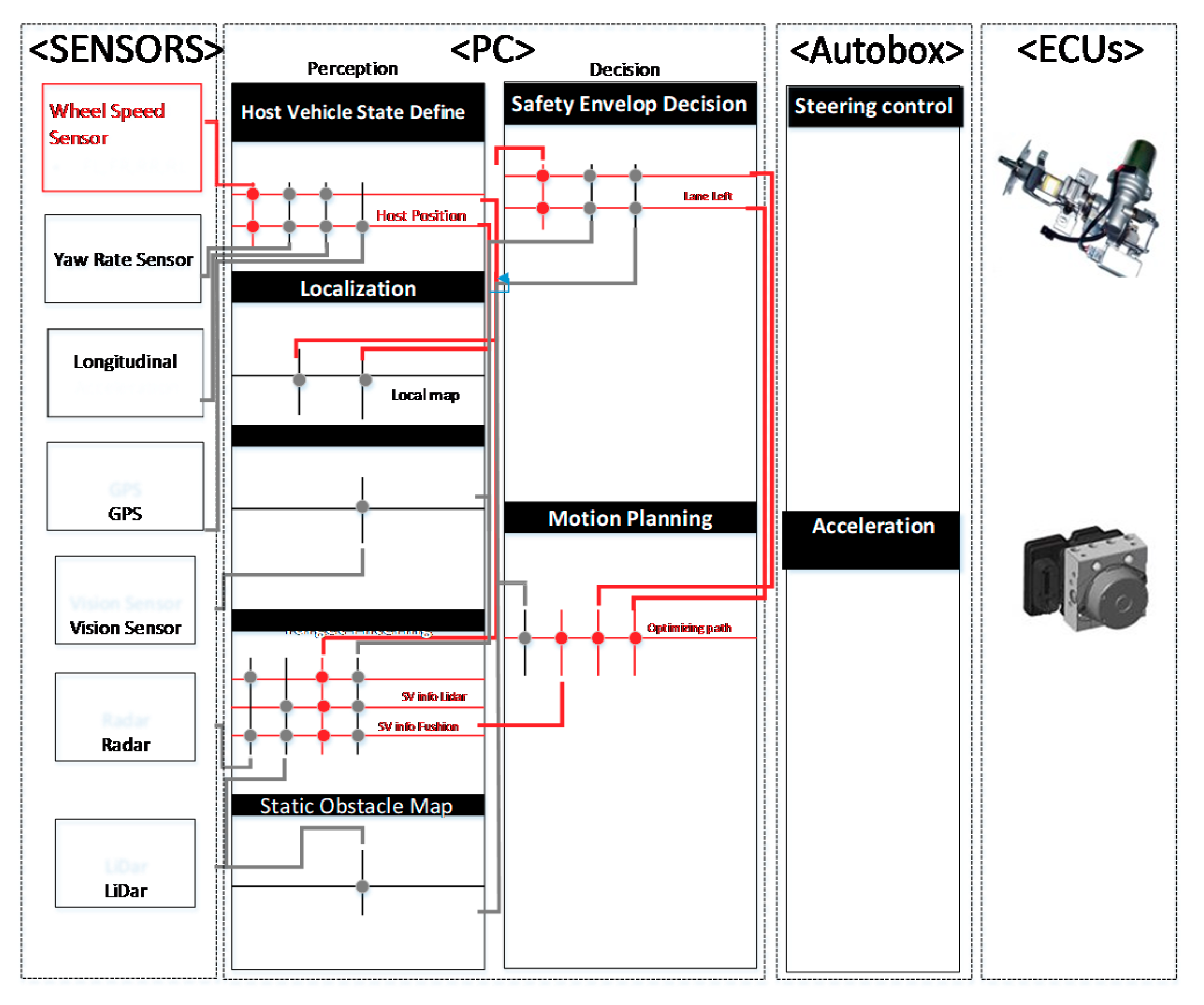
In this paper, the method was applied to the software of an autonomous driving system in order to see how one of the sensors’ failures affects the entire autonomous driving system. An example is described in Figure 1. However, pioneers in this field have figured out two effective ways to investigate how sensor failure affects the system—using limit checking [5] and using redundancy relations [6]. Both generate features from output signals of the control system, but the differences lie between whether they use direct signal properties or redundant relations. Second, faults are isolated and their failure effects are classified into hazard classes in a fault-diagnosis process. This can be applied to other kinds of systems such as fuzzy systems and time delay systems by isolating fault with predictions of each boundary of interest. There are also a lot of methods to classify fault effects, but they were not investigated deeply in this paper. Lastly, after faults are detected and evaluated, fault-tolerant control should be designed. Several fault-tolerant control designs were introduced in [6]. The Takagi-Sugeno (T-S) model approach was presented to represent the nonlinear dynamic of the induction motor which is subject to speed sensor faults and unknown bounded disturbance [7]. Chibani et al. [8] investigated the problem of fault detection filter designs for discrete-time polynomial fuzzy systems with faults and unknown disturbances.

2. Background

To design fail-safe algorithms for a system, not only is it important to know the mechanisms of how the failure occurs but also to choose an appropriate algorithm among the various fault detection mechanisms that have been introduced. This section describes the role of external sensors, radar sensor and LiDAR in the autonomous driving system and introduces the fault-error failure chain and the duplication-comparison method for designing the fail-safe algorithm.

2.1. Architecture for Autonomous Driving System and External Sensors

In our autonomous driving system, automotive radar sensor and laser scanner play a key role in localizing and perceiving the environment as described in Figure 2. Radar points wandering on the edges of surrounding vehicles were used to estimate the position and the overall behavior of surrounding vehicles. In addition, LiDAR point clouds whose shapes are similar to the road boundary (i.e., curbstones and guardrails) or vehicles were used for map-based localization or vehicle tracking. LiDAR point clouds also provide information on the static obstacles by overlapping previously measured data clouds.

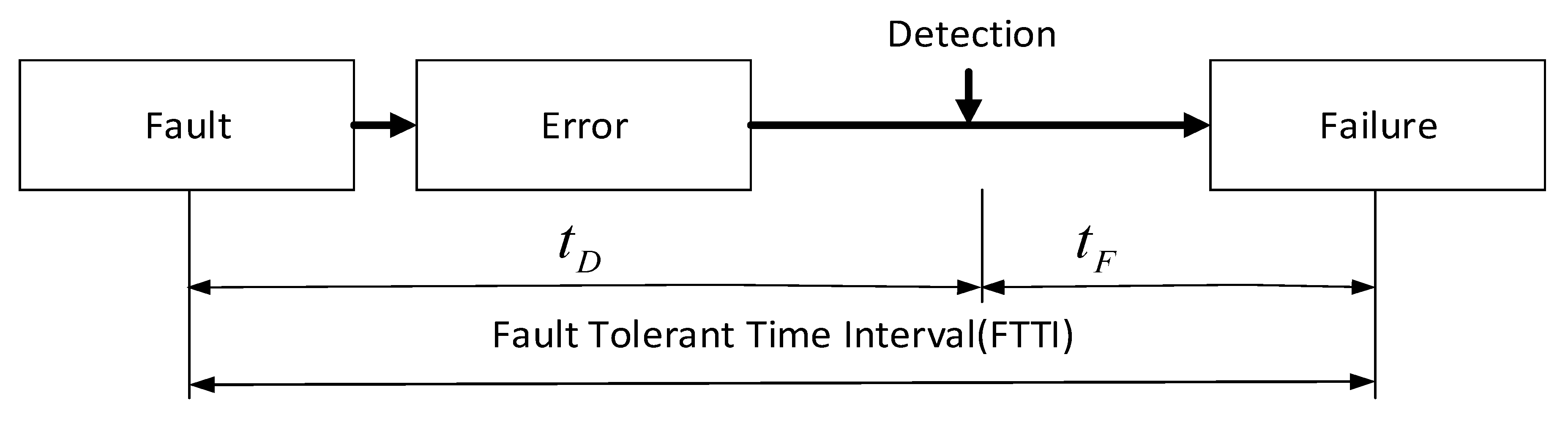
2.2. Fault-Error Failure Chain and Safety Related Time Intervals

To secure the fail-safety of a system, it is important to be aware of fault-error failure chain. Fault is a small deviation on one or multiple components which could cause system error or failure. Isermann [5] defined a fault as “an unpermitted deviation of at least one characteristic property (feature) of the system from the acceptable, usual, standard condition”. When faults occur, they propagate through the system and cause error and failure. Benso et al. [9] defines an error as a deviation from accuracy or correctness and Isermann [5] defines failure as a permanent interruption of a system’s ability to perform a required function under specified operating conditions in his book. When Alrat et al. [10] conducted a fault injection experiment to evaluate the dependability for their delta-4 architecture, they classified propagating stages into seven categories. (1) Faults are not activated and cause no significant effect on the system. (2) Faults are activated as errors. (3) Errors are detected. (4) Errors are tolerated without detection. (5) Errors cause failure of the detection. (6) Errors are detected and tolerated. (7) Errors are detected but not tolerated. For the functional fail-safety algorithm to perform properly, detecting faults before they cause a fatal system failure is important. The goal of this study is to find the faulty behavior of radar and laser scanners before they cause malfunction of the autonomous driving system. So, two definitions about time are defined in Figure 3—time between fault injected and detected ($t_D$), and time that causes a failure after the detection ($t_F$).

2.3. Duplication Comparison

There have been many studies on detecting sensor fault, especially by using redundant sensor pairs. For example, Sebastian et al. [11] combined three different sensors to estimate the exact location of a mobile robot. They exploited ultrasound sensor, laser scanner and camera systems. By combining model-based estimations, the failure of each sensor was compensated. Ricquebourg et al. [12] also used three different sensors for the detection of a deviated sensor. This paper also used redundant sensor pairs and modified a duplication-comparison method, which was introduced in Bader’s work [13] to detect sensor failure. Duplication comparison is a method that utilizes at least two redundant units providing the same results and compares them to find the abnormal behavior of system. Bader et al. [13] used various sensors as inputs and measurement sets of two identical branches of a Kalman filter, which estimated the location of the vehicle. When the result of one branch would be different from the other, the input and measurement sensor pairs were compared to find whether faults were from sensors themselves or a software error. After faults were confirmed to be from the hardware, residuals of each branch were investigated and faults were isolated. In this work, a radar sensor and laser scanner were used as redundant sensor pairs. In addition, target-tracking filters which estimate the overall behavior of surrounding vehicles were used as two identical branches and their positions were compared.

3. Fail-Safe Algorithm for Exteroceptive Sensors of Autonomous Vehicle

The proposed exteroceptive sensor fail-safe algorithm is activated when surrounding vehicles ride alongside the ego vehicle as shown in Figure 4. After the existence of surrounding vehicles is confirmed, the algorithm chooses the closest eight targets and conducts a fault diagnosis. A fault diagnosis uses three sensors, in-vehicle sensors, a radar sensor and laser scanner, and consists of three parts: (1) fault detecting by duplication-comparison method, (2) fault isolating by possible area prediction and (3) in-vehicle sensor fail-safes. The mechanism to find the faults uses hypothesis testing. Details on the algorithm were described in this section.

3.1. Target Classification

If the algorithm is activated, the closest eight surrounding vehicles are chosen and classified based on the distance between the ego vehicle’s center position and 12 measurement points on the edges of the target vehicles. The eight areas are defined: (1) rear-left of ego vehicle, (2) left side of ego vehicle, (3) front-left of ego vehicle, (4) front of ego vehicle, (5) front-right of ego vehicle, (6) right side of ego vehicle, (7) rear-right of ego vehicle and (8) rear of ego vehicle.

3.2. Target Tracking with Radar Sensor

The eight classified targets’ overall behaviors are estimated and represented by each sensor. In the case of the radar sensor, it is hard to estimate target vehicles’ position because radar measurements are wandering on the physical surface of the vehicle. Therefore, 12 measurement points are defined on the edges of vehicle and used as a measurement model. The measurements are updated 12 times to estimate target vehicles’ states and the model that has the highest possibility is selected by the interacting multiple model filter. In addition, the process model which represents the vehicle’s movement with no slip ($\beta \approx 0$) assumption is used. The discretized version of the process model is described as follows:

$$\begin{gathered} \mathrm{x}[k+1]={\left[\begin{array}{cccc}\begin{array}{cccc}{f}_1& f_2& f_3& f_4\end{array}& f_5& f_6& f_7\end{array}\right]}^T+\mathrm{w}[k] \\ \begin{array}{c}\mathrm{where}\hfill \\ {\mathrm{f}}_1=-(\frac{{\gamma }_{host}(x{\gamma }_{host}-v\sin (\theta ))}{2}-\frac{a\cos (\theta )}{2}\hfill \\ +\frac{\gamma v\sin (\theta )}{2}+\frac{a_{host}}{2}-\frac{y\dot{\gamma }}{2})\Delta T^2\\ +(y{\gamma }_{host}-v_{host}+v\cos (\theta ))\Delta T+x\\ {\mathrm{f}}_2=-(\frac{a\sin (\theta )}{2}+\frac{\gamma v\cos (\theta )}{2}+\frac{x\dot{\gamma }}{2}\hfill \\ -\frac{{\gamma }_{host}(y{\gamma }_{host}-v_{host}+v\cos (\theta ))}{2})\Delta T^2\\ -(x{\gamma }_{host}-v\sin (\theta ))\Delta T+y\\ {\mathrm{f}}_3=\frac{\dot{\gamma }}{2}\Delta T^2+\gamma \Delta T+\theta \hfill \\ {\mathrm{f}}_4=-\frac{a{k}_a}{2}\Delta T^2+a\Delta T+v\hfill \\ {\mathrm{f}}_5=-\frac{k_{\dot{\gamma }}\dot{\gamma }}{2}\Delta T^2+\dot{\gamma }\Delta T+\gamma \hfill \\ {\mathrm{f}}_6=\frac{a}{2}(k_a{}^2\Delta T^2-2k_a\Delta T+2)\hfill \\ {\mathrm{f}}_7=\frac{\dot{\gamma }}{2}(k_{\dot{\gamma }}{}^2\Delta T^2-2k_{\dot{\gamma }}\Delta T+2)\hfill \\ \mathrm{w}[k]\sim (0,\mathrm{W}[k\left]\right)\end{array} \end{gathered}$$

(1)

$x$ and $y$ denote the relative position at the x-axis and y-axis, $\theta$ denotes the relative yaw angle, $v$ denotes the velocity, $\gamma$ denotes the yaw rate, $a$ denotes the acceleration, and $\dot{\gamma }$ denotes the yaw acceleration. More detailed description is available in [14].

3.3. Target Tracking with LiDAR

Tracking the target vehicle with LiDAR sensors also consists of data-processing parts and a filtering part. In data-processing parts, vehicle-like LiDAR point clouds were selected and the position and yaw of vehicle were extracted from the shapes of the LiDAR point clouds. In order to do this, the extracted vehicle-shape data points, which detect the same object, were clustered. To classify LiDAR point clouds, the EMST(Euclidean Minimum Spanning Tree) method and 0.5 by 0.5 of a lateral and longitudinal grid were implemented. [15] describes the details of this algorithm. Shape extraction is conducted by estimating the rear-center of the vehicle. For this the Random Sample Consensus (RANSAC) algorithm is used. For the detailed description see [16]. The extended Kalman filter is used to estimate target vehicles’ overall behavior by using extracted vehicles’ position and angle as measurements. The process model is the same as the model for radar target-tracking systems which indicates that both sensors estimate the same states of targets. The state vector is described as follows:

$${\mathrm{x}}_n={\left[x_n y_n {\theta }_n v_{x,n} {\gamma }_n a_n {\dot{\gamma }}_n\right]}^T$$

(2)

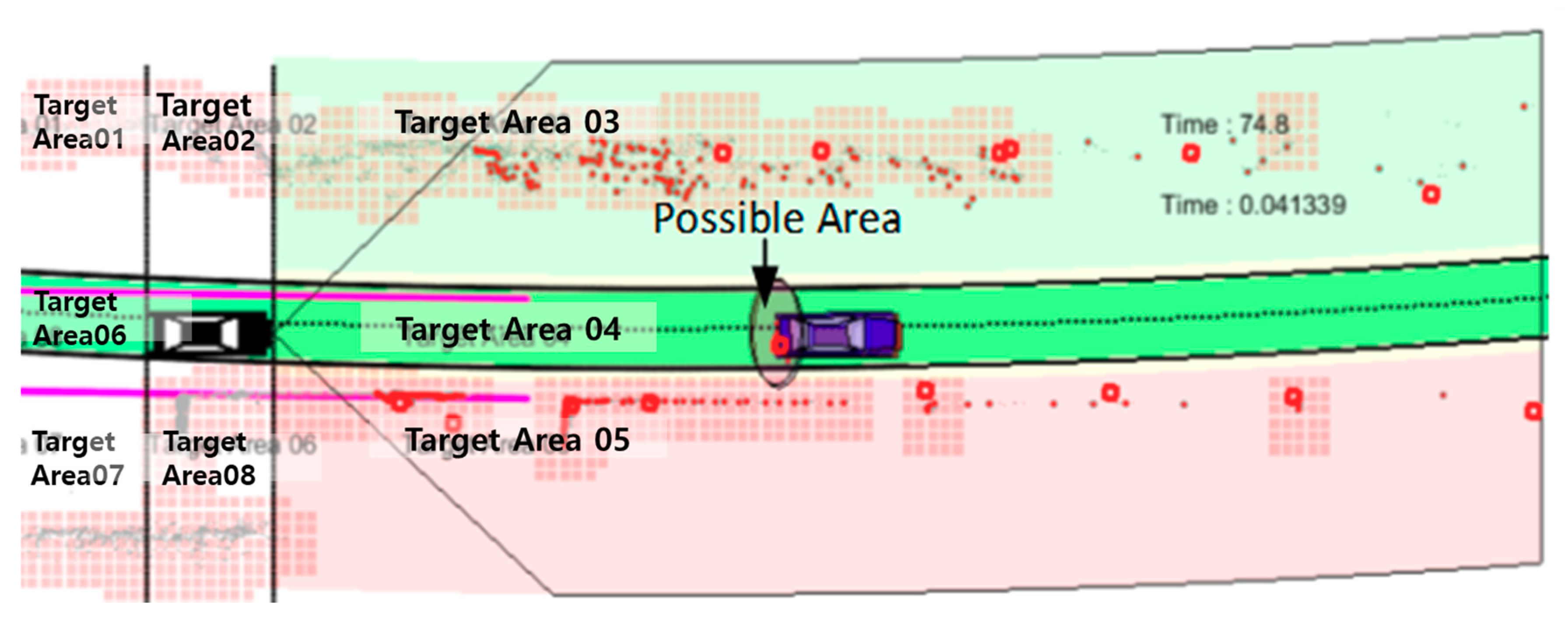
3.4. Possible Area Prediction

Automotive radar and LiDAR offer the relative range and angle of the detected object based on the host vehicle’s position and heading by interpreting signals that are reflected on the surface of the objects. Therefore, the measurements can be expressed on the host vehicle’s body-fixed coordinate by simply changing the polar coordinate into a Euclidian coordinate. The possible area defined to isolate fault in this paper is an area where radar and LiDAR measurements should exist. For example, if the target vehicle is in the front of ego vehicle, the rear edge of the target vehicle would be detected and the rear side of the target vehicle would become a possible area. Possible area can be calculated by predicting future behavior of the estimated surrounding targets at the previous. For example, the position of target vehicle at k^th step can be predicted by the estimation results at k-1^th, k-2^nd, k-3^rd, etc. However, since the host vehicle’s body-fixed coordinate changes every iteration as the host vehicle moves, the position of the predicted target vehicle should be rotated and transferred to be displayed on a new host vehicle’s body-fixed coordinate as illustrated in Figure 5.

3.4.1. Target Prediction

A conventional T-S observer is designed with unmeasured premise variables, whereas most existing works using fuzzy models consider observers with measurable premise variables [17]. As a consequence, if premise variables are not available for measurements, the target’s potential future behavior can be predicted by a linearized Kalman filter using a path-following model-based desired yaw rate as a virtual measurement. The desired yaw rate used for the prediction represents a driver model that maintains the current behavior in the near future and keeps the lane in the far-off future, and is generated by an error state feedback term and a feedforward term of road curvature. A path-following model in [18] is described as follows.

$${\dot{\mathrm{x}}}_{\mathrm{e}}={\mathrm{F}}_{\mathrm{e}}·{\mathrm{x}}_{\mathrm{e}}+{\mathrm{G}}_{\mathrm{e}}·{\gamma }_{\mathrm{des}}{+ \mathrm{G}}_{\mathrm{w}}·a_2$$

(3)

3.4.2. Host Vehicle Filter

Wang et al. adopted the Affine Force-Input (AFI) model in order to preserve the linear relationship between the input and the model states [19]. Although this approach allows the simplified formation of the rear-wheel latera force, it is hard to represent the driver’s intention and the vehicle’s planar behavior. In order to reflect this, the host vehicle’s velocity, longitudinal acceleration, and yaw rate are to be estimated using a Kalman filter—described below.

$$\begin{array}{l}x[k+1]=F[k]·x[k]+w[k]\\ z[k]=Hx[k]+v[k]\\ \mathrm{where}\\ F=\left[\begin{array}{cccc}1& 0& \Delta t& 0\\ 0& 1& 0& \Delta t\\ 0& 0& 1& 0\\ 0& 0& 0& 1\end{array}\right] \\ H=\left[\begin{array}{cccc}1& 0& 0& 0\\ 0& 1& 0& 0\\ 0& 0& 1& 0\\ 0& h_{42}& 0& h_{44}\end{array}\right]\\ h_{42}=\frac{2l_f{}^2{C}_f+2l_r{}^2{C}_r}{2l_f{C}_{f}v} \\ h_{44}=\frac{I_z}{2l_f{C}_f}\end{array}$$

(4)

The detailed description of the host vehicle filter can be found in [20].

The host vehicle’s body-fixed coordinate change at every step as:

$$\left(\begin{array}{l}dx\\ dy\\ d\theta \end{array}\right)=\left(\begin{array}{l}(vdt+ad{t}^2)\cos (\gamma dt+\dot{\gamma }d{t}^2)\\ (vdt+ad{t}^2)\sin (\gamma dt+\dot{\gamma }d{t}^2)\\ \gamma dt+\dot{\gamma }d{t}^2\end{array}\right)$$

(5)

3.5. Fault Diagnosis

As mentioned in this section, a fault diagnosis procedure consists of three parts: (1) fault detecting by duplication-comparison method, (2) fault isolating by possible area prediction in Figure 6, and (3) in-vehicle sensor fail-safes.

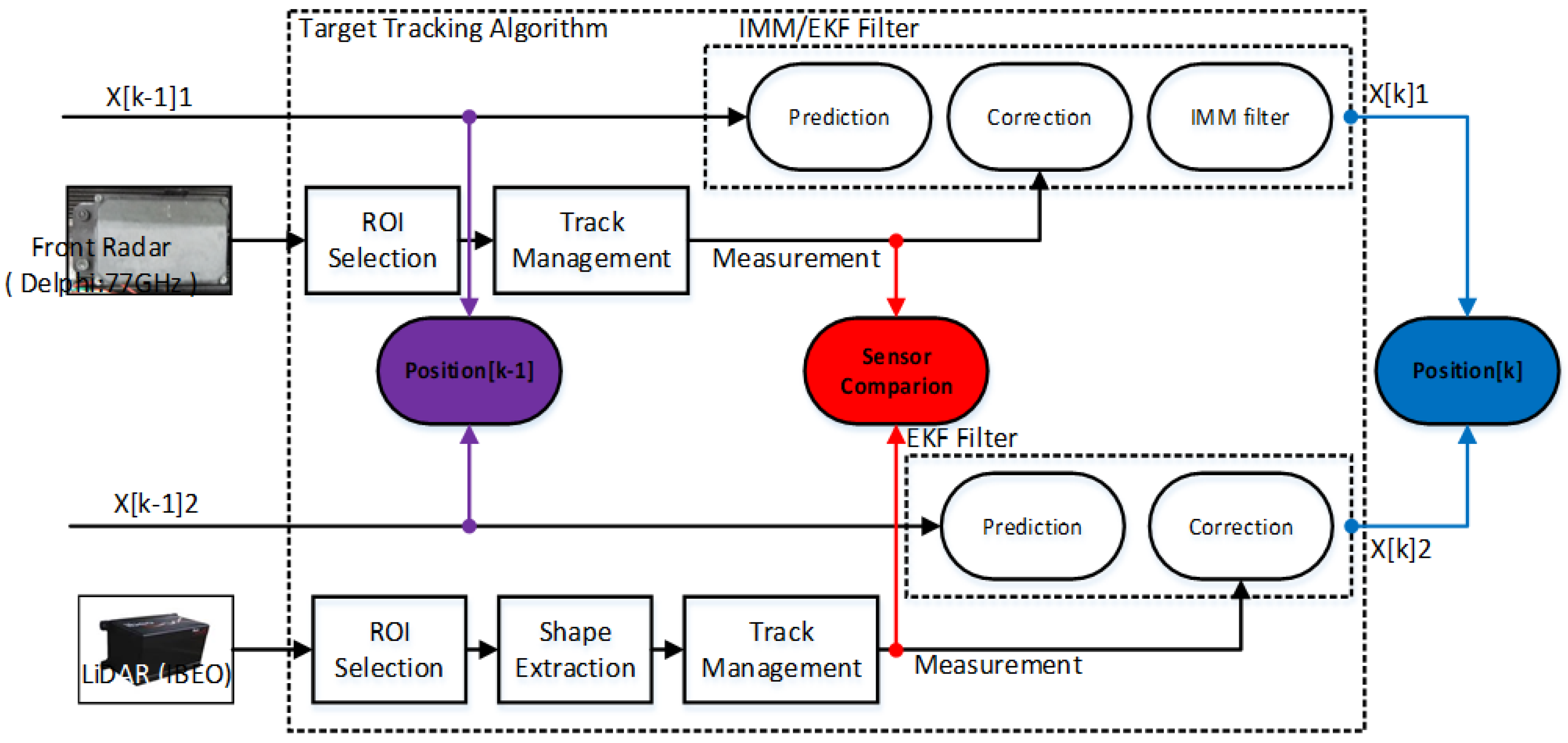
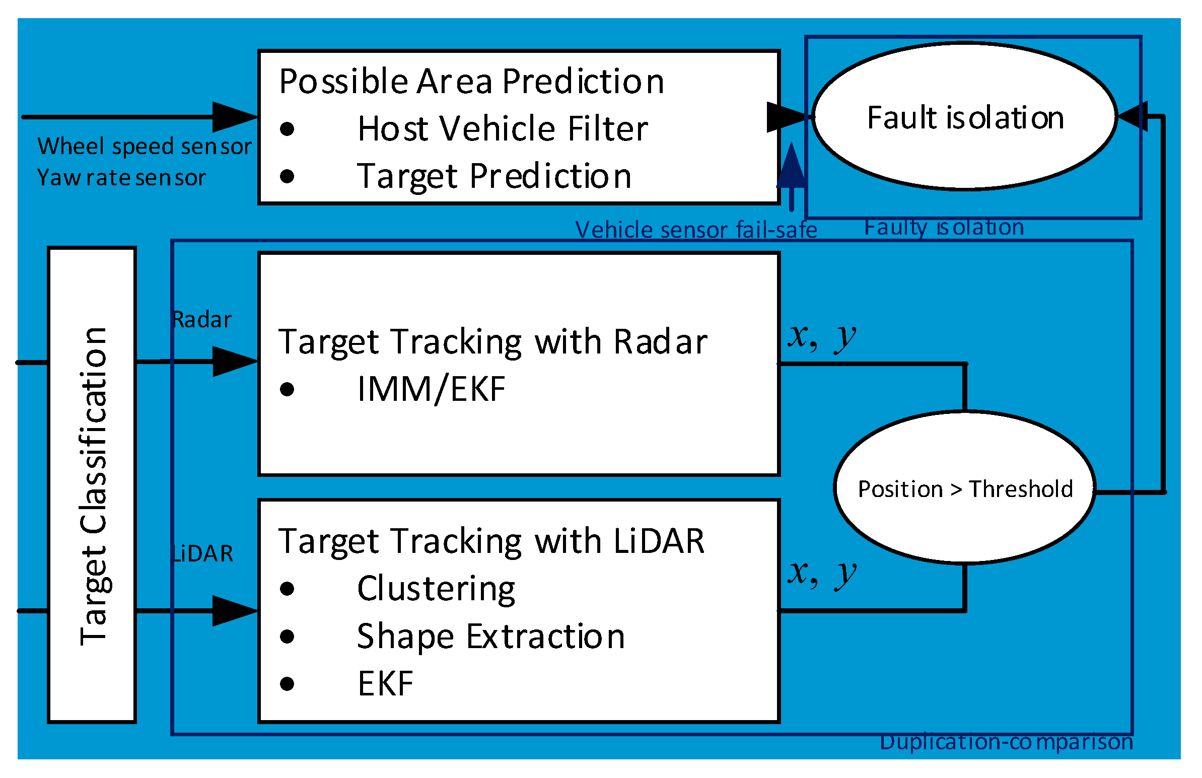
3.5.1. Modified Duplication Comparison

In this part, a modified duplication-comparison method is used. The overall structure of the method is illustrated in Figure 7. The two branches are the tracking algorithms of radar and LiDAR, respectively. In addition, inputs are defined as the estimation previously made and measurements are defined as longitudinal and lateral positions of radar and LiDAR measurements. If the estimated target’s position at the k^th step would be different between two sensors, the algorithm checks whether it is from sensor measurements or inputs. If it is from the inputs, there is no meaning. If it is from the sensor measurements, there should be faults in the sensors themselves. On the other hand, this mechanism can be stated in another way. When the assumption is that there is a real vehicle (if it is validated as a vehicle by both sensors over ten seconds is true), there should be an anomaly in the sensing system when the estimation results deviate from each other.

3.5.2. Fault Isolation

In Bader’s work [9], location of the fault was identified by comparing residuals from each branch. However, it is hard to isolate faults with a target-tracking filter because not only is it more complicated but also the filter selects the most relevant measurements based on the residual—i.e., the measurement that has low residual is selected in the track management phase. Therefore, faults are identified by using possible area in this paper. As illustrated in Figure 8, if the sensor’s measurements that are not measured within the possible area, the sensor is identified as a faulty sensor.

3.6. In-Vehicle Sensor Fail-Safes

Since the wheel speed sensors and yaw rate sensor are used in this algorithm, their faulty behavior should also be detected. To assure the functional safety of in-vehicle sensors, the concept of hypothesis testing is used.

The predicted future estimations of surrounding vehicles are stuck at every iteration. Originally, they are almost the same since they estimate the same vehicle at specific time. However, because they are rotated and transferred every step as the host vehicle moves, the last estimations would be far different from the others when one of those sensors malfunctions. Therefore, the assumption is that the standard deviation of the saved estimations is small only when the in-vehicle sensors function normally.

3.7. Online Update

The suggested algorithm that ran every iteration after the existence of surrounding vehicles in real-time is validated. It saves the target predictions for every 1 s. The overall flow of algorithm is described as follows.

Algorithm 1 Online algorithm of exteroceptive sensor fail-safe

$\begin{array}{l}for \mathrm{Each} \mathrm{target} \mathrm{number}(1~8)\\ if \mathrm{Confidence} \mathrm{of} \mathrm{the} \mathrm{target} \mathrm{estimated} \mathrm{by} \mathrm{both} \mathrm{sensors} > 100 \& \\ \mathrm{Dis} < \mathrm{Y}\\ \mathrm{Fail}-\mathrm{safe} \mathrm{trigger} \mathrm{ON};\\ \mathrm{Target} \mathrm{prediction} \& \mathrm{Save};\\ elseif \mathrm{Fail}-\mathrm{safe} \mathrm{trigger} \mathrm{ON} \& \mathrm{Dis} < \mathrm{Y}\\ \mathrm{Target} \mathrm{prediction} \& \mathrm{Save};\\ elseif \mathrm{Fail}-\mathrm{safe} \mathrm{trigger} \mathrm{ON} \& \mathrm{Dis} < \mathrm{Y}\\ \mathrm{Do} \mathrm{not} \mathrm{predict} \mathrm{the} \mathrm{target};\\ elseif \mathrm{Fail}-\mathrm{safe} \mathrm{trigger} \mathrm{ON} \& \\ \mathrm{Confidence} \mathrm{of} \mathrm{the} \mathrm{target} \mathrm{estimated} \mathrm{by} \mathrm{both} \mathrm{sensors} < 10\\ \mathrm{Fail}-\mathrm{safe} \mathrm{trigger} \mathrm{OFF};\\ \mathrm{Stop} \mathrm{the} \mathrm{fail}-\mathrm{safe} \mathrm{algorithm};\\ else\\ end\\ if \mathrm{Fail}-\mathrm{safe} \mathrm{trigger} \mathrm{ON} \& \mathrm{Dis}\left[\mathrm{k}\right] > \mathrm{Y} \& \mathrm{Dis}[\mathrm{k}-1] < \mathrm{Y}\\ \mathrm{Fault} \mathrm{isolation};\\ elseif \mathrm{Fail}-\mathrm{safe} \mathrm{trigger} \mathrm{ON}\\ \mathrm{Vehicle} \mathrm{sensor} \mathrm{fail}-\mathrm{safe};\\ else\\ end\\ end\\ \mathrm{where}, \mathrm{Dis} = \mathrm{distance} \mathrm{between} \mathrm{the} \mathrm{etimations} \\ \mathrm{Y} = \mathrm{lane} \mathrm{width}\end{array}$

4. Fault Injection Experiment with Real-Driving Data

To verify the proposed algorithm, the offline simulation-based fault injection experiment was conducted via MATLAB. This section describes the details of the real-driving data and the fault injection experiment.

4.1. Description of Real-Driving Data

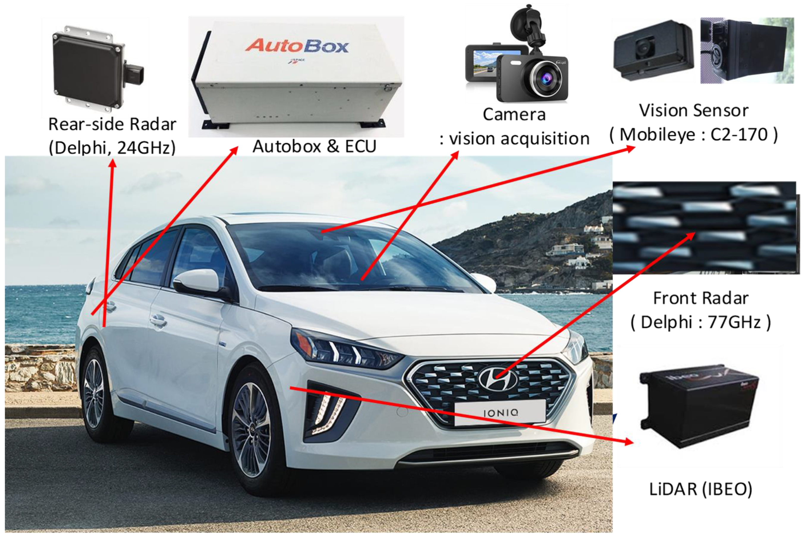
The real-driving data used for fault injection experiments were recorded when the test vehicle was driven on the urban road of Changwon-Si in Korea. The test vehicle is described in Figure 9. It is a sedan equipped with various in-vehicle sensors, a camera, a vision sensor, radars and a LiDAR. The radar installed in the vehicle is a Delphi radar with 77 GHz. In addition, LiDAR installed in the vehicle is an IBEO LiDAR. It is an about 1.1 km of the urban road of Changwon-Si which includes significant road curvature. The aforementioned sensors sensed not only the preceding vehicle but also various environmental factors, such as parked cars, curbs, trees or fences, during driving.

One of the most important parts of autonomous driving technology is perception. In order for a car to drive by itself, it is essential to know where it is and what there is around it. Therefore, various sensors have been used for automated cars as described in Figure 10. Sensors were classified according to their usage.

4.2. Experiment Results

Simulation-based fault injection was conducted with real-driving data via MATLAB. Additive faults were injected into sensor systems of the autonomous driving system that was introduced in Section 2. The injected faults assumed that the significant noise added to sensor’s range or angle signals or that some offsets occurred in the sensor system. As can be seen in

Table 1. Results of fault injection experiments.

Location	Type	${\mathit{t}}_{\mathit{D}}$
		Error	Sensor Fault	Isolation
Radar sensor Range	+10 m additive fault	1.4 s	1.4 s	1.4 s
	+10 m additive noise	3.8 s	3.8 s	3.8 s
Radar sensor Angle	+10 degree additive fault	2.2 s	2.2 s	2.2 s
	+10 degree additive noise	X	X	X
	+15 degree additive fault	1.0 s	1.0 s	1.0 s
Laser scanner Range	+10 m additive fault	1.4 s	1.4 s	1.4 s
	+10 m additive noise	1.4 s	1.4 s	X
Laser scanner Angle	+10 degree additive fault	1.1 s	1.1 s	1.1 s
	+10 degree additive noise	1.2 s	1.2 s	1.2 s
	+15 degree additive fault	1.0 s	1.0 s	1.0 s

, most faults were detected in a relatively short time—three seconds—and were well-detected. However, in the case that the small angle deviation on radar sensor occurs, neither the proposed algorithm detects the fault nor does a hazardous situation occur.

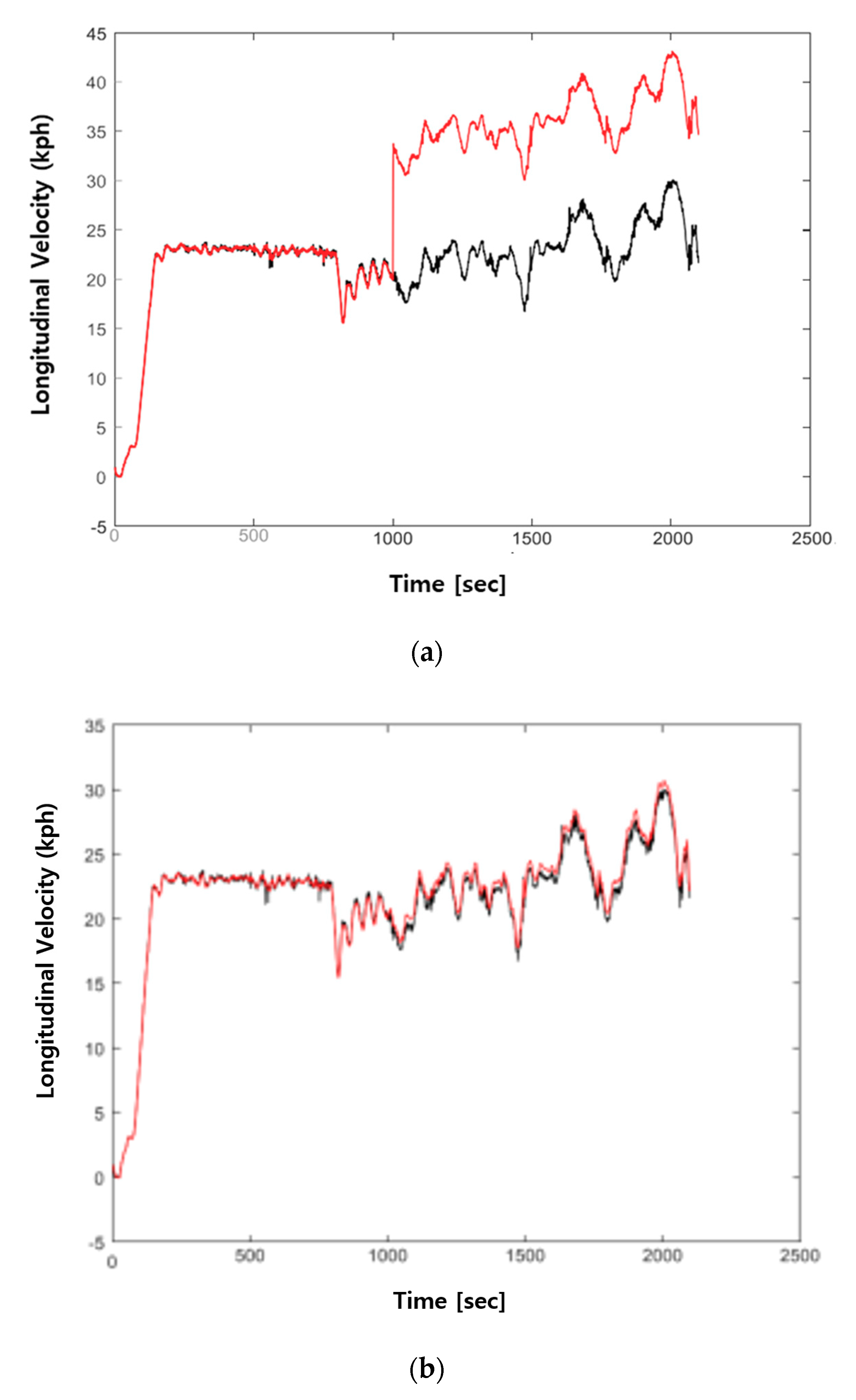
The estimated velocity of the host vehicle and the driving data are plotted in Figure 11a. The black solid line indicates vehicle velocity without faults in sensors and the red solid line indicates vehicle velocity when the rear-right wheel speed sensor failed. The 7.5 m/s additive fault was injected into the simulation at 100 s. When the Kalman filter equips the fail-safe algorithm, there is no difference between the estimated velocity without faults and that with faults as described in Figure 11b.

5. Conclusions

External sensors, such as a camera, an automotive radar or a LiDAR, have played an important role in sensing and perception for autonomous vehicles. Thus, along with the development of a high-level automated driving system, achieving these sensors’ robustness becomes gradually more important. In this paper, to assure the robust situation awareness, a fail-safe algorithm for an exteroceptive sensor of autonomous vehicle has been proposed. A modified duplication-comparison method is used for the algorithm. A novelty of this work lies on the fault isolation mechanism, which diagnoses a faulty sensor with predictions of the target estimations.

To verify the proposed algorithm, the offline simulation-based fault injection experiment was conducted via MATLAB. Various types of additive faults are designed and injected into the autonomous driving system introduced in Section 2. The results of the experiments are also presented.

In the future, our ultimate goal is to achieve a higher reliability by designing an entire fail-safe algorithm, which assures not only a robust situation awareness but also the safety of the autonomous driving system.

Extension of the test target to a more complex and realistic autonomous driving system in order to predict the accurate effects of radar sensor failure on autonomous driving systems is the topic of our future research. Comparison of the algorithm currently functioning in vehicles with the proposed algorithm is another topic of our future works.

References

- Englund, C.; Estrada, J.; Jaaskelainen, J.; Misener, J.; Satyavolu, S.; Serna, F.; Sundararajan, S. Enabling Technologies for Road Vehicle Automation. In Road Vehicle Automation 4; Springer: Berlin/Heidelberg, Germany, 2018; pp. 177–185. [Google Scholar]
- Sundvall, P.; Jensfelt, P. Fault Detection for Mobile Robots Using Redundant Positioning Systems. In 2006 IEEE International Conference on Robotics and Automation; ICRA 2006; IEEE: New York, NY, USA, 2006; pp. 3781–3786. [Google Scholar]
- Schmitz, N.; Koch, J.; Proetzsch, M.; Berns, K. Fault-Tolerant 3D Localization for Outdoor Vehicles. In Proceedings of the 2006 IEEE/RSJ International Conference on Intelligent Robots and Systems, Beijing, China, 9–15 October 2006; IEEE: New York, NY, USA, 2006; pp. 941–946. [Google Scholar]
- Blanke, M. Consistent Design of Dependable Control Systems. Control Eng. Pract. 1996, 4, 1305–1312. [Google Scholar] [CrossRef]
- Isermann, R. Fault-Diagnosis Systems: An Introduction from Fault Detection to Fault Tolerance; Springer Science & Business Media: New York, NY, USA, 2006. [Google Scholar]
- Blanke, M.; Kinnaert, M.; Lunze, J.; Staroswiecki, M.; Schröder, J. Diagnosis and Fault-Tolerant Control; Springer: New York, NY, USA, 2006; Volume 2. [Google Scholar]
- Aouaouda, S.; Chadli, M.; Boukhnifer, M. Speed Sensor Fault Tolerant Controller Design for Induction Motor Drive in EV. Neurocomputing 2016, 214, 32–43. [Google Scholar] [CrossRef]
- Chibani, A.; Chadli, M.; Ding, S.X.; Braiek, N.B. Design of Robust Fuzzy Fault Detection Filter for Polynomial Fuzzy Systems with New Finite Frequency Specifications. Automatica 2018, 93, 42–54. [Google Scholar] [CrossRef]
- Benso, A.; Prinetto, P. Fault Injection Techniques and Tools for Embedded Systems Reliability Evaluation; Springer Science & Business Media: New York, NY, USA, 2003; Volume 23. [Google Scholar]
- Arlat, J.; Costes, A.; Crouzet, Y.; Laprie, J.-C.; Powell, D. Fault Injection and Dependability Evaluation of Fault-Tolerant Systems. IEEE Trans. Comput. 1993, 42, 913–923. [Google Scholar] [CrossRef]
- Zug, S.; Kaiserua, J. An Approach towards Smart Fault-Tolerant Sensors. In Proceedings of the 2009 IEEE International Workshop on Robotic and Sensors Environments, Lecco, Italy, 6–7 November 2009; IEEE: New York, NY, USA, 2009; pp. 35–40. [Google Scholar]
- Ricquebourg, V.; Delafosse, M.; Delahoche, L.; Marhic, B.; Jolly-Desodt, A.; Menga, D. Fault Detection by Combining Redundant Sensors: A Conflict Approach within the Tbm Framework. Cogn. Syst. Interact. Sens. COGIS 2007. [Google Scholar]
- Bader, K.; Lussier, B.; Schön, W. A Fault Tolerant Architecture for Data Fusion: A Real Application of Kalman Filters for Mobile Robot Localization. Robot. Auton. Syst. 2017, 88, 11–23. [Google Scholar] [CrossRef]
- Kim, B.; Yi, K.; Yoo, H.-J.; Chong, H.-J.; Ko, B. An IMM/EKF Approach for Enhanced Multitarget State Estimation for Application to Integrated Risk Management System. IEEE Trans. Veh. Technol. 2015, 64, 876–889. [Google Scholar] [CrossRef]
- Wang, D.Z.; Posner, I.; Newman, P. What Could Move? Finding Cars, Pedestrians and Bicyclists in 3d Laser Data. In 2012 IEEE International Conference on Robotics and Automation; IEEE: New York, NY, USA, 2012; pp. 4038–4044. [Google Scholar]
- Kaempchen, N.; Fuerstenberg, K.C.; Skibicki, A.G.; Dietmayer, K.C. Sensor Fusion for Multiple Automotive Active Safety and Comfort Applications. In Advanced Microsystems for Automotive Applications 2004; Springer: Berlin/Heidelberg, Germany, 2004; pp. 137–163. [Google Scholar]
- Dahmani, H.; Chadli, M.; Rabhi, A.; El Hajjaji, A. Vehicle Dynamics and Road Curvature Estimation for Lane Departure Warning System Using Robust Fuzzy Observers: Experimental Validation. Veh. Syst. Dyn. 2015, 53, 1135–1149. [Google Scholar] [CrossRef]
- Shin, D.; Kim, B.; Yi, K. Probabilistic Threat Assessment of Vehicle States Using Wireless Communications for Application to Integrated Risk Management System. In Proceedings of the FAST-zero’15: 3rd International Symposium on Future Active Safety Technology Toward zero traffic accidents, Göteborg, Sweden, 9–11 September 2015. [Google Scholar]
- Wang, R.; Jing, H.; Wang, J.; Chadli, M.; Chen, N. Robust Output-Feedback Based Vehicle Lateral Motion Control Considering Network-Induced Delay and Tire Force Saturation. Neurocomputing 2016, 214, 409–419. [Google Scholar] [CrossRef]
- Shin, D.; Kim, B.; Yi, K.; Carvalho, A.; Borrelli, F. Human-Centered Risk Assessment of an Automated Vehicle Using Vehicular Wireless Communication. IEEE Trans. Intell. Transp. Syst. 2018, 20, 667–681. [Google Scholar] [CrossRef]