Deep Learning-Based Localization for UWB Systems


Abstract
1. Introduction
1.1. Related Work for UWB System Localization
1.2. Our Contribution
- The ranging and positioning phases are integrated, so that error propagation from ranging to positioning can be reduced.
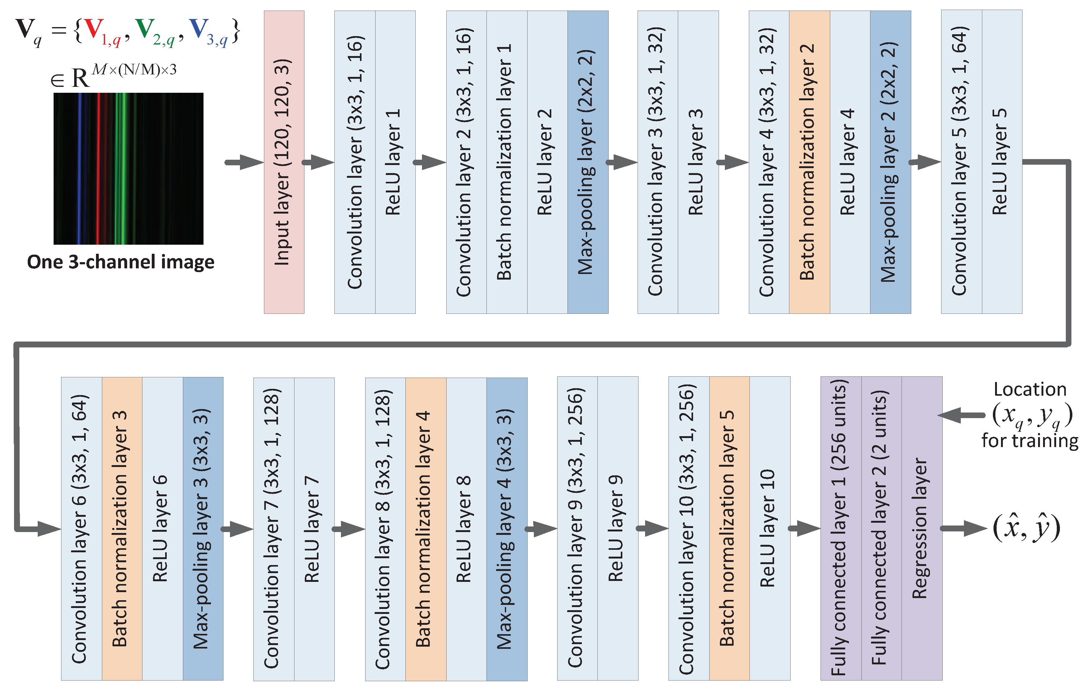
- For the proposed localization method that integrates the ranging and positioning phase, a novel CNN structure is designed, which is trained through three 2D images.
- Compared to the conventional CNN-based localization method in [14] that requires three CNNs, only one CNN is required for the proposed method.
- The proposed method improves localization accuracy with robustness against the asymmetry of the area where the localization is performed.
2. System and Signal Models
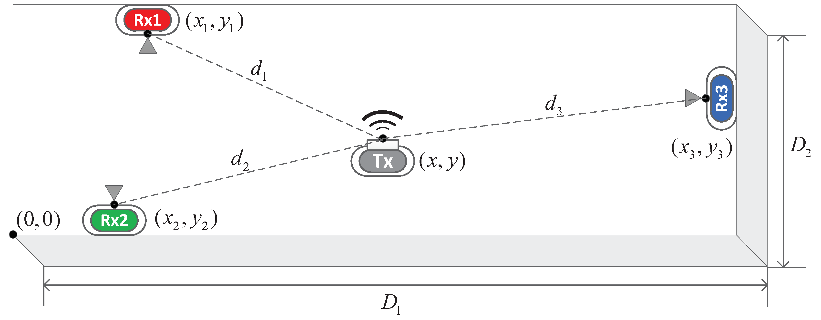
2.1. Localization System Model
- (i)
- Ranging phase: Selected measurements are performed to estimate the distance between transceivers.
- (ii)
- Positioning phase: The measurements are then processed to determine the position of the target.
2.2. Signal and Channel Models
3. Conventional and Proposed Localization Methods
3.1. Conventional ToA-Based Localization Method
3.2. Conventional CNN-DE Method
3.3. Proposed CNN-LE Method
4. Simulation Results
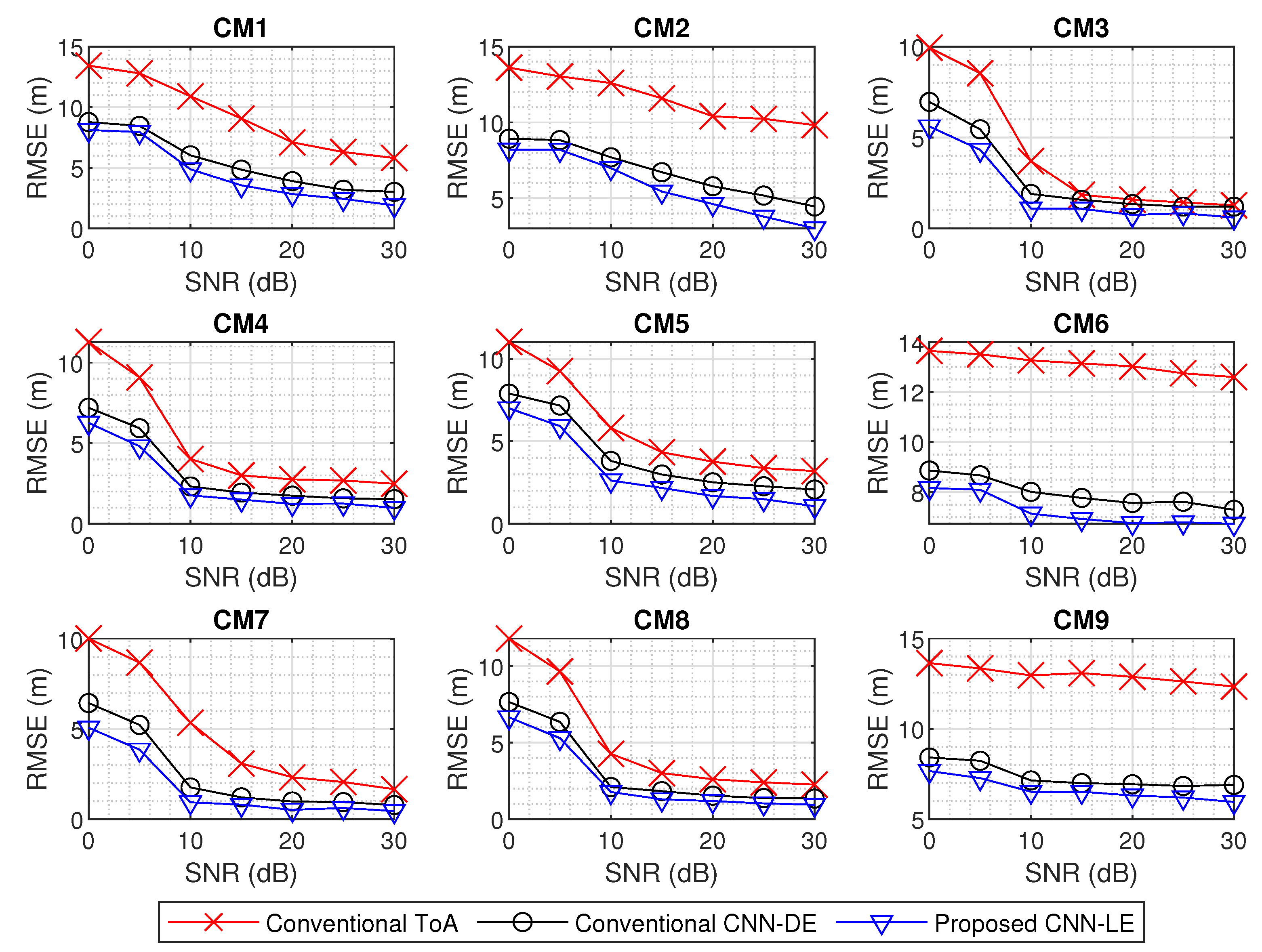
4.1. Performance with Respect to SNR
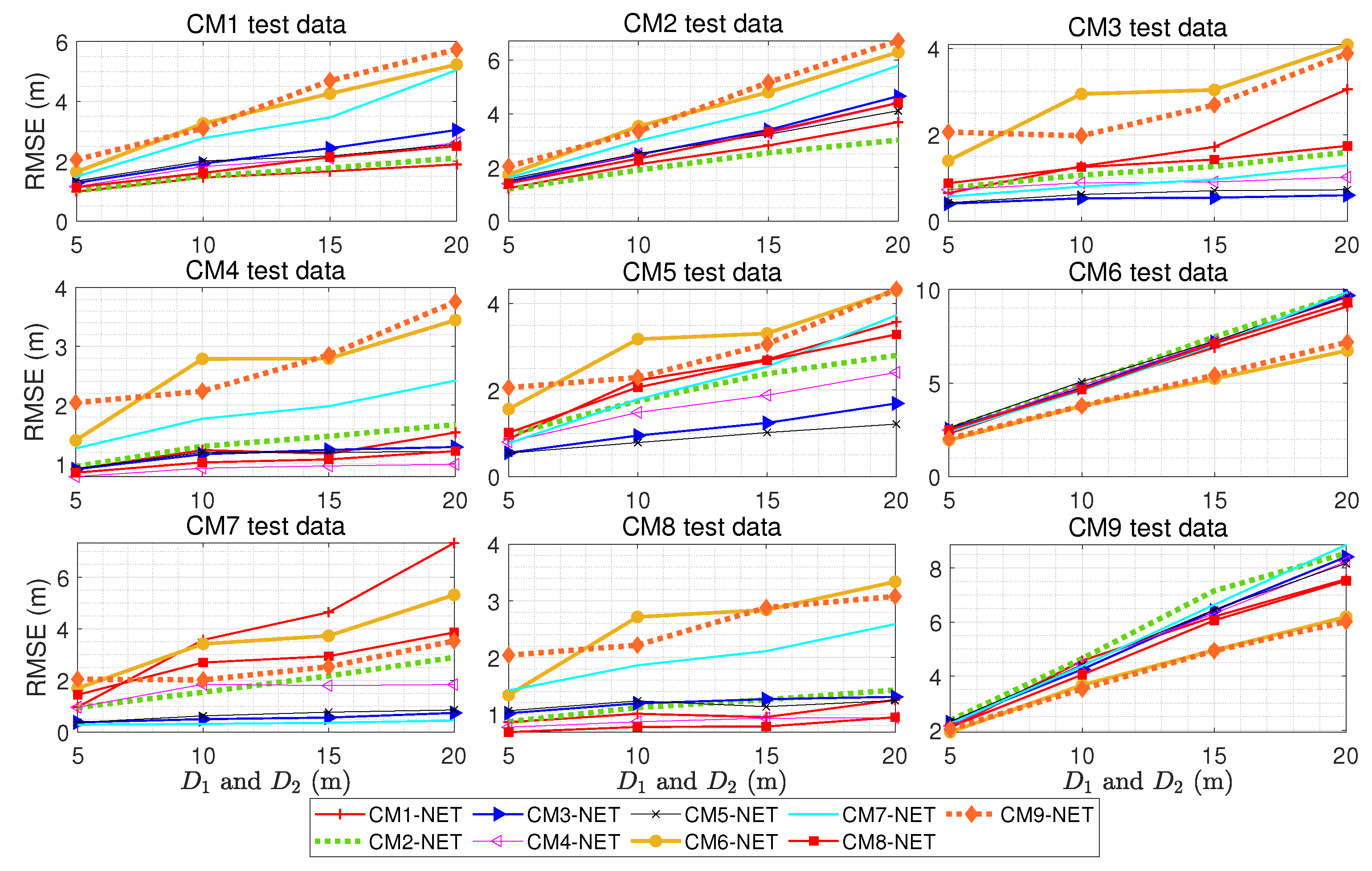
4.2. Performance with Respect to Map Size
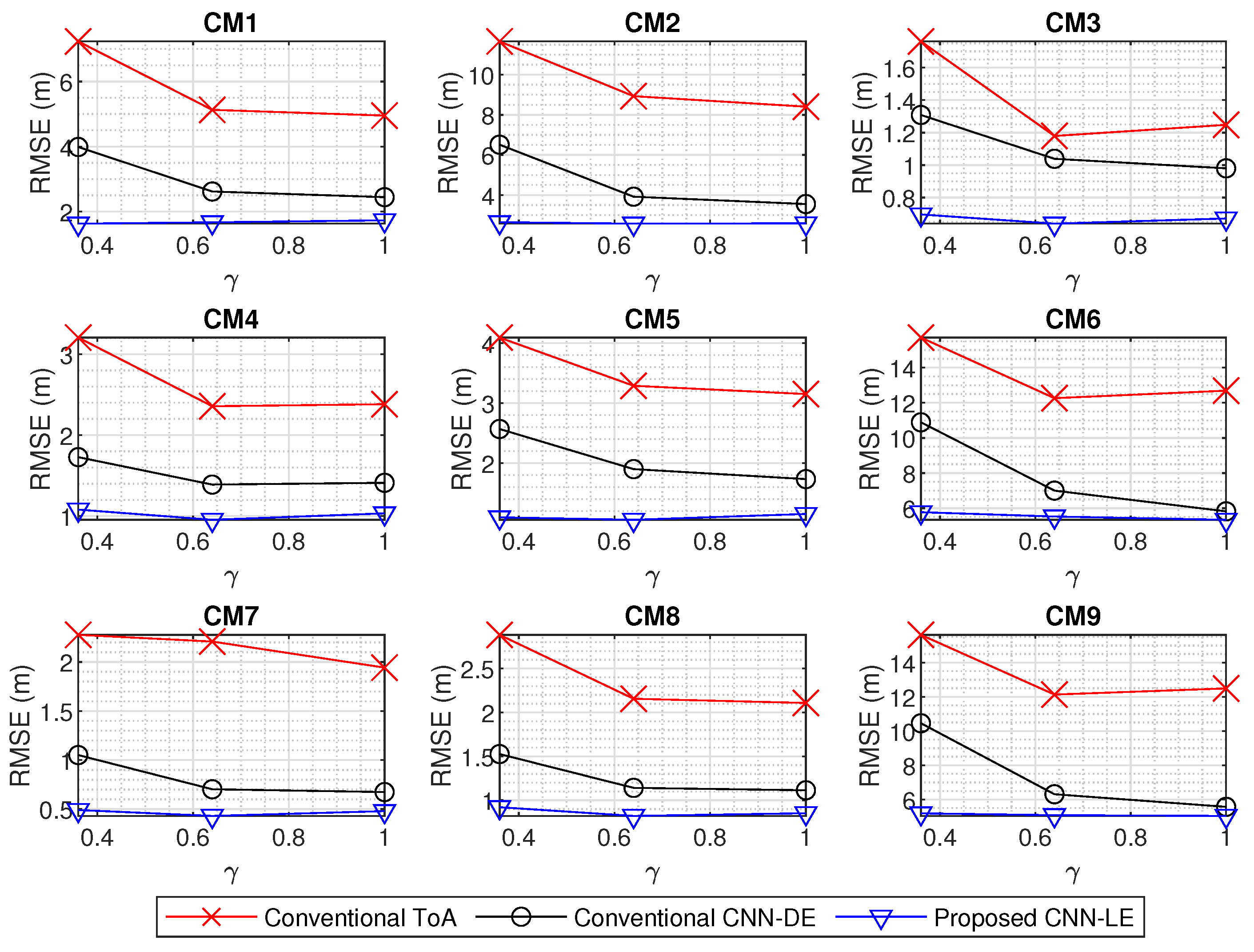
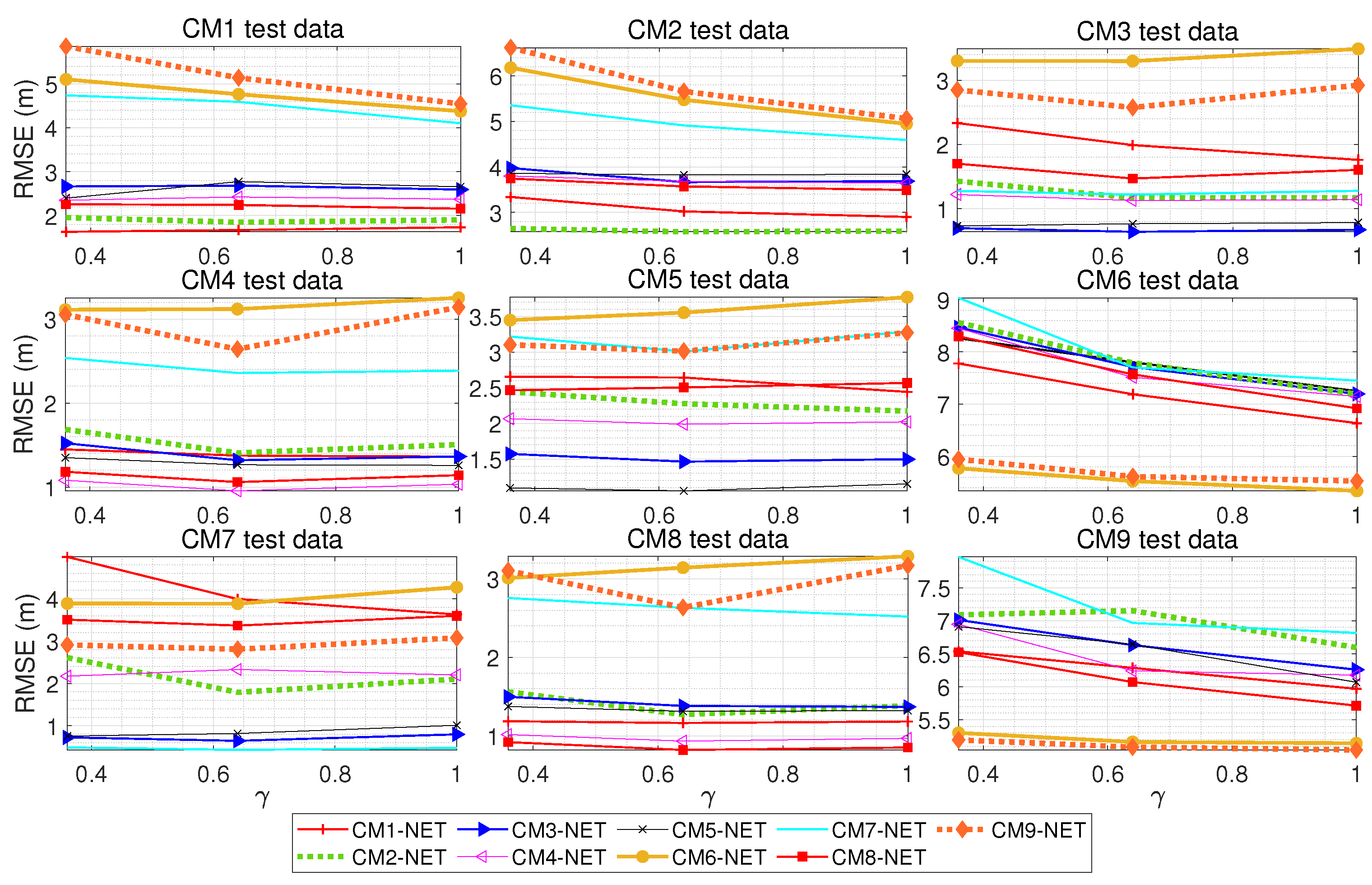
4.3. Performance with Respect to Asymmetry of the Area
5. Conclusions
Author Contributions
Funding
Conflicts of Interest
Abbreviations
| AoA | Angle-of-Arrival |
| CIR | Channel Impulse Response |
| CM | Channel Model |
| CM-NET | Channel Model Network |
| CNN | Convolutional Neural Network |
| CNN-DE | Convolutional Neural Network-based Distance Estimation |
| CNN-LE | Convolutional Neural Network-based Location Estimation |
| CSI | Channel State Information |
| DNN | Deep Neural Network |
| LoS | Line-of-Sight |
| LSTM | Long-Short-Term-Memory |
| MPC | Multi-Path Components |
| NLoS | Non-Line-of-Sight |
| PDP | Power Delay Profiles |
| ReLU | Rectified Linear Unit |
| RFID | Radio Frequency Identification Device |
| RGB | Red-Green-Blue |
| RMSE | Root Mean Squared Error |
| RNN | Recurrent Neural Network |
| RSS | Received Signal Strength |
| SGDM | Stochastic Gradient Descent with Momentum |
| SNR | Signal-to-Noise Ratio |
| ToA | Time-of-Arrival |
| UWB | Ultra Wideband |
| Wi-Fi | Wireless Fidelity |
References
- Zafari, F.; Gkelias, A.; Leung, K.K. A Survey of Indoor Localization Systems and Technologies. IEEE Commun. Surv. Tutor. 2019, 21, 2568–2599. [Google Scholar] [CrossRef]
- Taponecco, L.; D’Amico, A.A.; Mengali, U. Joint TOA and AOA Estimation for UWB Localization Applications. IEEE Trans. Wirel. Commun. 2011, 10, 2207–2217. [Google Scholar] [CrossRef]
- Yu, K.; Wen, K.; Li, Y.; Zhang, S.; Zhang, K. A Novel NLOS Mitigation Algorithm for UWB Localization in Harsh Indoor Environment. IEEE Trans. Veh. Technol. 2019, 68, 686–699. [Google Scholar] [CrossRef]
- Zwirello, L.; Schipper, T.; Harter, M.; Zwick, T. UWB Localization System for Indoor Applications: Concept, Realization and Analysis. J. Electr. Comput. Eng. 2012, 2012, 849638. [Google Scholar] [CrossRef]
- Rana, S.P.; Dey, M.; Siddiqui, H.U.; Tiberi, G.; Ghavami, M.; Dudley, S. UWB localization employing supervised learning method. In Proceedings of the IEEE International Conference on Ubiquitous Wireless Broadband (ICUWB), Salamanca, Spain, 12–15 September 2017; pp. 1–5. [Google Scholar]
- Hsieh, C.-H.; Chen, J.-Y.; Nien, B.-H. Deep Learning-Based Indoor Localization Using Received Signal Strength and Channel State Information. IEEE Access 2019, 7, 33256–33267. [Google Scholar] [CrossRef]
- Khatab, Z.E.; Hajihoseini, A.; Ghorashi, S.A. A Fingerprint Method for Indoor Localization Using Autoencoder Based Deep Extreme Learning Machine. IEEE Sens. Lett. 2018, 2, 1–4. [Google Scholar] [CrossRef]
- Sinha, R.S.; Hwang, S.-H. Comparison of CNN Applications for RSSI-Based Fingerprint Indoor Localization. Electronics 2019, 8, 989. [Google Scholar] [CrossRef]
- Flix, G.; Siller, M.; lvarez, E.N. A fingerprinting indoor localization algorithm based deep learning. In Proceedings of the International Conference on Ubiquitous and Future Networks (ICUFN), Vienna, Austria, 5–8 July 2016; pp. 1006–1011. [Google Scholar]
- Chen, Z.; Zou, H.; Yang, J.; Jiang, H.; Xie, L. WiFi Fingerprinting Indoor Localization Using Local Feature-Based Deep LSTM. IEEE Syst. J. 2019, 14, 3001–3010. [Google Scholar] [CrossRef]
- Hoang, M.T.; Yuen, B.; Dong, X.; Lu, T.; Westendorp, R.; Reddy, K. Recurrent Neural Networks for Accurate RSSI Indoor Localization. IEEE Internet Things J. 2019, 6, 10639–10651. [Google Scholar] [CrossRef]
- Zhang, Y.; Qu, C.; Wang, Y. An Indoor Positioning Method Based on CSI by Using Features Optimization Mechanism with LSTM. IEEE Sens. J. 2020, 20, 4868–4878. [Google Scholar] [CrossRef]
- Wang, X.; Wang, X.; Mao, S. Deep Convolutional Neural Networks for Indoor Localization with CSI Images. IEEE Trans. Netw. Sci. Eng. 2018, 7, 316–327. [Google Scholar] [CrossRef]
- Joung, J.; Jung, S.; Chung, S.; Jeong, E.-R. CNN-Based Tx–Rx Distance Estimation for UWB System Localisation. Electr. Lett. 2019, 55, 938–940. [Google Scholar] [CrossRef]
- Sayed, A.H.; Tarighat, A.; Khajehnouri, N. Network-Based Wireless Location: Challenges Faced in Developing Techniques for Accurate Wireless Location Information. IEEE Signal Process. Mag. 2005, 22, 24–40. [Google Scholar] [CrossRef]
- Poulose, A.; Han, D.S. UWB Indoor Localization Using Deep Learning LSTM Networks. Appl. Sci. 2020, 10, 6290. [Google Scholar] [CrossRef]
- Dardari, D.; Conti, A.; Ferner, U.; Giorgetti, A.; Win, M.Z. Ranging with Ultrawide Bandwidth Signals in Multipath Environments. IEEE Proc. 2009, 97, 404–426. [Google Scholar] [CrossRef]
- Guvenc, I.; Sahinoglu, Z. Threshold-based TOA estimation for impulse radio UWB systems. In Proceedings of the International Conference on Ultra-Wideband (ICUWB), Zurich, Switzerland, 5–8 September 2005; pp. 420–425. [Google Scholar]
- Molisch, A.F. Ultrawideband Propagation Channels-Theory, Measurement, and Modeling. IEEE Trans. Veh. Technol. 2005, 54, 1528–1545. [Google Scholar] [CrossRef]
- Guvenc, I.; Sinan, G.; Sahinoglu, Z. Fundamental Limits and Improved Algorithms for Linear Least-Squares Wireless Position Estimation. Wirel. Commun. Mob. Comput. 2012, 12, 1037–1052. [Google Scholar] [CrossRef]
- Cassioli, D.; Win, M.Z.; Molisch, A.F. The Ultra-Wide Bandwidth Indoor Channel From Statistical Model to Simulations. IEEE J. Sel. Areas Commun. 2002, 20, 1247–1257. [Google Scholar] [CrossRef]
- Molisch, A.F.; Balakrishnan, K.; Cassioli, D.; Chong, C.-C.; Emami, S.; Fort, A.; Karedal, J.; Kunisch, J.; Schantz, H.; Schuster, U.; et al. IEEE 802.15.4a Channel Model-Final Report; Tech. Rep., Doc. IEEE 802.1504-0062-02-004a; IEEE: Piscataway, NJ, USA, 2005. [Google Scholar]
- Turin, G. An introduction to matched filters. IRE Trans. Inf. Theory 1960, 6, 311–329. [Google Scholar] [CrossRef]
- Liu, W.; Ding, H.; Huang, X.; Liu, Z. TOA Estimation in IR UWB Ranging with Energy Detection Receiver Using Received Signal Characteristics. IEEE Commun. Lett. 2012, 16, 738–741. [Google Scholar] [CrossRef]
- Celebi, H.; Guvenc, I.; Arslan, H. On the statistics of channel models for UWB ranging. In Proceedings of the IEEE Sarnoff Symposium, Princeton, NJ, USA, 27–28 March 2006; pp. 1–4. [Google Scholar]
- Create a Regression Output Layer—MATLAB Regression Layer. Available online: https://www.mathworks.com/help/deeplearning/ref/regressionlayer.html (accessed on 28 September 2020).
- Flasi, C.; Dardari, D.; Mucchi, L.; Win, M.Z. Range estimation in UWB realistic environments. In Proceedings of the IEEE International Conference on Communications (ICC), Istanbul, Turkey, 11–15 June 2006; pp. 5692–5697. [Google Scholar]


| Channel Model | Environment |
|---|---|
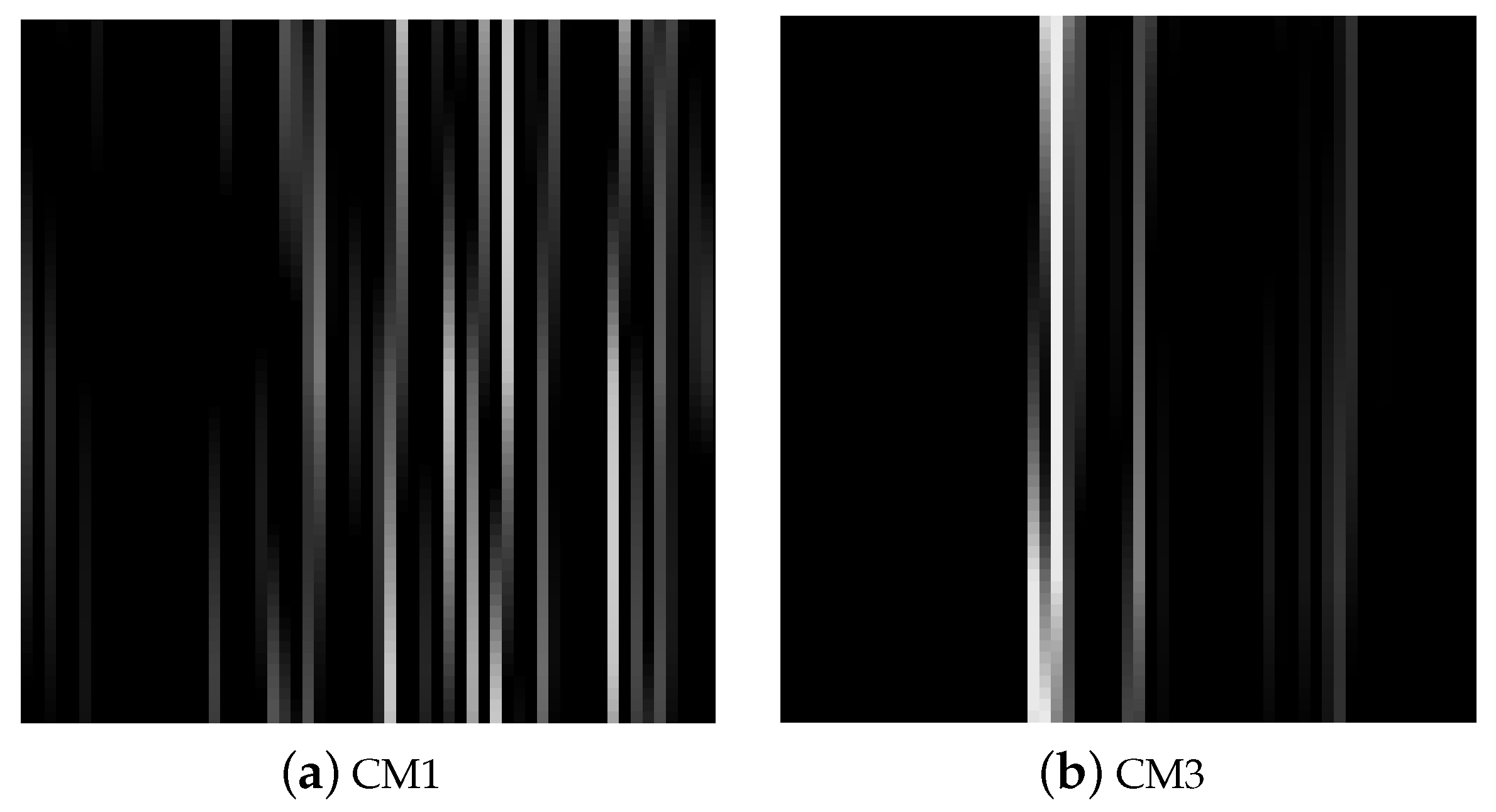
| CM1 | Residential, LoS |
| CM2 | Residential, NLoS |
| CM3 | Office, LoS |
| CM4 | Office, NLoS |
| CM5 | suburban LoS |
| CM6 | suburban NLoS |
| CM7 | Industrial, LoS |
| CM8 | Industrial, NLoS |
| CM9 | Open Outdoor (Snow-covered, farm) |
| Step | Procedure |
|---|---|
| 1 | Collect the received signals , , and in (3) from Rx’s 1, 2, and 3, respectively. |
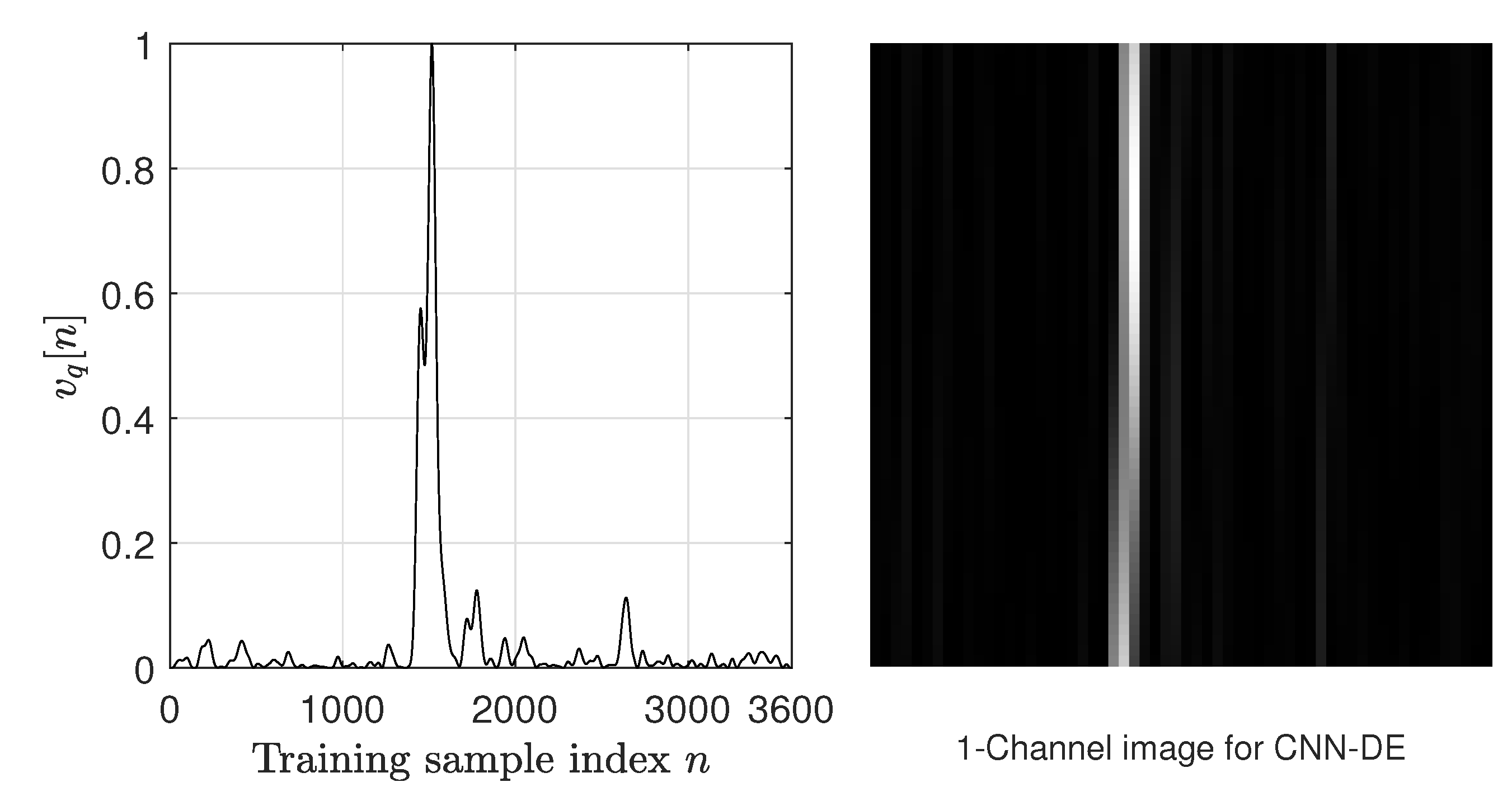
| 2 | Generate the normalized and oversampled absolute sequence of the received signals, i.e., , , and , from (4). |
| 3 | Generate three 2D images, i.e., , , and , from (5). |
| 4 | Generate the input of CNN-LE, i.e., . |
| 5 | Provide to CNN-LE shown in Figure 5. |
| 6 | Obtain the estimation of the location from the CNN-LE output. |
| Parameters | CNN-DE | CNN-LE |
|---|---|---|
| Number of input layers | 1 | 1 |
| Number of convolutional layers | 4 | 10 |
| Number of batchnorm layers | 4 | 5 |
| Number of ReLU layers | 4 | 10 |
| Number of max-pooling layers | 3 | 4 |
| Number of fully connected layers | 1 | 2 |
| Number of regression layers | 1 | 1 |
| Number of total layers | 18 | 33 |
| Options | CNN-DE | CNN-LE |
|---|---|---|
| Solver | SGDM | SGDM |
| Initial learn rate | 0.001 | 0.02 |
| Gradient threshold | infinite | 1 |
| Learn rate drop period | 1 | 2 |
| Learn rate drop factor | 0.9 | 0.9 |
| Shuffle | every epoch | every epoch |
| Max epoch | 30 | 30 |
| Mini batch size | 200 | 200 |
| Validation frequency (iterations) | 50 | 100 |
| Number of epochs to converge | 19 | 29 |
| Training time | 2 min | 16 min |
| Localization time | 2.2 s | 6.1 s |
Publisher’s Note: MDPI stays neutral with regard to jurisdictional claims in published maps and institutional affiliations. |
© 2020 by the authors. Licensee MDPI, Basel, Switzerland. This article is an open access article distributed under the terms and conditions of the Creative Commons Attribution (CC BY) license (http://creativecommons.org/licenses/by/4.0/).
Share and Cite
Nguyen, D.T.A.; Lee, H.-G.; Jeong, E.-R.; Lee, H.L.; Joung, J. Deep Learning-Based Localization for UWB Systems. Electronics 2020, 9, 1712. https://doi.org/10.3390/electronics9101712
Nguyen DTA, Lee H-G, Jeong E-R, Lee HL, Joung J. Deep Learning-Based Localization for UWB Systems. Electronics. 2020; 9(10):1712. https://doi.org/10.3390/electronics9101712
Chicago/Turabian StyleNguyen, Doan Tan Anh, Han-Gyeol Lee, Eui-Rim Jeong, Han Lim Lee, and Jingon Joung. 2020. "Deep Learning-Based Localization for UWB Systems" Electronics 9, no. 10: 1712. https://doi.org/10.3390/electronics9101712
APA StyleNguyen, D. T. A., Lee, H.-G., Jeong, E.-R., Lee, H. L., & Joung, J. (2020). Deep Learning-Based Localization for UWB Systems. Electronics, 9(10), 1712. https://doi.org/10.3390/electronics9101712