Article

Temporal Auditory Coding Features for Causal Speech Enhancement

School of Electrical and Computer Engineering, Faculty of Engineering, Aristotle University of Thessaloniki, 54124 Thessaloniki, Greece
*
Author to whom correspondence should be addressed.
Electronics 2020, 9(10), 1698; https://doi.org/10.3390/electronics9101698
Submission received: 24 September 2020 / Revised: 12 October 2020 / Accepted: 14 October 2020 / Published: 16 October 2020
(This article belongs to the Special Issue Application of Neural Networks in Biosignal Process)

Abstract

:
Perceptually motivated audio signal processing and feature extraction have played a key role in the determination of high-level semantic processes and the development of emerging systems and applications, such as mobile phone telecommunication and hearing aids. In the era of deep learning, speech enhancement methods based on neural networks have seen great success, mainly operating on the log-power spectra. Although these approaches surpass the need for exhaustive feature extraction and selection, it is still unclear whether they target the important sound characteristics related to speech perception. In this study, we propose a novel set of auditory-motivated features for single-channel speech enhancement by fusing temporal envelope and temporal fine structure information in the context of vocoder-like processing. A causal gated recurrent unit (GRU) neural network is employed to recover the low-frequency amplitude modulations of speech. Experimental results indicate that the exploited system achieves considerable gains for normal-hearing and hearing-impaired listeners, in terms of objective intelligibility and quality metrics. The proposed auditory-motivated feature set achieved better objective intelligibility results compared to the conventional log-magnitude spectrogram features, while mixed results were observed for simulated listeners with hearing loss. Finally, we demonstrate that the proposed analysis/synthesis framework provides satisfactory reconstruction accuracy of speech signals.

1. Introduction

Single-channel speech enhancement has attracted considerable research attention for years due to the emerging demand in various real-world applications, such as mobile phone telecommunication [1,2], automatic speech recognition [3], speech coding [4], and hearing aids [5]. The goal of speech enhancement is to improve the intelligibility and quality of degraded speech signals by suppressing the noise components that impede communication and proper analysis. These include interfering sounds, noise, reverberation, distortion, and other deficiencies [6]. One major challenge for speech enhancement systems is the ability to operate online. Real-time applications of speech enhancement, such as mobile telecommunication and hearing aids, usually cannot afford to access future observations, in favor of low-latency inference. Thus, the requisite for causal processing is apparent in real-world practice.
Numerous speech enhancement algorithms have been established in recent decades. Techniques such as spectral subtraction [7,8] and various forms of Wiener filtering [1,9] have been widely used in speech enhancement frameworks. With the surge of deep learning, supervised learning methods based on neural networks have shown promising performance in a variety of audio applications [10,11,12,13,14,15], including single-channel speech enhancement [5,16,17]. Current state-of-the-art methods exploit large amounts of training data captured under various noise and reverberation conditions [18] and can achieve high generalization performance, even in challenging acoustic environments [19]. Prevailing approaches are based on alternative types of neural networks, such as convolutional and recurrent neural networks, to formulate speech enhancement as a sequence-to-sequence mapping that leverages spectral and temporal correlations while reducing translational variance in signals [6].
Recently, Lang and Yang (2020) [20] demonstrated the effectiveness of fusing complementary features to magnitude-aware targets by separately learning phase representations. In addition, Bae et al. (2019) [21] explored a framework for disentangling speech and noise for noise-invariant speech enhancement, offering more robust noise-invariant properties. In Rao and Carney (2014) [22], a vowel enhancement strategy is proposed to restore the representation of formants at the level of the midbrain by performing formant tracking and enhancement. Causal methods that operate directly on the time domain have also been proposed for speech enhancement and text-to-speech tasks [23], although are of much greater complexity than conventional spectral masking approaches. Even though the time-frequency domain appears more convenient for exploiting the spectro-temporal structure of sound, time-domain methods recently demonstrated impressive results that minimize audible artifacts either by processing raw audio waveforms or temporal audio features, such as the temporal envelope of noise-corrupted signals [24].
While the analysis of speech sounds in mainstream audio applications emphasizes on the frequency spectrum, rate-place encoding on its own fails to account for the majority of perceptual aspects of complex sounds [25]. Nevertheless, a great interest in purely temporal properties of speech has emerged recently, due to their capability in determining the corresponding perceptual attributes. The temporal structure of speech is classified into three categories of speech cues based on dominant temporal fluctuation rates, according to [26]. They are envelope, periodicity, and fine structure cues. In this scheme, envelope cues contain modulation frequencies from 2 to 50 Hz, representing acoustical aspects of phonetic segments combined with stress and voicing information. Periodicity cues exist from 50 to 500 Hz and transmit information about voicing and intonation. Periodicities of higher frequencies, from 0.6 to 10 kHz, comprise the fine structure of the speech signal and convey information related to aspects of consonant place and vowel quality.
In recent years, a wealth of studies conducted with normal-hearing and hearing-impaired listeners showed that accurate speech identification can be obtained by preserving the low-frequency amplitude modulations, primarily the temporal envelope, even if speech is severely degraded in the spectral domain [26,27,28]. On the other hand, individuals with normal hearing show a great ability for understanding speech, even in adverse listening environments, where the acuity of envelope cues is not preserved. This requires the utilization of fine structure cues, in order to effectively facilitate modulation detection [29] and release from masking [30] processes.
To account for this ability in hearing loss, several studies have attempted to recover the temporal structure of speech from noisy environments [31,32,33], while others concentrated on the effects of auditory masking and vocoding on speech perception [4,34]. In Shetty (2016) [35], prominent envelope enhancement strategies for older adults are reviewed, including temporal envelope expansion [33] and deep band modulation [36] methods. They report improvements in speech-in-noise perception. Nevertheless, each method had its limitations. This fact combined with indications of a potential dichotomy in auditory perception regarding the processing of low-frequency and high-frequency amplitude modulations, calls the attention to delineate the potential of incorporating both temporal envelope and fine structure information into state-of-the-art speech processing systems. Hence, the main goal of this study is to determine the potential of auditory coding features on supervised learning algorithms for speech enhancement, i.e., if signal processing strategies that support findings of our auditory system should be preferred in data-driven approaches of speech processing.

2. Materials and Methods

2.1. Problem Formulation

Consider an instantaneous linear mixing model for noisy speech y as
y ( t )   =   s ( t )   +   n ( t )
where t is the time index, s denotes the clean speech acoustic waveform and n denotes the time-domain interference noise signal. The goal of single-channel speech enhancement is to estimate the clean speech signal s , usually by modelling some feature representation Y = d ( y ) of the observed mixture signal. In a general manner, the feature extraction process for a finite time segment of length L can be interpreted as an encoding function d :   L   A , where A denotes an arbitrary set. Our objective is to train a model g θ :   A A , defined by the parameter set θ , that estimates the feature representation S = d ( s ) . In cases when the same feature representation is used for both input and target signals, relevant studies [37] suggest that better modelling can be achieved by estimating a mask vector M A , instead of directly estimating S , and applying it to the input feature vector as
S ^ = M Y ,
where ∘ denotes the Hadamard product, i.e., the elementwise multiplication, and S ^ is the estimated vector corresponding to S . Regarding the mask vector, the ideal ratio mask (IRM) provides a common target for speech enhancement methods that are based on spectral decomposition of the input signal [16,19]. The local gain for each feature value is quantified by a soft label in the range from 0 to 1. The instantaneous IRM for each frame j and channel k is defined in [3]
I R M ( j , k ) = ( S x x ( j , k ) S x x ( j , k ) + N x x ( j , k ) ) β ,
where S x x and N x x denote the power spectral densities of s and n , respectively. When β = 0.5 , the IRM is equivalent to the Wiener filter gain, which is the optimal filtering method for stationary noises [16]. An approximation of the IRM can therefore be defined for arbitrary feature representations, as
M c ( j ,   k ) = m i n ( ( S 2 ( j , k ) Y 2 ( j , k ) + ϵ ) β , γ ) ,
where ϵ > 0 is a small quantity to avoid division by zero and β = 0.5 . Generally, M c quantifies the ideal local gain to be applied to Y in order to approximate the target representation S . The m i n ( · ) function is used to constrain M c within a pre-defined range from 0 to γ , depending on the distribution of S and Y . With γ = 1 , typical spectral energy representations can be adequately estimated, although higher values can account for phase cancellation.
Then, the estimated signal s ^ can be derived from S ^ using a decoding function d . If the encoding function d is invertible, an intuitive way to recover the original signal from the feature representation is to use the inverse transform d 1 . Otherwise, d can be determined to be a decoding function or method that achieves perfect or near-perfect signal reconstruction (i.e., by employing iterative methods). In a more perceptually-oriented approach,   d denotes a function that produces an estimate of s , having the least effect on the perceptible properties of the signal, namely minimizing the distance between the perceptual representations of s and s ^ .
Standard schemes of speech enhancement by means of deep neural networks adopt the log-magnitude spectrum as input and target features [37]. The short-time Fourier transform (STFT) is applied to each overlapping windowed frame of the acoustic waveform, and the absolute values of the STFT coefficients are logarithmically compressed. To avoid the amplification of values that are close to zero, typically under the range of interest, a small quantity β can be added to the magnitudes before the logarithm operation. Hence, the model input vector is defined as
Y = l o g 10 ( | S T F T ( y ) | +   β ) ,  
where β can be selected appropriately to restrict the available dynamic range, typically between 40 dB to 120 dB, depending on the application. The neural network model is trained in a supervised manner to estimate the target weighting function from noisy log-spectra. The synthesis stage combines the output vector S ^ =   g ( Y )   Y with the phase of the noisy mixture and recovers the time-domain signal s ^ via the inverse STFT transform and the overlap-add method.
The exploitation of alternative feature transforms is largely motivated by the utilization of biologically plausible processes to speech enhancement frameworks, which are inherently non-linear and irreversible [38]. The intuition here is that by replicating the functional properties of the human auditory system that contribute to sound source segregation and robust speech-in-noise perception, better modelling of natural sounds can potentially be enabled. The gammatone spectrogram and the envelope modulation spectrogram are two feature paradigms that are under consideration in relevant works on speech recognition [39]. However, the utilization of physiologically inspired feature representations to speech enhancement can only be achieved granted that the acoustic waveform reconstruction process preserves the desired quality and intelligibility of uttered speech.
In the following section, the latter approach is exploited to construct a novel framework for the analysis and synthesis of speech sounds based on auditory-motivated signal processing.

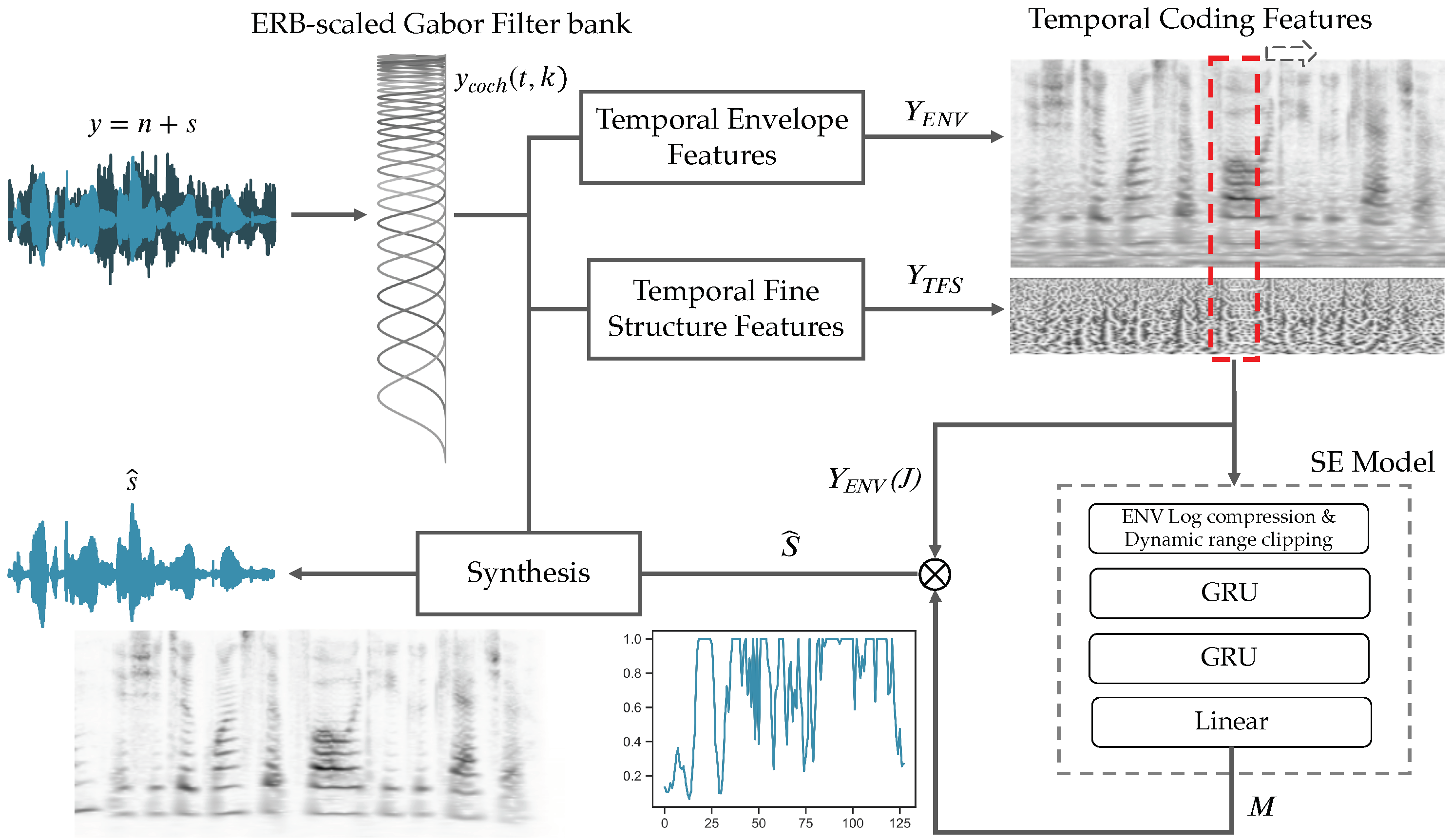
2.2. Temporal Auditory Processing: Features and Targets

In this section, we provide details and rationale about the perceptually-motivated audio signal analysis and the proposed front-end design architecture for online speech enhancement systems. Finally, we introduce a novel feature set based on temporal envelope (ENV) and temporal fine structure cues (TFS), inspired by the temporal processing mechanisms of the human auditory periphery and midbrain. Dynamically, the proposed feature extraction process effectively encodes both slow and fast temporal modulations that fall within the capabilities of the auditory system and produces a spectrogram-like representation of a speech signal.

2.2.1. ERB-Scaled Gabor Filter Bank: Analysis Framework

Established models of the peripheral filtering function of the cochlea utilize the Gammatone filter bank, which attains a balance between computational complexity and physiological accuracy [40]. The bandwidth of each auditory Gammatone filter is determined as an equivalent rectangular bandwidth (ERB), based on the linear approximation of the ERB by Glasberg and Moore (1990) [41]
E R B ( f ) = 24.7 + f 9.265   ,
where f and E R B ( f ) are in Hz. Although Gammatone-based representations exhibit the indicated behavior, regarding the temporal and spectral aspects of auditory processing, they fail to produce reconstructed signals with non-audible distortions in a direct way. Variations on Gammatone filter banks have been proposed towards a more effective analysis-synthesis framework [42]. Moreover, a perfectly invertible constant-Q transform based on nonstationary Gabor frames has been recently constructed [43]. Despite allowing for adaptable resolution of the time-frequency plane, Constant-Q transforms mismatch the auditory spectral resolution at low frequencies [44].
In this study, we propose a direct implementation of an analysis and synthesis framework for speech enhancement, which is compatible with the auditory resolution and demonstrates satisfactory intelligibility and quality of reconstructed speech signals. In particular, frequency selectivity was accounted for by a set of Gabor filters υ k that are uniformly distributed along the ERB scale (ERBS) [38]
E R B S ( f ) = 9.2645 · l n ( 1 + f 228.8455 )   .
The kernels of the analysis filter bank are defined in the frequency domain as
υ ^ k ( m ) = Γ k 1 2   · e π ( m f k Γ k ) 2 ,
where k = 0 ,   , K indexes the filterbank kernels with center frequencies f k in Hz. The effective bandwidth of υ k is determined by Γ k = E R B ( f k ) , while the factor Γ k 1 2 imposes each filter to have the same energy. This rate-place encoding is based on the recently proposed Audlet filterbank [42] and ERBlet transform [45]. In this study, we use a density of 4.55 filters per ERB, resulting in a total of K = 128 filters from 80 to 6000   Hz . Frequency bands below 80   Hz and over 6000   Hz are not considered in the analysis and were attenuated in the processed signals. Moreover, pre-emphasis and de-emphasis filters ( c = 0.97 ) were applied to audio signals at the input and output stages, respectively.

2.2.2. Temporal Envelope Features

Let y c o c h ( t , k ) denote the sub-band signal at the output of the k th ERB filter. The full-scale envelope vector y A N ( t ,   k ) is obtained by half-wave rectification followed by low-pass filtering. This is a realistic model of the signal transduction of the inner hair cells and is widely supported by auditory modelling studies [46,47]. Moreover, this approach surpasses the limitations of the Hilbert envelope [48] extraction process, by providing a framework that is efficient and valid for short observation times. The energy of the excitation signals is preserved using a weighting vector w G = ( w 1   w 2     w K 1   w K ) and the final output vector Y E N V N × K , N = L   /   τ , is resolved by integrating the envelope power over a short time window μ ( t ; τ ) = e t / τ · u ( t ) , with time constant τ = 8   ms [49]. This step can be interpreted as a down-sampling operation and is attributed to the loss of phase locking observed in the midbrain [47]. The mathematical formulation of this model can be summarized in Equations (9)–(12).
y c o c h ( t , k ) = y ( t ) υ k ( t ) ,
y A N ( t , k ) = m a x ( 0 , y c o c h ( t , k ) ) t w E ( t ) ,
y E N V = y A N · w G T ,
Y E N V ( n , k ) = ( 0 τ y E N V 2 ( n · τ + t ,   k ) · μ ( t ; τ ) d t ) 1 2 ,     n { 0 ,   , N } .
In the equations above, the · is the floor operator, n is the frame index, and w E is the impulse response of a zero-phase forward-backward low-pass filter with a cutoff frequency of 50   Hz . In favor of good signal reconstruction, we ignored all the non-linearities and adaptive mechanisms in the basilar membrane, that are attributable to the motion of the outer hair cells and the feedback communicated via the efferent system (for a detailed analysis see [50]).

2.2.3. Temporal Fine Structure Features

Even though speech intelligibility seems to depend on the acuity of slow temporal modulations, listening in the presence of noise is strongly correlated with the ability to utilize fast amplitude modulations [30], namely the perceptual cues involved in the temporal fine structure. This information is usually hindered in typical audio signal processing setups, where energy-based spectral transformations are mainly encountered, seeking a balance between time and frequency resolution. The intuition here is that spectro-temporal regions with source-dependent modulations can potentially facilitate speech enhancement systems in the identification and segregation of sound streams with similar spectral content. Hence, this stage aims to capture the temporal coding patterns associated with voicing and periodicity in a noisy speech mixture and to assess their contribution to the recovery of degraded envelope patterns.
First, a binary operator h ( · ) is applied to the filter bank output signals y c o c h . A zero-phase low-pass filter w F is then utilized to simulate the deterioration of phase-locking for frequencies above 2   kHz . Excitation signals are transformed by a lateral inhibitory network (LIN) [50] to enhance the frequency selectivity of the filter bank, mimicking the functional properties of the cochlear nucleus [51]. The LIN is simply modeled as a first-order difference with respect to the tonotopic axis, followed by a half-wave rectifier to produce y L I N [52]. The onset spikes of y L I N are obtained by time derivation and half-wave rectification. The resulting signal y S P conveys information about the inter-spike intervals between successive zero-crossings in the stimulus waveform, seeking correlates of periodicity pitch [53]. The y S P sub-band signals are finally integrated into short-time frames of τ = 8   ms , aligning to the corresponding temporal envelope features. This transformation attempts a conversion of temporal spike information into rate information, rendering a measure of TFS fluctuations in the original signal. Thus, feature values are close to zero for an unmodulated sinusoidal carrier signal, while reach higher values (close to 1) for highly modulated signals. In contrast to ENV features, this description is amplitude independent, similar to the auditory TFS coding mechanism; TFS coding is reported to be relatively level independent in the most range of above-threshold presentation levels [54,55]. The computation of the proposed temporal fine structure features can be summarized in the following sequence of operations.
y h ( t , k ) = h ( y c o c h ( t , k ) ) t w F ( t ) ,
y L I N ( t , k ) = m a x ( 0 , k y h ( t , k ) ) ,
y S P ( t , k ) = m a x ( 0 , t y L I N ( t , k ) ) ,
Y T F S ( n , k ) = Γ k 1 2 · 0 τ y S P ( n · τ + t ,   k ) d t ,
where h ( · ) is the Heaviside step function, and Y T F S denotes the final feature representation. The scaling factor Γ k 1 2 is used to normalize the feature distribution along the rate-place axis. In the current implementation, temporal fine structure encoding retains the same spectral density (4.55 channels per ERB) as the temporal envelope extraction process. TFS signals are obtained only over the low-frequency range, between 80 and 1000 Hz, where the effect of periodic cues on speech understanding is prominent. On this basis, Y T F S comprises a 59-dimensional feature vector for each short-time frame and complements Y E N V as the model input vector.

2.2.4. Synthesis Framework

The synthesis framework consists of two stages: an envelope post-processing stage and a time-domain signal reconstruction stage. First, the desired sub-band envelope gains are up-sampled to the original signal sampling rate using a causal interpolating filter to produce the vector S ^     L × K . The dynamic range of each band is then restricted to a maximum modulation depth of D r = 60   dB by a gating function and the output envelope signals are filtered for modulation frequencies below 50   Hz . Second, the sub-band temporal fine structures of the noisy mixture y T F S are modulated by the processed envelopes S ^ and a linear operator is employed to map the sub-band signals to the output audio signal s ^ .
y T F S ( t , k ) =     y c o c h ( t , k ) y E N V ( t , k ) + ϵ ,
s ^ x ( t , k ) = m a x ( S ^ ( t , k ) ,   ϵ )   t   w E ( t ) ,
s ^ ( t ) = k = 0 K ( s ^ x   y T F S ) ( t ,   k ) ,
where ϵ = 10 D r 20 .

2.3. Model Architecture & Training

In this study, we consider the causal approach for speech enhancement, where the model can access information from past time-steps and the prediction of target features is not dependent on future audio segments. A sliding rectangular window with length J in the time domain is applied to the input feature representation to enable frame-based processing. The model estimates the target features corresponding to the J t h time frame of the input representation. This approach is suitable for real-time applications, such as hearing prosthesis and audio streaming. It is also promoted by numerous other studies [16,56], as it incorporates valuable information from neighbor time-frames and reduces the redundancy of the output dimensionality, compared to sequence-to-sequence modelling [24].
Based on the above premise, let g θ : J x Λ   K denote a neural network model parameterized by the learnable parameters θ , where J determines the available temporal receptive field of the model. The parameters Λ and K denote the number of input and output features, respectively, which are determined by the desired feature representation (see Section 2.1 and Section 2.2). A two-layer gated recurrent unit (GRU) neural network with 512 units is considered as the main component of g θ . A recurrent cell processes the log-compressed input feature vector across each timestep in sequential order, and the output of the J t h step is passed to a fully-connected layer with K units. Then, the sigmoid activation function is applied to yield the final predictions. Dropout regularization with a probability of 0.4 is applied to the outputs of the recurrent layers. The prediction of the model is locally-constrained in the time domain through the parameter J , to avoid learning long-term dependencies ( > 400   ms ), leading to a more accurate and stable training procedure. This is technically achieved by setting the initial hidden state vector of the GRU to zero after each sample inference.
The model has a total of 2.71 million parameters and is trained using the Adam optimizer algorithm [57] in mini-batch mode with a batch size of 2048, to minimize the mean squared error between the target and the estimated values. The learning rate was set to 10 4 , while the learning progress was monitored by an early-stopping algorithm to avoid over-fitting to training data. The proposed speech enhancement system is depicted in Figure 1.

2.4. Dataset

Experiments were conducted on the TIMIT speech corpus of read speech [58], which is widely used for various speech tasks. It contains a total of 6300 clean utterances, spoken by 630 speakers (438 male). The speech material comes subdivided into separate training and test sets, balancing factors such as subset duration, speaker gender, phoneme occurrence, and dialectal coverage. Νo speaker or sentence appears in both partitions to avoid overlap with the training material.
The clean speech data were corrupted by various real-world and synthetic noises to form the experimental dataset. Noises were mismatched between training and test sets to ensure a legitimate experimental setup. For the training set, we selected six noise types from the UrbanSound8k dataset [59] (air conditioner, children playing, drilling, engine, gunshot, street music) with a total duration of five hours. Furthermore, training set noises were augmented by an additional 10 common noise types (ambience, babble, cafe, restaurant, street) collected from the Freesound website (http://www.freesound.org). To assess the generalization performance of the proposed approach to novel conditions, thirteen real-world noises from the DEMAND database [60] were included in the test set, recorded over a variety of environments (domestic, office, public, transportation, street, and nature). Four noise samples of the database had minimal effect on intelligibility and quality metrics even at very low signal-to-noise ratios (SNR) and thus were substituted by two common categories (speech-shaped noise and copy machine sound). All recordings were initially converted to single-channel audio clips, and were afterwards mixed with the clean speech signals of the test set. Audio files were in WAV format and were sampled at 16 kHz with a 16-bit depth.
Each speech sample is mixed in utterance level with a randomly selected noise segment, which was adjusted in level to reach a pre-defined long-term SNR, based on the energy of active speech regions. For the training and validation set, the SNR values were sampled from a uniform distribution between −5 and 3 dB. To assist the presentation and interpretability of the results, the test set audio mixtures were obtained in discrete SNRs {−8, −6, −4, −2, 0, 2, 4, 6} dB, following a uniform distribution. Silent regions longer than one second were detected and excluded/discarded from clean speech samples before the mixing procedure, using an energy-based voice activity detector.

2.5. Objective Evaluation Criteria

We evaluated the performance of the proposed approach in terms of intelligibility and perceptual quality based on four well-known objective metrics that reflect the aspects of normal and impaired auditory perception.
The enhancement of speech intelligibility for normal-hearing listeners is evaluated through the extended short-term objective intelligibility (eSTOI) measure. The eSTOI (ranging from 0 to 1) is able to objectively quantify the intelligibility of speech obscured by temporally modulated noises and noisy signals processed with time-frequency weighting for a group of normal-hearing listeners [61]. The eSTOI algorithm incorporates spectral correlation of short-time segments (384-ms) by comparing the energy-normalized spectrograms of processed and clean speech signals. Prior to the computation of the intelligibility score, pauses between sentences are removed from both reference and processed audio signals. The temporal envelopes of one-third octave frequency bands (15 frequency bands from 150 Hz to 4.3 kHz) are then approximated by summing the corresponding STFT coefficient energies.
The eSTOI measure is complemented by the full reference algorithm of the PESQ score, as defined in the ITU-T P.862 standard [62]. PESQ estimates the subjective mean opinion score for a group of normal-hearing listeners regarding the perceived audio quality over telephone networks, when degraded by speech or noise distortions. It ranges from −0.5 (or 1.0 in most cases) to 4.5 and is widely used to assess speech processing algorithms [2,21,56,63], indicating the speech quality measurement of enhanced speech.
Moreover, the hearing-aid speech perception index (HASPI) [64] and the hearing-aid sound quality index (HASQI) [65] are employed to objectively evaluate the model performance for listeners with various degrees of hearing loss. These metrics (both ranging from 0 to 1) rely on hearing profile-dependent auditory model representations to compute the long-term correlations between reference and processed speech signals. HASPI incorporates changes in the low-, mid- and high-intensity regions of the spectral envelope and the harmonic structure to construct a viable model of consonant and vowel perception for hearing-impaired listeners. On the other hand, the HASQI metric combines aspects of linear filtering and non-linear distortions found in a hearing device to measure the sound quality of a processed signal as perceived by a hearing aid user. In this study, six generic hearing loss profiles (Figure 2) are considered to simulate the evaluation of sound quality and perception for hearing-impaired listeners [66]. For both metrics, the reference signal presentation level was set to 65 dB SPL (corresponding to signal RMS value of 1), while clean, noisy, and enhanced speech signals were imposed to equal RMS values.

2.6. Experimental Setup

The experimental setup comprises three speech enhancement systems, namely the ENV, the ENV-TFS and the reference STFT system. The ENV-TFS system is trained to predict the M c mask representation ( γ = 1 ) of Κ = 128 clean speech envelope features, as described in Section 2.2.2, by processing Λ = 187 auditory coding features of noisy speech mixture (128 ENV features and 59 TFS features). The relative contribution of TFS features to the system performance is evaluated by assessing the model when having access to solely ENV information ( Λ = Κ = 128 ). Finally, the baseline STFT method employs the conventional IRM as a target and the log-scaled magnitude spectrogram (Equation (5)) as the model input. Features are obtained by the STFT of size 512 ( 31.25   ms ) with a 50% overlap and the Hann window function. Frequency bins between 80 and 6000 Hz ( Λ = Κ = 256 ) are considered to match the ENV and ENV-TFS systems. The same model architecture is employed in all setups, to ensure a fair comparison between the three systems. The only difference lies in the linear output layer; the number of output units is determined by the desired output dimensionality Κ . The source code of the experimental procedure along with the complete set of results on the TIMIT dataset is freely available at the dedicated online repository (https://doi.org/10.5281/zenodo.4028860).

3. Results

3.1. Reconstruction from Envelope Spectrogram

The first 100 speech signals of the TIMIT test set were employed for the evaluation of the proposed analysis-synthesis framework. The intelligibility and quality of reconstructed acoustic waveforms are evaluated through the eSTOI and PESQ objective metrics, and are compared to the reference STFT-based analysis framework.
Results are depicted in Table 1, where three scenarios are considered. First, clean speech signals are transformed into time-frequency representations (denoted as ENV and STFT) and are synthesized back using the corresponding synthesis function. Results indicate that the proposed approach preserves intelligibility and quality of the reconstructed speech signal, with minimal loss compared to the perfectly-reconstructed speech signals obtained via the STFT. The second and third cases consider the ideal case where the speech enhancement model unerringly estimates the target feature representation, indicating the maximum perceptual gain that can be achieved in each case. To simulate this, the soft mask M c is applied to the noisy feature representation to obtain the ideally processed speech signals in the context of masking-based speech enhancement. In detail, ENV and STFT methods have a maximum capacity of increasing eSTOI by 34% and 36%, respectively, and speech quality by 1.52 and 1.87 PESQ units. Clipping the target mask M c to be between 0 and 1, with the use of the upper bound parameter γ , results in a small decrease in the maximum capacity of both methods. The above results provide a validation of the proposed envelope feature representation for speech enhancement. An auditory-motivated envelope representation is provided which is accommodated by sufficient speech reconstruction quality and intelligibility, close to the reference STFT analysis.

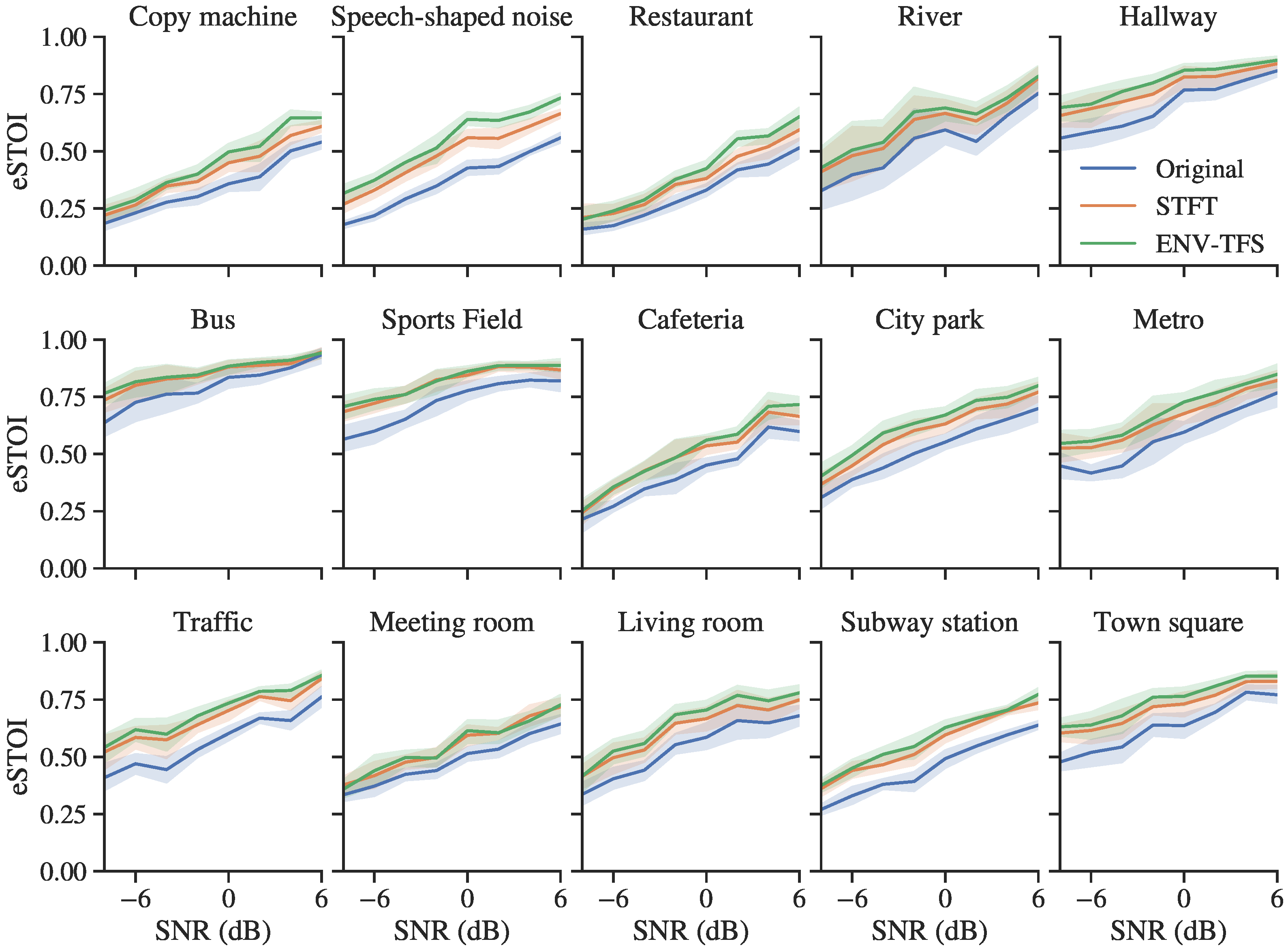
3.2. Objective Evaluation for Normal-Hearing Listeners

In this section, we evaluate the performance of the utilized GRU model in a typical masking-based speech enhancement setup, in terms of objective metrics for intelligibility and perceived quality for normal-hearing listeners. Table 2 shows the predicted intelligibility and quality results averaged over all SNRs and noises. It is apparent that all methods improved the eSTOI and PESQ scores relative to unprocessed noisy speech. Mean intelligibility scores were higher for the ENV-TFS method compared to the baseline STFT method, with improvements ranging from 2.5% to 3.5%. Marginally higher (0.02) mean PESQ scores are also observed across different SNR values.
The effect of TFS features on the model performance is assessed further. The ENV-TFS system led to improvements for eSTOI (3%) and PESQ (0.05) mean scores compared to the ENV system, using the same model architecture. The performance of the ENV system matches the STFT approach in most conditions for normal-hearing listeners. Moreover, ENV and ENV-TFS methods motivate a narrower receptive field ( 48   ms ) compared to the best performing STFT model with a temporal receptive field of 176   ms (10 time-steps).
The performance of the ENV-TFS approach across different SNRs can be depicted in Figure 3. Intelligibility and quality scores vary significantly across SNR values. Similar performance to seen and unseen SNR conditions is observed, indicating a strong generalization ability of the model. The utilized processing led to increased intelligibility for the 99.1% of speech utterances. Moreover, PESQ scores were improved for 99.9% of the samples. The ENV-TFS model provided better intelligibility results (eSTOI) than the STFT-based model for the 65% of test set samples, while no significant advantage can be reported for either method in terms of perceived quality for normal hearing-listeners (PESQ).
As shown in Figure 4, these results were consistent across all noise types. The utilized GRU-based speech processing facilitated a solid increase in objective intelligibility for the majority of noise conditions. In most cases, the proposed approach performed considerably better than the STFT-based model. Performance gains for the proposed approach were evident in highly modulated acoustic environments (cafeteria, town square, living room, copy machine). At the same time, marginal improvements over the baseline system are observed in noises of a steadier nature (Subway, bus, river) and in SNRs where the original signals already feature adequate intelligibility (>0.75).

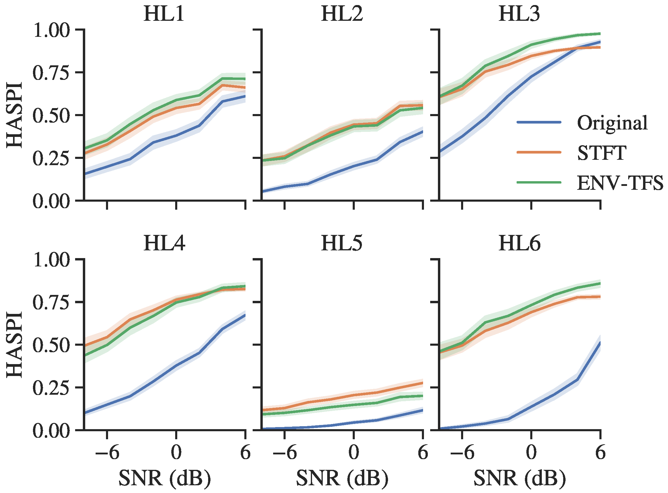
3.3. Objective Evaluation for Hearing-Impaired Listeners

The performance of speech enhancement approaches is evaluated for six typical hearing loss configurations (presented in Figure 2). The processed and unprocessed noisy utterances of the TIMIT test set were compared to the corresponding clean speech samples via HASPI and HASQI models. Table 3 shows the objective intelligibility (HASPI) and quality (HASQI) values between the proposed ENV-TFS system and the conventional STFT system. Mean values of both HASPI and HASQI measures were improved in all test conditions. In detail, simulation results indicate that ENV-TFS approach yields better results for HL1, HL3 and HL6 compared to the STFT approach. In contrast, results on the hearing loss configurations HL2 and HL4 indicate similar or slightly lower performance of the proposed speech enhancement system. Lower results were obtained for the HL5 configuration. The proposed algorithm improved HASPI and HASQI values for the 94.6% and 98.2% of test set samples, respectively. Predicted intelligibility results of the ENV-TFS system were higher than the STFT for the 55% of test set samples, while HASQI values were lower for the 54% of test set samples.
Moreover, the HASPI values across different SNR conditions can be depicted in Figure 5. Processed signals yield improved intelligibility scores by 14–30% across different SNR values. The total values were slightly higher at SNRs of 0, −2, and −4 dB for both ENV-TFS and STFT methods. In addition, the generalization ability of the models to unseen SNR condition is also validated, as HASPI and HASQI differences were not significant. Finally, the above results indicate that the conventional and the proposed methods were comparable at this stage and the performance of each approach is highly dependent on the degree and configuration of the simulated audiograms.

4. Discussion

In this study, we investigated the performance of deep learning-based speech enhancement algorithms on vocoder-based processing of speech. The method introduces a novel feature set on the basis of recent findings on peripheral auditory processing and embeds these attributes into an effective speech analysis/synthesis framework. Features are designed to capture temporal modulation information from sub-band audio signals and extract low-dimensionality attributes from short-time audio segments. The processing method applies to causal inference systems, while providing an alternative to conventional spectrum-wise speech analysis frameworks. It features sufficiently low latency on inference, even with no available hardware acceleration for the implemented digital filters. The computational processing time was slightly below T / 2 , where T is the duration of an audio segment, running on a standard personal computer equipped with the Intel core i7-7700 processor (3.6 GHz base frequency).
A simple two-layer GRU-based neural network architecture was employed to model the temporal envelope dynamics of degraded speech signals. The network accepts temporal envelope and fine structure features for a short-time segment. Then, it computes the mask vector for the low frequency amplitude modulations of speech. A generalization of the widely used IRM is exploited on this account, adapting to arbitrary feature representations. This target is intuitive and general, as it can be adopted by any algorithm that concerns masking-based audio source separation and enhancement. In addition, the GRU architecture offers advantages over alternative architectures, such as fully-connected deep neural networks or long short-term memory networks, due to the fewer learned parameters for the same receptive field, a more stable training procedure, and good generalization to novel noises. Nevertheless, speech enhancement performance was not substantially affected by the employed architecture, given proper network configuration. The deployed GRU model architecture consists of two hidden layers, each with a size of 512. This model provided superior performance for all employed representations, while pairwise differences of the proposed and baseline systems were not significantly affected by the model hyperparameters. Thus, a high level of consistency in the results was observed across different experimental model parameterizations.
Based on our experimental results, it can be concluded that gated recurrent unit neural network architectures have indeed potential to increase speech intelligibility and perceived quality in a wide range of real-world conditions, given a modest amount of training data and sufficient computational power. To our knowledge, this method is the first approach based on established auditory-motivated methods that provides an alternative to raw waveform or spectrum-wise processing for deep learning-based speech enhancement. The proposed temporal auditory-motivated features effectively encode both slow and fast amplitude modulations, providing thus valuable information to the speech enhancement models, which are otherwise obscured in usual spectral representations. In the future, dynamic processing of both low-frequency and high-frequency amplitude modulations of speech, i.e., the temporal fine structure of degraded speech signals could enhance the proposed methodology and provide an intuitive and complete speech analysis framework based on modulation cues.

5. Conclusions

In this study, we propose a novel set of auditory-motivated features for single-channel speech enhancement by fusing temporal envelope and temporal fine structure information in the context of vocoder-like processing. In order to investigate the potential of temporal auditory coding features on the enhancement of speech intelligibility, we employ a GRU neural network to recover the low-frequency amplitude modulations of speech. Experimental results showed that the proposed features achieved improvements compared to the conventional log-scaled magnitude spectrogram, in terms of objective metrics for intelligibility and perceptual quality of normal-hearing listeners. Mixed results were observed regarding simulated listeners with hearing loss. Both the proposed and standard approaches significantly increased the personalized objective metrics for intelligibility and perceived quality, while the expediency of each method is postulated to mainly depend on the audiogram type. Finally, the exploited framework applies to causal speech processing systems, as it provides valuable feature representation with sufficient intelligibility and quality of reconstructed speech signals.

Author Contributions

Conceptualization, I.T. and G.P.; methodology, I.T. and L.V.; validation, I.T., L.V. and D.M.; data curation, L.V.; writing—original draft preparation, Ι.Τ. and L.V.; writing—review and editing, I.T., L.V. and D.M.; visualization, D.M.; supervision, G.P. All authors have read and agreed to the published version of the manuscript.

Funding

This research received no external funding.

Conflicts of Interest

The authors declare no conflict of interest.

References

  1. Pardede, H.; Ramli, K.; Suryanto, Y.; Hayati, N.; Presekal, A. Speech Enhancement for Secure Communication Using Coupled Spectral Subtraction and Wiener Filter. Electronics 2019, 8, 897. [Google Scholar] [CrossRef] [Green Version]
  2. Rix, A.W.; Hollier, M.P.; Hekstra, A.P.; Beerends, J.G. Perceptual Evaluation of Speech Quality (PESQ) The New ITU Standard for End-to-End Speech Quality Assessment Part I—Time-Delay Compensation. J. Audio Eng. Soc. 2002, 50, 755–764. [Google Scholar]
  3. Srinivasan, S.; Roman, N.; Wang, D. Binary and ratio time-frequency masks for robust speech recognition. Speech Commun. 2006, 48, 1486–1501. [Google Scholar] [CrossRef]
  4. Czyzewski, A.; Kulesza, M. Speech Codec Enhancements Utilizing Time Compression and Perceptual Coding. In Audio Engineering Society Convention 122; Audio Engineering Society: New York, NY, USA, 2007. [Google Scholar]
  5. Park, G.; Cho, W.; Kim, K.-S.; Lee, S. Speech Enhancement for Hearing Aids with Deep Learning on Environmental Noises. Appl. Sci. 2020, 10, 6077. [Google Scholar] [CrossRef]
  6. Loizou, P.C. Speech Enhancement: Theory and Practice; CRC Press: Boca Raton, FL, USA, 2013; ISBN 1466504218. [Google Scholar]
  7. Boll, S. Suppression of acoustic noise in speech using spectral subtraction. IEEE Trans. Acoust. 1979, 27, 113–120. [Google Scholar] [CrossRef] [Green Version]
  8. Tsoukalas, D.E.; Mourjopoulos, J.; Kokkinakis, G. Perceptual filters for audio signal enhancement. J. Audio Eng. Soc. 1997, 45, 22–36. [Google Scholar]
  9. Ephraim, Y.; Malah, D. Speech enhancement using a minimum-mean square error short-time spectral amplitude estimator. IEEE Trans. Acoust. 1984, 32, 1109–1121. [Google Scholar] [CrossRef] [Green Version]
  10. Purwins, H.; Li, B.; Virtanen, T.; Schlüter, J.; Chang, S.; Sainath, T. Deep Learning for Audio Signal Processing. IEEE J. Sel. Top. Signal Process. 2019, 13, 206–219. [Google Scholar] [CrossRef] [Green Version]
  11. Korvel, G.; Kurowski, A.; Kostek, B.; Czyzewski, A. Speech analytics based on machine learning. In Machine Learning Paradigms; Springer: Cham, Switzerland, 2019; pp. 129–157. [Google Scholar]
  12. Vrysis, L.; Tsipas, N.; Thoidis, I.; Dimoulas, C. 1D/2D Deep CNNs vs. Temporal Feature Integration for General Audio Classification. J. Audio Eng. Soc. 2020, 68, 66–77. [Google Scholar] [CrossRef]
  13. Vryzas, N.; Vrysis, L.; Matsiola, M.; Kotsakis, R.; Dimoulas, C.; Kalliris, G. Continuous Speech Emotion Recognition with Convolutional Neural Networks. J. Audio Eng. Soc. 2020, 68, 14–24. [Google Scholar] [CrossRef]
  14. Vrysis, L.; Thoidis, I.; Dimoulas, C.; Papanikolaou, G. Experimenting with 1D CNN Architectures for Generic Audio Classification. In Audio Engineering Society Convention 148; Audio Engineering Society: New York, NY, USA, 2020. [Google Scholar]
  15. Thoidis, I.; Giouvanakis, M.; Papanikolaou, G. Audio-based detection of malfunctioning machines using deep convolutional autoencoders. In Audio Engineering Society Convention 148; Audio Engineering Society: New York, NY, USA, 2020. [Google Scholar]
  16. Goehring, T.; Keshavarzi, M.; Carlyon, R.P.; Moore, B.C.J. Using recurrent neural networks to improve the perception of speech in non-stationary noise by people with cochlear implants. J. Acoust. Soc. Am. 2019, 146, 705–718. [Google Scholar] [CrossRef] [PubMed] [Green Version]
  17. Lee, G.W.; Kim, H.K. Multi-Task Learning U-Net for Single-Channel Speech Enhancement and Mask-Based Voice Activity Detection. Appl. Sci. 2020, 10, 3230. [Google Scholar] [CrossRef]
  18. Czyzewski, A.; Kostek, B.; Bratoszewski, P.; Kotus, J.; Szykulski, M. An audio-visual corpus for multimodal automatic speech recognition. J. Intell. Inf. Syst. 2017, 49, 167–192. [Google Scholar] [CrossRef] [Green Version]
  19. Chen, J.; Wang, Y.; Yoho, S.E.; Wang, D.; Healy, E.W. Large-scale training to increase speech intelligibility for hearing-impaired listeners in novel noises. J. Acoust. Soc. Am. 2016, 139, 2604–2612. [Google Scholar] [CrossRef] [PubMed] [Green Version]
  20. Lang, H.; Yang, J. Speech enhancement based on fusion of both magnitude/phase-aware features and targets. Electronics 2020, 9, 1125. [Google Scholar] [CrossRef]
  21. Bae, S.H.; Choi, I.; Kim, N.S. Disentangled feature learning for noise-invariant speech enhancement. Appl. Sci. 2019, 9, 2289. [Google Scholar] [CrossRef] [Green Version]
  22. Rao, A.; Carney, L.H. Speech enhancement for listeners with hearing loss based on a model for vowel coding in the auditory midbrain. IEEE Trans. Biomed. Eng. 2014, 61, 2081–2091. [Google Scholar] [CrossRef] [Green Version]
  23. Oord, A.v.D.; Dieleman, S.; Zen, H.; Simonyan, K.; Vinyals, O.; Graves, A.; Kalchbrenner, N.; Senior, A.; Kavukcuoglu, K. Wavenet: A generative model for raw audio. arXiv 2016, arXiv:1609.03499. [Google Scholar]
  24. Thoidis, I.; Vrysis, L.; Pastiadis, K.; Markou, K.; Papanikolaou, G. Investigation of an encoder-decoder lstm model on the enhancement of speech intelligibility in noise for hearing impaired listeners. In Audio Engineering Society Convention 146; Audio Engineering Society: New York, NY, USA, 2019. [Google Scholar]
  25. Rosen, S.; Carlyon, R.P.; Darwin, C.J.; Russell, I.J. Temporal information in speech: Acoustic, auditory and linguistic aspects. Philos. Trans. R. Soc. London. Ser. B Biol. Sci. 1992, 336, 367–373. [Google Scholar] [CrossRef]
  26. Van Tasell, D.J.; Soli, S.D.; Kirby, V.M.; Widin, G.P. Speech waveform envelope cues for consonant recognition. J. Acoust. Soc. Am. 1987, 82, 1152–1161. [Google Scholar] [CrossRef]
  27. Souza, P.E.; Wright, R.A.; Blackburn, M.C.; Tatman, R.; Gallun, F.J. Individual sensitivity to spectral and temporal cues in listeners with hearing impairment. J. Speech Lang. Hear. Res. 2015, 58, 520–534. [Google Scholar] [CrossRef] [Green Version]
  28. Shannon, R.V.; Zeng, F.-G.; Kamath, V.; Wygonski, J.; Ekelid, M. Speech recognition with primarily temporal cues. Science 1995, 270, 303–304. [Google Scholar] [CrossRef]
  29. Grose, J.H.; Mamo, S.K.; Hall III, J.W. Age effects in temporal envelope processing: Speech unmasking and auditory steady state responses. Ear Hear. 2009, 30, 568. [Google Scholar] [CrossRef] [Green Version]
  30. Hopkins, K.; Moore, B.C.J. The contribution of temporal fine structure to the intelligibility of speech in steady and modulated noise. J. Acoust. Soc. Am. 2009, 125, 442–446. [Google Scholar] [CrossRef] [PubMed]
  31. Koutsogiannaki, M.; Francois, H.; Choo, K.; Oh, E. Real-Time Modulation Enhancement of Temporal Envelopes for Increasing Speech Intelligibility. Interspeech 2017, 1973–1977. [Google Scholar] [CrossRef] [Green Version]
  32. Langhans, T.; Strube, H. Speech enhancement by nonlinear multiband envelope filtering. In Proceedings of the ICASSP’82. IEEE International Conference on Acoustics, Speech, and Signal Processing, Paris, France, 3–5 May 1982; Volume 7, pp. 156–159. [Google Scholar]
  33. Apoux, F.; Tribut, N.; Debruille, X.; Lorenzi, C. Identification of envelope-expanded sentences in normal-hearing and hearing-impaired listeners. Hear. Res. 2004, 189, 13–24. [Google Scholar] [CrossRef]
  34. Anderson, M.C.; Arehart, K.H.; Kates, J.M. The effects of noise vocoding on speech quality perception. Hear. Res. 2014, 309, 75–83. [Google Scholar] [CrossRef]
  35. Shetty, H.N. Temporal cues and the effect of their enhancement on speech perception in older adults—A scoping review. J. Otol. 2016, 11, 95–101. [Google Scholar] [CrossRef] [PubMed] [Green Version]
  36. Shetty, H.N.; Mendhakar, A. Deep band modulation and noise effects: Perception of phrases in adults. Hear. Balance Commun. 2015, 13, 111–117. [Google Scholar] [CrossRef]
  37. Wang, D.; Chen, J. Supervised speech separation based on deep learning: An overview. IEEE ACM Trans. Audio Speech Lang. Process. 2018, 26, 1702–1726. [Google Scholar] [CrossRef] [PubMed]
  38. Moore, B.C.J.J.; Glasberg, B.R. A revision of Zwicker’s loudness model. Acta Acust. United Acust. 1996, 82, 335–345. [Google Scholar]
  39. Maganti, H.K.; Matassoni, M. Auditory processing-based features for improving speech recognition in adverse acoustic conditions. EURASIP J. Audio Speech Music Process. 2014, 2014, 21. [Google Scholar] [CrossRef] [Green Version]
  40. Chou, K.F.; Dong, J.; Colburn, H.S.; Sen, K. A Physiologically Inspired Model for Solving the Cocktail Party Problem. J. Assoc. Res. Otolaryngol. 2019, 20, 579–593. [Google Scholar] [CrossRef] [PubMed] [Green Version]
  41. Glasberg, B.R.; Moore, B.C.J. Derivation of auditory filter shapes from notched-noise data. Hear. Res. 1990, 47, 103–138. [Google Scholar] [CrossRef]
  42. Necciari, T.; Holighaus, N.; Balazs, P.; Průša, Z.; Majdak, P.; Derrien, O. Audlet filter banks: A versatile analysis/synthesis framework using auditory frequency scales. Appl. Sci. 2018, 8, 96. [Google Scholar] [CrossRef] [Green Version]
  43. Velasco, G.A.; Holighaus, N.; Dörfler, M.; Grill, T. Constructing an invertible constant-Q transform with nonstationary Gabor frames. In Proceedings of the 14th International Conference on Digital Audio Effects (DAFx), Paris, France, 19–23 September 2011; Volume 33, pp. 93–100. [Google Scholar]
  44. Abolhassani, M.D.; Salimpour, Y. A human auditory tuning curves matched wavelet function. In Proceedings of the 2008 30th Annual International Conference of the IEEE Engineering in Medicine and Biology Society, Vancouver, BC, Canada, 20–24 August 2008; pp. 2956–2959. [Google Scholar]
  45. Necciari, T.; Balazs, P.; Holighaus, N.; Søndergaard, P.L. The ERBlet transform: An auditory-based time-frequency representation with perfect reconstruction. In Proceedings of the 2013 IEEE International Conference on Acoustics, Speech and Signal Processing, Vancouver, BC, Canada, 26–31 May 2013; pp. 498–502. [Google Scholar]
  46. Apoux, F.; Millman, R.E.; Viemeister, N.F.; Brown, C.A.; Bacon, S.P. On the mechanisms involved in the recovery of envelope information from temporal fine structure. J. Acoust. Soc. Am. 2011, 130, 273–282. [Google Scholar] [CrossRef]
  47. Chi, T.; Ru, P.; Shamma, S.A. Multiresolution spectrotemporal analysis of complex sounds. J. Acoust. Soc. Am. 2005, 118, 887–906. [Google Scholar] [CrossRef] [Green Version]
  48. Gabor, D. Theory of communication. Part 1: The analysis of information. J. Inst. Electr. Eng. III Radio Commun. Eng. 1946, 93, 429–441. [Google Scholar] [CrossRef] [Green Version]
  49. Sheft, S.; Yost, W.A. Temporal integration in amplitude modulation detection. J. Acoust. Soc. Am. 1990, 88, 796–805. [Google Scholar] [CrossRef]
  50. Wang, K.; Shamma, S. Self-normalization and noise-robustness in early auditory representations. IEEE Trans. Speech Audio Process. 1994, 2, 421–435. [Google Scholar] [CrossRef]
  51. Yang, X.; Wang, K.; Shamma, S.A. Auditory representations of acoustic signals. IEEE Trans. Inf. Theory 1992, 38, 824–839. [Google Scholar] [CrossRef] [Green Version]
  52. Elhilali, M.; Shamma, S.A. A cocktail party with a cortical twist: How cortical mechanisms contribute to sound segregation. J. Acoust. Soc. Am. 2008, 124, 3751–3771. [Google Scholar] [CrossRef] [PubMed] [Green Version]
  53. Cariani, P. Temporal coding of periodicity pitch in the auditory system: An overview. Neural Plast. 1999, 6. [Google Scholar] [CrossRef] [PubMed]
  54. Palmer, A.R.; Russell, I.J. Phase-locking in the cochlear nerve of the guinea-pig and its relation to the receptor potential of inner hair-cells. Hear. Res. 1986, 24, 1–15. [Google Scholar] [CrossRef]
  55. Ewert, S.D.; Paraouty, N.; Lorenzi, C. A two-path model of auditory modulation detection using temporal fine structure and envelope cues. Eur. J. Neurosci. 2020, 51, 1265–1278. [Google Scholar] [CrossRef] [PubMed]
  56. Cui, X.; Chen, Z.; Yin, F. Speech enhancement based on simple recurrent unit network. Appl. Acoust. 2020, 157, 107019. [Google Scholar] [CrossRef]
  57. Kingma, D.P.; Ba, J.L. Adam: A method for stochastic optimization. arXiv 2014, arXiv:1412.6980. [Google Scholar]
  58. Zue, V.; Seneff, S.; Glass, J. Speech database development at MIT: TIMIT and beyond. Speech Commun. 1990, 9, 351–356. [Google Scholar] [CrossRef]
  59. Salamon, J.; Jacoby, C.; Bello, J.P. A dataset and taxonomy for urban sound research. In Proceedings of the 22nd ACM international conference on Multimedia, Orlando, FL, USA, 3–7 November 2014; pp. 1041–1044. [Google Scholar]
  60. Thiemann, J.; Ito, N.; Vincent, E. The diverse environments multi-channel acoustic noise database: A database of multichannel environmental noise recordings. J. Acoust. Soc. Am. 2013, 133, 3591. [Google Scholar] [CrossRef]
  61. Jensen, J.; Taal, C.H. An algorithm for predicting the intelligibility of speech masked by modulated noise maskers. IEEE/ACM Trans. Audio Speech Lang. Process. 2016, 24, 2009–2022. [Google Scholar] [CrossRef]
  62. ITU-T P.862.2 Wideband extension to Recommendation P.862 for the assessment of wideband telephone networks and speech codecs. Telecommun. Stand. Sect. ITU 2007, 12. [CrossRef]
  63. Beerends, J.G.; Hekstra, A.P.; Rix, A.W.; Hollier, M.P. Perceptual evaluation of speech quality (pesq) the new itu standard for end-to-end speech quality assessment part ii: Psychoacoustic model. J. Audio Eng. Soc. 2002, 50, 765–778. [Google Scholar]
  64. Kates, J.M.; Arehart, K.H. The hearing-aid speech perception index (HASPI). Speech Commun. 2014, 65, 75–93. [Google Scholar] [CrossRef]
  65. Kates, J.M.; Arehart, K.H. The hearing-aid speech quality index (HASQI) version 2. AES J. Audio Eng. Soc. 2014, 62, 99–117. [Google Scholar] [CrossRef]
  66. Thoidis, I.; Vrysis, L.; Markou, K.; Papanikolaou, G. Development and evaluation of a tablet-based diagnostic audiometer. Int. J. Audiol. 2019, 58, 476–483. [Google Scholar] [CrossRef]
Publisher’s Note: MDPI stays neutral with regard to jurisdictional claims in published maps and institutional affiliations.
Figure 1. Detailed illustration of the components of the proposed speech enhancement inference algorithm. The input signal is filtered by an ERB filter bank. The outputs y c o c h are transformed to auditory-motivated temporal envelope and fine structure representations. The Speech Enhancement (SE) model processes J frames on every iteration and predicts the envelope gains of the J t h frame. Predictions are used to modulate the unprocessed envelopes, and the enhanced audio waveform s ^ is synthesized using the sub-band y c o c h signals.
Electronics 09 01698 g001
Figure 2. Typical hearing loss audiograms incorporated in the objective evaluation of sound quality and intelligibility using HASPI and HASQI measures. These include two high-frequency hearing loss audiograms (HL1: blue, HL2: orange), two mild hearing loss audiograms (HL3: yellow, HL4: purple), one moderate hearing loss (HL5: green), and one low-frequency hearing loss (HL6: cyan).
Electronics 09 01698 g002
Figure 3. eSTOI (a) and PESQ (b) scores for eight SNR values (−8 dB to 6 dB) averaged over all noises of the test dataset. The box-whisker plots outline the objective results corresponding to the original noisy speech mixtures of the test dataset, the enhanced audio mixtures by the ENV-TFS system, and the enhanced audio mixtures by the STFT system.
Electronics 09 01698 g003
Figure 4. Objective intelligibility scores of the utilized speech enhancement systems in different noise types. The sub-figures illustrate the mean eSTOI scores (with shaded confidence interval 95%) for the proposed system (ENV-TFS), the baseline system (STFT) and the unprocessed samples (Original) with respect to different SNR values.
Electronics 09 01698 g004
Figure 5. Illustrated comparison of HASPI scores between the proposed (ENV-TFS) and conventional (STFT) speech enhancement systems across different SNR values (from −8 to 6 dB) for the HL1–6 simulated audiograms.
Electronics 09 01698 g005
Table 1. Objective speech intelligibility (eSTOI) and quality (PESQ) results between the standard STFT and the proposed ENV analysis-synthesis frameworks. Mean and standard deviation values are presented for the first 100 utterances of the TIMIT test set.
MethodeSTOIPESQ
ENVSTFTENVSTFT
Noisy (unprocessed)0.54 ± 0.170.54 ± 0.171.19 ± 0.151.19 ± 0.15
Target M c   ( γ = ) 0.88 ± 0.050.90 ± 0.052.73 ± 0.253.11 ± 0.37
Target M c   ( γ = 1 ) 0.86 ± 0.060.89 ± 0.052.71 ± 0.253.06 ± 0.37
Clean (reconstructed)0.99 ± 0.001.00 ± 0.003.90 ± 0.174.20 ± 0.15
Table 2. Objective speech intelligibility (eSTOI) and quality (PESQ) results for normal-hearing listeners between the ENV, the ENV-TFS and the STFT-based speech enhancement systems.
MethodeSTOIPESQ
Original0.529 ± 0.201.101 ± 0.16
STFT0.608 ± 0.201.668 ± 0.48
ENV0.610 ± 0.191.638 ± 0.51
ENV-TFS0.635 ± 0.201.687 ± 0.49
Table 3. Objective speech perception (HASPI) and quality (HASQI) results (mean ± standard deviation in percentage) for six typical hearing loss audiograms between the STFT and the ENV-TFS systems, compared to the original noisy speech mixtures.
HASPI HASQI
Config.OriginalSTFTENV-TFSOriginalSTFTENV-TFS
HL136.5 ± 28.449.0 ± 27.153.0 ± 29.314.3 ± 9.024.0 ± 12.626.8 ± 13.0
HL219.4 ± 17.940.0 ± 24.338.8 ± 25.911.2 ± 6.425.7 ± 12.122.8 ± 10.2
HL363.5 ± 31.578.8 ± 21.283.7 ± 25.020.6 ± 12.034.5 ± 16.535.4 ± 17.3
HL435.0 ± 25.469.7 ± 23.167.3 ± 27.915.6 ± 8.333.5 ± 14.229.9 ± 13.4
HL54.6 ± 6.419.2 ± 14.214.3 ± 13.66.6 ± 4.928.7 ± 9.919.7 ± 7.7
HL615.8 ± 23.964.1 ± 24.068.3 ± 28.05.1 ± 6.019.0 ± 7.422.4 ± 8.7
Publisher’s Note: MDPI stays neutral with regard to jurisdictional claims in published maps and institutional affiliations.

