Self-Supervised Learning to Increase the Performance of Skin Lesion Classification

Abstract

To successfully train a deep neural network, a large amount of human-labeled data is required. Unfortunately, in many areas, collecting and labeling data is a difficult and tedious task. Several ways have been developed to mitigate the problem associated with the shortage of data, the most common of which is transfer learning. However, in many cases, the use of transfer learning as the only remedy is insufficient. In this study, we improve deep neural models training and increase the classification accuracy under a scarcity of data by the use of the self-supervised learning technique. Self-supervised learning allows an unlabeled dataset to be used for pretraining the network, as opposed to transfer learning that requires labeled datasets. The pretrained network can be then fine-tuned using the annotated data. Moreover, we investigated the effect of combining the self-supervised learning approach with transfer learning. It is shown that this strategy outperforms network training from scratch or with transfer learning. The tests were conducted on a very important and sensitive application (skin lesion classification), but the presented approach can be applied to a broader family of applications, especially in the medical domain where the scarcity of data is a real problem.

1. Introduction

Deep learning algorithms have achieved a tremendous success in various image processing tasks. Currently, deep learning-based approaches obtain state-of-the-art performance in vision tasks such as image classification [1], object localization and detection [2,3,4], as well as object segmentation [5].

It is well-known that any deep learning system requires a lot of annotated data to obtain satisfying results [6]. In some cases, publicly available datasets can be used to train the network. However, in many domains collecting data is difficult, since the availability of applicable datasets is limited. For instance, collecting medical data is difficult due to law restrictions and privacy politics [7]. Moreover, datasets used for supervised training have to be labeled manually. Although in most cases it might be done by a non-skilled worker, some areas, e.g., medicine, require high-level domain expertise to annotate the data, which makes the process very expensive and time consuming.

One of the common remedies to this problem is the use of transfer learning [8]. Transfer learning involves training the network on a huge dataset (e.g., Imagenet) [9] and then treating this network as a starting point in the target task training. This method can provide a performance improvement. However, due to differences in the character of the dataset used for the pretraining and that of the target task, it cannot be fully utilized. Nevertheless, transfer learning is currently one of the most commonly used practices in many domains. A different approach taken in this paper, which bears the name of self-supervised learning [10], consists of introducing a pretraining stage in the form of learning the features from unlabeled datasets.

In general, self-supervised learning is a family of techniques that pretrain the network to learn visual features. In contrast to transfer learning, self-supervised pretraining does not require a labeled dataset. 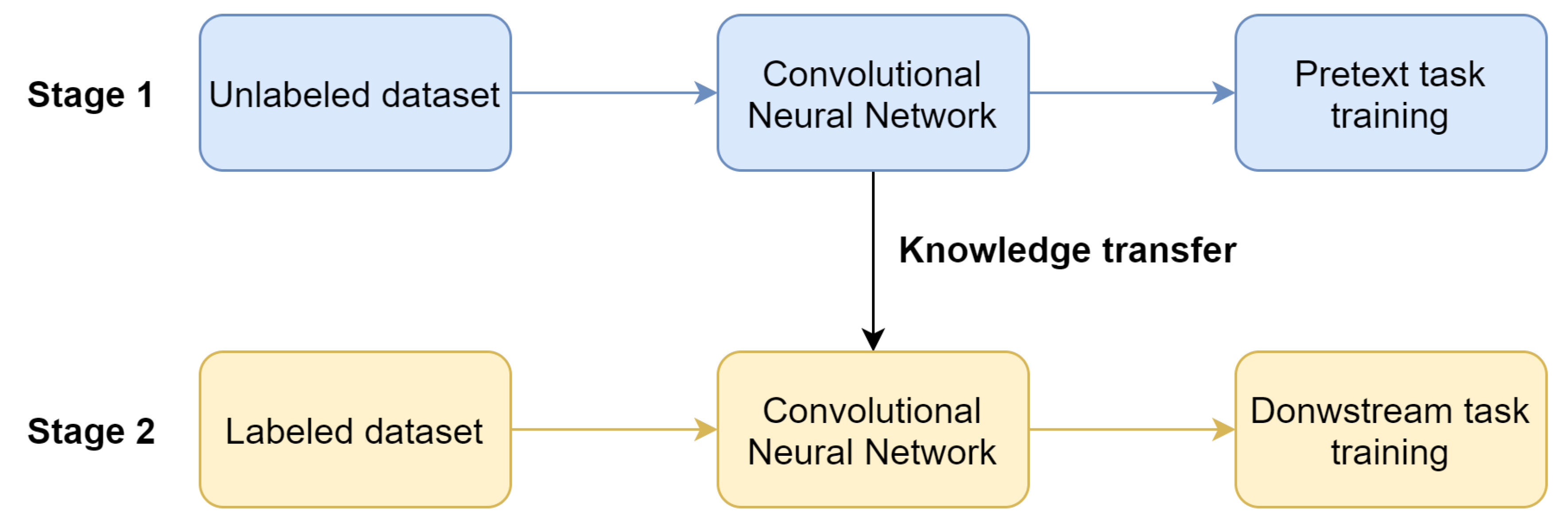This is very useful in a variety of tasks in which a large part of available datasets is not annotated (e.g., in medicine) or training dataset is artificially generated without accompanying labels [11]. The use of the self-supervised learning method involves two steps (Figure 1): pretraining of the network with the use of unlabeled data (pretext task) and training on the target task with labeled data (downstream task). Moreover, pretext task training does not require any external human supervision. Hence, the unlabeled data can be used to increase the performance of the system.

Pretext task training is performed to learn visual features that can be utilized in downstream task training. It is performed on an unlabeled dataset, which eliminates the expensive and time-consuming labeling process. The common pipeline in pretext task training is to apply the transformation to the image, and then make the network to predict the transformation parameter. For instance, one can rotate an image and then teach the network to predict the rotation angle [12]. To perform such a task, the network needs to learn higher-level features.

The type of the pretext task determines the choice of the objective function used during the training. For example, when the network task is to predict the rotation angle from a predefined set of possible rotation angles, the task becomes a classification problem that can be trained using standard cross-entropy loss. Recently, methods relying on contrastive loss have attracted researchers’ attention, as they allow obtaining decent results [13,14,15]. The general purpose of contrastive losses is to make image representations and their modification similar, while making representations of the image and other images in the dataset different.

The majority of works introducing novel self-supervised algorithms are evaluated on well-known benchmark datasets that usually contain millions of labeled images. Although testing on benchmark datasets is essential in the development of new methods and allows the field to progress, there is also a need to test algorithms in real-world applications. Unlike benchmark datasets, many practical tasks involve training on small and poorly balanced datasets [16,17].

This paper proposes to incorporate transfer learning into self-supervised learning-based pretraining in the scarce dataset scenario. This strategy leads to superior results that outperform those obtained using transfer learning or self-supervised learning alone. The performance of the method is investigated on the dataset provided with the ISIC2017 challenge; the skin lesion classification problem [18]. The deployment of a skin lesion classification model is a challenging task [19], due to the limited size of the dataset that contains only 2000 training images. It is shown that the system trained on such a small dataset can still benefit from deploying a self-supervised strategy. Self-supervised learning is compared with standard approaches i.e., training from scratch and training with the use of transfer learning.

The presented findings are believed to bring advantages in a variety of domains, especially in those where the researchers have to cope with a small amount of data.

The remaining part of the paper is organized as follows: Section 2 outlines related works, while in Section 3, a general approach to the method is presented. The used dataset is described in Section 4, and selected details of the method are presented in Section 5. Section 6 gives the description of the experiments, and Section 7 concludes the paper.

2. Related Work

Self-supervised learning has recently emerged as a solution to utilize unlabeled samples during neural networks training. The advantage of self-supervised methods is the ability to learn useful representation without a need for manually labeled examples. It enables incorporating unlabeled examples to perform network pretraining.

A variety of methods have been proposed that differ in the kinds of used pretext tasks and objective functions.

Generation-based methods involve learning representations by networks that learn to generate some content. The authors of [20] propose an architecture that restores the content of the randomly chosen patch removed from the image. In turn, Larsson et al. [21] proposes image colorization as a form of the pretext task. Images in the dataset are converted to grayscale, then the task of the network is to restore full information about the color. Context-based pretext tasks rely on the semantic and spatial information within the image. The authors of one of the first methods of this kind proposed a pretext task which involves the prediction of relative positions of two patches within the image [22]. The image is divided into nine square tiles arranged in a 3 × 3 grid. The network task is to predict the position of a randomly chosen tile relatively to the central patch. Thus, this pretext task comes down to a multi-class classification problem. The authors of [23] built upon that work and proposed to shuffle patches and make the network predict the shuffle pattern.

In [12] Gitaris et al. propose a network called RotNet. The dataset used during pretext task training is created by performing random rotations to images. The network task is to predict the rotation angle. Although it can be easily implemented, the method provides a significant improvement.

DeepCluster proposed in [24] uses a clustering algorithm to group representations into clusters. Next, those groups are utilized during supervised training. Thus, the training involves alternating between clustering the representations into a group and training the network to predict which group the image belongs to.

Approaches based on contrastive losses have recently shown great potential. This family of methods involves applying modification to the image. The network is trained in such a way as to make representations of two different views of the image similar, while making those views dissimilar to other examples in the dataset. This approach makes the representations to become invariant under transformation applied to the images. It was shown that the quality of the learned representations benefits from such a form of pretraining.

Numerous methods based on contrastive loss were proposed, including: [14,15,25]. The PIRL (Pretext-Invariant Representation Learning) method [13], upon which this paper is built, makes use of contrastive loss to obtain invariance property. To reduce the amount of computation performed by the algorithm, the authors of the method introduced the memory bank that stores representations of all images in the dataset.

Numerous studies have reported successful applications of deep neural networks to the task of skin lesion classification. The authors of [26] reached dermatologist-level classification performance using the network based on Inception architecture [27] trained on huge dataset of skin lesion images (about 100 k). The author of [28] evaluated different network ensembling methods, showing that an ensemble significantly increases classification performance. Barata et al. [29] developed a complex skin lesion classification system composed of attention modules and LSTM cells that allows for hierarchical classification and decision interpretation in the form of heatmaps. The authors of [30] proposed an attention residual learning convolutional neural network that can adaptively focus on the discriminative parts of the skin lesion picture. The influence of different deep learning methods on skin lesion classification was evaluated in [31].

3. Approach

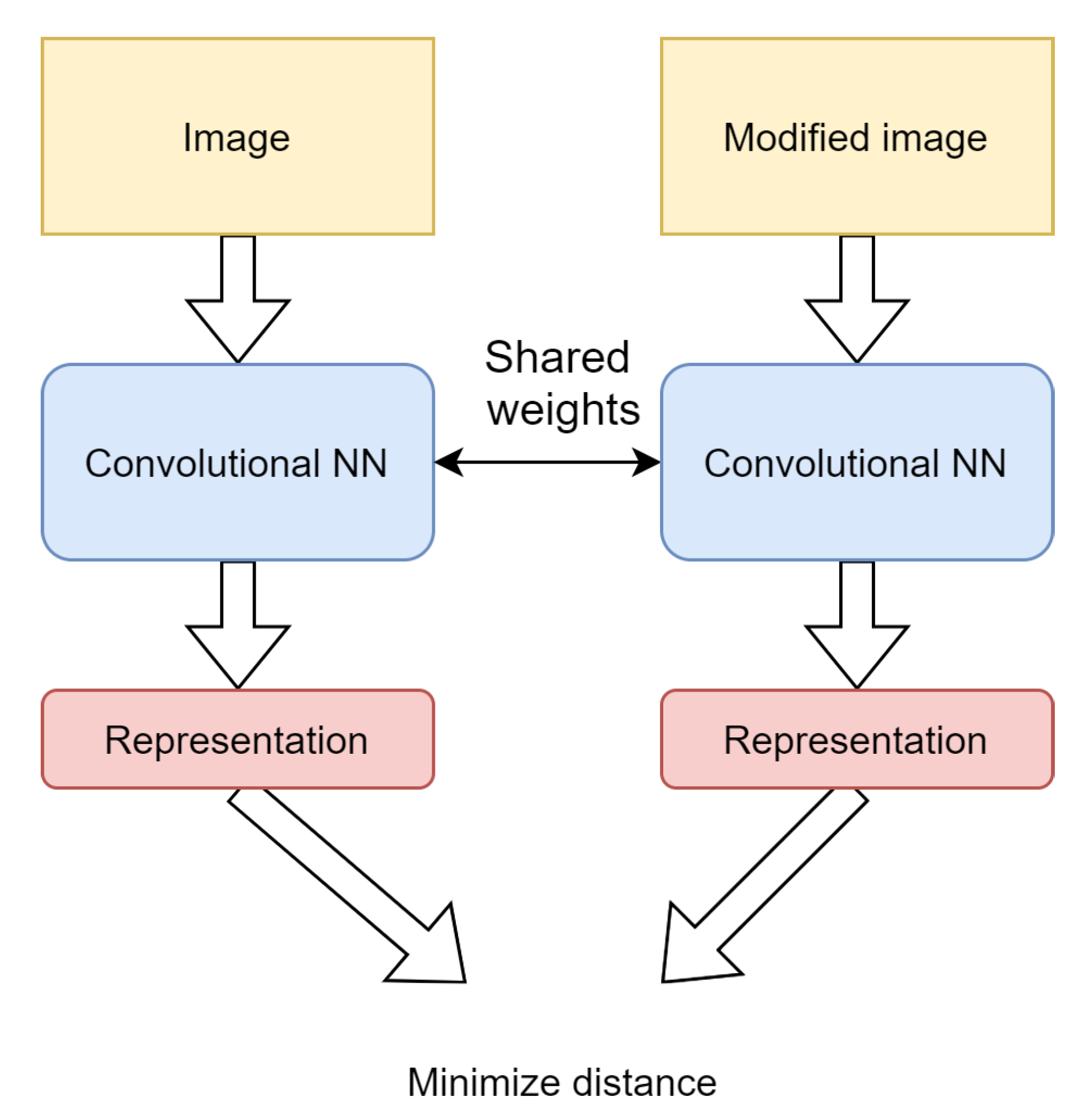
This section outlines the PIRL algorithm adopted to solve the problem of skin lesion analysis. The algorithm is described in full detail in [13]. The main aim of the method is to pretrain the network in such a way as to make semantic representations produced by the network to be invariant under different image transformations (Figure 2). In other words, the representations of different views of the image should be similar. It was shown that such representations increase the network performance on the downstream task [32]. The objective function from the family of contrastive losses [33] enables these requirements to be satisfied.

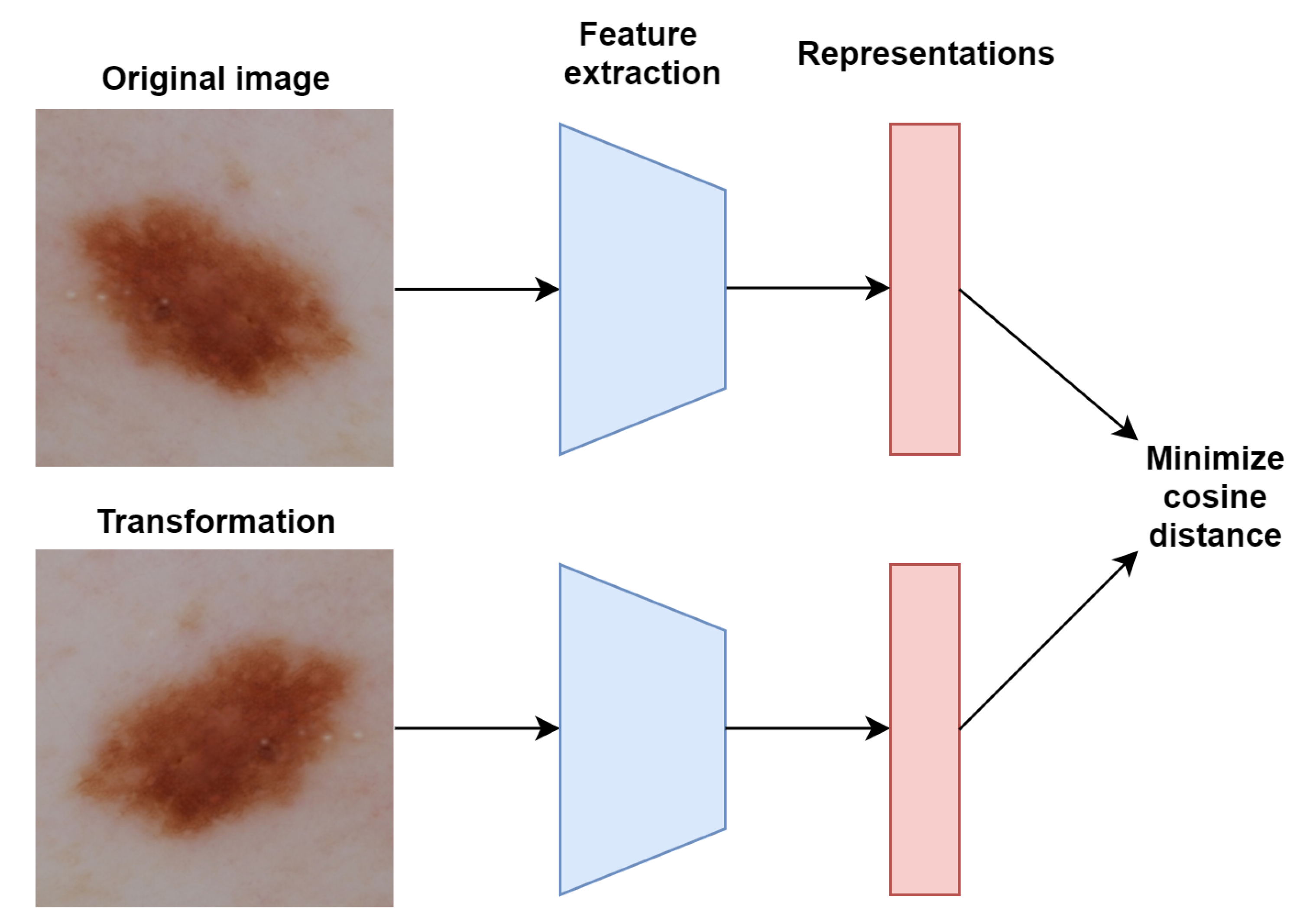
Loss Function

The objective function aims to maximize the similarity of representations of the image and its transformation (positive examples). The similarity is represented by a cosine distance. Moreover, in order to avoid trivial solutions, the loss function encourages the network to produce different representations of the given image and other images in the dataset (negative examples). The contrastive loss function that satisfies those requirements has the following form:

$$L_{NCE}=-log\left(\frac{exp\left(\frac{s({\mathbf{v}}_{\mathbf{I}},{\mathbf{v}}_{{\mathbf{I}}^t})}{\tau }\right)}{exp\left(\frac{s({\mathbf{v}}_{\mathbf{I}},{\mathbf{v}}_{{\mathbf{I}}^t})}{\tau }\right)+{\sum }_{I^{\prime }\in {\mathcal{D}}_N}exp\left(\frac{s({\mathbf{v}}_{{\mathbf{I}}^t},{\mathbf{v}}_{{\mathbf{I}}^{\prime }})}{\tau }\right)}\right)$$

(1)

where:

• ${\mathbf{v}}_{\mathbf{I}}$, ${\mathbf{v}}_{{\mathbf{I}}^t}$—representations of the image and its transformation,
• $s(·)$—cosine similarity,
• $\tau$—temperature coefficient,
• $I^{\prime }$—set of negative examples drawn uniformly from the dataset,
• ${\mathbf{v}}_{{\mathbf{I}}^{\prime }}$—representation of the negative example,
• $D_N$—dataset.

To facilitate the interpretation of the loss function, one can consider the term inside the log function as a softmax function. Minimization of $L_{NCE}$ function leads to the maximization of similarity between the original and transformed images (nominator), and minimization of similarities between the transformed image and other images from the dataset (denominator). As a result, the trained network maps the original image and the modified one to neighboring representations, while mapping different images to non-neighboring representations.

Prior works on contrastive self-supervised learning have shown that the number of negative examples in I’ set has significant impact on the quality of trained representations [25,34]. Studies have reported performance improvement with the increased number of negative examples representations used in loss calculation. A naive approach is to produce representations of negative samples each time the batch is provided to the network. However, this approach is time consuming due to many forward propagations of the algorithms to produce representations of negative examples. To mitigate this problem, in [13] the authors of the PIRL method proposed utilization of a memory bank that stores the representation of each image in the dataset. This significantly reduced the computation effort needed for running the algorithm by limiting the number of required forward propagations. The representations stored in the memory are the exponential running averages of original images produced in preceding epochs.

The introduction of the memory bank enables the introduction of the loss function that consists of linear combination of two terms:

$$L(I,I^t)=\lambda L_{NCE}({\mathbf{m}}_{\mathbf{I}},{\mathbf{v}}_{{\mathbf{I}}^t})+(1-\lambda )L_{NCE}({\mathbf{m}}_{\mathbf{I}},{\mathbf{v}}_{\mathbf{I}})$$

(2)

where:

• I, $I^t$—image and its transformation,
• ${\mathbf{v}}_{\mathbf{I}}$, ${\mathbf{v}}_{{\mathbf{I}}^t}$—representations of the image and its transformation,
• ${\mathbf{m}}_{\mathbf{I}}$—representation stored in the memory,
• $\lambda$—loss weight coefficient.

The first term relates to the similarity of the representation stored in the memory bank with that of the modified image produced by the network. Moreover, it measures the similarity of the representation of the transformed image to other images. This form is equivalent to the original loss, except for the fact that representations of the original image and other images are taken from the memory bank. The second term compares the representation of the original image stored in the bank with that produced by the network in the current epoch – this term stabilizes the training process by avoiding rapid weight changes. Moreover, it compares the representations of the unmodified image with other images and tries to make them dissimilar during the optimization process.

4. Dataset

The performance of the self-supervised pretraining was assessed on the task of skin lesion classification. This task involves classifying the dermoscopic images of lesions into two classes: benign and malignant.

The dataset used in the experiments was provided in the ISIC2017 challenge [18]. This dataset contains images of lesions collected from clinical centers using a variety of devices. The dataset contains 2000 training, 150 validation, and 600 testing images. Each set is divided into two classes—malignant and benign and has the same class ratio (benign—80 percent of images, malignant 20 percent of images).

The classes in the dataset are not well-balanced, there are far more images of benign than malignant lesions. This is a common difficulty when analyzing medical datasets, as the number of people with a particular disease is much smaller than that of healthy patients, or patients with other diseases (other classes). Moreover, the images from different classes can be very similar to each other. These properties of the datasets make correct diagnosis a challenging task, even for a highly-skilled specialist [35]. In addition, different specialists often provide a different diagnosis for the same case.

Like other medical problems, the problem of skin lesion diagnosis significantly differs from classification based on standard benchmark datasets, where the number of images is high, and classes are well-balanced and can be easily distinguished by a human with nearly perfect accuracy.

5. Implementation Details

While Section II outlined a general approach to the method, this section provides implementation details of the employed application. The performed experiments made use of two transformation strategies: Rotation transformation [12], and Jigsaw transformation [23], during pretext task training. Each pretext task involved preparation of the image I and its transformation $I^t$ to produce their representations. The way that I and $I^t$ were produced depended on the given pretext task.

In order to validate the presented approach, we decided to take advantage of the ResNet50 [36] architecture as a feature extraction backbone, as it is commonly accepted architecture to evaluate self-supervised algorithms. Moreover, ResNet50 is a network with proven effectiveness in numerous studies, including medical applications considered in this paper. Specifically, we used ResNet50 implementation provided in the Pytorch [37] library that produces a 2048-dimensional feature vector as the output of the last average pooling layer. This vector was further reduced to the lower dimension of 128 that was then provided to the loss function. The reduction methods differed depending on the pretext task used.

5.1. Initial Preprocessing

The images in the dataset vary in size and aspect ratio. Moreover, the areas of lesion take up a different size on the images. To adapt images to the fixed input size of the network, the following initial image preprocessing is performed.

First, lesions from the images are segmented using segmentation masks provided by the organizer of the challenge. The shape of the lesion is an indicator of malignancy; thus, it is essential to keep original proportions of the lesion in the image. Therefore, square image patches are cropped with the lesion inside, and then those images are resized to the fixed size of $400\times 400$ pixels. This image is further modified depending on the pretext task.

5.2. Jigsaw Pretext Task

Jigsaw pretext task involves comparing the original image representation I with the representation $I^t$ produced by a combination of representations of 9 tiles extracted from the original image (Figure 3).

These 9 tiles are produced in the following way. The preprocessed image of size 400 × 400 is resized to 255 × 255 and split into a 3 × 3 grid consisting of nine 85 × 85-pixel tiles. Then, a 64 × 64 segment is cropped randomly from each 85 × 85 tile. Data augmentation is independently applied to each tile, including color jittering, and random vertical and horizontal flips. The term “independently” means that a different set of data augmentation parameters is drawn for each tile to introduce more diversity in the dataset. Finally, each tile is normalized to have zero mean and unit variance.

The original image is produced in the following way. The preprocessed image is resized to the size of $224\times 224$. Then, standard data augmentation methods including color jittering, random horizontal and vertical flips are applied. Finally, the image is normalized to have zero mean and unit variance. In order to produce the representation of image I, a linear fully-connected layer is placed after the average pooling layer with the 128-dimensional output size. The original image is passed through the network to obtain its representation.

To produce the representation of the modified image $I^t$, nine patches are passed through the network to produce nine 128-dimensional vectors corresponding to each tile. Next, the vectors are concatenated in random order to produce the 1152-dimensional vector. This vector is then provided to the next linear fully-connected layer to produce a 128- dimensional vector. Finally, this vector is used in the loss function as the representation of the modified image $I^t$.

Rotation Pretext Task

The preparation of the original image I and its transformation $I^t$ is much simpler than in the Jigsaw pretext task (Figure 4). The first steps are the same for both I and $I^t$. The preprocessed image is resized to 300 × 300, next two images of size 224 × 224 are randomly cropped to form both I and $I^t$. Random color jittering and normalization are applied to both images independently. Finally, the modified image $I^t$ is rotated by an angle randomly selected from the set of (0, 90, 180, 270) degrees.

In order to obtain the 128-dimensional representation, a fully connected linear layer is placed after the average pooling layer. Finally, both images are passed through the network to produce representations of the modified and original images, both of 128 size.

5.3. Pretext Task Training

Pretext task training is performed with the use of contrastive loss (1) described in previous sections. Stochastic Gradient Descent (SGD) with momentum algorithm is used as an optimizer, with the learning rate set to 0.001, momentum coefficient set to 0.9, and the batch size set to 32. Weight decay was disabled during the pretraining. For each image in the batch, 1000 negative examples are sampled from the memory bank. The temperature coefficient in the loss function is set to 0.07, which is the value commonly used in other applications. The coefficient between two loss terms is set to 0.5. The training lasts 1000 epochs.

The representations stored in the memory bank are the moving exponential averages with the update coefficient set to 0.5. This makes the features from last epochs to have the strongest influence on the value of features stored in the memory bank. Before training, all images are passed to the network to initialize the memory bank with the initial set of representations.

5.4. Downstream Task Training

Once the pretext task training is completed, the obtained weights can be utilized during the downstream task training. The layers used to produce 128-dimensional representations are dropped, leaving average pooling as the last layer. A sigmoid neuron is placed at the top of the network, because the task of lesion classification is a two-class classification problem. The network is trained with binary cross-entropy as the loss function. Stochastic Gradient Descent (SGD) with momentum algorithm is used as an optimizer, with the learning rate set to 0.001, momentum coefficient set to 0.9, and the batch size set to 32. The early stopping procedure was applied to prevent overfitting.

6. Experiments

A series of experiments were performed to evaluate the proposed methods. Six different ways of neural network training were tested, including standard training from scratch and training using transfer learning. The parameters of the training were the same as described in the pretext task training section, the approaches differed only in weight initialization. Transfer learning and training from scratch are the baseline approaches, which were used for comparison with self-supervised learning approaches. The performance of the network pretrained on Jigsaw and Rotation pretext tasks using contrastive loss was checked. Finally, the influence of the incorporation of transfer learning into self-supervised pretraining was evaluated. Specifically, the network that performs pretext task was not initialized from scratch, instead it was initialized using transfer learning from ImageNet. Pretext task pretraining was performed on the whole training set without labels. Then the whole dataset was used to perform downstream tasks, transfer learning, and training from scratch. Each experiment was repeated five times and the average was taken to obtain more reliable results. The area under Receiver Operating Characteristic curve (ROC AUC) was taken as the main performance measure, as it is widely used in medical applications. Moreover, accuracy (ACC) and area under precision-recall curve (PR AUC) are reported. The results are collated in

Table 1. Results of using self-supervised learning.

Method	ROC AUC	PR AUC	ACC
Random initialization	0.598	0.257	79.67
Transfer learning (TF)	0.791	0.525	83.03
TF + Jigsaw	0.830	0.595	84.47
Jigsaw	0.664	0.321	79.80
TF + Rotation	0.826	0.591	84.00
Rotation	0.732	0.370	80.30

.

We can observe that transfer learning achieves superior results over random initialization. This is the expected outcome, as transfer learning is a commonly known method to increase network performance. We can also see that incorporating self-supervised methods without transfer learning allows to increase the results over random initialization. However, these results are worse than those obtained using transfer learning. The best results have been achieved by combining transfer learning with self-supervised learning. Transfer learning with the Jigsaw pretext task allows obtaining ROC AUC of 0.830, which shows significant improvement over transfer learning alone (0.791). These results illustrate the benefits of the use of both methods in image recognition system deployment.

To directly evaluate the quality of extracted image features we decided to apply an approach similar to linear evaluation protocol, reported in numerous papers. According to this protocol, first, we freezed pretrained CNN weights, next we generated 2048 dimensional features vectors that we provided to the selected classifier. We analyzed the effectiveness using the Support Vector Machine (SVM) algorithm with a radial basis function as a kernel, k-nearest neighbors (k-NN) algorithm with 4 neighbors, random forest classifier with the maximum number of trees set to 50, and finally a sigmoid neuron (

Table 2. The evaluation of the quality of extracted image features.

Method	Classifier	ROC AUC	PR AUC	ACC
Random initialization	k-NN	0.582	0.244	0.785
	Sigmoid Neuron	0.597	0.247	0.778
	Random forest	0.572	0.243	0.801
	SVM	0.599	0.260	0.805
Transfer learning (TF)	k-NN	0.700	0.388	0.778
	Sigmoid Neuron	0.748	0.434	0.793
	Random forest	0.727	0.368	0.803
	SVM	0.796	0.461	0.815
TF + Jigsaw	k-NN	0.680	0.420	0.808
	Sigmoid Neuron	0.758	0.446	0.800
	Random forest	0.708	0.390	0.812
	SVM	0.776	0.489	0.829
Jigsaw	k-NN	0.600	0.243	0.752
	Sigmoid Neuron	0.678	0.318	0.765
	Random forest	0.682	0.320	0.789
	SVM	0.675	0.313	0.801
TF + Rotation	k-NN	0.761	0.482	0.815
	Sigmoid Neuron	0.797	0.552	0.820
	Random forest	0.748	0.451	0.815
	SVM	0.814	0.581	0.851
Rotation	k-NN	0.676	0.314	0.768
	Sigmoid Neuron	0.704	0.359	0.792
	Random forest	0.680	0.331	0.803
	SVM	0.740	0.391	0.800

).

The performed experiments have shown that a combination of self-supervised learning and transfer learning leads to superior results over transfer learning alone for all the examined classifiers (Table 2). Please note that due to this approach, the classification results are worse than they could have been without freezing the weights of pretrained backbone. Typically, in practical applications weights of the backbone are fine-tuned during the optimization process, leading to higher results.

To simulate the situation where the available dataset is even more scarce, the performance of the algorithms was evaluated using only a fraction of the training set. Specifically, self-supervised pretraining was performed on the whole training set, then the network was trained on the fraction of the training set. In particular, 1% (20 images) and 10% (200 images) were randomly drawn from the training set to pretrain the network. The batch size was set to 4 when the network was trained on 20 images. The sizes of the validation and test sets remained the same as in the previous experiments. The results are reported in

Table 3. Training on 20 images (1% of the training set).

Method	ROC AUC	PR AUC	ACC
Random initialization	0.555	0.230	79.30
Transfer learning (TF)	0.519	0.201	80.70
TF + Jigsaw	0.666	0.327	80.53
Jigsaw	0.599	0.252	79.33
TF + Rotation	0.755	0.395	81.50
Rotation	0.658	0.310	79.53

and

Table 4. Training on 200 images (10% of the training set).

Method	ROC AUC	PR AUC	ACC
Random initialization	0.493	0.201	79.30
Transfer learning (TF)	0.734	0.405	80.70
TF + Jigsaw	0.753	0.416	80.53
Jigsaw	0.638	0.265	79.33
TF + Rotation	0.780	0.458	81.50
Rotation	0.698	0.361	79.53

.

The ROC AUC scores in Table 3 show that the use of transfer learning on such a small training set (20 images) causes the network to barely learn anything. However, the combination of transfer learning and self-supervised learning allows for obtaining satisfying performance of of 0.755 ROC AUC. The results are quite impressive, taking into account the very small number of training examples.

The training on 200 labeled images was also performed, which is a relatively common dataset size in many domains (Table 4).

The results are similar to the previous experiments, where transfer learning with Rotation pretext task provided the best performance. Importantly, training on 10% of the training set with transfer learning and rotation pretext task leads to similar results as when the transfer learning is used with the 100% of the training set. This results shows that the less training data we have, the greater benefits of applying the proposed approach.

The reported results were obtained with downstream training performed without the application of data augmentation. Therefore, we decided to add data augmentation during downstream task training. Data augmentation included random crops, flips rotations, and color jittering. The results are presented in

Table 5. Training on 2000 images (whole dataset) with data augmentation.

Method	ROC AUC	PR AUC	ACC
Transfer learning (TF)	0.825	0.587	84.10
TF + Jigsaw	0.835	0.607	83.33
TF + Rotation	0.842	0.613	85.17

. Confusion matrices are presented in

Table 6. Confusion matrix—TF (transfer learning) with data augmentation.

		Predicted Label
		Benign	Malignant
True label	Benign	446	37
	Malignant	59	59

,

Table 7. Confusion matrix—TF + Jigsaw with data augmentation.

		Predicted Label
		Benign	Malignant
True label	Benign	439	45
	Malignant	55	62

and

Table 8. Confusion matrix—TF + Rotation with data augmentation.

		Predicted Label
		Benign	Malignant
True label	Benign	453	30
	Malignant	59	58

.

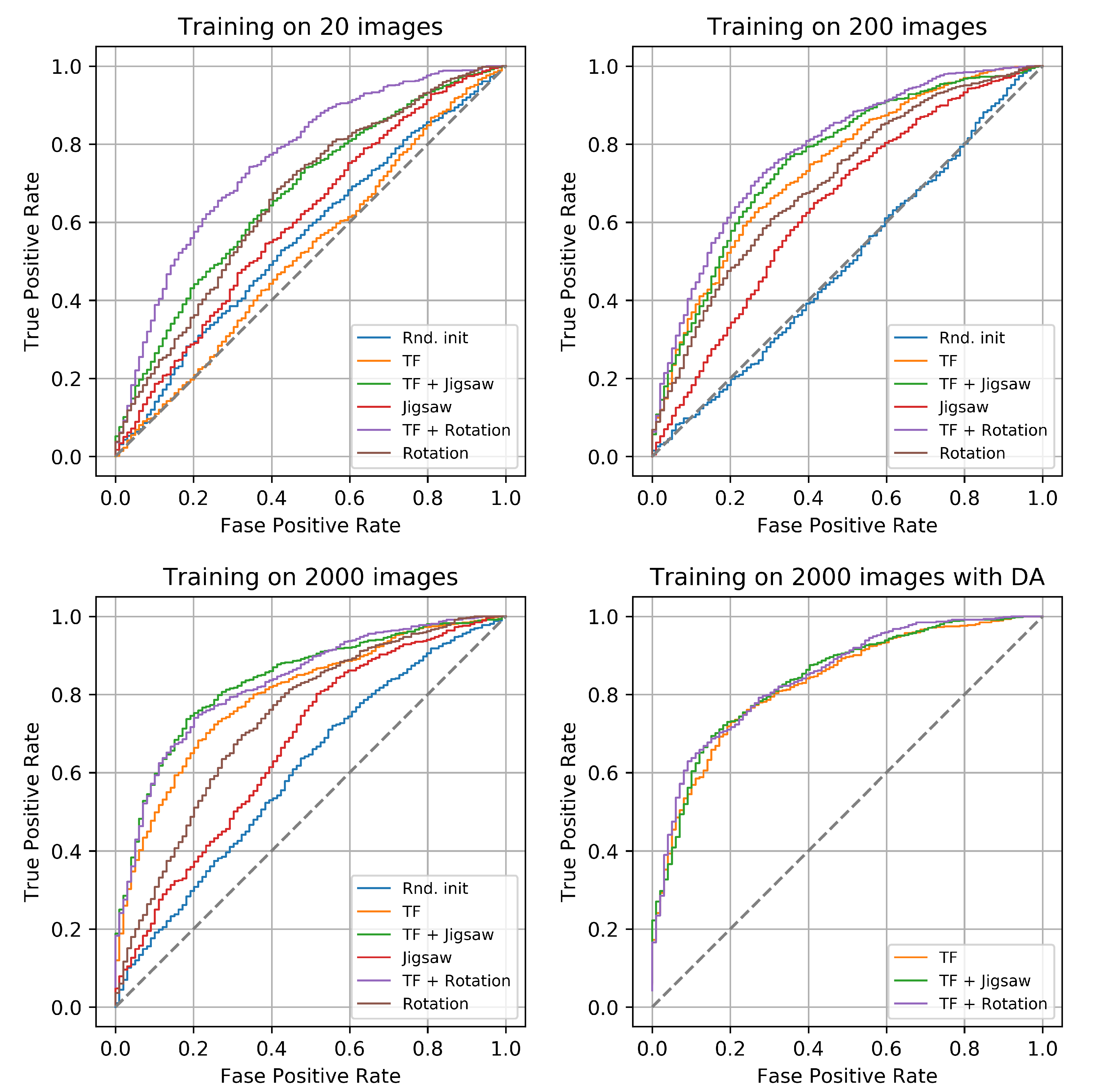
The utilization of richer data augmentation leads to much better performance. Once again, self-supervised pretraining in combination with transfer learning leads to superior performance. However, the gap between transfer learning and transfer learning with self-supervised methods is smaller in this case. The ROC curves for evaluated settings are shown in Figure 5.

The use of self-supervised learning and transfer learning allowed to achieve nearly top-level AUC score in the ISIC2017 challenge. The results obtained by the three top solutions are 0.868, 0.856, and 0.874, while ROC AUC achieved in the present study is 0.852. The comparison with other works is presented in

Table 9. Comparison with other works on the ISIC 2017 dataset.

Network	ROC AUC
VGG16 [28]	0.766
VGG16 [29]	0.800
ResNet50 [28]	0.757
ResNet50 [29]	0.775
ResNet50 [38]	0.868
ResNet50 [39]	0.870
DenseNet161 [40]	0.818
DenseNet161 [29]	0.800
ResNet50—TF + Jigsaw—ours	0.835
ResNet50—TF + Rotation—ours	0.842
ResNet50— Ensemble—ours	0.856

.

Despite the fact that the presented result is not the best, it was obtained by single ResNet50 architecture without additional modules (e.g., custom heads), modifications (e.g., polar pooling), or ensemble of many networks. Our pipeline involves only simple data augmentation, without complex data preprocessing or methods, such as test time augmentation, to increase the final performance. Moreover, we did not use any external data to train the networks, as other participants did [18]. The reported work highlights the algorithmic efficacy of the proposed solution.

During the training process, training of each method was repeated five times to obtain more reliable results. Those networks can be used in a cheap way to increase the performance by model ensembling [31,41]. The output of all networks trained with full data augmentation was averaged, which led to the improvement in both accuracy and ROC AUC to 86.16% and 0.856, respectively.

7. Conclusions

In this paper, performance of the self-supervised learning technique under small and unbalanced dataset conditions, was studied and reported. The proposed approach, being the combination of transfer learning with self-supervised learning, has led to significant increase of the accuracy and ROC AUC scores. It was shown that the PIRL algorithm tested previously on huge benchmark datasets can be successfully applied in practical tasks where only a small number of labeled images is provided. Our research results show that self-supervised pretraining can be beneficial even in cases when the full dataset is labeled.

The network performance was tested using different ways of weight initialization: random initialization, transfer learning, self-supervised learning, and combination of transfer learning with self-supervised learning. Two pretext tasks: Jigsaw and Rotation were evaluated. The proposed solution, which is the combination of self-supervised learning with transfer learning, gave the best results in all considered scenarios. The trainings with very small datasets with only 20 and 200 images have shown data efficiency of the proposed method. The research clearly showed that the less training data we have, the greater benefits of applying the proposed approach. The network pretrained on 2000 unlabeled images, then trained on 200 labeled images reached almost the same performance as the network trained on 2000 labeled images using transfer learning. Moreover, it has been shown that the proposed approach allows to obtain classification results by a single network, similar to those obtained by complex deep learning systems. This shows high effectiveness of the method.

The conducted experiments have shown high efficiency of proposed method, that achieve superior results over transfer learning applied alone. The research clearly showed that the less training data we have, the greater benefits of applying the proposed approach.

The conducted research allowed to state that the proposed method might be a remedy to the small training set problem. Self-supervised learning can be beneficial in many areas where only small amount of data is available, or annotation of dataset is expensive. Self-supervised learning enables to incorporate an unlabeled dataset in training.

Our future work in this field will focus on development of pretext tasks that include labels during pretraining. Additionally, we would like to test self-supervised learning approach using more complex architectures (e.g., ResNeXt, SE-ResNet), different data augmentation pipelines (e.g., coarse dropout), and ensemble methods.

References

- Tan, M.; Le, Q.V. EfficientNet: Rethinking Model Scaling for Convolutional Neural Networks. In Proceedings of the 36th International Conference on Machine Learning, ICML 2019, Long Beach, CA, USA, 9–15 June 2019. [Google Scholar]
- Ren, S.; He, K.; Girshick, R.B.; Sun, J. Faster R-CNN: Towards Real-Time Object Detection with Region Proposal Networks. IEEE Trans. Pattern Anal. Mach. Intell. 2017, 39, 1137–1149. [Google Scholar] [CrossRef] [PubMed]
- Zhang, F.; Fan, Y.; Cai, T.; Liu, W.; Hu, Z.; Wang, N.; Wu, M. OTL-Classifier: Towards Imaging Processing for Future Unmanned Overhead Transmission Line Maintenance. Electronics 2019, 8, 1270. [Google Scholar] [CrossRef]
- Kumar, R.; Weill, E.; Aghdasi, F.; Sriram, P. A strong and efficient baseline for vehicle re-identification using deep triplet embedding. J. Artif. Intell. Soft Comput. Res. 2020, 10, 27–45. [Google Scholar] [CrossRef]
- He, K.; Gkioxari, G.; Dollár, P.; Girshick, R. Mask R-CNN. In Proceedings of the 2017 IEEE International Conference on Computer Vision (ICCV), Venice, Italy, 22–29 October 2017; pp. 2980–2988, ISSN 2380-7504. [Google Scholar] [CrossRef]
- Goodfellow, I.; Bengio, Y.; Courville, A. Deep Learning; MIT Press: Cambridge, MA, USA, 2016. [Google Scholar]
- Shen, D.; Wu, G.; Suk, H.I. Deep learning in medical image analysis. Annu. Rev. Biomed. Eng. 2017, 19, 221–248. [Google Scholar] [CrossRef] [PubMed]
- Tan, C.; Sun, F.; Kong, T.; Zhang, W.; Yang, C.; Liu, C. A Survey on Deep Transfer Learning. In Proceedings of the Artificial Neural Networks and Machine Learning—ICANN 2018 7th International Conference on Artificial Neural Networks, Rhodes, Greece, 4–7 October 2018. [Google Scholar] [CrossRef]
- Deng, J.; Dong, W.; Socher, R.; Li, L.J.; Li, K.; Fei-Fei, L. ImageNet: A Large-Scale Hierarchical Image Database. In Proceedings of the 2009 IEEE Conference on Computer Vision and Pattern Recognition (CVPR09), Miami, FL, USA, 20–25 June 2009. [Google Scholar]
- Jing, L.; Tian, Y. Self-supervised Visual Feature Learning with Deep Neural Networks: A Survey. arXiv 2019, arXiv:1902.06162. [Google Scholar]
- Mikołajczyk, A.; Grochowski, M. Data augmentation for improving deep learning in image classification problem. In Proceedings of the 2018 International Interdisciplinary PhD Workshop (IIPhDW), Swinoujście, Poland, 9–12 May 2018; pp. 117–122. [Google Scholar] [CrossRef]
- Gidaris, S.; Singh, P.; Komodakis, N. Unsupervised representation learning by predicting image rotations. arXiv 2018, arXiv:1803.07728. [Google Scholar]
- Misra, I.; Maaten, L.V.D. Self-supervised learning of pretext-invariant representations. In Proceedings of the IEEE/CVF Conference on Computer Vision and Pattern Recognition, Seattle, WA, USA, 16–18 June 2020; pp. 6707–6717. [Google Scholar]
- He, K.; Fan, H.; Wu, Y.; Xie, S.; Girshick, R. Momentum contrast for unsupervised visual representation learning. In Proceedings of the IEEE/CVF Conference on Computer Vision and Pattern Recognition, Seattle, WA, USA, 16–18 June 2020; pp. 9729–9738. [Google Scholar]
- Chen, T.; Kornblith, S.; Norouzi, M.; Hinton, G. A simple framework for contrastive learning of visual representations. arXiv 2020, arXiv:2002.05709. [Google Scholar]
- Grochowski, M.; Wąsowicz, M.; Mikołajczyk, A.; Ficek, M.; Kulka, M.; Wróbel, M.S.; Jędrzejewska-Szczerska, M. Machine learning system for automated blood smear analysis. Metrol. Meas. Syst. 2019, 26, 81–93. [Google Scholar]
- Mikolajczyk, A.; Kwasigroch, A.; Grochowski, M. Intelligent system supporting diagnosis of malignant melanoma. In Advances in Intelligent Systems and Computing; Springer International Publishing: New York, NY, USA, 2017; pp. 828–837. [Google Scholar] [CrossRef]
- ISIC Challenge. Available online: https://challenge.isic-archive.com/landing/2017 (accessed on 14 July 2020).
- Barata, C.; Celebi, M.E.; Marques, J.S. A Survey of Feature Extraction in Dermoscopy Image Analysis of Skin Cancer. IEEE J. Biomed. Health Inform. 2019, 23, 1096–1109. [Google Scholar] [CrossRef] [PubMed]
- Pathak, D.; Krahenbuhl, P.; Donahue, J.; Darrell, T.; Efros, A.A. Context encoders: Feature learning by inpainting. In Proceedings of the IEEE Conference on Computer Vision and Pattern Recognition, Las Vegas, NV, USA, 30 June 2016; pp. 2536–2544. [Google Scholar]
- Larsson, G.; Maire, M.; Shakhnarovich, G. Learning representations for automatic colorization. In Proceedings of the European Conference on Computer Vision, Amsterdam, The Netherlands, 8–16 October 2016; pp. 577–593. [Google Scholar]
- Doersch, C.; Gupta, A.; Efros, A.A. Unsupervised visual representation learning by context prediction. In Proceedings of the IEEE International Conference on Computer Vision, Santiago, Chile, 7–13 December 2015; pp. 1422–1430. [Google Scholar]
- Noroozi, M.; Favaro, P. Unsupervised learning of visual representations by solving jigsaw puzzles. In European Conference on Computer Vision; Springer: Berlin/Heidelberg, Germany, 2016; pp. 69–84. [Google Scholar]
- Caron, M.; Bojanowski, P.; Joulin, A.; Douze, M. Deep clustering for unsupervised learning of visual features. In Proceedings of the European Conference on Computer Vision (ECCV), Munich, Germany, 8–14 September 2018; pp. 132–149. [Google Scholar]
- Hénaff, O.J.; Srinivas, A.; De Fauw, J.; Razavi, A.; Doersch, C.; Eslami, S.M.; Oord, A.v.d. Data-efficient image recognition with contrastive predictive coding. arXiv 2019, arXiv:1905.09272. [Google Scholar]
- Esteva, A.; Kuprel, B.; Novoa, R.A.; Ko, J.; Swetter, S.M.; Blau, H.M.; Thrun, S. Dermatologist-level classification of skin cancer with deep neural networks. Nature 2017, 542, 115–118. [Google Scholar] [CrossRef] [PubMed]
- Szegedy, C.; Liu, W.; Jia, Y.; Sermanet, P.; Reed, S.; Anguelov, D.; Erhan, D.; Vanhoucke, V.; Rabinovich, A. Going deeper with convolutions. In Proceedings of the IEEE Conference on Computer Vision and Pattern Recognition, Boston, MA, USA, 7–12 June 2015; pp. 1–9. [Google Scholar]
- Harangi, B. Skin lesion classification with ensembles of deep convolutional neural networks. J. Biomed. Inform. 2018, 86, 25–32. [Google Scholar] [CrossRef] [PubMed]
- Barata, C.; Celebi, M.E.; Marques, J.S. Explainable skin lesion diagnosis using taxonomies. Pattern Recognit. 2020, 110, 107413. [Google Scholar] [CrossRef]
- Zhang, J.; Xie, Y.; Xia, Y.; Shen, C. Attention Residual Learning for Skin Lesion Classification. IEEE Trans. Med. Imaging 2019, 38, 2092–2103. [Google Scholar] [CrossRef] [PubMed]
- Grochowski, M.; Kwasigroch, A.; Mikołajczyk, A. Selected technical issues of deep neural networks for image classification purposes. Bull. Pol. Acad. Sci. 2019, 67, 363–376. [Google Scholar] [CrossRef]
- Ji, X.; Henriques, J.F.; Vedaldi, A. Invariant information clustering for unsupervised image classification and segmentation. In Proceedings of the IEEE International Conference on Computer Vision, Seoul, Korea, 27 October–2 November 2019; pp. 9865–9874. [Google Scholar]
- Hadsell, R.; Chopra, S.; LeCun, Y. Dimensionality reduction by learning an invariant mapping. In Proceedings of the 2006 IEEE Computer Society Conference on Computer Vision and Pattern Recognition (CVPR’06), New York, NY, USA, 17–22 June 2006; Volume 2, pp. 1735–1742. [Google Scholar]
- Wu, Z.; Xiong, Y.; Yu, S.X.; Lin, D. Unsupervised feature learning via non-parametric instance discrimination. In Proceedings of the IEEE Conference on Computer Vision and Pattern Recognition, Salt Lake City, UT, USA, 18–22 June 2018; pp. 3733–3742. [Google Scholar]
- Kwasigroch, A.; Grochowski, M.; Mikołajczyk, A. Neural Architecture Search for Skin Lesion Classification. IEEE Access 2020, 8, 9061–9071. [Google Scholar] [CrossRef]
- He, K.; Zhang, X.; Ren, S.; Sun, J. Deep Residual Learning for Image Recognition. In Proceedings of the 2016 IEEE Conference on Computer Vision and Pattern Recognition (CVPR), Las Vegas, NV, USA, 27–30 June 2016; pp. 770–778. [Google Scholar] [CrossRef]
- Paszke, A.; Gross, S.; Massa, F.; Lerer, A.; Bradbury, J.; Chanan, G.; Killeen, T.; Lin, Z.; Gimelshein, N.; Antiga, L. Pytorch: An imperative style, high-performance deep learning library. In Advances in Neural Information Processing Systems; Curran Associates Inc.: Red Hook, NY, USA, 2019; pp. 8026–8037. [Google Scholar]
- Matsunaga, K.; Hamada, A.; Minagawa, A.; Koga, H. Image Classification of Melanoma, Nevus and Seborrheic Keratosis by Deep Neural Network Ensemble. arXiv 2017, arXiv:1703.03108. [Google Scholar]
- Bi, L.; Kim, J.; Ahn, E.; Feng, D. Automatic Skin Lesion Analysis using Large-scale Dermoscopy Images and Deep Residual Networks. arXiv 2017, arXiv:1703.04197. [Google Scholar]
- Barata, C.; Marques, J.S. Deep learning for skin cancer diagnosis with hierarchical architectures. In Proceedings of the 2019 IEEE 16th International Symposium on Biomedical Imaging (ISBI 2019), Venice, Italy, 8–11 April 2019; pp. 841–845. [Google Scholar]
- Ju, C.; Bibaut, A.; van der Laan, M. The relative performance of ensemble methods with deep convolutional neural networks for image classification. J. Appl. Stat. 2018, 45, 2800–2818. [Google Scholar] [CrossRef]