ESR Estimation Schemes of Output Capacitor for Buck Converter from Capacitor Perspective

Abstract

The aluminum electrolytic capacitor (AEC) is one of the most vulnerable parts in power electronic converters and its reliability is crucial to the whole system. With the growth of service time, the equivalent series resistance (ESR) increases and the capacitance (C) decreases due to the loss of electrolytes, which will result in extra power loss and even damage to transistors. To prevent significant damages, the AEC must be replaced at an optimal period and online health monitoring is indispensable. Through the analysis of degradation parameters (ESR and C), ESR is proved to be a better health indicator and therefore is determined as the monitoring parameter for AEC. From the capacitor perspective, ESR estimation schemes of output capacitors for a Buck converter are studied. Based on the voltage–current characteristics, two ESR calculation models are proposed, which are applicable for both continuous conduction mode (CCM) and discontinuous conduction mode (DCM). From the point of implementation view, the advantages and disadvantages of the two estimation schemes are pointed out, respectively. A Buck prototype is built and tested, and simulation and experimental results are provided to validate the proposed ESR estimation schemes.

1. Introduction

For the advantages of high power, density and efficiency, power electronic converters (PECs) have been widely used in many different fields such as new energy, industry and aviation [1,2,3,4]. However, PECs have synthetic complexities such as high stress and strong nonlinearity, which causes challenges to their operational reliability. To suppress high-frequency voltage ripples and keep output voltage steady, power filter capacitors are indispensable for PECs. Owing to the high capacitance per volume and low cost, aluminum electrolytic capacitors (AECs) are usually the preferred capacitors. Unfortunately, it is reported that AECs are the most vulnerable parts in PECs [5,6]. The evaporation of the electrolyte is the main degradation pattern of AECs, which will increase the equivalent series resistance (ESR) and decrease the capacitance (C) gradually. These degradations will increase voltage and current ripples, producing more power loss and even device damage. Moreover, prolonged use of aged capacitors will lead to system failure once the electrolyte is dried up, increasing the cost of maintenance and affecting the normal production. To prevent significant damages, AECs must be monitored in real time and replaced at an optimal period. According to the manufactures, C and ESR can be used to indicate the health status of AECs. Generally, the service life of an AEC is considered to be over once the C decreases to 80% or the ESR increases to more than twice the initial value under the same condition [7,8]. Therefore, online ESR or C estimation is critical for condition monitoring of AECs.

In the literature, a lot of online schemes have been proposed to calculate C and/or ESR for condition monitoring of AECs. From the perspective of the circuit, the existing methods can be summarized as system perspective methods (SPMs) and capacitor perspective methods (CPMs). In SPMs, multiple components besides AECs are monitored at the same time and parameter identification is often used. Circuit model is the basis of parameter identification, which determines the accuracy of identification results. In [9,10,11,12], the state-space averaging model is used and the parameter identification is conducted by the means of signal injection. However, these methods have the shortcomings of high computational complexity, which restricts its real application. To avoid signal injection, a hybrid model is proposed for parameter identification by measuring the switch states of a converter in [13,14]. However, the driving and switching delay time of the actual device increase the difficulty of switch states measurement and will cause identification error.

Compared to SPMs, CPMs can achieve higher identification precision by fewer sensors. In CPMs, the ripple voltage and/or current of AEC are needed for ESR and C calculations. Since most of the switching ripple current flows through the capacitor, this ripple current is directly used to estimate ESR in [15,16,17]. In [15], capacitor voltage and current ripples are extracted by a band-pass filter and ESR is calculated at the centre frequency. In [16], the inductor current derivative is obtained by a Rogowski coil-based sensor for ESR calculation. In [17], Empirical Mode Decomposition (EMD) is used to extract ripples for ESR estimation. However, these methods are relatively complex in hardware or software implementation. To reduce the use of sensors, current-sensorless monitoring methods of C and ESR are proposed for a continuous conduction mode (CCM) Buck converter, for a CCM flyback converter and a discontinuous conduction mode (DCM) flyback converter, respectively in [18,19,20]. Similar methods are applied to a CCM boost converter in [21] and realized for DCM in [22]. However, these current-sensorless methods are affected by other parameters such as the duty cycle and filter inductance. If the duty cycle is measured inaccurately or the filter inductance is changed by aging, estimation error will be produced. Beside these direct methods, power loss is another way to estimate ESR [23]. Power dissipation is calculated by measuring RMS values of the capacitor current and the capacitor voltage. However, it is reported that the capacitor voltage is distorted by the capacitor current sensor in [24]. Moreover, the low-pass filter introduced in the power loss calculation will cause error [23]. In [25,26], the load current measurement is added for C estimation through the transient analysis of output voltage.

To address the aforementioned issues, ESR is chosen as the monitoring parameter for AEC and two ESR calculation models are derived for Buck converters from a capacitor perspective in this paper. The proposed models apply to both CCM and DCM. This paper is organized as follows. In Section 2, the degradation parameters (ESR and C) of AECs are analyzed and ESR is determined as the monitoring parameter for AEC in this paper. In Section 3, ESR estimation schemes are studied from a capacitor perspective and two ESR estimation models are proposed. Simulation studies are carried out for model validation on MATLAB in Section 4. Experimental results are presented in Section 5 and Section 6 concludes the paper.

2. Analysis of Degradation Parameters

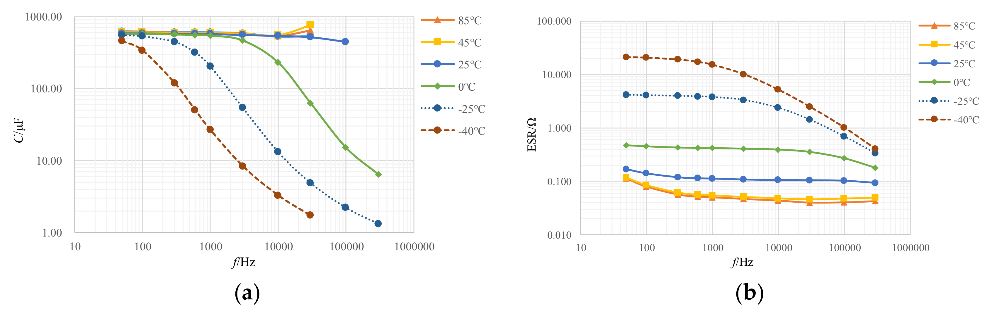
In general, C and ESR are used as the indicators of degradation AECs. However, the values of ESR and C are affected not only by aging but also temperature and frequency. Figure 1a,b show the frequency characteristic curves of C and ESR for capacitor CD297 450V680μF (Jianghai, Nantong, China) at different temperatures. The frequency characteristic curves of C and ESR are affected by the dielectric absorption and dielectric dissipation factors of AEC, which are mainly determined by the frequency characteristics of aluminum oxide film and electrolyte. From Figure 1a, it can be seen that C presents two different characteristics in high temperature zone (45~85 °C) and low temperature zone (−40~25 °C). In the high temperature zone, the capacitance increases as the frequency increases, and in the low temperature zone, the capacitance decreases as the frequency increases. Moreover, at the same frequency, the capacitance presents a non-monotonic temperature characteristic. From Figure 1b, it can be seen that the ESR-f curve has good temperature and frequency monotonicity: ESR decreases as frequency increases and decreases as temperature increases. If a converter operates at a temperature of 0~85 °C and at a frequency of 10~100 kHz, it can be found that ESR has lower temperature sensibility and lower frequency sensibility than C. Not only that, ESR also has higher degradation sensibility, which has been indicated in [7,8]. The accelerated aging test results at 120 Hz are presented in Figure 2, where it can be found that the relative variations of ESR are much larger than that of C. As a matter of fact, the evaporation of the electrolyte is the main degradation pattern of AEC. The evaporation of the electrolyte will cause an increase in ESR directly and C is mainly affected by the thickness of alumina film. In the service life of an AEC, the variation of C is not permitted beyond 20% but the variation of ESR usually exceeds 100%. Therefore, ESR is chosen as the optimum degradation parameter for AECs.

3. ESR Estimation Schemes

In power electronics converters, voltage ripples and current ripples are the basis for C and ESR calculation. Therefore, it is necessary to analyze the ripple characteristic. In general, from capacitor perspective, the output structure of power electronic converter can be illustrated as shown in Figure 3, where i_ls is the total current of the capacitor branch and load branch, i_C is the current of the capacitor branch, the electrolytic capacitor C_f is equivalent to a capacitance C in series with a resistance ESR, and R_o is the output load.

In such a structure, the output voltage ripple v_{o_ac} can be divided into two components

$$v_{\mathrm{o}\_\mathrm{ac}}=v_{\mathrm{ESR}}+v_{\mathrm{C}\_\mathrm{ac}},$$

(1)

where v_ESR and v_{C_ac} are the ripple voltages across ESR and C, respectively.

According to the characteristics of resistance and capacitance, the two components have a relationship as

$$C\frac{\mathrm{d}{v}_{\mathrm{C}\_\mathrm{ac}}}{\mathrm{d}t}=\frac{v_{\mathrm{ESR}}}{\mathrm{ESR}}=i_{\mathrm{C}},$$

(2)

If v_ESR and i_C are extracted, ESR can be calculated directly. However, in actual circuit, only v_{o_ac} (a total of v_ESR and v_{C_ac}) and i_C can be acquired. Therefore, the key of ESR estimation is the separation of v_ESR from v_{o_ac}, which can be regarded as a signal processing issue. The existing methods of signal processing can be classified into frequency-domain approaches and time-domain approaches. The frequency-domain approaches can only separate different frequency components, which are difficult to extract v_ESR from v_{o_ac} at the same frequency. For this reason, time-domain analysis is carried out in the following.

In general, the impedance of the electrolytic capacitor at the switching frequency is much less than that of the load. In this situation, almost all the switching frequency ripple current i_{ls_ac} flows through the capacitor, which can be described as

$$i_{\mathrm{C}}\approx i_{\mathrm{ls}\_\mathrm{ac}},$$

(3)

Notably, this formula is the presupposition of the proposed calculation models in this paper, which indicates that the following proposed models are applicable as long as the impedance of the load is much larger than the impedance of AEC at the switching frequency. Additionally, for the sake of analysis, resistive load is adopted for the following model derivation.

3.1. ESR Estimation Schemes Analysis

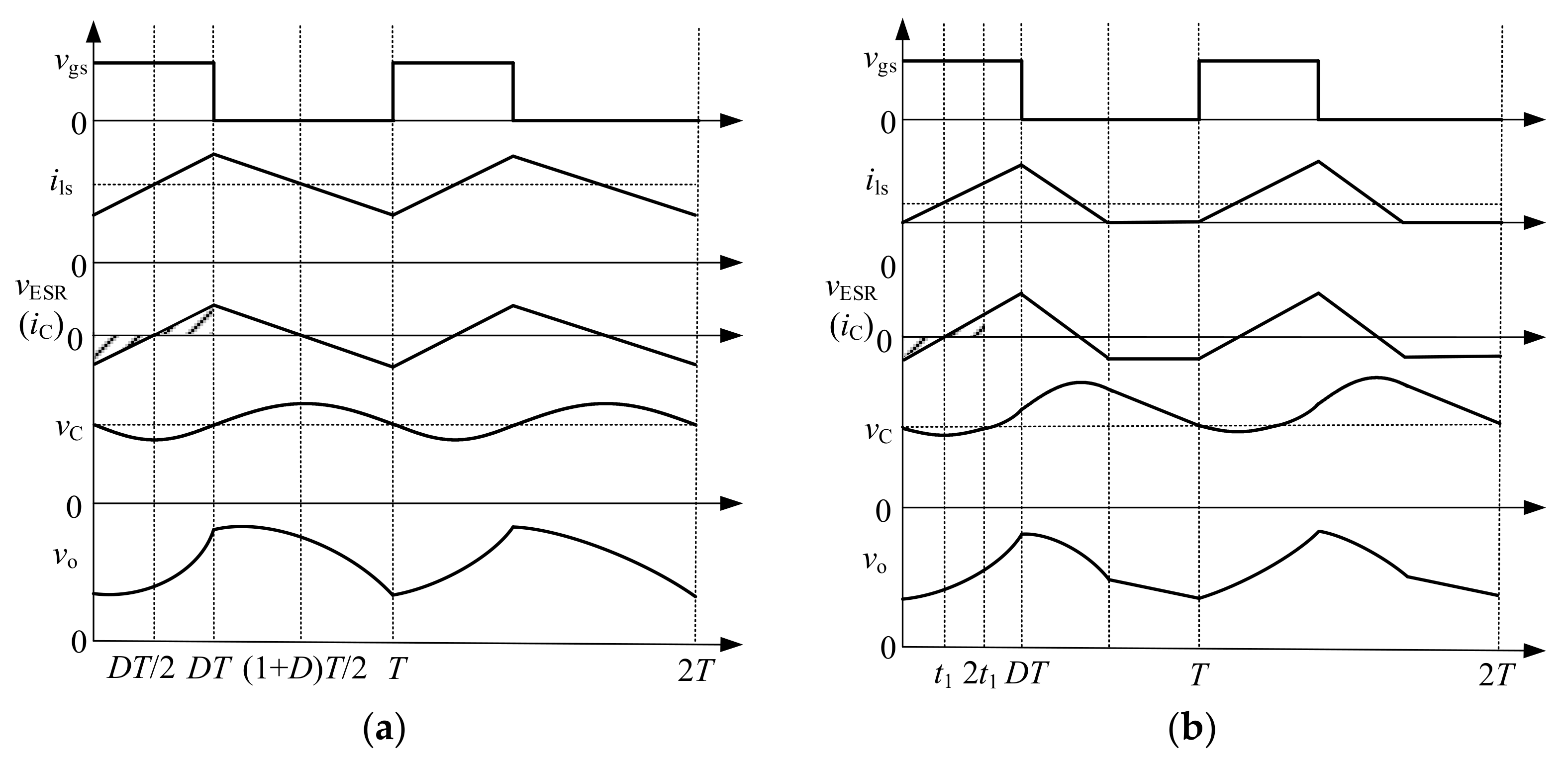
The representative waveforms of the Buck converter in CCM and DCM are shown in Figure 4a,b, respectively, where v_gs is the driving signal, v_ESR represents the voltage across the ESR (the capacitor current i_C), v_C represents the voltage across the pure capacitance, and v_o is the output voltage. From Figure 4, two characteristics can be observed: 1. there are two different moments that v_C has the same amplitude; 2. v_{C_ac} is orthogonal to v_ESR on the interval [0, T].

3.1.1. Scheme 1: Based on the Specific Moments

According to (1) and (2), ESR can be calculated by

$$\Delta v_{\mathrm{o}\_\mathrm{ac}}=\Delta v_{\mathrm{ESR}}+\Delta v_{\mathrm{C}\_\mathrm{ac}},$$

(4)

$$\mathrm{ESR}=\frac{\Delta v_{\mathrm{ESR}}}{\Delta i_{\mathrm{C}}},$$

(5)

From (4) and (5), it can be seen that ESR can be calculated by Δv_{o_ac}/Δi_C when Δv_{C_ac} = 0. Therefore, ESR can be obtained easily if the extracted two moments satisfy Δv_{C_ac} = 0. In CCM, i_C is a triangular wave and i_C(DT/2) is at the midpoint of the rising edge, namely v_C(0) = v_C(DT). In DCM, t₁ is the zero crossing point of i_C and 2t₁ is less than DT obviously. As a result, there is also a moment 2t₁ that satisfies v_C(0) = v_C(2t₁) in DCM.

In conclusion, ESR calculation model can be derived as

$$\mathrm{ESR}=\frac{v_{\mathrm{o}\_\mathrm{ac}}(0)-v_{\mathrm{o}\_\mathrm{ac}}(x)}{i_{\mathrm{C}}(0)-i_{\mathrm{C}}(x)},$$

(6)

where x = DT in CCM and x = 2t₁ in DCM.

3.1.2. Scheme 2: Based on the Orthogonality

For the reason that it only contains ac components and satisfies the Dirichlet principle, i_C(t) can be expressed in the form of Fourier as

$$i_{\mathrm{C}}(t)={\displaystyle \sum _{n=1}^{\infty }(a_{\mathrm{n}}\cos (2n\pi f_{\mathrm{s}}}t)+b_{\mathrm{n}}\sin (2n\pi f_{\mathrm{s}}t)),$$

(7)

where f_s represents the switching frequency. Substituting (7) into (2), v_{C_ac} can be obtained as

$$v_{\mathrm{C}\_\mathrm{ac}}(t)=\frac{1}{2\pi f_{\mathrm{s}}C}{\displaystyle \sum _{n=1}^{\infty }\frac{1}{n}(a_{\mathrm{n}}\sin (2n\pi f_{\mathrm{s}}}t)-b_{\mathrm{n}}\cos (2n\pi f_{\mathrm{s}}t)),$$

(8)

It can be found that

$${\displaystyle {\int }_0^T{i}_{\mathrm{C}}(t)v_{\mathrm{C}\_\mathrm{ac}}(t)dt}=\frac{1}{2\pi f_{\mathrm{s}}C}{\displaystyle \sum _{n=1}^{\infty }{\displaystyle {\int }_0^{\frac{1}{f_{\mathrm{s}}}}\frac{1}{n}\left[\begin{array}{l}\frac{a_{\mathrm{n}}^2-b_{\mathrm{n}}^2}{2}\sin (4n\pi f_{\mathrm{s}}t)\\ -a_{\mathrm{n}}{b}_{\mathrm{n}}\cos (4n\pi f_{\mathrm{s}}t)\end{array}\right]}}=0,$$

(9)

which proves the orthogonality of v_{C_ac} and v_ESR(i_C) on the interval [0, T]. Moreover, similarly, if the equivalent series inductance (ESL) is considered, the ac voltage across ESL is also orthogonal to v_ESR(i_C) on the interval [0, T], which means that the ESL of AEC does not affect the results.

Moreover, it can be further derived that

$${\displaystyle {\int }_0^T{i}_{\mathrm{C}}(t)v_{\mathrm{o}\_\mathrm{ac}}(t)dt}={\displaystyle {\int }_0^T{i}_{\mathrm{C}}(t)(v_{\mathrm{C}}(t)+v_{\mathrm{ESR}}(t))dt}={\displaystyle {\int }_0^T{i}_{\mathrm{C}}(t)(v_{\mathrm{C}}(t)+\mathrm{ESR}{i}_{\mathrm{C}}(t))dt}=\mathrm{ESR}{\displaystyle {\int }_0^T{i}_{\mathrm{C}}^2(t)dt},$$

(10)

Thus, the calculation model of ESR can be presented finally as

$$\mathrm{ESR}=\frac{{\displaystyle {\int }_0^T{i}_{\mathrm{C}}(t)v_{\mathrm{o}\_\mathrm{ac}}(t)dt}}{{\displaystyle {\int }_0^T{i}_{\mathrm{C}}^2(t)dt}},$$

(11)

The numerator of (11) is the ac loss of AEC in one switching cycle. In a power electronic converter, i_C is almost unaffected by ESR variation, which means the ac loss of AEC will increase while ESR increases and it is important to monitor the ESR variation.

3.2. ESR Estimation Implementations

Two ESR estimation schemes are revealed by (6) and (11), respectively, and there are various ways to realize them. In this part, we will provide a simple and efficient solution for each scheme.

3.2.1. Implementation of Scheme 1

In scheme 1, t₁ in DCM is difficult to obtain and i_{ls_ac} needs to be measured to capture t₁. To reduce the number of measured signals, i_C in (6) can be replaced by i_{ls_ac} as

$$\mathrm{ESR}=\frac{v_{\mathrm{o}\_\mathrm{ac}}(0)-v_{\mathrm{o}\_\mathrm{ac}}(x)}{i_{\mathrm{ls}\_\mathrm{ac}}(0)-i_{\mathrm{ls}\_\mathrm{ac}}(x)},$$

(12)

Actually, these specific moments can be obtained by capturing the zero crossing moments of v_{C_ac} and (12) can be transformed into

$$\mathrm{ESR}=\frac{v_{\mathrm{o}\_\mathrm{ac}}(t_{z1})-v_{\mathrm{o}\_\mathrm{ac}}(t_{z2})}{i_{\mathrm{ls}\_\mathrm{ac}}(t_{z1})-i_{\mathrm{ls}\_\mathrm{ac}}(t_{z2})},$$

(13)

where t_z1 and t_z2 are the two continuous zero crossing points of v_{C_ac}. t_z1 and t_z2 can be captured by extracting the zero crossing points of the integral for i_{ls_ac}. However, the integral often introduces dc components, which will lead to the extraction errors. To avoid this defect, Hilbert transform is used to replace the integral. Hilbert transform is a signal processing method that can achieve a 90-degree move-phase at all frequencies. Hilbert transform is realized by using the “hilbert” function on MATLAB, which is used to obtain the analytic signal of i_{ls_ac}:

$$hilbert(i_{\mathrm{ls}\_\mathrm{ac}})=v_{\mathrm{o}\_\mathrm{ac}}+i\times \mathrm{Hilbert}(i_{\mathrm{ls}\_\mathrm{ac}})$$

(14)

where Hilbert(i_{ls_ac}) is the actual Hilbert transform of i_{ls_ac} and is acquired by the “imag” function.

3.2.2. Implementation of Scheme 2

To implement scheme 2, the ESR calculation model of (11) can be discretized into

$$\mathrm{ESR}=\frac{{\displaystyle \sum _{i=1}^N{I}_{\mathrm{ls}\_\mathrm{ac}}(i)V_{\mathrm{o}\_\mathrm{ac}}(i)}}{{\displaystyle \sum _{i=1}^N{I}_{\mathrm{ls}\_\mathrm{ac}}^2(i)}},$$

(15)

where N is sampling number and N should cover several switching periods.

4. Simulation Study

For verifying effectiveness of the proposed ESR calculation models, the simulation model of Buck converter is built on MATLAB/SIMULINK, and the circuit parameters are listed in

Table 1. Simulation Parameters of Buck Converter.

Parameters	Variable	Value
Input voltage	Vin/V	24
Inductance	Lf/μH	220
Output capacitor	Cf/μF	100
Output load resistor	Ro/Ω	10(CCM), 100(DCM)
ESR of output capacitor	ESR/Ω	0.2
Duty cycle	D	0.5
Switching frequency	fs/kHz	50
Sampling frequency	fsa/MHz	10

. R_o = 10 Ω and R_o = 100 Ω are used for CCM simulation and DCM simulation, respectively.

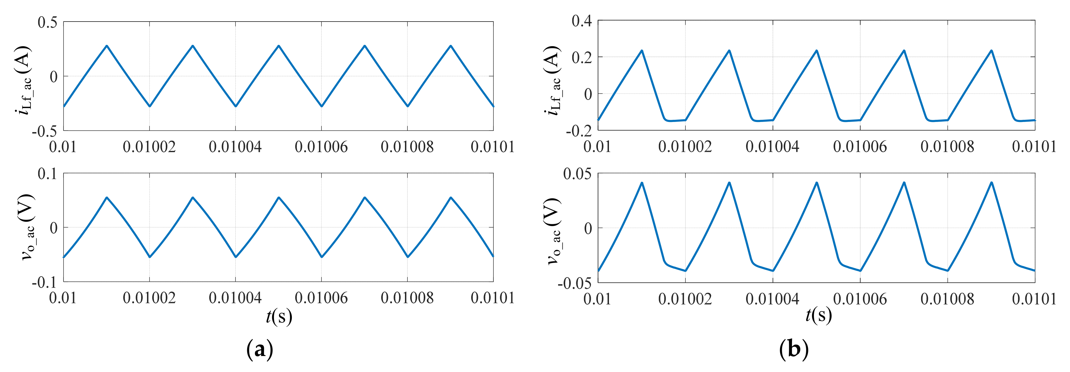
For the proposed two calculation models, the sampled signals are both the inductor ac current i_{Lf_ac} and the output ac voltage v_{o_ac}. The waveforms of i_{Lf_ac} and v_{o_ac} in CCM and DCM are shown in Figure 5, respectively.

4.1. Method 1

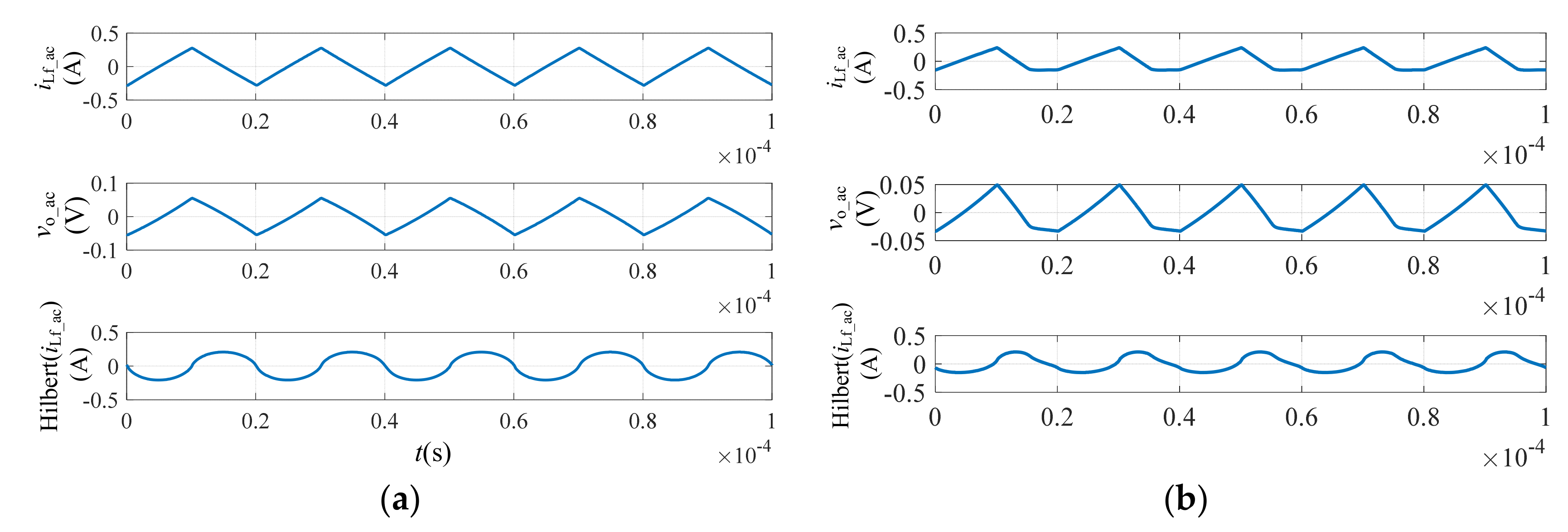
Figure 6 shows the signal processing waveforms and

Table 2. ESR Simulation Results of Buck Converter by Method 1.

Reference	Simulation Results
ESR/Ω	CCM (Ro = 10 Ω)		DCM (Ro = 100 Ω)
	ESR/Ω	error/%	ESR/Ω	error/%
0.2	0.1975	1.25	0.2020	1

lists the ESR estimation results calculated by (13) in CCM and DCM. The estimation error is about 1% and the estimation error in DCM is a little smaller than that in CCM.

The advantages of method 1 is that it only needs to capture two points for a calculation and it can reserve low computational complexity. However, it is precisely because the data used for calculation are few that this method is sensitive to noise, which means it requires high-accuracy sampling and a good de-noising method.

4.2. Method 2

Table 3. ESR Simulation Results of Buck Converter by Method 2.

Reference	Simulation Results
ESR/Ω	CCM (Ro = 10 Ω)		DCM (Ro = 100 Ω)
	ESR/Ω	error/%	ESR/Ω	error/%
0.2	0.1962	1.9	0.1999	0.05
	0.1962	1.9	0.1997	0.15
	0.1962	1.9	0.1996	0.20
	0.1962	1.9	0.1996	0.20
	0.1962	1.9	0.1996	0.20

lists the ESR estimation results calculated by (15). For each calculation, 1000 data points (five switching cycles) are acquired and ESR is calculated by 200, 400, 600, 800 and 1000 points, respectively, from top to bottom. It can be seen that the simulation results are a little smaller than the reference, whether in CCM or DCM. This is caused by the approximation of (3). In fact, some of i_{ls_ac} flows through the load resistance and the actual calculation value is ESR//R_o. For the same ESR, the larger R_o is, the smaller error is. In given R_o circumstance, the calculated results can be corrected correspondingly.

Compared to method 1, method 2 requires more data for calculation and needs more computation. However, method 2 can get a better anti-noise property for the use of more sampling data and can reduce the requirement for the sampling device.

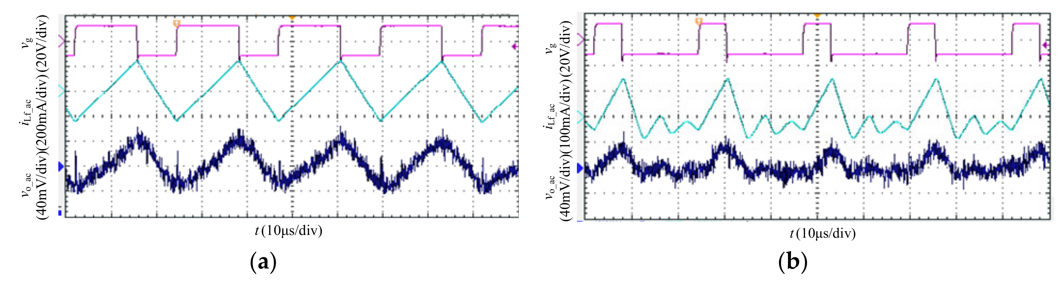
5. Experimental Results

To validate the proposed schemes, a Buck converter is assembled in the laboratory. The Buck converter is open-loop controlled and the output voltage is regulated by the duty cycle of MOSFET, which is realized by IC SG3525 (Motorala, Tokyo, Japan). The driving signal of MOSFET is produced by IC IXDN609PI (IXYS, Milpitas, CA, USA). The main specifications are as follows: input voltage: 24 V; output voltage: 12 V; switching frequency: 44.5 kHz; power diode: IXYS DSEP60-06A (IXYS, Milpitas, CA, USA); power MOSFET: IXYS IXFK64N50P (IXYS, Milpitas, CA, USA); output AEC: CAPXON 100V100μF (CapXon, Shenzhen, China); load resistance R_o: 10 Ω/400 Ω. The waveform data are acquired by Agilent DSO-X 2014a (Agilent Technologies, Santa Clara, CA, USA) and the sampling frequency is 100MHz. The collected data are uploaded to the computer and ESR is calculated on MATLAB 2016b (MathWorks, Natick, MA, USA). The reference values are measured offline by LCR meter at the switching frequency before the capacitor is assembled to the converter at 25 °C.

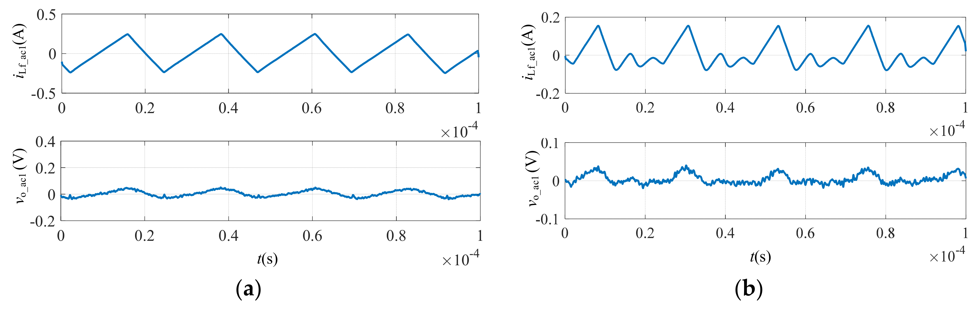
The sampled experimental waveforms are shown in Figure 7. It can be seen that the collected signals are mixed with much noise, especially v_{o_ac}, which will cause large estimation errors and even estimation failure. To eliminate the influence of noise on estimation results, a wavelet threshold de-noising method is adopted. The effect of the wavelet de-noising method mainly depends on the choice of wavelet generating function, the level of decomposition, and the setting of threshold. Synthesizing the maximum signal–noise ratio principle and calculation efficiency, Wavelet Coiflets 5 is chosen, the level of decomposition is set as 3 and fixed threshold mode is adopted. The de-noised waveforms are shown in Figure 8 and these de-noised waveforms are used for ESR estimation.

5.1. Method 1

To calculate ESR by method 1, the Hilbert transform of the inductor ac current is carried out and the waveforms of CCM and DCM are shown in Figure 9, respectively. The dotted boxes in the figure depict the zero-crossing points and the actual calculation times (5 times in CCM and 9 times in DCM). The experimental ESR estimation results of method 1 are listed in

Table 4. ESR Experimental Results of Buck Converter by Method 1 after De-noising.

Reference	Experimental Results
ESR/Ω	CCM (Ro = 10 Ω)		DCM (Ro = 400 Ω)
	ESR/Ω	error/%	ESR/Ω	error/%
0.1922	0.1733	9.8	0.1846	3.9
	0.1815	5.6	0.2133	10.9
	0.1823	5.2	0.1818	5.4
	0.1798	6.5	0.2147	11.7
	0.1855	3.5	0.1799	6.4
	-		0.2153	12.0
			0.1777	7.5
			0.2155	12.1
			0.1789	6.9

.

As the results are calculated by the data of two specific moments, the estimation results are easily affected by the noise and fluctuate obviously. From Figure 8, it can found that the signal–noise ratio of v_{o_ac1} in DCM is smaller than that in CCM, which agrees well with the higher volatility in the estimation results in DCM. By comparing the results of narrow and wide time intervals in DCM, it shows that the results in wide time intervals have higher precision and this is because the signals in wide time intervals have higher signal–noise ratio. Overall, this scheme has bad identification stability in low signal-to-noise ratio conditions and it is suitable for high-precision sampling and low-complexity computation occasions.

5.2. Method 2

The experimental results of method 2 are listed in

Table 5. ESR Experimental Results of Buck Converter by Method 2 after De-noising.

Reference	Experimental Results
ESR/Ω	CCM (Ro = 10 Ω)		DCM (Ro = 400 Ω)
	ESR/Ω	error/%	ESR/Ω	error/%
0.1922	0.1819	5.3	0.1994	3.7
	0.1813	5.7	0.2004	4.3
	0.1763	8.3	0.1882	2.1
	0.1767	8.1	0.1878	2.3

. ESR is calculated with one cycle (N = 2247) to eight cycles (N = 8988). In comparison with the results of CCM, the results in DCM are closer to the reference. This is caused by the approximation of (3), which agrees well with the simulation. Moreover, the cross correlation coefficient of the noise is usually very small, which means this method has good noise immunity. To verify the noise immunity, ESR estimation results calculated by using the signals before de-noising are listed in

Table 6. ESR Experimental Results of Buck Converter by Method 2 before De-noising.

Reference	Experimental Results
ESR/Ω	CCM (Ro = 10 Ω)		DCM (Ro = 400 Ω)
	ESR/Ω	error/%	ESR/Ω	error/%
0.1922	0.1810	5.8	0.1917	0.3
	0.1802	6.2	0.2002	4.2
	0.1751	8.9	0.1879	2.2
	0.1755	8.7	0.1875	2.4

. Compared to the results in Table 5, the difference of the results in Table 6 is small, which verifies the good noise immunity of this method. Overall, this scheme has good identification precision and stability.

5.3. Error Analysis

In addition to the load resistance, the estimation error of the proposed methods is also induced by other factors:

• Noise effect. Though the signal-to-noise ratio is greatly improved by the wavelet de-noising method, noise cannot be completely eliminated and the effective signal is also attenuated.
• Sampling resolution. The estimation precision is determined by the sampling resolution of voltage and current ripples. However, the voltage and current ripples are small, which needs equipment with high resolution.
• Errors of the reference values. Errors also exist in the measured reference values and only values at a certain frequency can be measured by LCR meter. However, the used inductor current and capacitor voltage for ESR estimation not only contain switching-frequency components, but also an amount of harmonic components, which will lead to different estimation results.
• The delay mismatching of the voltage sensor and current sensor. The ESR estimation method is based on the phase relationship and the different delay time of voltage and current sensors will result in errors. In this respect, the delay time difference should be minimized so as to achieve high accuracy.

Although there are some errors in the estimation results, the results have low dispersed degree. The aim of ESR estimation is to monitor the health of AEC, which is often considered lapsed until its ESR increases to more than two times of the initial value. Therefore, the estimation error (<10%) is within the accepted range and the estimation results can be taken as effective indicators.

6. Conclusions

From a capacitor perspective, ESR calculation schemes of output capacitors for a Buck converter are studied in this paper:

(1)

The degradation parameters of AECs are analyzed and ESR is indicated as the optimal health indicator.

(2)

Based on the voltage–current characteristics, two ESR calculation models are proposed.

To reveal the advantages of the proposed methods, a comparison between the two proposed methods and the existing methods is presented in

Table 7. Comparison between the Proposed Methods and the Existing Methods.

Method	The Existing Capacitor Perspective Methods (CPMs)	Proposed Method 1	Proposed Method 2
Calculation model	simple	simple	simple
Additional circuit	relatively complicated	simple	simple
Load applicability	CCM or DCM	Both CCM and DCM	Both CCM and DCM
Applicability	narrow	wide	wide

.

The main advantages of the two proposed methods are:

(1)

Only the output voltage ripple and the inductor current ripple are sampled, which requires minimal hardware.

(2)

The proposed methods apply to both CCM and DCM.

The main differences between method 1 and method 2 are:

(1)

Method 1 only needs to capture two points for calculation in a switching period and method 2 needs to continuously capture several switching-period points.

(2)

Method 1 is susceptive to noise and method 2 has a strong capability for noise immunity.

It should be noted that the proposed methods are only applicable to the case that the output is a single capacitor or the case that the output can be equivalent to a single capacitor. The proposed methods are not effective and need to be improved for parallel capacitors. Ultimately, we are still working on the optimal method of monitoring parallel capacitors.