Real-time Neural Networks Implementation Proposal for Microcontrollers

Abstract

The adoption of intelligent systems with Artificial Neural Networks (ANNs) embedded in hardware for real-time applications currently faces a growing demand in fields such as the Internet of Things (IoT) and Machine to Machine (M2M). However, the application of ANNs in this type of system poses a significant challenge due to the high computational power required to process its basic operations. This paper aims to show an implementation strategy of a Multilayer Perceptron (MLP)-type neural network, in a microcontroller (a low-cost, low-power platform). A modular matrix-based MLP with the full classification process was implemented as was the backpropagation training in the microcontroller. The testing and validation were performed through Hardware-In-the-Loop (HIL) of the Mean Squared Error (MSE) of the training process, classification results, and the processing time of each implementation module. The results revealed a linear relationship between the values of the hyperparameters and the processing time required for classification, also the processing time concurs with the required time for many applications in the fields mentioned above. These findings show that this implementation strategy and this platform can be applied successfully in real-time applications that require the capabilities of ANNs.

1. Introduction

Microcontrollers ($\mathsf{\mu }$Cs) have been applied in many areas: industrial automation, control, instrumentation, consumer electronics, and various other areas. Nonetheless, there is an ever-growing demand for these devices, especially in emerging sectors such as the Internet of Things (IoT), the smart grid, Machine to Machine (M2M), and edge computing [1].

A $\mathsf{\mu }$C can be classified as programmable hardware platform that enables embedded system applications in specific cases. It is important to know that $\mathsf{\mu }$Cs are mainly composed of a General-Purpose Processor (GPP) of 8, 16, or 32 bits. Then, this GPP is connected to some peripherals such as Random Access Memory (RAM), flash memory, counters, signal generators, communication protocol specific hardware, analog-to-digital and digital-to-analog converters, and others.

An important fact is that in most products that are available today, the $\mathsf{\mu }$Cs embedded into them encapsulate an 8-bit GPP with enough computational power and memory storage for use as a resourceful platform for many embedded applications. However, these same 8-bit $\mathsf{\mu }$Cs are considered low-power and low-cost platforms when compared with other platforms that are used to implement AI applications with Artificial Neural Networks (ANNs) [2,3].

The use of artificial intelligence algorithms, such as (ANN, Fuzzy, SVM, Genetic Algorithms, and other ) for embedded systems with real-time constraints, has been a recurrent research topic for many [4,5,6,7,8,9,10,11,12,13,14]. Many of the works devised from this topic are driven by the growing demand for AI techniques for IoT, M2M, and edge computing applications.

A major problem with implementing ANN applications into embedded systems is the computational complexity associated with ANNs. In regard to the Multilayer Perceptron (MLP) described in this work, there are many inherent multiplications and calculations of nonlinear functions [4,5,6]. Besides the feedforward process between the input and the synaptic weights, the MLP also has a training algorithm associated with it to find the optimum weights of the neural network. This training algorithm is very computationally expensive [15]. If the training process is also performed in real time, the computational complexity is increased several times. This increase in complexity automatically raises the processing time and requirements for memory storage from the hardware platform used in the application [4,5,6].

The use of MLP neural networks for real-time applications in $\mathsf{\mu }$Cs is not a new field. In [16], the authors describe a method to linearize the nonlinear characteristics of many sensors using an MLP-NN on an 8-bit PIC18F45J10 $\mathsf{\mu }$C. The obtained results show that if the network architecture is right, even very difficult problems of linearization can be solved with just a few neurons.

In [17], a fully connected multilayer ANN is implemented on a low-end and inexpensive $\mathsf{\mu }$C. Furthermore, a pseudo-floating-point multiplication is devised to make use of the internal multiplier circuit inside the PIC18F45J10 $\mathsf{\mu }$C used. The authors managed to store 256 weights into the 1KB SRAM of the $\mathsf{\mu }$C and deemed it enough for most embedded applications.

In [18], Farooq et al. implemented a hurdle-avoidance system controller for a carlike robot using an AT89C52 $\mathsf{\mu }$C as a system embedding platform. They implemented an MLP with a back-propagation training algorithm and a single hidden layer. The proposed system was tested in various environments containing obstacles and was found to avoid obstacles successfully.

The paper [19] presents a neural network that is trained with the backpropagation (BP) algorithm and validated using a low-end and inexpensive PIC16F876A 8-bit $\mathsf{\mu }$C. The authors chose a chemical process as a realistic example of a nonlinear system to demonstrate the feasibility and performance of this approach, as well as the results found using the microcontroller, against a computer implementation. With three inputs, five hidden neurons, and an output neuron on the MLP, the application showed complete suitability for a $\mathsf{\mu }$C-based approach. The results comparing the $\mathsf{\mu }$C implementation showed almost no difference in Mean Square Error (MSE) after 30 iterations of the training algorithm. The work presented in [20] shows an embedded MLP with two layers on the microcontroller. The proposal uses an external tool for training and embedding a trained ANN.

In [21], the authors implemented a classification application for the MNIST dataset. This implementation processes the 10 digits and full classification with $99.15\%$ testing accuracy. In addition, this is implemented with a knowingly highly resource-hungry ANN model, the Convolutional Neural Network (CNN), using less than 2 KB of SRAM memory and also 6 KB of program memory, FLASH. This work was embedded on a Arduino Uno development kit that is composed of a breakout board for the 8-bit ATMega328p $\mathsf{\mu }$C, with 32 KB of program memory and 2 KB of work memory, running at 16 MHz.

In [22], the authors present an approach of reordering the operations on an ANN, reducing the memory usage for a CNN. They deployed a SwiftNet Cell with 250 KB of parameters into a Cortex-M7, 32-bit $\mathsf{\mu }$C, running at 216 MHz, with 512 KB of SRAM. The results of reordering the operations showed an increase in inference time and energy use of less than 1% and a decrease of approximately 53% of peak memory usage, thus showing that such applications can be made in 32-bit $\mathsf{\mu }$Cs.

The reference works presented above demonstrate different aspects of implementing ANNs on $\mathsf{\mu }$Cs. In [17,18,19], you will find application proposals showing MLP-ANNs trained with the backpropagation (BP) algorithm implemented on $\mathsf{\mu }$Cs with good results; however, none of these talk about memory usage and processing-time parameters that vary according to the MLP hyperparameters. In [16,23,24], the authors present some results regarding processing time, but none are dependent on the number of artificial neurons or even comparing the time required to train the ANN in real time or not.

Therefore, this work proposes an implementation of an MLP-ANN that can be trained with the BP algorithm into an ATMega2560 8-bit $\mathsf{\mu }$C in the C language to show that many applications with ANNs are suitable on the $\mathsf{\mu }$C platform. This work also presents two implementations regarding a model that is trained on the $\mathsf{\mu }$C platform in real time and another implementation that is trained with MatLab and then ported to the same architecture to execute classification in real time.

In addition to the implementation proposal, the parameters of the processing time for each feedforward step and backward steps in the training and classification process are presented. In addition, the variation of these parameters is shown due to the variation of the hyperparameters of the MLP. The validation of the classification and training results on a Hardware-In-the-Loop (HIL) strategy also are presented in this work.

2. System Description

Figure 1 shows a block diagram detailing the modules implemented into the $\mathsf{\mu }$C. This implementation has the work in [25] as a direct reference, which models the MLP as a matrix form, simplifying and modularizing all the feedforward and backwards propagation.

As seen in Figure 1, the structure of the MLP here implemented has four main modules: the Input Random Permutation Module (IRPM), the FeedForward Module (FFM-k), the Error Module (EM), and the Backpropagation Module (BPM-k), in which the variable k represents the ANN layer. It is important to add that the implementation presented in this work is shown with two layers (one hidden and the output layer), but it can be easily extended for more if required. The modules and associated mathematical modeling will be detailed in the following subsections.

2.1. Associated Variables

The implementation is composed of four main variables that are passed by reference between the modules. These variables are the input signals matrix, ${\mathbf{Y}}^{k=0}\left(n\right)$ defined as

$${\mathbf{Y}}^0\left(n\right)=\left[{\mathbf{y}}_1^0\left(n\right),\dots ,{\mathbf{y}}_s^0\left(n\right),\dots ,{\mathbf{y}}_{\mathbb{N}}^0\left(n\right)\right],$$

(1)

where $k=0$ means that this matrix is dealing with the input layer of the MLP, n represents the iteration number of the training algorithm. $\mathbb{N}$ is defined as the number of samples of a training set and ${\mathbf{y}}_s$ the s-th sample defined as

$${\mathbf{y}}_s^0\left(n\right)={\left[y_{s1}^0\left(n\right),\dots ,y_s^0\left(n\right),\dots ,y_P^0\left(n\right)\right]}^T,$$

(2)

where P is the number of available inputs of the MLP. The synaptic weights matrix from the k-th layer, ${\mathbf{W}}^k\left(n\right)$, is defined as

$${\mathbf{W}}^k\left(n\right)=\left[\begin{array}{ccccc}{w}_{10}^k\left(n\right)& \cdots & w_{1h}^k\left(n\right)& \cdots & w_{1H^{k-1}}^k\left(n\right)\\ ⋮& \ddots & ⋮& \ddots & ⋮\\ w_{j0}^k\left(n\right)& \cdots & w_{jh}^k\left(n\right)& \cdots & w_{j{H}^{k-1}}^k\left(n\right)\\ ⋮& \ddots & ⋮& \ddots & ⋮\\ w_{H^{k}0}^k\left(n\right)& \cdots & w_{H^{k}h}^{\left(y\right)}\left(n\right)& \cdots & w_{H^k{H}^{k-1}}^k\left(n\right)\end{array}\right],$$

(3)

where $H^k$ is the number of neurons from the k-th layer and $w_{ij}^k\left(n\right)$ represents the synaptic weight associated with the i-th artificial neuron, from the j-th input signal of the k-th layer at the n-th iteration. The output signals matrix, ${\mathbf{Y}}^L\left(n\right)$, is defined as

$${\mathbf{Y}}^L\left(n\right)=\left[{\mathbf{y}}_1^L\left(n\right),\dots ,{\mathbf{y}}_s^L\left(n\right),\dots ,{\mathbf{y}}_{\mathbb{N}}^L\left(n\right)\right],$$

(4)

where L is the number of layers of the MLP and also defines which layer is last, and $y_s^L\left(n\right)$ represents the output signal associated with the s-th sample input $y_s^0$ that is defined as

$${\mathbf{y}}_s^L\left(n\right)={\left[y_1^L\left(n\right),\dots ,y_s^L\left(n\right),\dots ,y_M^L\left(n\right)\right]}^T,$$

(5)

where M is the number of output neurons.

The $\mathbf{D}\left(n\right)$ variable represents the desired values or labels of the training set composed of the $\mathbf{D}\left(n\right)$ and the ${\mathbf{Y}}^0\left(n\right)$, which is defined as

$$\mathbf{D}\left(n\right)=\left[{\mathbf{d}}_1\left(n\right),{\mathbf{d}}_2\left(n\right),\dots ,{\mathbf{d}}_s\left(n\right),\dots ,{\mathbf{d}}_{\mathbb{N}}\left(n\right)\right],$$

(6)

where ${\mathbf{d}}_s\left(n\right)$ is the vector of desired values referring to the s-th sample associated with the $y_s^0\left(n\right)$ input signal, which is defined as

$${\mathbf{d}}_s\left(n\right)={\left[d_1\left(n\right),\dots ,d_s\left(n\right),\dots ,d_M\left(n\right)\right]}^T.$$

(7)

For an MLP with two layers, ${\mathbf{W}}^1\left(n\right)$ represents the synaptic weights matrix from the hidden layer ($H^0=P$), and ${\mathbf{W}}^2\left(n\right)$ is the weights matrix from the output layer ($H^2=M$) at the n-th iteration. In addition to these two matrices, a few others are created to accommodate intermediary results from feedforward and backward propagation operations of the MLP.

2.2. Feedforward Module—(FFM-k)

This module is responsible for running the feedforward operation of an MLP, propagating the inputs through each k-th layer during each n-th iteration. As with most BP implementations, this proposal can operate in online mode or batch mode (defining $\mathbb{N}>1$). At each k-th FFM-k on each k-th layer the following equation is calculated as

$${\mathbf{Y}}^k\left(n\right)=\phi \left({\mathbf{W}}^k\left(n\right){\mathbf{Y}}^{k-1}\left(n\right)\right),$$

(8)

where ${\mathbf{Y}}^{k-1}\left(n\right)$ is the output signals matrix from the previous layer. The ${\mathbf{Y}}^k\left(n\right)$ represents the output of the current layer and $\phi \left(·\right)$ is the activation function of the current k-th layer. As previously said, a few other matrices are devised as part of the BP calculation and some of them store the calculation results from Equation (8).

Algorithm 1 describes the pseudocode executed when the FFM-k module is called. The function prodMatrix() implements the matrix product between ${\mathbf{W}}^k\left(n\right)$ and ${\mathbf{Y}}^{k-1}\left(n\right)$, and in the end, it stores the product result in ${\mathbf{Y}}^k\left(n\right)$. The actFun() function executes the activation function of the k-th layer to each element of ${\mathbf{Y}}^k\left(n\right)$ and stores the result in itself (${\mathbf{Y}}^k\left(n\right)$) as it runs.

Algorithm 1 Description of the algorithm implemented by the FeedForward Module (FFM)-k module.

1: function$\mathrm{FFM}-k$(${\mathbf{W}}^k\left(n\right)$, ${\mathbf{Y}}^{k-1}\left(n\right)$, ${\mathbf{Y}}^k\left(n\right)$) 2:   $\mathrm{prodMat}\left({\mathbf{W}}^k\left(n\right),{\mathbf{Y}}^{k-1}\left(n\right),{\mathbf{Y}}^k\left(n\right)\right)$ 3:   $\mathrm{activfun}\left({\mathbf{Y}}^k\left(n\right)\right)$ 4: end function

2.3. Error Module—(EM-k)

The error module EM-k calculates the error between the desired values matrix $\mathbf{D}\left(n\right)$ and the output signals matrix ${\mathbf{Y}}^L\left(n\right)$ of the last layer, L. The equation that is evaluated at the EM-k is defined as

$$\mathbf{E}\left(n\right)=\mathbf{D}\left(n\right)-{\mathbf{Y}}^L\left(n\right).$$

(9)

Algorithm 2 describes how the EM-k module functions, in which the difMatrix() function implements the element-by-element difference between $\mathbf{D}\left(n\right)$ and ${\mathbf{Y}}^L\left(n\right)$ and stores the result into the $\mathbf{E}\left(n\right)$ matrix.

Algorithm 2 Pseudocode implementation of the Error Module (EM) module.

1: functionEM(${\mathbf{Y}}^L\left(n\right)$, $\mathbf{D}\left(n\right)$, $\mathbf{E}\left(n\right)$) 2:   $\mathrm{difMatrix}\left({\mathbf{Y}}^L\left(n\right),\mathbf{D}\left(n\right),\mathbf{E}\left(n\right)\right)$ 3: end function

2.4. Backpropagation Module—(BPM-k)

The last module is responsible for the main training part of the implementation. The BPM-k calculates the new updated values of the synaptic weights matrices of the L layers that better approximate the desired values, ${\mathbf{W}}^k\left(n\right)$. The equation that the BPM-k implements is defined as

$${\mathbf{W}}^{\left(k\right)}\left(n+1\right)={\mathbf{W}}^{\left(k\right)}\left(n\right)+\Delta {\mathbf{W}}^{\left(k\right)}\left(n\right),$$

(10)

where

$$\Delta {\mathbf{W}}^{\left(k\right)}\left(n\right)=\frac{\eta }{\mathbb{N}}{\mathbf{g}}^k\left(n\right){\left[\begin{array}{c}-\mathbf{1}\\ {\mathbf{Y}}^{k-1}\left(n\right)\end{array}\right]}^T+\alpha \Delta {\mathbf{W}}^{\left(k\right)}\left(n-1\right),$$

(11)

where $\eta$ is the learning-rate of the BP algorithm, $\alpha$ is the learning-moment rate factor, and ${\mathbf{g}}^k\left(n\right)$ is defined as

$${\mathbf{g}}^k\left(n\right)=\left\{\begin{array}{cc}\mathrm{prod}\left({\phi }^{\prime }\left({\mathbf{Y}}^k\left(n\right)\right),\mathbf{E}\left(n\right)\right)\hfill & \mathrm{for}k=L\hfill \\ {\mathbf{z}}^k\left(n\right)\hfill & \mathrm{for}1\le k<L\hfill \end{array},\right.$$

(12)

where

$${\mathbf{z}}^k\left(n\right)=\mathrm{prod}\left({\phi }^{\prime }\left(\left[\begin{array}{c}-\mathbf{1}\\ {\mathbf{Y}}^k\left(n\right)\end{array}\right]\right),{\left[{\mathbf{W}}^{\left(y\right)}\left(n\right)\right]}^T{\mathbf{g}}^{\left(k+1\right)}\left(n\right)\right)$$

(13)

and

$${\mathbf{z}}^k\left(n\right)=\left[\begin{array}{c}\begin{array}{cccc}{z}_{11}^{\left(k\right)}\left(n\right)& z_{12}^{\left(k\right)}\left(n\right)& \dots & z_{1\mathbb{N}}^{\left(k\right)}\left(n\right)\end{array}\\ {\mathbf{z}}^{\left(k\right)}\left(n\right)\end{array}\right].$$

(14)

The prod() function in Equation (13) implements an element-wise product between two matrices, implemented in Algorithm 3, and ${\phi }^{\prime }(·)$ is the derivative of the activation function.

Algorithm 3 Matrix product implementation pseudocode.

1: function$prodMat$(${\mathbf{W}}^{\mathbf{k}},{\mathbf{Y}}^{\mathbf{k}-\mathbf{1}},{\mathbf{Y}}^{\mathbf{k}},P,M,\mathbb{N}$) 2:   Initialize (i, j, s, accumulate) ← 0 3:   for i← 1 to M do 4:     for j← 1 to $\mathbb{N}$ do 5:       accumulate ← 0 6:       for s← 1 to P do 7:         accumulate = accumulate + ${\mathbf{W}}^{\mathbf{k}}$[i][s] ×${\mathbf{Y}}^{\mathbf{k}-\mathbf{1}}$[s][j] 8:       end for 9:       ${\mathbf{Y}}^{\mathbf{k}}$[i][j] = accumulate 10:     end for 11:   end for 12: end function

2.5. Basic Operations

This section describes the implementation of the basic operations used in this work. First, Algorithm 3 implements the matrix product. A very important detail is that all the modules were implemented following pointer arithmetic procedures. With this in mind, the source code is very well optimized for memory usage, reducing the overall duration of execution from each module. Every matrix used in this implementation is floating-point (IEEE754) [26] representation values.

Algorithm 4 shows the pseudocode of an element-wise product between two matrices used in this work, more specifically in the BPM-k module implementation. This same pseudocode in Algorithm 4 can be slightly altered to perform subtraction or addition by editing the operation between matrices on line 5. It is important to notice that Algorithm 4 requires that both matrices have the same dimensions.

Algorithm 4 Element-wise matrix product implementation algorithm.

1: function$prod$(${\mathbf{Y}}^{\mathbf{k}},\mathbf{E},{\mathbf{g}}^{\mathbf{k}},P,M$) 2:   Initialise (i, j) ← 0 3:   for i← 1 to P do 4:     for j← 1 to M do 5:       ${\mathbf{g}}^{\mathbf{k}}$[i][j] = ${\mathbf{Y}}^{\mathbf{k}}$[i][j] ×$\mathbf{E}$[i][j] 6:     end for 7:   end for 8: end function

Algorithm 5 presents to us the implementation of the calculation of the Trace and Product between two matrices at a single operation inside a nested loop. This simple optimization saved a few $\mathsf{\mu }$s of processing time for the overall training process.

Algorithm 6 shows the implemented steps for calculating the activation function of the induced-local-field of each neuron, an element-wise operation. This Algorithm 6 is implementing a sigmoid activation function.

Algorithm 5 Pseudocode implementation of the trace of the product between two matrices.

1: function$trace$(${\mathbf{E}}^{\mathbf{k}},{\mathbf{E}}^{\mathbf{kT}},P,M$) 2:   Initialize (i, j, trace) ← 0 3:   for i← 1 to P do 4:     for j← 1 to M do 5:       trace = trace + ${\mathbf{E}}^{\mathbf{k}}$[i][j]×${\mathbf{E}}^{\mathbf{k}}\mathbf{T}$[i][j] 6:     end for 7:   end for 8: end function

Algorithm 6 Pseudocode implementation of the sigmoid activation function.

1: function$activfun$(${\mathbf{Y}}^{\mathbf{k}},{\mathbf{Y}}^{\mathbf{k}+\mathbf{1}},P,M$) 2:   Initialise (i, j) ← 0 3:   for i← 1 to P do 4:     for j← 1 to M do 5:       ${\mathbf{y}}^{\mathbf{k}+\mathbf{1}}$[i][j] = (1.0)/(1.0 + exponential($-{\mathbf{Y}}^{\mathbf{k}}$[i][j])) 6:     end for 7:   end for 8: end function

3. Methodology

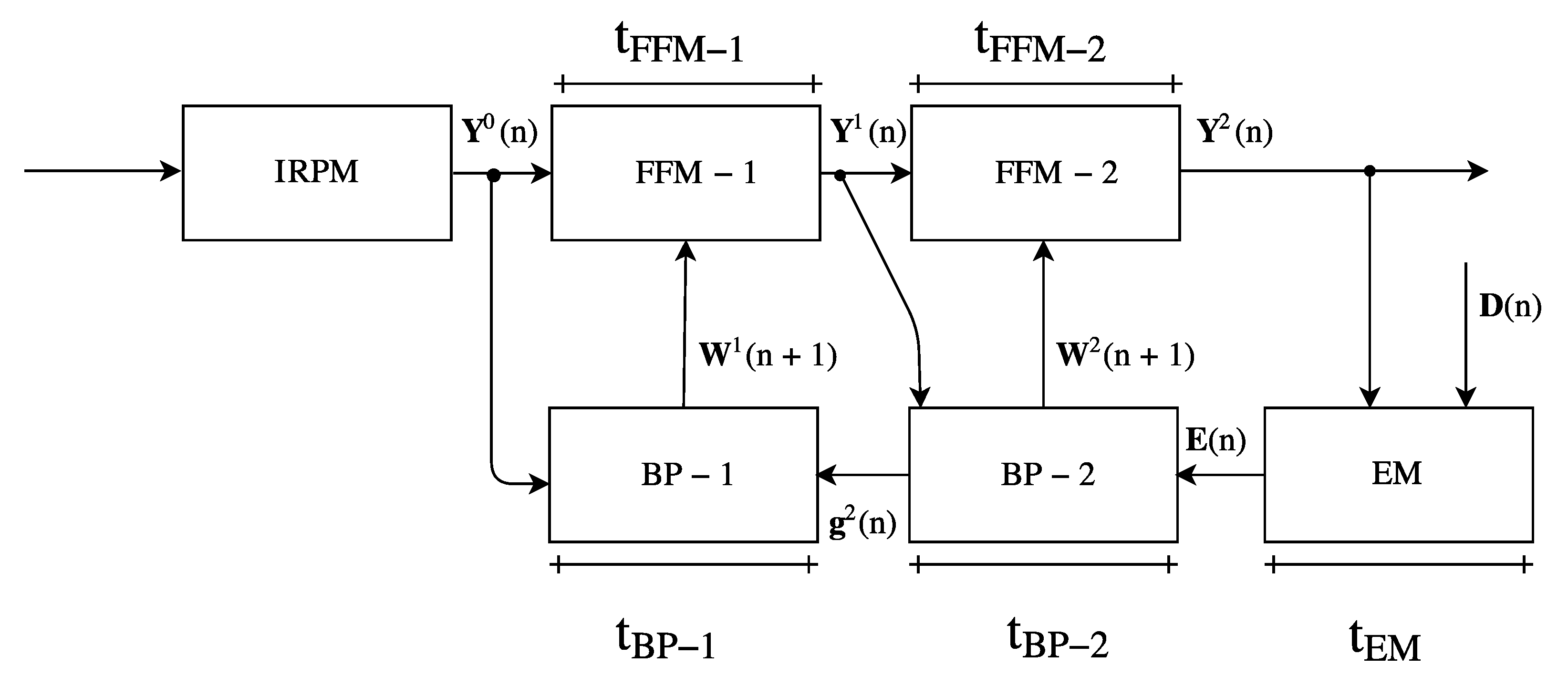
The implementation was validated using the HIL simulation strategy, as explained in [3] and illustrated in Figure 2. The tested variables are execution time for the FFM-1 for the hidden layer as seen in Figure 1 defined as $t_{\mathrm{FFM}-1}$, execution time for the FFM-2, feedforward for the output layer of neurons, $t_{\mathrm{FFM}-2}$, error module $t_{\mathrm{EM}}$, backpropagation of the output neurons layer, $t_{\mathrm{BPM}-1}$, and the backpropagation of the hidden neurons layer, $t_{\mathrm{BPM}-2}$.

A parameter that was also analyzed is the memory occupation, regarding both memories of the ATMega-2560 $\mathsf{\mu }$C used in this paper, FLASH or program memory and SRAM or work memory.

As previously mentioned, the modules were implemented in the C program language for AVR $\mathsf{\mu }$Cs using the avr-gcc version 5.4.0, inside the Atmel Studio 7 development environment, an Integrated Development Environment (IDE) made available by Microchip. After compilation and binary code generation, the solution was embedded into an Atmega-2560. This $\mathsf{\mu }$C has an 8-bit GPP integrated with 256 KBytes of FLASH program memory and 8 KBytes of SRAM work memory, and its maximum processing speed is 1 MIPS/MHz.

The Atmega-2560 is associated with an Arduino Mega v2.0 development kit: the Arduino Mega is a development kit that provides a breakout board for all the ATmega-2560 pins and some other components required for the $\mathsf{\mu }$C to function properly. A great feature of this development kit is the onboard Universal Serial Bus (USB) programmer that enables the developer to simply connect a USB port to a computer and test various implementations easily on the $\mathsf{\mu }$C.

This work was validated using two cases. First, the MLP-BP was trained to behave as an XOR operation as the simplest case possible to train an MLP and evaluate its ability to learn a nonlinear relationship between two inputs. Secondly, the network was trained to aid a carlike virtual robot in avoiding obstacles in a virtual map using MatLab and three cases of increasing ANN architecture complexity. The assembly and analysis of these two validation cases are presented in the following subsections.

3.1. Hardware-In-the-Loop Simulation

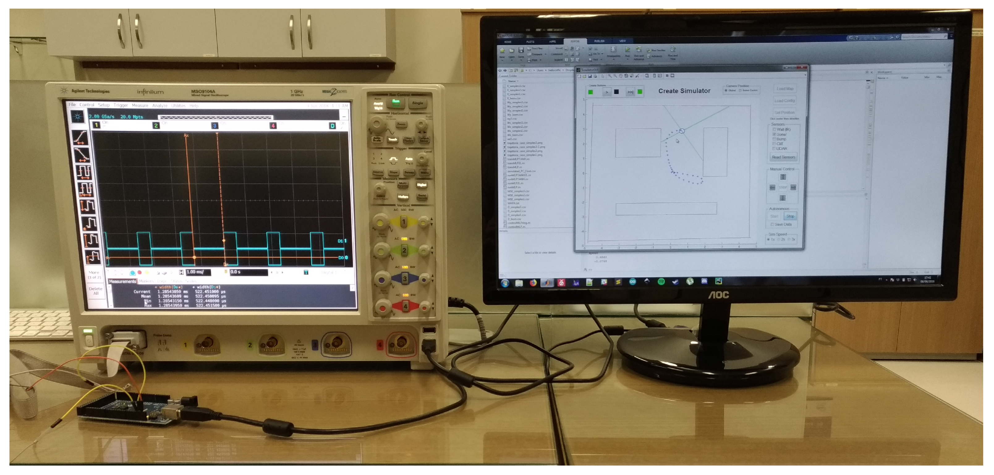
The tests were executed with the $\mathsf{\mu }$C running at a clock of 16 MHz. The results were obtained by setting the level of a digital pin of the ATMega-2560 to HIGH, executing one of the modules and setting the same digital pin logical value to LOW, and measuring the time of logic HIGH on an oscilloscope for this digital pin. This can be easily seen on Figure 2, and a picture of the HIL assembly is shown in Figure 3. Figure 4 gives a closer look at the oscilloscope measurements, taking into account all the modules being measured according to their duration of execution for the XOR validation case described below.

The calculation of the MSE during training was also embedded into the $\mathsf{\mu }$C implementation and they were transmitted through Universal Serial Synchronous Asynchronous Receiver Transmitter (USART) protocol to a computer. The calculation of the MSE is defined as

$$MSE\left(n\right)=\frac{1}{2N}\mathrm{trace}\left(\mathbf{E}{\left(n\right)}^T\mathbf{E}\left(n\right)\right),$$

(15)

where $\mathrm{trace}(·)$ is the implementation seen in Algorithm 5.

3.2. XOR Operation

A validation of the real-time embedded training using the $\mathrm{BPM}-k$ module was devised for a XOR operation, as described in

Table 1. Truth table for the XOR operation.

Input A	Input B	Result
0	0	0
0	1	1
1	0	1
1	1	0

, the most basic MLP validation case. This test was performed with training and classification phases, both running in the $\mathsf{\mu }$C, considering a configuration as seen in Figure 1. The test was executed on batch mode with $\mathbb{N}=4$, two layers of neurons ($L=2$), two input signals ($P=H^0=2$), a varying amount of neurons in the hidden neurons layer ($H^1$), and a single neuron in the output layer ($H^2=1$). It is important to notice that the strategy herein presented can be assembled with various different configurations only modifying the $P,H^k$ and M parameters, with the $\mathsf{\mu }$Cs internal memories being the limiting factor for the ANN architecture size.

3.3. Virtual Carlike Robot

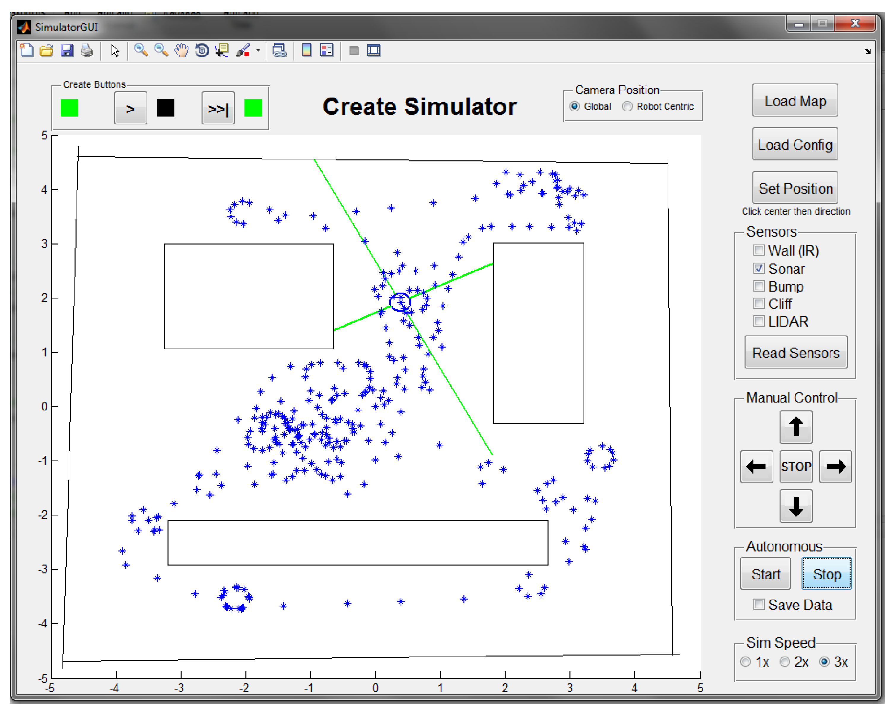
This work also tested an MLP-BP model to control a virtual carlike robot from the iRobot MatLab toolbox, provided by the United States Naval Academy (USNA) [27]. This toolbox provides a virtual environment and an interface to test control algorithms on a deferentially steered robot on various maps with different obstacles and different combinations of distance or proximity sensors.

As previously stated, this virtual environment provides an interface to control a deferentially steered virtual robot. This robot is controlled by changing the angular speed in rad/s of the two wheels, Right Wheel (RW) and Left Wheel (LW). Furthermore, this work used three proximity sensors with a virtual 3 m range to provide input to the MLP. The sensors are Front-Sensor (FS), Left-Sensor (LS) and Right-Sensor (RS).

The MLP model with three different datasets was tested, increasing the hyperparameters to evaluate the behavior of the robot. The cases are composed of three tables with five columns each, as seen in

Table 2. Training dataset for the first and simplest case. With $H^0=3$, $H^1=5$ and $H^2=2$.

Condition	FS (m)	RS (m)	LS (m)	LW (rad/s)	RW (rad/s)
1	0.00	0.00	0.00	0.50	−0.50
2	0.00	0.00	1.00	−0.50	0.50
3	0.00	1.00	0.00	0.50	−0.50
4	0.00	1.00	1.00	0.50	−0.50
5	1.00	0.00	0.00	0.50	0.50
6	1.00	0.00	1.00	0.50	0.50
7	1.00	1.00	0.00	0.50	0.50
8	1.00	1.00	1.00	0.50	0.50

. The first case is very simple with only eight conditions provided to train the network, which means the network must be able to devise a knowledge representation of how to behave with cases not previously trained from these simple constraints.

The second case has a greater complexity with 18 conditions, as seen in

Table 3. Training dataset for the second case. With $H^0=3$, $H^1=5$ and $H^2=2$.

Condition	FS (m)	RS (m)	LS (m)	LW (rad/s)	RW (rad/s)
1	0.00	0.00	0.00	−0.20	0.20
2	1.00	0.00	0.00	−0.20	0.20
3	2.00	0.00	1.00	−0.20	0.20
4	0.00	1.00	1.00	0.10	0.10
5	1.00	1.00	2.00	0.20	−0.10
6	2.00	1.00	2.00	0.20	−0.10
7	0.00	2.00	0.00	0.50	0.50
8	1.00	2.00	0.00	0.50	0.50
9	2.00	2.00	1.00	0.50	0.50
10	0.00	0.00	1.00	0.20	0.20
11	1.00	0.00	2.00	0.20	−0.20
12	2.00	0.00	2.00	0.20	−0.20
13	0.00	1.00	0.00	0.10	0.10
14	1.00	1.00	0.00	0.10	0.10
15	2.00	1.00	1.00	−0.10	0.10
16	0.00	2.00	10.00	0.50	0.50
17	1.00	2.00	2.00	0.50	0.50
18	2.00	2.00	2.00	0.50	0.50

. In addition, as mentioned in Table 3, this case required the same amount of neurons in the hidden layer, meaning that the first architecture could still be used for a more complex case.

The third was the most complex case with 27 conditions (see

Table 4. Training dataset for the third and most complex case. With $H^0=3$, $H^1=10$ e $H^2=2$.

Condition	FS (m)	RS (m)	LS (m)	LW (rad/s)	RW (rad/s)
1	0.50	0.50	0.50	0.30	0.30
2	0.50	0.50	1.00	0.20	−0.20
3	0.50	0.50	2.50	0.20	−0.20
4	0.50	1.00	0.50	0.30	0.30
5	0.50	1.00	1.00	0.20	−0.20
6	0.50	1.00	2.50	0.20	−0.20
7	0.50	2.50	0.50	0.30	0.30
8	0.50	2.50	1.00	0.30	0.30
9	0.50	2.50	2.50	0.30	0.30
10	1.00	0.50	0.50	−0.20	0.20
11	1.00	0.50	2.50	0.20	−0.20
12	1.00	1.00	0.50	−0.20	0.20
13	0.50	1.00	0.50	0.30	−0.30
14	1.00	1.00	1.00	0.30	0.30
15	1.00	1.00	2.50	0.20	−0.20
16	1.00	2.50	0.50	−0.20	0.20
17	1.00	2.50	1.00	0.30	0.30
18	1.00	2.50	2.50	0.20	−0.20
19	2.50	0.50	0.50	−0.20	0.20
20	2.50	0.50	1.00	−0.20	0.20
21	2.50	0.50	2.50	−0.20	0.20
22	2.50	1.00	0.50	−0.20	0.20
23	2.50	1.00	1.00	−0.20	0.20
24	2.50	1.00	2.50	0.20	−0.20
25	2.50	2.50	0.50	−0.20	0.20
26	2.50	2.50	1.00	−0.20	0.20
27	2.50	2.50	2.50	0.30	0.30

) to train the MLP-BP. This dataset required a bigger architecture than the previous datasets, with double the amount of neurons in the hidden layer ($H^1=10$).

4. Results

4.1. XOR Operation

The binary code for the XOR operation, which is generated from this implementation as seen in Figure 1, resulted in $6.672$ KBytes of program memory occupation (equivalent to $2.6\%$), a pretty compact solution if compared to the maximum program memory available for the ATMega-2560 and also compared to the $5.904$ KBytes presented in [28] and the MLP implementation without the BP training, considering that this $2.6\%$ already includes the training algorithm.

The information presented in

Table 5. Duration of execution for each module of the implementation of the MLP-backpropagation (BP) with $P=H^0=2$, $M=H^2=1$ and sigmoid activation function.

${\mathit{H}}^1$	${\mathit{t}}_{\mathbf{FFM}-1}\left(\mathbf{ms}\right)$	${\mathit{t}}_{\mathbf{FFM}-2}\left(\mathbf{ms}\right)$	${\mathit{t}}_{\mathbf{EM}}\left(\mathbf{ms}\right)$	${\mathit{t}}_{\mathbf{BPM}-1}\left(\mathbf{ms}\right)$	${\mathit{t}}_{\mathbf{BPM}-2}\left(\mathbf{ms}\right)$
2	$0.59$	$0.31$	$0.06$	$0.46$	$1.30$
4	$4.28$	$0.61$	$0.06$	$0.66$	$2.23$
6	$6.21$	$0.77$	$0.06$	$0.88$	$3.22$
8	$8.11$	$1.00$	$0.06$	$1.11$	$4.11$
10	$10.50$	$1.82$	$0.06$	$1.70$	$6.14$
12	$12.30$	$2.02$	$0.06$	$1.91$	$6.90$
14	$14.50$	$1.49$	$0.06$	$1.80$	$7.06$
16	$16.30$	$1.72$	$0.06$	$2.03$	$8.02$
18	$18.60$	$2.57$	$0.06$	$2.65$	$10.60$
20	$20.70$	$2.71$	$0.06$	$2.47$	$11.20$
22	$22.60$	$2.95$	$0.06$	$3.07$	$12.40$
24	$25.20$	$3.15$	$0.06$	$3.36$	$13.60$
26	$27.30$	$3.31$	$0.06$	$3.71$	$14.70$
28	$29.30$	$3.51$	$0.06$	$3.95$	$16.50$
30	$30.90$	$3.67$	$0.06$	$4.03$	$16.20$
32	$32.90$	$3.76$	$0.06$	$3.83$	$15.80$
34	$34.60$	$3.36$	$0.06$	$4.05$	$16.70$
36	$36.50$	$4.22$	$0.06$	$4.82$	$19.40$
38	$38.50$	$4.41$	$0.06$	$5.17$	$21.80$

shows that the values obtained up to $H^1=38$ neurons in the hidden layer. The $H^1$ parameter is limited by the available memory in the $\mathsf{\mu }$C used: ATMega-2560. However, this value is quite reasonable for most real-time applications in robotics and industrial automation. Another noticeable result is that the processing times are also reasonable. Analyzing the network without the training time results (EM, BPM-1, and BPM-2), it possible to see that the iteration for a batch mode of $\mathbb{N}=4$ samples takes $42.91\mathrm{ms}$ in the worst case, $H^1=38$. If you analyze the duration of each iteration including the network being trained on the online mode, it takes $69.88\mathrm{ms}$, again in the worst case of $H^1=38$. This shows that the implementation herein presented is indeed suitable for commercial applications in fields such as industrial automation, robotics, automotive industry, and others.

An important result regarding these tests is the behavior of the fitted curves in Figure 5 and Figure 6. Figure 5 and Figure 6 present the curves of the results described in Table 5 where curve-fitting was performed on the measured points with polynomial regression. The processing time grows linearly with the number of neurons in the hidden layer ($H^1$). This result is quite significant since you can estimate if a certain $\mathsf{\mu }$C can be used with this implementation, and if the network architecture that was chosen will fit or not in the $\mathsf{\mu }$C. This result can be used as a reference by other groups that refute the usage of MLP-BP applications on $\mathsf{\mu }$Cs.

The MSE curve was compared by varying the number of neurons in the hidden layer ($H^1$), as shown in Figure 7. This shows that for 2 and 20 iterations, the MSE was really close to zero, and that with 38 neurons, 80 iterations were needed. According to Table 5, it took approximately $8.28$ seconds to fully train the XOR case with 38 neurons.

4.2. Virtual Carlike Robot

The first validation test case showed small MSEs, close to $1\%$, with the architecture described in the methodology section: three inputs and two outputs with only five neurons in the hidden layer, ($H^1=5$). Since it was trained with a maximum distance of 1.0 m, the robot demonstrated great behavior close to obstacles, but in big empty spaces with distances greater than 1.0 m between obstacles, the robot drifted and span around on the same spot until the test was restarted. This showed us that this training dataset was too simple and required more complex data. The test results for this dataset are shown in Figure 8.

The second dataset test showed much better results, with the virtual robot being able to react quickly to more distant obstacles and also correcting its trajectory faster. The robot was able to run along the map borders smoothly and keep a safe distance between parallel obstacles in the center of the map. However, the virtual robot still collided with the obstacles and sometimes would collide and drag it self along the borders of bigger obstacles, as shown in Figure 9.

The dataset for the third validation case resulted in a higher MSE of $2.4\%$. The carlike robot was faster than in the previous two tests and was able to perform a fast reaction to abrupt changes in proximity to obstacles, as shown in Figure 10. However, in this dataset training made, the robot demonstrated behavior that can be interpreted as overfitting, since it would sometimes react too quickly and start to spin around itself after detecting some obstacles ahead.

The overall results show that the datasets did not have enough data and that some more tests were required with even more virtual sensors. The angle between the Front-Sensor (FS) and the virtual horizontal axis of the test map was included. In addition, training tests with two and three more hidden layers (L = 3, 4) and also hundreds of hidden neurons and thousands of iterations were performed, none of which improved the results, actually, this prevented the Neural Network from reaching a training error convergence lower than $20\%$.

The generated binary code from the source in C for the best dataset (third) had $3.07$ KB of memory size, which amounts to $1.2\%$ of the 256 KB of program memory of the ATMega2560. This code size is quite compact compared to a similar model implementation, as shown in [28]. The same variables and testing criteria used for the XOR operation were used in this case, with a 16 Mhz of clock frequency.

The timing results for the virtual carlike robot were as expected, being smaller than the XOR operation that has a simpler architecture with less inputs and outputs ($H^0=1$ and $H^2=1$) and also a wide range for $H^1$, Table 5. In addition, as this implementation does not perform online real-time embedded training, only the FFM−1, FFM−2, and FFM−3 modules were used, i.e., FFM−2 and FFM−3 for the cases with more than one hidden layer.

The timing results for the first and second datasets were the same. This is expected, since the only factor to influence the execution time is the size of the synaptic weight matrices $H^1$ and $H^2$ that depend only on the amount of inputs, neurons, and samples. Since this was not a batch classification, but a single sample (online classification), the input size remained unchanged as 1 throughout all the three tests.

The third case presented a fast timing result, but close to two times the timing results for the first and second cases. This is expected and simply reiterates what was shown in Figure 5 and Figure 6: that the execution time grows linearly with the hyperparameters or more specifically the amount of neurons for this implementation proposal.

It is important to notice that the execution time results shown in

Table 6. Execution times measured with Hardware-In-the-Loop (HIL) for the implementation proposal in the virtual carlike robot validation.

Datasets	${\mathit{H}}^1$	${\mathit{t}}_{\mathbf{FFM}-1}\left(\mathbf{ms}\right)$	${\mathit{t}}_{\mathbf{FFM}-2}\left(\mathbf{ms}\right)$	${\mathit{t}}_{\mathbf{Total}-\mathbf{FFM}-\mathit{k}}$
1	5	$1.28$	$0.52$	$1.80$
2	5	$1.28$	$0.52$	$1.80$
3	10	$2.63$	$0.88$	$3.51$

relate to what is found in the literature: that more hidden layers do not necessarily improve the training MSE and can actually make it worse, as seen in [29]. In cases where the robot was trained with more than a single hidden layer, its ability to avoid obstacles did not improve and the best MSE was slightly higher than $20\%$.

5. Comparison with the State-of-the-Art

The work McDanel et al. [29] shows two implementations of an MLP-BP with single and dual hidden layers and their respective execution times for a classification with the results shown in

Table 7. Artificial Neural Network (ANN) results for the state-of-the-art works.* Time of inference, not taking the EM-k and BPM-k modules time into account.

Reference	Model	Time (ms)	Memory (KB)
McDanel et al. [29]	MLP-1	17.35	14.73
McDanel et al. [29]	MLP-2	9.17	13.53
Gural & Murmann [21]	AvgPool2 × 2 + CNN3 × 3 + MaxPool + MLP	684	8.46
Proposal	MLP-2	69.88 *	6.67

. In [21], the authors were able to embed a full MNIST-10 classification model using CNNs with under 2 KB of SRAM; the inference times were also in the order of 640 ms per input sample.

It is important to note that the times measurements presented in Table 7 take only the inferencing time into account. The implementation for McDanel et al. [29] trained the model offline using MatLab. For the Gural & Murmann [21] paper, the training was also executed offline on a Jupyter Notebook running Tensorflow-Keras models and optimizations before porting the synaptic weights and kernels to the $\mathsf{\mu }$C.

It is possible to analyze this proposal, regarding how this system would behave if it had to support the same hyperparameters that some of these state-of-the-art applications have. The work presented by McDanel et al. [29] uses an MLP ANN with a single layer with 100 artificial neurons. This same work also presents another implementation with a two-layer MLP with 200 artificial neurons. Analyzing the $t_{\mathrm{FFM}-1},t_{\mathrm{FFM}-2},t_{\mathrm{BPM}-1}$, and $t_{\mathrm{BPM}-2}$ fitted curves from Table 5, we obtained four predictive equations that define how much time is required to process this MLP implementation.

The equation expressed as

$$t_{\mathrm{FFM}-1}\left(H^1\right)=11.6\times H^1+20.52$$

(16)

shows us again that there is a linear relationship between inference time and hyperparameters for the proposal in this work, specifically artificial neurons. Evaluating Equation (16), with 100 units, a feedfowarding time of $1.18\mathrm{s}$ is observed for the first layer.

Taking into account the same amount of neurons for the equation characterized as

$$t_{\mathrm{FFM}-2}\left(H^2\right)=1.22\times H^2+2.49,$$

(17)

$124.49\mathrm{ms}$ of feedforwarding time for the second layer was achieved. This amounts to $1.30\mathrm{s}$ of total inferencing time with 100 neurons.

If the embedded training is to be also considered with this amount of neurons, the time duration for this process increases to $1.44\mathrm{s}$ by evaluating the equation expressed as

$$t_{\mathrm{BPM}-1}\left(H^2\right)=1.41\times H^2+2.7.$$

(18)

Furthermore, evaluating the equation

$$t_{\mathrm{BPM}-2}\left(H^1\right)=6.03\times H^1+10.94$$

(19)

for the second layer, considering two hidden layers for training, the time duration increases to $2.06\mathrm{s}$. This analysis shows that the modular implementation of the MLP herein presented performs in compatible training and inference times.

6. Conclusions

This work proposes an implementation of an MLP-ANN with embedded backpropagation training for an 8-bit $\mathsf{\mu }$C. We present a modular and matrix-based MLP with an analysis of the time-to-inference of each module on two test cases. We measured the application code size and compared it with different architectures and hyperparameters.

The results of both these two analyses showed that, for this proposal, the number of hyperparameters presents a directly proportional relationship with the time-to-inference. Furthermore, code-size and memory occupancy grow proportional to the number of artificial neurons, layers, and inputs. This gives the ANN designer a chance to better comprehend the memory requirements for a model and also which hardware platforms can fit the desired ML application.

The comparison presented in this work explores how our modular proposal would behave using the same set of hyperparameters as the reference works. This information is extracted from evaluating the four regression equations in the previous section and showed that for 100 units in the first hidden layer, the inference time would increase to 1.30 s and 1.44 s with embedded training in the MCU. In addition, it is important to note that this comparison is a 32-bits $\mathsf{\mu }$C against the 8-bits Atmega-2560.

Finally, the results we present show that the inference latency and code-size achieved with this proposal for MLPs are compatible with the works of SOTA and that embedding MLPs on $\mathsf{\mu }$Cs is a viable option, using low-cost and low-power devices.

References

1. Chatterjee, N.; Bhattacharyya, B.; Dey, D.; Munshi, S. A Combination of Astable Multivibrator and Microcontroller for Thermistor-Based Temperature Measurement Over Internet. IEEE Sens. J. 2019, 19, 3252–3259. [Google Scholar] [CrossRef]
2. Ursuţiu, D.; Nascov, V.; Samoilă, C.; Moga, M. Microcontroller technologies in low power applications. In Proceedings of the 2012 15th International Conference on Interactive Collaborative Learning (ICL), Villach, Austria, 26–28 September 2012; pp. 1–5. [Google Scholar] [CrossRef]
3. De Souza, I.; Natan, S.; Teles, R.; Fernandes, M. Platform for Real-Time Simulation of Dynamic Systems and Hardware-in-the-Loop for Control Algorithms. Sensors 2014, 14, 19176–19199. [Google Scholar] [CrossRef] [PubMed] [Green Version]
4. Misra, J.; Saha, I. Artificial neural networks in hardware: A survey of two decades of progress. Neurocomputing 2010, 74, 239–255. [Google Scholar] [CrossRef]
5. Ortega-Zamorano, F.; Jerez, J.M.; Noz, D.U.M.; Luque-Baena, R.M.; Franco, L. Efficient Implementation of the Backpropagation Algorithm in FPGAs and Microcontrollers. IEEE Trans. Neural Netw. Learn. Syst. 2016, 27, 1840–1850. [Google Scholar] [CrossRef] [PubMed]
6. De Souza, A.C.; Fernandes, M.A. Parallel fixed point implementation of a radial basis function network in an fpga. Sensors 2014, 14, 18223–18243. [Google Scholar] [PubMed] [Green Version]
7. Da Silva, L.M.D.; Torquato, M.F.; Fernandes, M.A.C. Parallel Implementation of Reinforcement Learning Q-Learning Technique for FPGA. IEEE Access 2019, 7, 2782–2798. [Google Scholar] [CrossRef]
8. Noronha, D.H.; Torquato, M.F.; Fernandes, M.A. A parallel implementation of sequential minimal optimization on FPGA. Microprocess. Microsyst. 2019, 69, 138–151. [Google Scholar] [CrossRef]
9. Raghul, S.; Mohankumar, N. Microcontroller Based ANN for Pick and Place Robot Coordinate Monitoring System. In Lecture Notes in Electrical Engineering, Proceedings of the ICDSMLA 2019; Kumar, A., Paprzycki, M., Gunjan, V.K., Eds.; Springer: Singapore, 2020; pp. 340–348. [Google Scholar]
10. Park, J.; Martin, R.A.; Kelly, J.D.; Hedengren, J.D. Benchmark temperature microcontroller for process dynamics and control. Comput. Chem. Eng. 2020, 135, 106736. [Google Scholar] [CrossRef]
11. Isler, Y.; Sahin, S.; Ekren, O.; Guzelis, C. Design of microcontroller-based decentralized controller board to drive chiller systems using PID and fuzzy logic algorithms. Proc. Inst. Mech. Eng. Part E: J. Process Mech. Eng. 2020, 234, 98–107. [Google Scholar] [CrossRef]
12. Da, S.; Medeiros, D.R.; Torquato, M.F.; Fernandes, M.A.C. Embedded genetic algorithm for low-power, low-cost, and low-size-memory devices. Eng. Rep. 2020, 2, e12231. [Google Scholar] [CrossRef]
13. Latif, A.; Megantoro, P. Traffic Light Regulatory System Based on Fuzzy Algorithm Using Microcontroller. J. Phys. Conf. Ser. 2020, 1464, 012034. [Google Scholar] [CrossRef]
14. Dhakshina Kumar, S.; Esakkirajan, S.; Bama, S.; Keerthiveena, B. A microcontroller based machine vision approach for tomato grading and sorting using SVM classifier. Microprocess. Microsyst. 2020, 76, 103090. [Google Scholar] [CrossRef]
15. Haykin, S. Neural Networks: A Comprehensive Foundation, 2nd ed.; Prentice Hall PTR: Upper Saddle River, NJ, USA, 1998. [Google Scholar]
16. Cotton, N.J.; Wilamowski, B.M. Compensation of Nonlinearities Using Neural Networks Implemented on Inexpensive Microcontrollers. IEEE Trans. Ind. Electron. 2011, 58, 733–740. [Google Scholar] [CrossRef]
17. Cotton, N.J.; Wilamowski, B.M.; Dundar, G. A Neural Network Implementation on an Inexpensive Eight Bit Microcontroller. In Proceedings of the 2008 International Conference on Intelligent Engineering Systems, Miami, FL, USA, 25–29 February 2008; pp. 109–114. [Google Scholar] [CrossRef]
18. Farooq, U.; Amar, M.; Hasan, K.M.; Akhtar, M.K.; Asad, M.U.; Iqbal, A. A low cost microcontroller implementation of neural network based hurdle avoidance controller for a car-like robot. In Proceedings of the 2010 The 2nd International Conference on Computer and Automation Engineering (ICCAE), Singapore, 26–28 February 2010; Volume 1, pp. 592–597. [Google Scholar] [CrossRef]
19. Saad Saoud, L.; Khellaf, A. A neural network based on an inexpensive eight-bit microcontroller. Neural Comput. Appl. 2011, 20, 329–334. [Google Scholar] [CrossRef]
20. Abubakar, I.; Khalid, S.N.; Mustafa, M.W.; Mustapha, M.; Shareef, H. Development of Arduino Microcontroller Based Non-Intrusive Appliances Monitoring System Using Artificial Neural Network. Adv. Sci. Lett. 2018, 24, 4483–4488. [Google Scholar] [CrossRef]
21. Gural, A.; Murmann, B. Memory-Optimal Direct Convolutions for Maximizing Classification Accuracy in Embedded Applications. In Proceedings of the 36th International Conference on Machine Learning, PMLR, Long Beach, CA, USA, 10–15 June 2019; Chaudhuri, K., Salakhutdinov, R., Eds.; Volume 97, pp. 2515–2524. [Google Scholar]
22. Liberis, E.; Lane, N.D. Neural networks on microcontrollers: Saving memory at inference via operator reordering. arXiv 2019, arXiv:1910.05110. [Google Scholar]
23. Oyamada, M.S.; Zschornack, F.; Wagner, F.R. Applying neural networks to performance estimation of embedded software. J. Syst. Archit. 2008, 54, 224–240. [Google Scholar] [CrossRef]
24. Zhang, L.; Wang, Z.F. Design of Embedded Control System Based on ARM9 Microcontroller. In Proceedings of the 2010 International Conference on Electrical and Control Engineering, Wuhan, China, 25–27 June 2010; pp. 3579–3582. [Google Scholar] [CrossRef]
25. Fernandes, M.A.C. The Matrix Implementation of the Two-Layer Multilayer Perceptron (MLP) Neural Networks. MATLAB Central File Exchange. Available online: https://www.mathworks.com/matlabcentral/fileexchange/36253-the-matrix-implementation-of-the-two-layer-multilayer-perceptron-mlp-neural-networks (accessed on 29 September 2020).
26. IEEE Standard for Binary Floating-Point Arithmetic; Note: Standard 754–1985; Institute of Electrical and Electronics Engineers: New York, NY, USA, 1985.
27. Joel. Matlab Toolbox for the iRobot Create V2.0. MATLAB Central File Exchange. Retrieved 27 September 2020. Available online: https://www.mathworks.com/matlabcentral/fileexchange/32698-matlab-toolbox-for-the-irobot-create-v2-0 (accessed on 29 September 2020).
28. Mancilla-David, F.; Riganti-Fulginei, F.; Laudani, A.; Salvini, A. A Neural Network-Based Low-Cost Solar Irradiance Sensor. IEEE Trans. Instrum. Meas. 2014, 63, 583–591. [Google Scholar] [CrossRef]
29. McDanel, B.; Teerapittayanon, S.; Kung, H.T. Embedded Binarized Neural Networks. arXiv 2017, arXiv:1709.02260. [Google Scholar]
Figure 1. Block diagram detailing the modules of the matrix implementation for a Multilayer Perceptron (MLP) trained with a backpropagation (BP) algorithm proposed in [25].
Electronics 09 01597 g001
Figure 2. Hardware-In-the-Loop assembly scheme in block diagram.
Electronics 09 01597 g002
Figure 3. Hardware-In-the-Loop assembly on the test bench.
Electronics 09 01597 g003
Figure 4. Hardware-In-the-Loop measurements of the embedded XOR operation using an oscilloscope.
Electronics 09 01597 g004
Figure 5. (a) Execution time of FFM-1 by number of neurons in the hidden layer, H 1 . (b) Execution time of FFM-2 by the number of neurons in the hidden layer, H 1 .
Electronics 09 01597 g005
Figure 6. (a) Execution time of Backpropagation Module (BPM)-1 by the number of neurons in the hidden layer, H 1 . (b) Execution time of BPM-2 by the number of neurons in the hidden layer, H 1 .
Electronics 09 01597 g006
Figure 7. Mean Squared Error curve fitting comparison with H 1 = { 2 , 20 , 38 } neurons in the hidden layer.
Electronics 09 01597 g007
Figure 8. Virtual map with the resulting trajectory of the virtual carlike robot for the first training dataset.
Electronics 09 01597 g008
Figure 9. Virtual map with the resulting trajectory of the virtual carlike robot for the second training dataset.
Electronics 09 01597 g009
Figure 10. Virtual map with the resulting trajectory of the virtual carlike robot for the third training dataset.
Electronics 09 01597 g010