Audio-Based Event Detection at Different SNR Settings Using Two-Dimensional Spectrogram Magnitude Representations

Abstract

Audio-based event detection poses a number of different challenges that are not encountered in other fields, such as image detection. Challenges such as ambient noise, low Signal-to-Noise Ratio (SNR) and microphone distance are not yet fully understood. If the multimodal approaches are to become better in a range of fields of interest, audio analysis will have to play an integral part. Event recognition in autonomous vehicles (AVs) is such a field at a nascent stage that can especially leverage solely on audio or can be part of the multimodal approach. In this manuscript, an extensive analysis focused on the comparison of different magnitude representations of the raw audio is presented. The data on which the analysis is carried out is part of the publicly available MIVIA Audio Events dataset. Single channel Short-Time Fourier Transform (STFT), mel-scale and Mel-Frequency Cepstral Coefficients (MFCCs) spectrogram representations are used. Furthermore, aggregation methods of the aforementioned spectrogram representations are examined; the feature concatenation compared to the stacking of features as separate channels. The effect of the SNR on recognition accuracy and the generalization of the proposed methods on datasets that were both seen and not seen during training are studied and reported.

1. Introduction

Entering the era of third-generation surveillance systems [1] means that the world is transitioning to an event-based analysis of data, from what used to be a time-based one. Pro-activity is becoming a core feature of this era, with multimedia signals, such as video and audio streams, analyzed in real time in order to raise alarms when something abnormal or out of the ordinary happens. Over the last years, increasing concerns about public safety and security has led to a growing adoption of Internet protocol cameras and rising demand for wireless and spy cameras [2,3]. These are the factors driving growth of the video surveillance industry, the global market of which is projected to reach 74.6 billion US dollars by 2025 from 45.5 in 2020, with a compound annual growth rate of 10.4%, as it has been shown by studies conducted by BIS Research [4].

The deployment of autonomous vehicles (AVs) can provide advantages such as improved accessibility to transportation services, improved travel time with traffic prediction models [5] and decreased travel costs, as it has been studied by Bosch et al. [6]. However, there are some concerns about the robustness and safety of AVs. A range of issues could arise as in the case where there is no driver in the bus, for instance, using an autonomous bus in certain neighborhoods at night where no authority could keep the passengers calm or provide first aid in the case of an abnormal event, such as vandalism. To address concerns on social and personal safety and security in the vehicle, certain measures are required. Various attempts have been made to address these concerns, within which image-based techniques have a prominent role but are not deemed totally sufficient. There is a number of scenarios that using or pairing image-based techniques with audio is crucial, for example, anomalous or out of the ordinary behaviour in the interior of the vehicle. As such, audio analysis can be used in combination with video analytic tools or by itself as a standalone solution. It can be considered a suitable solution to situations in which only video stream analysis does not yield sufficient results [7]. Prominent examples of that are a gunshot or a scream; both would be events of interest that are potentially abnormal and cannot be easily detected solely by video analysis tools. On the other hand, audio analysis can significantly improve the recognition of events when combined with video analysis. Simple everyday phenomena, such as abrupt lighting changes, reflections, glare and bad weather conditions [8] can have an adverse effect on the analysis of a scene when solely using video analysis. This can be mitigated by using audio analytics tools.

Audio analysis in surveillance applications poses a number of challenges that must be first met in order to be fully used in real-life applications. Numerous scientific contributions have been made available in the past several years, thus confirming the wide interest of the scientific community in the field. However, it is still considered an open problem [9], at least if applications in the wild that are characterized by unsatisfactory performance in complex scenarios are considered, such as audio recognition in automated vehicles. It is important to note that, before the era of deep learning, the scientific community was almost exclusively devoted to finding the best set of features and classifiers for representing and classifying patterns, respectively. In the case of audio-based event classification, a number of feature sets have been proposed and used, mainly defining them directly on raw data, for example, input signal in the time domain, or over its time-frequency representation; examples range from temporal based features, as the cepstral ones, to frequency-based features [10,11,12,13,14]. A detailed review of the different typologies of features proposed along the years for sound event recognition can be found in the review by Crocco et al. [9].

Up until recently, sound analysis research has been mainly focused on speech recognition [15], music classification [16] and speaker identification [17]. However, the applicability of the aforementioned state-of-the-art methods on environmental audio analysis is very limited, owing mainly to the fact that, in environmental audio, there is no underlying phoneme-like structure, which is the assumption of most speech recognition methods. Furthermore, there are very specific characteristics in the human voice in terms of frequency, which are absent in environmental sounds. For example, a gunshot would have high-frequency components not present in human voice. Another very important difference from speech recognition or speaker identification is that the sound source (human speech) is usually close to the microphone, so as to ensure the background sound energy is lower than the foreground one, not impairing the recognition system. This is not always true in the case of environmental audio classification [18], where the Signal-to-Noise Ratio (SNR) can significantly affect the recognition accuracy. Audio events to be recognized and masked onto significant amounts of background noise is a common occurrence. This is particularly important when audio surveillance takes place in a real-world environment, especially outdoors. In many of these cases, the SNR can be very low, depending on the power of the sound source. The vast majority of studies on audio events have reported results on positive-only SNR sound events, with the exception of Strisciuglio et al. [19], who included null or negative SNR values in their study.

During recent years, deep neural networks received great research interest, since they outperformed traditional classifiers in several application domains and because of the relatively small cost of modern graphics processing units. Specifically, in the computer vision domain, Convolutional Neural Networks (CNNs) have been widely adopted directly over raw video and image data in several application fields, such as object detection, object segmentation, action and activity recognition [20,21,22]. However, recently, deep learning methods are revealing their effectiveness also in applications of audio analysis; although a taxonomy of the published papers is still far from realized, two main emerging trends can be distinguished. The first consists of methods that analyze directly the raw audio data in the time domain by exploiting Deep Belief Networks or Restricted Boltzmann Machines [23,24,25]. These approaches are related to the use of temporal-based features, which are not generally handcrafted but extracted with the help of deep networks. The second trend consists of methods that use precomputed representations obtained by CNNs, starting from raw data. A good example is offered by the various time-frequency representations of the input signal, such as the Short-Time Fourier Transform (STFT) spectrogram or the Mel-Frequency Cepstral Coefficients (MFCCs) spectrogram [26,27]. AENet [28], SoReNet [29] and AReN [30] are recent contributions to this field and outstanding examples of a CNN fed by spectrogram images achieving very promising results for the problem of sound event recognition. Hence, it can be easily concluded that the representation automatically extracted by means of deep networks is definitively better in finding a high level representation of the data and is confirmed by various studies [31,32].

Starting from the above considerations and given the fact that there already exists an abundance of deep neural network architectures able to extract high representations in a diverse set of problems, this paper does not focus on the network architecture but on two crucial parts of audio-based event detection: (i) the comparison between different spectrogram representations, namely the STFT, the mel spectrogram and the MFCC spectrogram, as well as the combination of all three representations and (ii) the effect of SNR to audio recognition and the potential of the generalization of a model in different SNR settings and datasets collected under different environments.

The paper is organised as follows: in Section 2, the proposed method is discussed; the dataset used for the experiments along with the achieved results and the comparison with state-of-the-art methodologies are reported in Section 3. Finally, the conclusions drawn from the present study are shown in Section 4.

2. Proposed Method

For the training and testing processes, Python libraries such as TensorFlow [33], NumPy [34], pandas [35], matplotlib [36] and SciPy [37] were first initialized and imported. The LibROSA [38] library was used to extract the features from the audio dataset, while Pillow [39] and OpenCV [40] were used in the image manipulation stage. The different procedures in the present study are presented in this section.

2.1. Spectrograms

Three different-magnitude representation types, extracted from the raw audio using the LibROSA library, were studied. The first (and most common in the literature) is STFT. It is obtained by computing the Fourier transform for successive frames in a signal (discrete-time STFT):

$$X(m,\omega )=\sum _{n=-\infty }^{+\infty }x\left(n\right)w(n-m)e^{-j\omega n}$$

(1)

The function to be transformed ($x\left(n\right)$) is multiplied by a window function ($w\left(n\right)$), which is nonzero for only a short period of time. The Fourier transform ($X(m,\omega )$) of the resulting signal is taken as the window is slid along the time axis, resulting in a two-dimensional representation of the signal. In Equation (1), m is discrete and frequency $\omega$ is continuous, but in most typical applications (including in this study), the STFT is performed using Fast Fourier Transform (FFT), so both variables are discrete and quantized. Finally, the linear-scaled STFT spectrogram is the normalized, squared magnitude (power spectrum) of the STFT coefficients produced via the aforementioned process. The mel spectrogram on the other hand is the same representation, with the only difference that the frequency axis is scaled to the mel scale (an approximation to the nonlinear scaling of the frequencies as it is in the case of human perception) using overlapping triangular filters. The MFCC is the third type of raw audio representation. The process is the same as in the mel representation, but instead of using triangular filters on the power spectrum after applying STFT, a Discrete Cosine Transform (DCT) is applied, retaining a number of the resulting coefficients while the rest are discarded. The parameters used throughout all the experiments were a sampling rate of 16 kHz, an FFT size of 512, 256 samples between successive frames (hop length), 128 mel bins (features) for the mel representation and 60 MFCCs (features) for the MFCC representation.

2.2. Single-Channel Representation

For the single-channel representation of the audio signal (monophonic audio recordings), the STFT, mel-spectrograms and MFCCs were selected as two-dimensional magnitude representations. The STFT representation resulted in a 188 × 257 matrix (188 STFT time frames and 257 discrete frequencies up to the Nyquist frequency), the mel-spectrogram resulted in a 188 × 128 matrix (128 mel frequency bins) and the MFCC spectrogram resulted in a 188 × 60 matrix (60 MFCC bands). A grayscale representation of each of the most commonly used features in the audio-based event detection literature was used as an input to the neural network. The conversion from RGB to grayscale was carried out by using the Rec. 601 method [41]:

$${\mathrm{Grayscale}}_{601}=0.299\times \mathrm{Red}+0.587\times \mathrm{Green}+0.114\times \mathrm{Blue}$$

(2)

Although the raw waveform was not used as an input to the network, the STFT and mel-spectrogram can be considered a feature extraction process towards an end-to-end audio-based event detection framework [42].

2.3. Multichannel Representation

In the case of the multichannel representation of the raw audio, the three representations (STFT, mel and MFCC) were combined following two separate methods:

(i) The first was by concatenating the 3 channel (RGB) representations of each spectrogram feature together. That would mean simply adding the (188 × 257 × 3) STFT, the (188 × 128 × 3) mel and the (188 × 60 × 3) MFCC spectrogram frequency features, resulting in a multichannel (188 × 445 × 3) sum of features to be used as input for the model with regard to the concatenated method (Figure 1, top).

(ii) The second method was to stack the different spectrograms in their grayscale form together, as different channels. In order for that to happen, each spectrogram was reshaped to a common feature-time dimension length, which was chosen to be 224 × 224 (see below). To that end, an area interpolation algorithm [40] was used (resampling using pixel area relation). It is a commonly used method for image decimation, as it is reported to provide moiré effect-free results, while in the case of image interpolation, it is known to yield similar results to the nearest neighbor interpolation method. The resulting shape of each representation derived from this process was 224 × 224 × 3. Then, the grayscale spectrogram of each representation was used as per Equation (2). Finally, with each representation being 224 × 224 × 1, they were all stacked together, comprising a 224 × 224 × 3 representation (the TensorFlow [33] preprocessing array_to_img method was used to produce the final image from the array) with each channel being either the STFT, mel or MFCC spectrogram instead of the RGB channels. These would be the dimensions of the input representation for the model with regard to the stacked method (Figure 1, bottom).

2.4. Transfer Learning

As mentioned in Section 1, the scope of the present work is the study of the impact of different representations and their combinations, and the effect of the SNR in the audio event classification. Three network architectures were initially considered, namely DenseNet-121 [43], MobileNetV2 [44] and ResNet-50 [45]. DenseNet-121 consists of 121 layers, with a little over 8 million parameters, MobileNetV2 consistes of 88 layers and about 3.5 million parameters, and ResNet-50 consists of 50 layers and about 25 million parameters. After an initial screening conducted on the whole extended dataset, the DenseNet-121 architecture was selected on account of the model complexity (number of trainable parameters) and the frame-wise recognition rate. Specifically, ResNet-50 achieved an average recognition rate of 89.55% on the four classes of the MIVIA dataset while MobileNetV2 achieved an average recognition rate of 86.53%. The detailed results of the DenseNet-121 architecture are shown in Section 3.

For the selected network architecture, the original fully connected layer at the top of the network was excluded and substituted by a global average pooling layer, followed by a dropout layer dropping half the input (so as to reduce overfitting), with a final fully connected layer as a classifier. Those pretrained on ImageNet weights were used for weight initialization (hence the use of the suggested 224 × 224 input when possible, i.e., in the case of stacked multichannel magnitude representations). It should be noted that ImageNet has been already used in the literature also for audio analysis tasks (for example, in [28]).

3. Experimental Setup

3.1. Dataset

As opposed to image- or video-based applications, far fewer datasets for problems involving audio analysis exist. More importantly, the number of available datasets containing real environment sound for audio surveillance applications is significantly limited. In the present study of sound events classification, a freely available dataset, MIVIA Audio Events Dataset [46] was selected. Including four classes of interest, namely, Glass Breaking (GB), Gunshots (G) and Screams (S), along with background samples, the dataset contains approximately 30 h of audio recording. The Background Noise (BN) data originated from indoor and outdoor environments and included silence, rain, applause, claps, bells, home appliances, rain, whistles, crowded ambience and Gaussian noise. A detailed composition of the original dataset is presented in

Table 1. Composition of the MIVIA Audio Events Dataset: Number of events and total duration of Background Noise (BN), Glass Breaking (GB), Gunshots (G) and Screams (S) audio samples. Top: the original composition. Bottom: the final composition, extended with the inclusion of 0 dB and −5 dB sound clip versions.

	Original Training set		Original Test set
Type	Events	Duration (s)	Events	Duration (s)
BN	-	58,372	-	25,037
GB	4200	6025	1800	2562
G	4200	1884	1800	744
S	4200	5489	1800	2445
	Extended Training set		Extended Test set
BN	-	77,828	-	33,382
GB	5600	8033	2400	3416
G	5600	2512	2400	991
S	5600	7318	2400	3261

. This dataset, composed by wav audio recordings, is partitioned into training (approximately 70%) and testing (approximately 30%) sets. It was recorded using an Axis P8221 Audio Module and an Axis T83 omnidirectional microphone for audio surveillance applications. The audio clips are represented with pulse-code modulation sampled at 32 kHz with a resolution of 16 bits per sample. As it has been mentioned previously, in today’s deep learning era, there is an abundance of image and video datasets containing millions of data and thousands of classes, as opposed to audio datasets that are not nearly as rich, big, or diverse. Although the MIVIA Audio Events Dataset consists only of four classes (and essentially three types of events), it provides a couple of challenges inherent to audio classification. The first is that there are different types of sounds belonging to the same class. For example, some of the background sounds are quite similar to the event classes of interest (e.g., people’s voices in a crowded environment can be easily confused with screams). The second challenge is the SNR. The aforementioned dataset has been augmented so as to contain each clip at a different SNR; namely, 5 dB, 10 dB, 15 dB, 20 dB, 25 dB and 30 dB. This was done in order to simulate different microphone-event distances as well as the occurrence of sounds within different environments. The data was further extended by including cases in which the energy of the sound of interest is equal to (null SNR) or lower than (negative SNR) the energy of the background sound. This led to the formation of two additional SNR versions, 0 dB and −5 dB, which increases the audio events of each class to 8000 from the original 6000 (5600 for training and 2400 for testing, equally distributed between the SNR values), as exhibited in Table 1.

The reason behind the selection of this dataset is that it contains classes of interest regarding the in-vehicle safety of passengers as well as danger originating from the environment around the vehicle. Furthermore, the challenge posed by different SNR levels is closer to a real-world scenario, making this dataset a suitable candidate.

3.2. Experimental Procedure

The procedure for each experiment consisted of training and testing on one specific SNR part of the extended MIVIA Audio Events Dataset (10,795 events). The data were normalized in order to be in the range of [0, 1] and augmented by randomly shifting up to a fourth of the image within the width range, before being used as input in the model described in Section 2. The Adam optimizer [47] was used, with a learning rate of $1\times {10}^{-4}$. The loss function that was used was categorical cross-entropy, since the task was multi-class classification. Due to the imbalanced nature of the dataset of interest (Table 1) the macro average F1-Score was used as the metric to be evaluated by the model during training and testing. The reason for the selection of the macro average F1-Score is that it assigns equal weights to the classes; hence, it is insensitive to the class imbalance problem. The F1-Score is computed as follows:

$$\mathrm{F}1-\mathrm{Score}=\frac{2\times \mathrm{Precision}\times \mathrm{Recall}}{\mathrm{Precision}+\mathrm{Recall}}$$

(3)

and the macro average F1-Score is the arithmetic mean of the per-class F1-Score. Finally, an early stopping criterion was applied to the model when there was no improvement of the F1-Score for eight consecutive epochs to avoid overfitting.

3.2.1. Single-Channel Group of Experiments

Regarding the single-channel magnitude representations, the DenseNet-121 was trained and tested on each of the eight SNR values, ranging from $-5$ dB to 30 dB, with a step of 5 dB. Moreover, the generalization of the network was studied by training the network on the noisiest SNR setting ($-5$ dB) and testing it on 15 dB and 30 dB as well as by training it on 15 dB and 30 dB separately and testing it at $-5$ dB. Additionally, in order to confirm that the results between each of the three magnitude representations were not affected by a randomness factor of the neural network, the McNemar test was used with a statistically independent threshold $p<0.05$.

3.2.2. Multichannel Group of Experiments

For multichannel representations, there were ten models in total that were investigated. The eight respective SNRs, ranging from $-5$ dB to 30 dB, with a step of 5 dB and two more, were both trained on $-5$ dB and tested on 15 dB and 30 dB, respectively. No models were trained on 30 dB and tested on $-5$ dB, or on 15 dB and $-5$ dB, respectively, as in the single-channel part; this was due to the already low capability of the models, as can be seen in

Table 2. Event-based results using the single-channel spectrogram representation as input and the DenseNet-121 as the classifier.

	Train −5 dB/Test −5 dB			Train 0 dB/Test 0 dB
Metrics/ Macro Avg per feature	Precision (%)	Recall (%)	F1-Score (%)	Precision (%)	Recall (%)	F1-Score (%)
Macro Average (STFT)	81.92	78.76	79.74	89.35	88.16	88.66
Macro Average (mel)	75.53	76.38	75.76	79.4	80.2	79.64
Macro Average (MFCC)	71.04	75.69	72.7	82.85	82.3	82.36
	Train 5 dB/Test 5 dB			Train 10 dB/Test 10 dB
Macro Average (STFT)	87.86	89.95	88.74	91.37	90.44	90.88
Macro Average (mel)	86.68	85.51	85.92	87.9	88.73	88.22
Macro Average (MFCC)	86.88	89.42	87.92	87.5	86.94	87.21
	Train 15 dB/Test 15 dB			Train 20 dB/Test 20 dB
Macro Average (STFT)	91.25	92.6	91.89	91.97	92.75	92.34
Macro Average (mel)	91.28	89.3	90.19	91.71	88.76	90.07
Macro Average (MFCC)	88.73	88.25	88.38	90.65	89.96	90.22
	Train 25 dB/Test 25 dB			Train 30 dB/Test 30 dB
Macro Average (STFT)	91.95	91.85	91.9	91.38	93.06	92.15
Macro Average (mel)	92.01	90.31	91.06	91.01	91.51	91.23
Macro Average (MFCC)	90.96	90.35	90.65	90.43	91.17	90.78
	Train −5 dB/Test 15 dB			Train −5 dB/Test 30 dB
Macro Average (STFT)	72.56	65.65	62.11	73.29	65.5	63.77
Macro Average (mel)	70.41	63.81	61.2	70.94	68.22	66.85
Macro Average (MFCC)	83.95	88.85	85.58	84.63	88.36	86.2
	Train 15 dB/Test −5 dB			Train 30 dB/Test −5 dB
Macro Average (STFT)	60.96	26.86	20.56	30.65	25.82	18.26
Macro Average (mel)	31.13	30.58	26.32	30.6	29.45	21.62
Macro Average (MFCC)	49.08	37.34	37.02	53.92	33.59	31.47

.

3.2.3. Performance Evaluation and Metrics

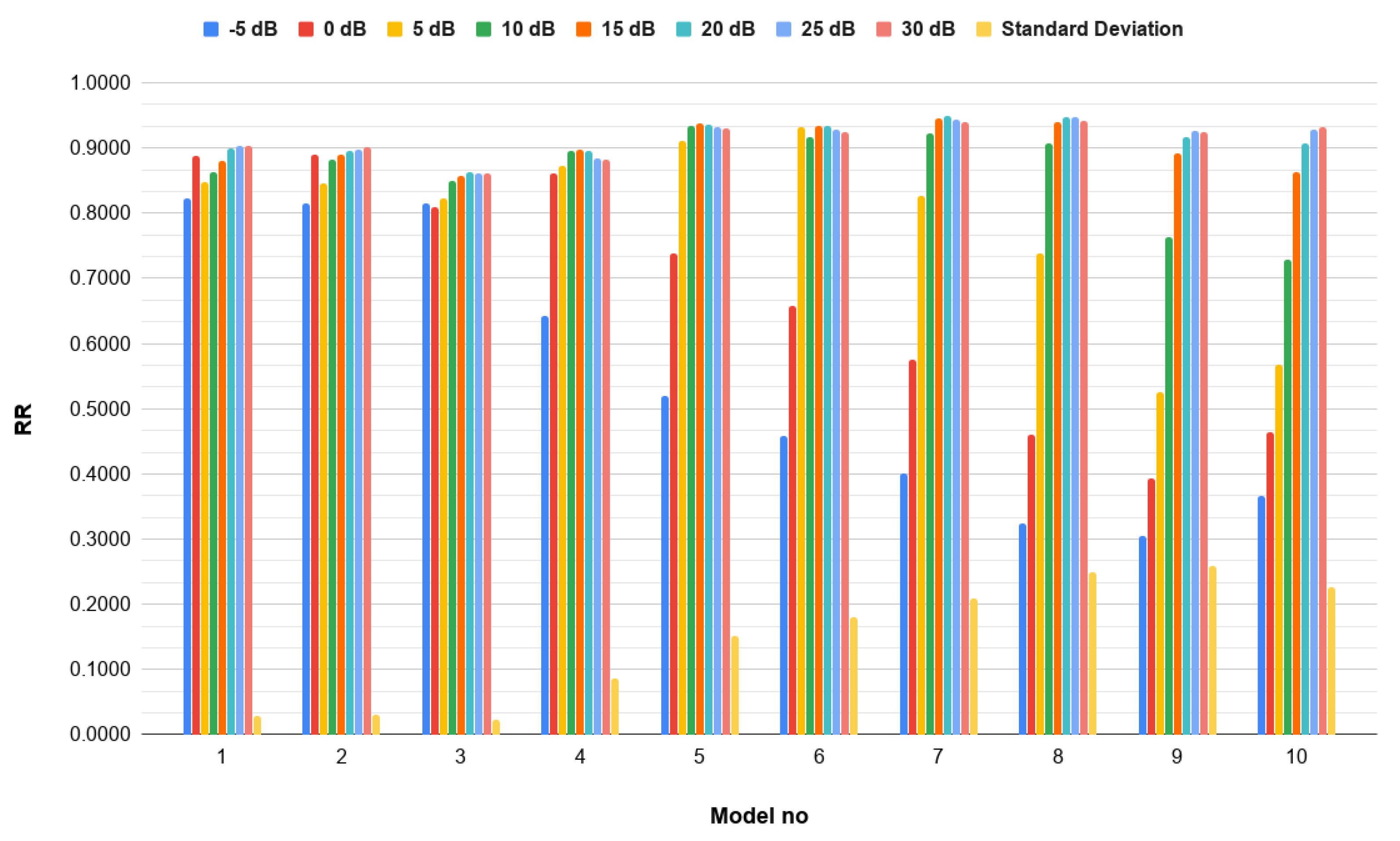
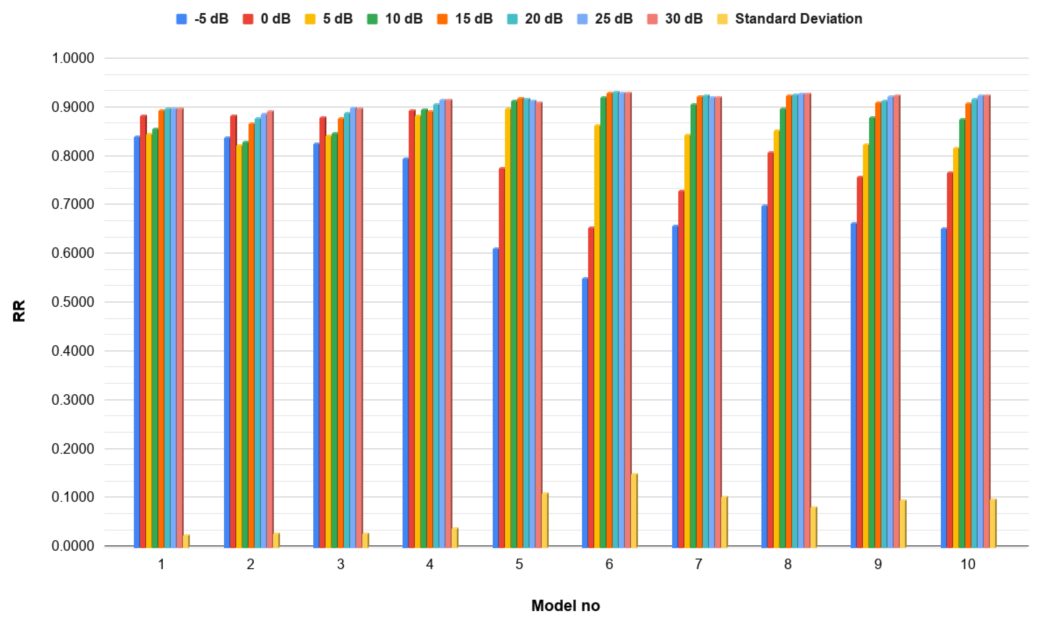
Within an event-based evaluation framework, an event is considered correctly detected if at least one of the time windows which overlap it is properly classified. Four metrics are adopted in this study: Recognition Rate (RR), Miss Detection Rate (MDR), Error Rate (ER) and False Positive Rate (FPR). For the single-channel experiments, precision, recall and F1-Score were selected as the evaluation metrics. The error count can be obtained by subtracting the detection and miss counts from the number of events presented to the model. The values are normalized by the number of events. It must be noted at this point that, to the best of the authors’ knowledge, the detection protocol performed on the MIVIA Audio Events Dataset is typically event-based, meaning that an event of interest (namely GB, G and S), is considered correctly detected if it is identified for at least one of the consecutive sequence of frames in which it appears. The frame-by-frame results are also reported, in which RR, MDR, ER and FPR are computed by considering the total number of audio frames (total number of magnitude representations).

3.3. Results

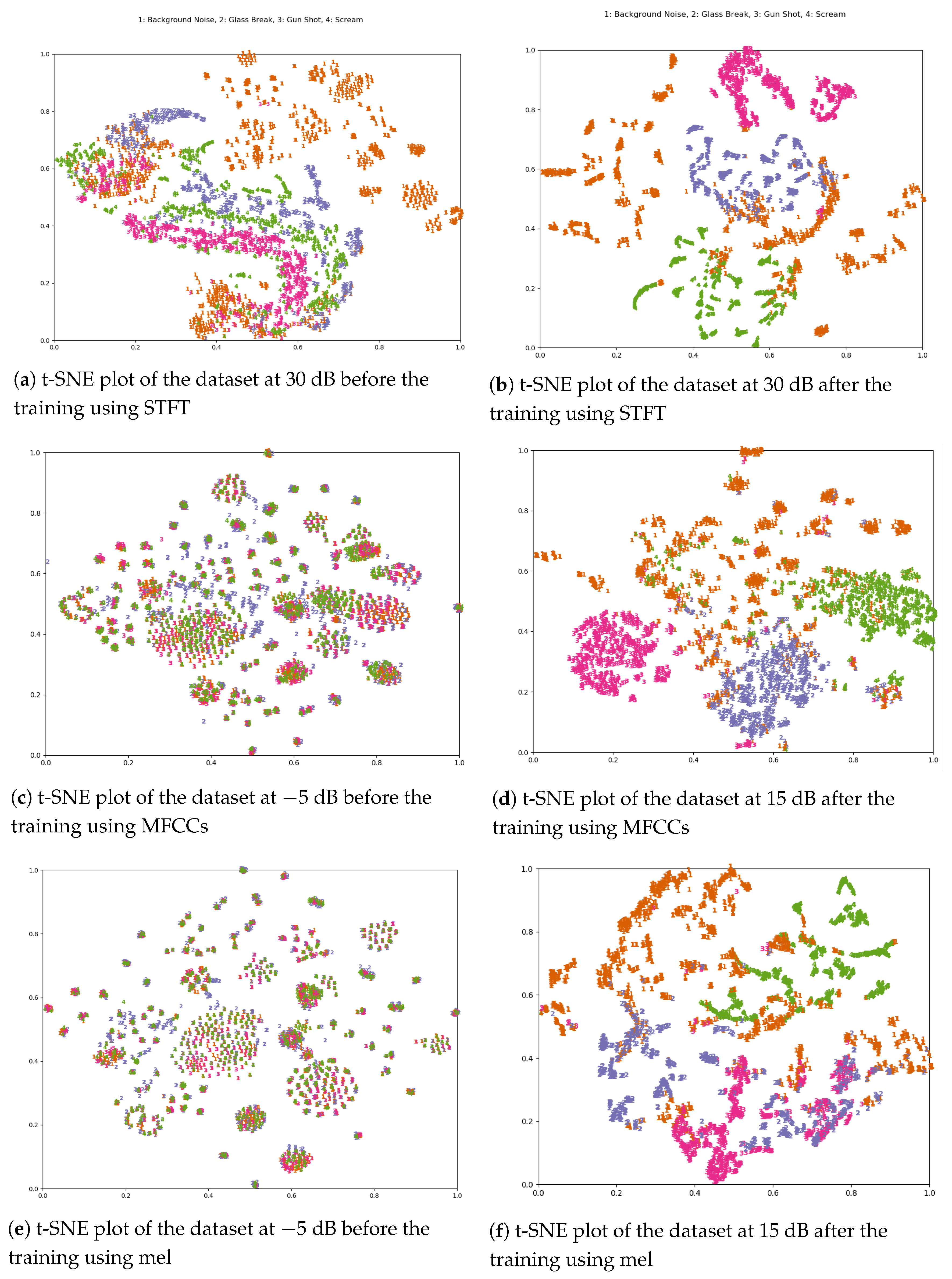
3.3.1. Single-Channel Spectrograms

The single-channel spectrogram results are summarized in Table 2. The main focus of the experiment is to evaluate the ability of a 2D CNN to learn from various spectrogram representations at various SNR settings and to check the ability of the CNN to generalize on different SNR settings during training and testing. The STFT spectrograms provided the best results when training and testing on the same SNR values, compared to mel-spectrograms which are focused on the mel-scale to better represent the human auditory system. This result means that, for environmental sounds, there should not be any amplitude boost given at certain frequencies. Instead, all frequencies in the spectrum should be treated equally. Figure 2 depicts the T-distributed Stochastic Neighbor Embedding (t-SNE) plot (BN: orange color, GB: purple color, G: pink color and S: green color) of the dataset before training, on the left, and the features learnt by DenseNet-121 after training. The top plot shows the ability of DenseNet-121 to learn and form class clusters when trained and tested using the STFT spectrograms at 30 dB. The middle plot shows the ability of the generalization, using the MFCC spectrograms, at $-5$ dB for training and 15 dB for testing, and the bottom plot depicts the poor generalization results of the mel-spectrograms at $-5$ dB for training and 15 dB for testing. T-distributed Stochastic Neighbor Embedding (t-SNE) is a nonlinear dimensionality reduction technique well-suited for embedding high-dimensional data for visualization in a low-dimensional space of two or three dimensions. It serves the purpose of visualization of the features learned during training, and its process is twofold; it constructs a probability distribution over pairs of high-dimensional objects in a way that similar objects are assigned a higher probability while dissimilar points are assigned a lower probability. After that, t-SNE defines a similar probability distribution over the points in the low-dimensional map and it minimizes the Kullback–Leibler divergence (KL divergence, [48]) between the two distributions with respect to the locations of the points in the map.

In general, the network is able to accurately cluster the Glass Break, Gunshot and Scream classes, whereas the Background Noise that contains a variety of environmental audio signals forms a wider cluster over the t-SNE space. On the contrary, it is noticeable that the model trained on the MFCCs is able to generalize better than the STFT spectrogram and the mel-spectrogram when they are trained and tested on different SNR settings. This can be explained since the MFCC magnitude representation includes all the important information of the audio signal in the lowest MFCC features (e.g., first 10 features) in terms of concentrated energies and has minimum changes in the highest ones. Therefore, the network is able to learn all the patterns in the lowest part of the magnitude representation.

3.3.2. Multichannel Spectrograms

A representative sample of the variation with respect to each class and SNR in the extended dataset is shown in Figure 3. It is evident that, as the SNR increases, the features become clearer and easier to distinguish from the background, as was expected.

Although the focus of the present study is mainly on multichannel spectrogram representation performance (as well as studying different single channel representations) and the study of the effect of the SNR on the performance, a comparison of different studies conducted on the MIVIA Audio Events dataset is shown in

Table 3. Results (frame-by-frame) of available studies in the literature along with the results of the current work, regarding the four classes (including the background noise) of the original and the extended MIVIA Audio Events Dataset: apart from the four metrics presented in Section 3.2, the accuracy is also shown, for comparison reasons only.

Method Test with SNR > 0	Representation	RR (%)	Accuracy (%)	MDR (%)	ER (%)	FPR (%)
Present Study	STFT + Mel + MFCC (Stacked)	92.5	95.21	7.28	0.22	2.59
COPE [19]	Gammatonegram	96	-	3.1	0.9	4.3
AReN [30] ${}^1$	Gammatonegram	94.65	-	4.97	0.38	0.78
SoundNet [19]	Gammatonegram	93.33	-	9.9	1.4	1.4
bof${}_s$ [11]	Gammatonegram	86.7	-	9.65	1.4	3.1
bof${}_h$ [11]	Gammatonegram	84.8	-	12.5	2.7	2.1
SoreNet [29] ${}^1$	Spectrogram	-	88.9	-	-	-
AENet [29] ${}^1$	Spectrogram	-	81.5	-	-	-
AENet [30] ${}^1$	Gammatonegram	88.73	-	8.84	2.43	2.59
AENet [30] ${}^1$	Spectrogram	78.82	-	16.69	4.48	5.35
Test with SNR > 0 and SNR ≤ 0
Present Study	STFT + Mel + MFCC (Stacked)	90.45	93.88	8.47	0.62	3.68
COPE [19]	Gammatonegram	91.7	-	2.61	5.68	9.2
SoundNet [19]	Gammatonegram	84.13	-	4	11.88	25.9
bof${}_s$ [11]	Gammatonegram	59.11	-	32.97	7.92	5.3
bof${}_h$ [11]	Gammatonegram	56.07	-	36.43	7.5	5.3

${}^1$ The authors report training on 50,000 and testing on 33,000 magnitude representations, while in the rest of the studies (including the current) the corresponding numbers were 70,770 and 30,348 for the original and 94,360 and 40,464 for the extended dataset, respectively.

. The two common representations mentioned in the literature are spectrograms and gammatonegrams. The former is the traditional time-frequency visualization, but it actually has some important differences from how sound is analyzed by the ear; most significantly, the ear’s frequency sub-bands get wider for higher frequencies, whereas the spectrogram has a constant bandwidth across all frequency channels. A Gammatone spectrogram or gammatonegram is a time-frequency magnitude array based on an FFT-based approximation to gammatone sub-band filters, for which the bandwidth increase with increasing central frequency. The upper part of the table compares the results achieved by considering the classification of positive SNR sound events only are shown. In the lower part of the Table, the results achieved by including sound events with negative and null SNR to the above are exhibited. Furthermore, in

Table 4. Classification matrices obtained from the multichannel approach for the original and extended MIVIA audio events data set: GB, GS and S indicate the classes in the dataset (Table 1), while MDR is the miss-detection rate. The class BN is excluded for a one-to-one comparison with [19].

	Original dataset
	GB	G	S	MDR
GB	91.48%	0.35%	0%	8.17%
G	0.11%	98.46%	0.02%	1.41%
S	0.02%	0.31%	87.41%	12.26%
	Extended dataset
	GB	G	S	MDR
GB	94.68%	0.44%	0.15%	4.72%
G	0.1%	95.4%	0.43%	4.07%
S	0.24%	0.5%	82.64%	16.63%

, classification matrices obtained on both original and extended datasets using the multichannel (stacked) approach are shown. The average RRs for the three classes of interest (event-based) were 92.5% and 90.9% for the original and the extended dataset, respectively. The latter compares well with the reported value of 90.7% in [19].

As was discussed in Section 3.2, ten models were trained in total for both single-channel concatenated and multichannel stacked representations of the raw audio. The performance of each model for the former and latter methods is shown in Figure 4 and Figure 5, respectively. In both cases, it was evident that the zero or negative SNR values were the most challenging, as can be seen in Figure 3. For that reason, the three models trained on $-5$ dB (models 1, 2 and 3) performed better than the rest in terms of generalization and consistency throughout all SNR values. Indicatively, the standard deviation for the RR scores attained with these models was about 0.03 in both the concatenated and stacked input methods. This value increased as the SNR value of the training set increased, reaching approximately 0.33 and 0.25 using the former and latter method, respectively. The above combined with the results in Figure 4 and Figure 5 suggest that the stacked input method exhibited a higher generalization capacity than that of the concatenated features method.

In Figure 6, the generalization capabilities of the two multichannel methods are shown in terms of event-based recognition (GB, G and S). As one moves along the sequence of the ten models (

Table 5. A list of multichannel models in terms of the SNRs chosen for training and testing.

Model No	Training SNR (dB)	Testing SNR (dB)
1	$-5$	$-15$
2	$-5$	30
3	$-5$	$-5$
4	0	0
5	5	5
6	10	10
7	15	15
8	20	20
9	25	25
10	30	30

), it is evident that the generalization capabilities of the stacked multichannel method are significantly better than the corresponding concatenated multichannel method. In both cases, the model that was trained in $-5$ dB and tested in 15 dB showed the best performance, with a recognition score of 91.51% for the concatenated method and 90.23% for the stacked method, with the lowest standard deviation, namely 0.034 and 0.019, respectively. Moving up in terms of SNR training (and model number), it became more difficult to generalize, especially in the case of zero and below SNRs. This is due to the fact that the lower SNR audio contains higher levels of noise (Figure 3) and thus is more challenging, leading to more robust and generalizable classification.

3.4. Experimental Analysis and Discussion

As was seen in Section 3, when comparing single-channel representations, the MFCC is able to generalize better than the STFT spectrogram and the mel-spectrogram. This most probably owes to the fact that this representation includes all the important information of the audio signal in the lowest MFCC features (e.g., first 10 features) with regard to concentrated energies and has minimum changes in the highest ones. Hence, it is suggested that it has its place in a feature representation combination, and for that reason, it was indeed used in both methods of multichannel representation (Section 2.3).

With regard to the multichannel representation, the stacked features method proved to be more generalizable compared to the concatenated features method, especially when training was carried out on higher SNRs and testing was carried out on lower ones. Neither the concatenated features method nor separate single-channel spectrogram representations (STFT, mel or MFCC) performed as well.

Generalization on Unseen Data

One of the most challenging public audio datasets is the UrbanSound8K dataset [49]. It contains 8732 labeled sound excerpts (≤4 s) of urban sounds from 10 classes: air conditioner, car horn, children playing, dog bark, drilling, engine idling, gunshot, jackhammer, siren and street music. It consists of ten predefined folds (splits). There is a couple of common oversights when analyzing this dataset: data reshuffling and testing on only one of the splits. If the data is reshuffled (i.e., combined from all folds with a random train/test split generated), related samples will be incorrectly placed in both the train and test sets. That would lead to inflated scores due to data leakage that do not represent the model’s performance on unseen data. Testing on only one of the ten folds is considered insufficient, as each fold is of varying classification difficulty. According to the dataset provider, models tend to obtain much higher scores when trained on folds 1–9 and tested on fold 10 compared to training on, e.g., folds 2–10 and testing on fold 1. Consequently, following the predefined folds protocol in [49] ensures comparability with existing results in the literature.

The aforementioned dataset was selected for generalization testing of the models in the present study due to the fact that it contains one common class with the MIVIA Audio Events dataset, namely the gunshot (G) class. Owing to the fact that it is an imbalanced dataset, the number of excerpts in which this class is present is 374 (out of a total of 8732, which is approximately 4% of the dataset).

The procedure that was used for input generation was the stacked multichannel magnitude representation. Following the predefined folds protocol, each predefined fold was used for testing of each of the ten models that was trained on the MIVIA Audio Events dataset (Table 5). The results are presented in Figure 7.

When using the models trained on or below 10 dB SNRs on the MIVIA Audio Events dataset, the recognition rate ranged between 49% and 75% (still comparing well with models in the literature originally trained on the UrbanSound8K dataset, e.g., 0% [50]). This is not the case when using the rest of the models (trained on or above 15 dB SNRs), as it can be seen that the results from the present study compare well with the state-of-the-art recognition rate (Salomon and Bello [26], 94%), varying from 91% to 97% for the class of interest. Given that the models were not trained on the UrbanSound8K dataset and that the dataset mainly consists of higher SNR audio events, the above results would suggest the generalization capability of the stacked multichannel representation approach.

4. Conclusions

Microphone distance, ambient noise and SNR are well-known challenges in audio analysis and classification; they are factors that differentiate the latter from fields that have proven more straightforward for image analysis. The present work’s aim was to tackle the aforementioned issues and to provide a form of analysis that generalizes well even when background noise is high and/or the signal of the event of interest is weak and the SNR drops to the negative territory. One major field that would benefit from anomaly detection via audio event recognition without using speech recognition is surveillance in AVs. To the best of the authors’ knowledge, a comparative analysis of the performance and the generalization capabilities of a series of models and combinations of input features (spectrogram types, single- and multichannel combinations, etc.) is reported for the first time in the present study.

In terms of single channels, MFCC magnitude proved the most generalizable representation of the three studied in the present work; hence, it was used as one of the three components in both multichannel methods. The combination of the aforementioned three magnitude spectrogram representations in a summed up representation was able to generalize when trained only on low SNRs. The event-based recognition rate was comparable to other systems in the literature that were trained on all SNR values of the MIVIA dataset. Furthermore, the proposed method generalizes well in terms of recognizing a common class (gunshot) in an unseen during training dataset (UrbanSound8K) when using the models trained in sounds with an SNR greater than 15 dB.

This generalizability, benefiting from the method of combining audio features can open a new pathway of leveraging on audio to successfully monitor the inside and outside environments of an AV and to significantly improve anomaly detection.

References

1. Räty, T.D. Survey on contemporary remote surveillance systems for public safety. IEEE Trans. Syst. Man Cybern. Part C Appl. Rev. 2010, 40, 493–515. [Google Scholar] [CrossRef]
2. Bramberger, M.; Doblander, A.; Maier, A.; Rinner, B.; Schwabach, H. Distributed embedded smart cameras for surveillance applications. Computer 2006, 39, 68–75. [Google Scholar] [CrossRef]
3. Elmaghraby, A.S.; Losavio, M.M. Cyber security challenges in Smart Cities: Safety, security and privacy. J. Adv. Res. 2014, 5, 491–497. [Google Scholar] [CrossRef] [PubMed] [Green Version]
4. Research, B. Global OR Visualization Systems Market Focus on Systems (OR Camera Systems, OR Display Systems, OR Video Systems, and Surgical Light Sources), Regions (16 Countries), and Competitive Landscape—Analysis and Forecast, 2019–2025. 2019. Available online: businesswire.com/news/home/20190618005416/en/Global-Visualization-Systems-Market-2019-2025-Focus-Camera (accessed on 24 July 2020).
5. Salamanis, A.; Kehagias, D.D.; Filelis-Papadopoulos, C.K.; Tzovaras, D.; Gravvanis, G.A. Managing spatial graph dependencies in large volumes of traffic data for travel-time prediction. IEEE Trans. Intell. Transp. Syst. 2015, 17, 1678–1687. [Google Scholar] [CrossRef]
6. Bösch, P.M.; Becker, F.; Becker, H.; Axhausen, K.W. Cost-based analysis of autonomous mobility services. Transp. Policy 2018, 64, 76–91. [Google Scholar] [CrossRef]
7. Brun, L.; Saggese, A.; Vento, M. Dynamic scene understanding for behavior analysis based on string kernels. IEEE Trans. Circuits Syst. Video Technol. 2014, 24, 1669–1681. [Google Scholar] [CrossRef]
8. Valera, M.; Velastin, S.A. Intelligent distributed surveillance systems: A review. IEE Proc.-Vis. Image Signal Process. 2005, 152, 192–204. [Google Scholar] [CrossRef]
9. Crocco, M.; Cristani, M.; Trucco, A.; Murino, V. Audio surveillance: A systematic review. ACM Comput. Surv. CSUR 2016, 48, 1–46. [Google Scholar] [CrossRef]
10. Foggia, P.; Saggese, A.; Strisciuglio, N.; Vento, M.; Petkov, N. Car crashes detection by audio analysis in crowded roads. In Proceedings of the 2015 12th IEEE International Conference on Advanced Video and Signal Based Surveillance (AVSS), Karlsruhe, Germany, 25–28 August 2015; pp. 1–6. [Google Scholar]
11. Foggia, P.; Petkov, N.; Saggese, A.; Strisciuglio, N.; Vento, M. Audio surveillance of roads: A system for detecting anomalous sounds. IEEE Trans. Intell. Transp. Syst. 2015, 17, 279–288. [Google Scholar] [CrossRef]
12. Lopatka, K.; Kotus, J.; Czyzewski, A. Detection, classification and localization of acoustic events in the presence of background noise for acoustic surveillance of hazardous situations. Multimed. Tools Appl. 2016, 75, 10407–10439. [Google Scholar] [CrossRef] [Green Version]
13. Conte, D.; Foggia, P.; Percannella, G.; Saggese, A.; Vento, M. An ensemble of rejecting classifiers for anomaly detection of audio events. In Proceedings of the 2012 IEEE Ninth International Conference on Advanced Video and Signal-Based Surveillance, Beijing, China, 18–21 September 2012; pp. 76–81. [Google Scholar]
14. Saggese, A.; Strisciuglio, N.; Vento, M.; Petkov, N. Time-frequency analysis for audio event detection in real scenarios. In Proceedings of the 2016 13th IEEE International Conference on Advanced Video and Signal Based Surveillance (AVSS), Colorado Springs, CO, USA, 23–26 August 2016; pp. 438–443. [Google Scholar]
15. Besacier, L.; Barnard, E.; Karpov, A.; Schultz, T. Automatic speech recognition for under-resourced languages: A survey. Speech Commun. 2014, 56, 85–100. [Google Scholar] [CrossRef]
16. Fu, Z.; Lu, G.; Ting, K.M.; Zhang, D. A survey of audio-based music classification and annotation. IEEE Trans. Multimed. 2010, 13, 303–319. [Google Scholar] [CrossRef]
17. Roy, A.; Doss, M.M.; Marcel, S. A fast parts-based approach to speaker verification using boosted slice classifiers. IEEE Trans. Inf. Forensics Secur. 2011, 7, 241–254. [Google Scholar] [CrossRef]
18. Vafeiadis, A.; Votis, K.; Giakoumis, D.; Tzovaras, D.; Chen, L.; Hamzaoui, R. Audio content analysis for unobtrusive event detection in smart homes. Eng. Appl. Artif. Intell. 2020, 89, 103226. [Google Scholar] [CrossRef] [Green Version]
19. Strisciuglio, N.; Vento, M.; Petkov, N. Learning representations of sound using trainable COPE feature extractors. Pattern Recognit. 2019, 92, 25–36. [Google Scholar] [CrossRef] [Green Version]
20. Asadi-Aghbolaghi, M.; Clapes, A.; Bellantonio, M.; Escalante, H.J.; Ponce-López, V.; Baró, X.; Guyon, I.; Kasaei, S.; Escalera, S. A survey on deep learning based approaches for action and gesture recognition in image sequences. In Proceedings of the 2017 12th IEEE International Conference on Automatic Face & Gesture Recognition (FG 2017), Washington, DC, USA, 30 May–3 June 2017; pp. 476–483. [Google Scholar]
21. Gao, M.; Jiang, J.; Zou, G.; John, V.; Liu, Z. RGB-D-based object recognition using multimodal convolutional neural networks: A survey. IEEE Access 2019, 7, 43110–43136. [Google Scholar] [CrossRef]
22. Sindagi, V.A.; Patel, V.M. A survey of recent advances in cnn-based single image crowd counting and density estimation. Pattern Recognit. Lett. 2018, 107, 3–16. [Google Scholar] [CrossRef] [Green Version]
23. Xia, R.; Liu, Y. A multi-task learning framework for emotion recognition using 2D continuous space. IEEE Trans. Affect. Comput. 2015, 8, 3–14. [Google Scholar] [CrossRef]
24. Guo, F.; Yang, D.; Chen, X. Using deep belief network to capture temporal information for audio event classification. In Proceedings of the 2015 International Conference on Intelligent Information Hiding and Multimedia Signal Processing (IIH-MSP), Adelaide, Australia, 23–25 September 2015; pp. 421–424. [Google Scholar]
25. Wang, C.Y.; Wang, J.C.; Santoso, A.; Chiang, C.C.; Wu, C.H. Sound event recognition using auditory-receptive-field binary pattern and hierarchical-diving deep belief network. IEEE ACM Trans. Audio Speech Lang. Process. 2017, 26, 1336–1351. [Google Scholar] [CrossRef]
26. Salamon, J.; Bello, J.P. Deep convolutional neural networks and data augmentation for environmental sound classification. IEEE Signal Process. Lett. 2017, 24, 279–283. [Google Scholar] [CrossRef]
27. Zhang, H.; McLoughlin, I.; Song, Y. Robust sound event recognition using convolutional neural networks. In Proceedings of the 2015 IEEE International Conference on Acoustics, Speech and Signal Processing (ICASSP), Brisbane, Australia, 19–24 April 2015; pp. 559–563. [Google Scholar]
28. Takahashi, N.; Gygli, M.; Van Gool, L. Aenet: Learning deep audio features for video analysis. IEEE Trans. Multimed. 2017, 20, 513–524. [Google Scholar] [CrossRef] [Green Version]
29. Greco, A.; Saggese, A.; Vento, M.; Vigilante, V. SoReNet: A novel deep network for audio surveillance applications. In Proceedings of the 2019 IEEE International Conference on Systems, Man and Cybernetics (SMC), Bari, Italy, 6–9 October 2019; pp. 546–551. [Google Scholar]
30. Greco, A.; Petkov, N.; Saggese, A.; Vento, M. AReN: A Deep Learning Approach for Sound Event Recognition using a Brain inspired Representation. IEEE Trans. Inf. Forensics Secur. 2020, 15, 3610–3624. [Google Scholar] [CrossRef]
31. Hertel, L.; Phan, H.; Mertins, A. Comparing time and frequency domain for audio event recognition using deep learning. In Proceedings of the 2016 International Joint Conference on Neural Networks (IJCNN), Vancouver, BC, Canada, 24–29 July 2016; pp. 3407–3411. [Google Scholar]
32. Mesaros, A.; Heittola, T.; Benetos, E.; Foster, P.; Lagrange, M.; Virtanen, T.; Plumbley, M.D. Detection and classification of acoustic scenes and events: Outcome of the DCASE 2016 challenge. IEEE ACM Trans. Audio Speech Lang. Process. 2017, 26, 379–393. [Google Scholar] [CrossRef] [Green Version]
33. Abadi, M.; Agarwal, A.; Barham, P.; Brevdo, E.; Chen, Z.; Citro, C.; Corrado, G.S.; Davis, A.; Dean, J.; Devin, M.; et al. TensorFlow: Large-Scale Machine Learning on Heterogeneous Systems. arXiv 2015, arXiv:1603.04467. [Google Scholar]
34. Oliphant, T.E. A Guide to Numpy; Trelgol Publishing USA: New York, NY, USA, 2006; Volume 1. [Google Scholar]
35. McKinney, W. Data Structures for Statistical Computing in Python. In Proceedings of the 9th Python in Science Conference, Austin, TX, USA, 28 June–3 July 2010. [Google Scholar] [CrossRef] [Green Version]
36. Hunter, J.D. Matplotlib: A 2D graphics environment. Comput. Sci. Eng. 2007, 9, 90–95. [Google Scholar] [CrossRef]
37. Virtanen, P.; Gommers, R.; Oliphant, T.E.; Haberland, M.; Reddy, T.; Cournapeau, D.; Burovski, E.; Peterson, P.; Weckesser, W.; Bright, J.; et al. SciPy 1.0: Fundamental algorithms for scientific computing in Python. Nat. Methods 2020, 17, 261–272. [Google Scholar] [CrossRef] [Green Version]
38. McFee, B.; Raffel, C.; Liang, D.; Ellis, D.P.; McVicar, M.; Battenberg, E.; Nieto, O. Librosa: Audio and music signal analysis in python. In Proceedings of the 14th Python in Science Conference, Austin, TX, USA, 6–12 July 2015; Volume 8, pp. 18–25. [Google Scholar]
39. Sanner, M.F. Python: A programming language for software integration and development. J. Mol. Graph. Model. 1999, 17, 57–61. [Google Scholar]
40. Bradski, G.; Kaehler, A. Learning OpenCV: Computer Vision with the OpenCV Library; O’Reilly Media, Inc.: Sebastopol, CA, USA, 2008. [Google Scholar]
41. Kumar, T.; Verma, K. A Theory Based on Conversion of RGB image to Gray image. Int. J. Comput. Appl. 2010, 8, 7–10. [Google Scholar]
42. Zinemanas, P.; Cancela, P.; Rocamora, M. End-to-end convolutional neural networks for sound event detection in urban environments. In Proceedings of the 2019 24th Conference of Open Innovations Association (FRUCT), Moscow, Russia, 8–12 April 2019; pp. 533–539. [Google Scholar]
43. Huang, G.; Liu, Z.; Van Der Maaten, L.; Weinberger, K.Q. Densely connected convolutional networks. In Proceedings of the IEEE Conference on Computer Vision and Pattern Recognition, Honolulu, HI, USA, 21–26 July 2017; pp. 4700–4708. [Google Scholar]
44. Sandler, M.; Howard, A.; Zhu, M.; Zhmoginov, A.; Chen, L.C. Mobilenetv2: Inverted residuals and linear bottlenecks. In Proceedings of the IEEE Conference on Computer Vision and Pattern Recognition, Salt Lake City, UT, USA, 18–22 June 2018; pp. 4510–4520. [Google Scholar]
45. He, K.; Zhang, X.; Ren, S.; Sun, J. Deep residual learning for image recognition. In Proceedings of the IEEE Conference on Computer Vision and Pattern Recognition, Las Vegas, NV, USA, 27–30 June 2016; pp. 770–778. [Google Scholar]
46. Foggia, P.; Petkov, N.; Saggese, A.; Strisciuglio, N.; Vento, M. Reliable detection of audio events in highly noisy environments. Pattern Recognit. Lett. 2015, 65, 22–28. [Google Scholar] [CrossRef]
47. Kingma, D.P.; Ba, J. Adam: A method for stochastic optimization. In Proceedings of the 3rd International Conference for Learning Representations (ICLR-15), Banff, AB, Canada, 14–16 April 2014. [Google Scholar]
48. Kullback, S.; Leibler, R.A. On Information and Sufficiency. Ann. Math. Statist. 1951, 22, 79–86. [Google Scholar] [CrossRef]
49. Salamon, J.; Jacoby, C.; Bello, J.P. A dataset and taxonomy for urban sound research. In Proceedings of the 22nd ACM International Conference on Multimedia, Orlando, FL, USA, 3–7 November 2014; pp. 1041–1044. [Google Scholar]
50. Davis, N.; Suresh, K. Environmental sound classification using deep convolutional neural networks and data augmentation. In Proceedings of the 2018 IEEE Recent Advances in Intelligent Computational Systems (RAICS), Thiruvananthapuram, India, 6–8 December 2018; pp. 41–45. [Google Scholar]
Figure 1. The two representation methods, described in Section 2.3: the concatenation method is shown on top, and the stacking method is on the bottom.
Electronics 09 01593 g001
Figure 2. T-distributed Stochastic Neighbor Embedding (t-SNE) plots of the Short-Time Fourier Transform (STFT) (top), Mel-Frequency Cepstral Coefficients (MFCCs) (middle) and mel (bottom). BN: orange color, GB: purple color, G: pink color and S: green color. The x-axis shows t-SNE dimension 1, and the y-axis shows t-SNE dimension 2.
Electronics 09 01593 g002
Figure 3. Multichannel spectrograms obtained with the stacked method discussed in Section 2: the representations of the four classes of the extended dataset are shown, with the SNR value increasing at the direction of the arrow (left side) from 5 dB to 30 dB with a step of 5 dB.
Electronics 09 01593 g003
Figure 4. Frame-by-frame Recognition Rate (RR) for all models using concatenated features from STFT, mel and MFCC spectrograms (single channel) validated for each Signal-to-Noise Ratio (SNR): each column group refers to a specific model (see Table 5).
Electronics 09 01593 g004
Figure 5. Frame-by-frame RR for all models using stacked features from STFT, mel and MFCC spectrograms (multichannel) validated for each SNR: each column group refers to a specific model (see Table 5).
Electronics 09 01593 g005
Figure 6. A comparison of the models trained with the concatenated (top) and stacked (bottom) features method with regard to event-based RR: the sequence of the models increases from 1 to 10, as per Table 5.
Electronics 09 01593 g006
Figure 7. Statistics for each of the models obtained in the present study for the Gunshot (G) event class of the UrbanSound8K dataset.
Electronics 09 01593 g007