Abstract
Recent speech enhancement research has shown that deep learning techniques are very effective in removing background noise. Many deep neural networks are being proposed, showing promising results for improving overall speech perception. The Deep Multilayer Perceptron, Convolutional Neural Networks, and the Denoising Autoencoder are well-established architectures for speech enhancement; however, choosing between different deep learning models has been mainly empirical. Consequently, a comparative analysis is needed between these three architecture types in order to show the factors affecting their performance. In this paper, this analysis is presented by comparing seven deep learning models that belong to these three categories. The comparison includes evaluating the performance in terms of the overall quality of the output speech using five objective evaluation metrics and a subjective evaluation with 23 listeners; the ability to deal with challenging noise conditions; generalization ability; complexity; and, processing time. Further analysis is then provided while using two different approaches. The first approach investigates how the performance is affected by changing network hyperparameters and the structure of the data, including the Lombard effect. While the second approach interprets the results by visualizing the spectrogram of the output layer of all the investigated models, and the spectrograms of the hidden layers of the convolutional neural network architecture. Finally, a general evaluation is performed for supervised deep learning-based speech enhancement while using SWOC analysis, to discuss the technique’s Strengths, Weaknesses, Opportunities, and Challenges. The results of this paper contribute to the understanding of how different deep neural networks perform the speech enhancement task, highlight the strengths and weaknesses of each architecture, and provide recommendations for achieving better performance. This work facilitates the development of better deep neural networks for speech enhancement in the future.
1. Introduction
Speech enhancement is the process of improving the quality and intelligibility of a speech signal by removing any other signals propagating with it, being defined as noise. There are many applications for speech enhancement, for example, it is an essential process in hearing aids, mobile communication systems, Automatic Speech Recognition (ASR), headphones, and VoIP (Voice over IP) communication [1]. Speech enhancement is a longstanding issue that has attracted the attention of signal processing researchers for decades and it remains unsolved. Many techniques have been proposed in order to tackle this challenging task, starting from the classical techniques that were first proposed in the 70s [2], which are based on statistical assumptions of the noise presented in the speech signal, to the more advanced techniques that researchers have reached nowadays, based on deep learning algorithms [3]. The classical techniques have been previously widely used, and they are based on analyzing the relationship between speech and noise while using statistical assumptions. Although some of these techniques were reported to be effective in enhancing the noisy speech [4,5], it was proven that these methods are more effective when applied to environments with a relatively high Signal to Noise Ratio (SNR), or in the case of stationary noise conditions [2]. It was also reported that these techniques are not effective in improving speech intelligibility [6,7]. However, in deep learning-based supervised speech enhancement, a Deep Neural Network (DNN) is trained while using pairs of clean and noisy speech signals, in order to learn the mapping function that gives the best prediction of the clean speech without using any statistical assumptions [8].
Deep learning-based speech enhancement has made a clear contribution in this research area, and some proposed DNNs have managed to output speech with much better perception, as compared to the classical techniques. However, the learning process of a DNN for speech enhancement is affected by many factors, which are summarised in Figure 1. These factors can be divided into three categories: the used model setup, data structure, and learning hyperparameters. In the following Section 1.1, Section 1.2, Section 1.3, these factors are explained in more detail, while the problem definition and contribution of this research will be discussed in Section 1.4.
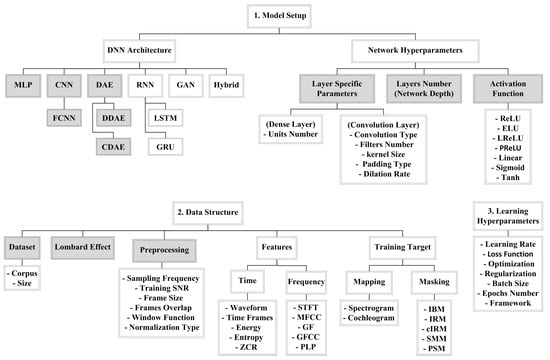
Figure 1.
The three main factors affecting the performance of Deep Neural Networks (DNNs) for speech enhancement: Model Setup, Data Structure, and Learning Hyperparameters. The parts investigated in this study are shaded in grey. All acronyms are defined in Section 1.1, Section 1.2, Section 1.3.
1.1. Model Setup
Many DNN architectures that can perform speech enhancement, including the deep Multilayer Perceptron (MLP), Convolutional Neural Network (CNN), Denoising Autoencoder (DAE), Recurrent Neural Network (RNN), Generative Adversarial Network (GAN), and hybrid architectures. These architectures are discussed in more detail in Section 2. These architectures have their own mathematically defined internal operations [9]; however, the presence of the large numbers of network hyperparameters makes it difficult to determine how much the DNN architecture type is contributing to solving the speech enhancement problem. These hyperparameters include layer-specific parameters, such as the unit number in the case of dense layers; and, the convolution type, number of filters, kernel size, padding type, and dilation rate, in the case of convolution layers [10]. Moreover, the number of layers, or network depth, and the activation functions used are factors that also affect performance [11]. The Rectified Linear Unit (ReLU) [12] and its edited versions: Leaky ReLU (LReLU) [13], Exponential Linear Unit (ELU) [14], and Parametric ReLU (PReLU) [15], are the most commonly used activation functions in the hidden layers. While, Linear, TanH, and Sigmoid are common activation functions in the output layer.
1.2. Data Structure
Deep learning, as a data-driven approach, is also affected by the structure of the data that are used in the training process. The speech and noise corpora and their sizes highly impact the learning process. Moreover, it is common to do some preprocessing operations before feeding the data to a DNN for speech enhancement, such as choosing between 8 kHz and 16 kHz sampling frequency in order to feed the network with the most relevant band of speech frequencies; the frame size used, frame overlap percentage, and the window function [16] in order to ensure the efficiency of the training process; the used normalization type to ensure generalization and facilitate the training process [17]; and, the chosen training SNR to adjust the intensity of the background noise. The chosen setup for all of these preprocessing operations affects the performance of the DNN.
Another factor that has a great impact on performance is the representation of the speech signal in either time or frequency, as different speech features that can be extracted based on the chosen representation. In the time domain, it is common to use the original representation of the waveform or use short time frames and extract some features, such as energy, entropy, and the Zero Crossing Rate (ZCR) [18]. While, in the frequency domain, many meaningful features can be extracted, including Short Time Fourier Transform (STFT), Mel-Frequency Cepstral Coefficients (MFCC) [19], Gammatone Frequency (GF), Gammatone Frequency Cepstral Coefficients (GFCC) [20], and Perceptual Linear Prediction (PLP) [21].
The training target is another factor that affects performance. With speech enhancement, the training target is one of two types: mapping or masking [22,23]. The problem can be seen as a regression problem if the target is mapping to clean speech time frames, spectrogram, or cochleagram. It can also be considered to be a classification problem if the target is to produce a mask that classifies every portion of the signal as either speech or noise, and then by weighting the noisy speech with this mask, the enhanced speech signal can be generated. There are many masking targets used in speech enhancement, such as Ideal Binary Mask (IBM) [24], Ideal Ratio Mask (IRM) [25], and Spectral Magnitude Mask (SMM); also known as Fast Fourier Transform mask (FFT-mask) [22], complex Ideal Ratio Mask (cIRM) [26], and Phase-Sensitive Mask (PSM) [27].
1.3. Learning Hyperparamters
The learning process of a DNN also has some hyperparameters, such as the learning rate, loss function, optimization technique, regularization technique, batch size, number of epochs, and the framework that was chosen for implementation [28]. The setup of all these hyperparameters is the third factor that impacts the performance of DNNs for speech enhancement.
1.4. Problem Definition and Research Contribution
Because deep learning is affected by so many factors, understanding how DNNs work through the investigation of these factors is a controversial subject in many research areas, including speech enhancement. The study in [29] investigated the use of different speech features for a classification task in order to estimate the IBM at low SNR. In Reference [30], an investigation is presented on the two speech enhancement learning domains, time, and frequency; while, the work in [31] explains how CNNs learn features from raw audio time series. In Reference [22], the effect of the speech enhancement training targets used for the MLP architecture was studied; and recently, this study was extended to include different architectures [32]. The use of different loss functions for the time domain approach for speech enhancement was also recently evaluated in [33]. Moreover, recommendations were given in [34] for the best values of training hyperparameters: learning rate, batch size, and optimization techniques; while, the work in [35] presents a study of different frameworks that are used in the training process of DNNs.
The outcome of all this research helps in understanding DNNs and aims to change the trial and error nature of the training process. However, further work is needed in order to investigate deep learning-based speech enhancement from the model setup and data structure perspective. Based on the research in the literature, the following gaps were found.
- According to our knowledge, no work was found to compare and analyze the performance of different single channel speech enhancement DNNs, while considering different deep learning and speech enhancement aspects, such as generalization, processing time, challenging noise environments, etc.
- The investigation of network-related hyperparameters, as shown in Figure 1, was not fully covered in the literature.
- The visualization of the hidden layers of CNNs has been effective in understanding how DNNs operate for many research areas; however, this approach was not applied for speech enhancement.
- The effect of data structure related factors, such as preprocessing techniques and the Lombard effect, needs further investigation.
- A general evaluation of deep learning-based speech enhancement is needed in order to highlight its advantages and disadvantages.
In an attempt to fill these research gaps and contribute to the above-mentioned investigations in the literature, the focus of this work is to evaluate different DNNs for single channel supervised speech enhancement and investigate the effect of the chosen model setup and the structure of the data on the performance. This is achieved while using two different investigation approaches: numerical results and spectrogram visualization. The main contributions of this paper are as follows.
- A numerical analysis was conducted on deep learning-based single channel speech enhancement while using the seven best performing DNN speech enhancement architectures. These architectures belong to three broad categories: MLP, CNN, and DAE. The choice of more than one architecture from the same category was based on specific adjustments that were applied to the architecture that makes it perform differently, as discussed in Section 3. The numerical analysis performed covers a complete comparison between the seven architectures, concerning: overall quality of the output speech using objective and subjective metrics, the performance in challenging noise conditions, generalization ability, complexity, and processing time. The outcome of this investigation highlights the advantages and disadvantages of each architecture type.
- Investigating the effect of changing network-related hyperparameters, as shown in Figure 1, to provide recommendations for the best hyperparameter setup.
- Visualizing the spectrograms of the outputs from all the investigated DNNs and the internal layers of a CNN architecture, to give further explanation of the obtained numerical results, obtained from 1 and 2.
- Showing, by numerical analysis, the effect of the data structure on the performance of different DNNs. This investigation includes the effect of the sampling frequency, training SNR, the number of training noise environments, and the Lombard effect. This investigation concludes the best practice setup of training data, and how the Lombard phenomenon will affect testing results.
- A general evaluation was conducted on deep learning-based speech enhancement techniques using SWOC analysis, to reveal its: Strengths, Weaknesses, Opportunities, and Challenges. This evaluation can serve as recommendations for future research.
The rest of this paper is organized, as follows. Section 2 presents a survey of DNN-based speech enhancement architecture types. Section 3 illustrates the details of the implemented seven DNN architectures. Section 4 explains the datasets used and the experimental setups. Section 5 presents the results and discussion of the conducted experiments. The SWOC analysis is discussed in Section 6. Finally, Section 7 provides the conclusion of this paper.
2. DNN Speech Enhancement Architecture Types
Many DNN architecture types have been recently employed for speech enhancement; a review of these types is presented in the following subsections.
2.1. Deep Multi Layer Perceptron (MLP)
An MLP is the most basic and simplest speech enhancement architecture, in which all of the nodes of the network are fully connected. Many speech enhancement DNN models are based on the MLP and they are reported to achieve a significant improvement when compared to the classical approaches. In Reference [36], the authors proposed an MLP network of three hidden layers, while the work shown in [37] is based on four hidden layers, and the use of reverberant speech as a target instead of clean speech, to further improve speech intelligibility in both noisy and reverberant conditions. An MLP architecture is also used in [38], in which 84 speech features feed the network, and unsupervised learning is first used as an initialization process for the network weights, followed by supervised learning for the main training process. The work shown in [39] investigated the large scale training effect on the generalization capability, by training an MLP architecture while using a large number of noise environments. Many other architectures are also found in the literature using MLP for speech enhancement [40,41].
The power of the MLP is its ability to represent the input features and learn the mapping function through the huge number of connections between the layers’ nodes. However, the obvious drawback is the complexity of the architecture due to the huge number of computations, which increases the computational cost and processing time. For that reason, Graphical Processing Units (GPUs) are needed to speed up processing time, but they are more expensive than standard Central Processing Units (CPUs) [42]. Moreover, the fully connected nodes result in a large number of parameters that lead to a big model size that may not fit onto the hardware of some speech enhancement applications [10], such as hearing aids and mobile communication. The MLP also failed to perform time domain-based speech enhancement [30,43] and, because of this, it cannot be considered to be a generalized architecture type.
2.2. Convolutional Neural Network (CNN)
A CNN is an architecture used to solve the computational problem of the MLP by using the convolution operation in both forward and backward propagation steps, in order to reduce network parameters. CNNs were first made for image-related tasks to be able to work with the huge amount of parameters, but, recently, they have proven to be very effective in audio processing [44]. The advantage of the CNN is its dependence on the idea of convolution, which results in fewer network parameters because of parameter sharing and the sparsity of connections. Parameter sharing means that a feature takes advantage of other features in a certain part of the input and uses it in another part, while sparsity of connections means that the output value in each layer does not depend on all of the inputs of the previous layer [45]. Some speech enhancement CNN-based architectures are based on a two-dimensional (2D) convolution, while, recently, 1D convolutions are widely used. One-dimensional (1D) convolution is very effective when applied to sequence data, such as audio processing. Moreover, it results in a lower computational cost, which makes the network suitable for real-time applications [46,47]. The convolution operation also has many hyperparameters, such as padding size, stride size, and dilation rate. Changing these hyperparameters will lead to different types of convolution that impact the performance of the CNN.
CNNs have been widely used in speech enhancement. The work shown in [48] used a CNN-based speech enhancement architecture of 2D convolutions, max pooling, and fully connected layers in order to predict the log power spectra of the clean speech. Another work, [49], is also based on CNN; while, in Reference [43], another version of a CNN is proposed, named Fully CNN (FCNN), in which the fully connected layers are replaced with 2D convolutional layers in an attempt to decrease the computational cost that is added by the fully connected layers. A comparison was also conducted in the same work between the MLP, the basic CNN architecture, and the FCNN for speech enhancement in the time domain, and the results show that the FCNN is the best performing. Recently, the work shown in [50] and [51] used a combination of 1D and 2D dilated convolutions in order to implement a FCNN, and reported a further improvement.
2.3. Denoising Autoencoders (DAE)
The autoencoder is a type of DNN that aims to output a similar representation to the input while using two separate networks: an encoder and decoder. The encoder compresses the input by removing any unimportant information to finally generate a compact form of the input data, and then the decoder reconstructs an estimated form of the input [45]. The autoencoder is considered to be an unsupervised learning scheme, because it only relies on the input data.
Taking advantage of the compression process on the input data in the encoder network, DAEs have been widely used recently in supervised speech enhancement. The idea of DAEs is based on the fact that noise is considered to be unimportant information when trying to map from noisy to clean speech, so it is significantly reduced during the compression process in order to produce clean speech bottleneck features, and then the decoder reconstructs the clean audio [52]. In this case, the autoencoder can be considered as a supervised feature extraction procedure for DNNs, preceding the clean speech prediction task. Bottleneck features have been proven to be very effective and they resulted in significant improvement in many research areas [53,54]
DAEs could be implemented while using any one of the architectures discussed earlier, and they are widely used for speech enhancement. For example, the work done in [55] used an MLP-based autoencoder speech enhancement architecture, also known as Deep DAE (DDAE), while, in Reference [56], a CNN-based one was proposed. A Convolutional DAE (CDAE) is the most commonly used speech enhancement architecture in recent research [50,57,58], because of the lower number of parameters and promising results. However, autoencoders. in general, may not perfectly reconstruct a similar representation of the input, which means the output will experience a loss, and this is the main issue of this type of DNN architecture [59]. Even though this compression helps the network to remove noise, it may result in speech distortion that negatively affects the overall speech quality.
2.4. Other Speech Enhancement DNNs
The previously discussed DNNs belong to a category called feed-forward neural networks, as the signal flows in one direction from input to output. Another category of neural networks is the RNN, in which the output of the hidden node is fed back to the same node while also being an input to the next node; so, when making a decision, it takes the current input and also what was learned from the previously received inputs into consideration [9]. These feedback connections are useful when working with sequence data that change in time, and, in the case of sequence to sequence mapping, such as the speech enhancement task [60].
According to reported results, an RNN proved to be a powerful and competing architecture for speech enhancement [61]. The work in shown [62] used a Long Short-Term Memory (LSTM) based RNN architecture with multiple training targets, and then a comparison was made with a basic MLP architecture. The work presented in [63] also compared RNNs with an MLP architecture after adding an extra time-frequency masking layer that enforced some reconstruction constraints when converting from the frequency domain back to the time domain. Recently, a Gated Recurrent Unit (GRU) based RNN is used for real-time speech enhancement [64].
The Generative Adversarial Network (GAN) is another DNN architecture for speech enhancement [65]. This architecture is a combination of two networks: the discriminator network and generator network. The generator network works in the same way as an autoencoder, as its role is to generate a similar representation of the input data, while the discriminator network acts as a binary classifier that is trained to discriminate between a real and fake input representation. The generator output is fed to the discriminator as an input and then, based on the decision of the discriminator, the generator network adjusts its parameters in order to produce a better representation of the input data [66]. The advantage of this network over DAEs is that it is not only trying to remove the noise while using a bottleneck representation, but it also takes another important parameter into consideration, which is the correlation between the input and output. However, training DNNs, in general, is challenging; and, here, two DNNs are being trained to work together, which increases the difficulty of the training process [67]. It was also reported that GANs are sometimes not very effective for speech enhancement, and specific adjustments are needed in order to obtain good results [68].
Other speech enhancement approaches use a combination of two types of architectures, such as combining a CNN with an RNN [69,70]. The role of the CNN network is to extract more advanced features from the input data; these features are then concatenated and fed to the RNN for the learning and estimation processes. Moreover, other research is based on integrating deep learning-based speech enhancement techniques with the classical techniques [71], or with other learning techniques, such as reinforcement learning [72]. These approaches have proven to be promising; however, the complexity that may arise from integrating different techniques is a drawback, which may restrict some speech enhancement real-time applications. Although all of these other types of DNN were also employed for speech enhancement and showed promising results, the investigation of these architectures is outside the scope of this research.
3. Methodology: The Seven Implemented DNNs
In this work, seven DNN architectures were implemented, which belonged to the three broad categories of MLP, CNN, and DAE, as discussed in Section 2. These seven DNNs are based on architectures existing in the literature; however, some modifications were performed in order to make a fair comparison between model and show the effect of specific network-related parameters on the overall performance. Moreover, the training setup and other speech enhancement related factors were kept the same for all architectures, in order to conduct a fair evaluation and comparison, and then the effect of some of these factors was separately discussed in the Results section. Figure 2 represents the seven implemented architectures and Table 1 describes their configuration.
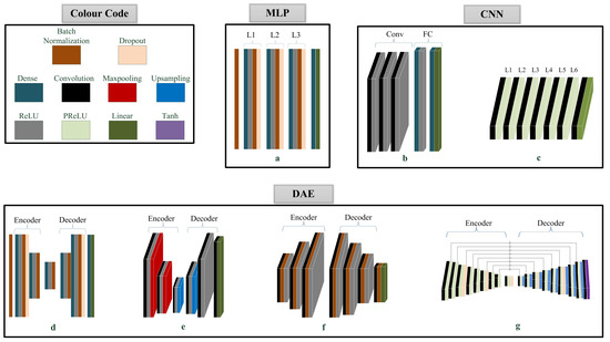
Figure 2.
The seven DNN-based speech enhancement architectures: (a) MLP, (b) the basic CNN, (c) the FCNN, (d) the DDAE, (e) the basic CDAE, (f) a special type of CDAE, and (g) the deep CDAE.

Table 1.
The configuration of the seven implemented DNNs. This table represents the different types of layers used: Batch Normalization (BN), Fully Connected (FC), and Convolution (Conv). It also represents the number of units (Units), activation function (Activation), dropout ratio (Dropout), kernel size (Kernel), number of filters (Filters), and the sizes of max pooling (MP), upsampling (US), and stride.
From the first category, MLP, the basic MLP architecture [36,38] was implemented, as in Figure 2a. The architecture has three fully connected hidden layers of 2048 units and ReLU activations. Each hidden layer is followed by a batch normalization layer in order to improve performance and training stability, and 20% rate dropout layer to avoid overfitting.
From the second category, CNN, two architectures were implemented. The first is the basic CNN architecture [48,49], as in Figure 2b, and it has three 2D convolutional layers with ReLU activations, followed by two fully connected layers for predicting the output. However, we edited this architecture by removing the max pooling layers, in order to prevent information loss due to the absence of a speech reconstruction step; moreover, the removal of these layers was proven to enhance the performance [73]. The number of filters in each convolution layer was set to 64, and we used kernels of size (3 × 3) in all layers. 512 hidden units were used in the first fully connected layer with ReLU activations, while linear activations were used in the last prediction layer. The second architecture from this category is the FCNN [43], as in Figure 2c, with six 1D convolution layers with PReLU activations, and a final convolution output layer with linear activations. The used filter size was 64 and the kernel size was 20, and they are constant across all layers.
From the third category, DAE, four architectures were implemented; one DDAE architecture [55] and three CDAE architectures. The DDAE architecture, as in Figure 2d, has two fully connected layers of 2048, and 500 hidden units, respectively, in each of the encoder and decoder networks. A bottleneck fully-connected layer of 180 hidden units between the encoder and the decoder. ReLU activations and batch normalization were used in all layers, and a 20% dropout rate was used in the first layer of the encoder and the last layer of the decoder.
The second architecture, as in Figure 2e, is the basic CDAE architecture [56]. The encoder and decoder both consist of three 2D convolution layers with ReLU activations. A max pooling layer was added after every convolution layer in the encoder network, while convolution layers are followed by upsampling layers in the case of the decoder. The number of filters in each convolution layer was 64, while the max pooling and upsampling sizes were (2 × 2). ReLU is the activation function that is used in all layers, except the final convolution layer, in which a linear activation is used in order to predict the target.
The third architecture [57] is a special type of CDAE. This architecture, as in Figure 2f, has three 2D convolution layers in each of the encoder and decoder circuits. However, no max pooling and upsampling layers were used in this architecture, in order to decrease the number of layers and prevent information loss. This network operates by increasing the filter size across the encoder network; 64, 128, and 256 filter sizes were used, and decreasing the kernel sizes; seven, five, and three kernel sizes were used. Afterwards, the reverse filter and kernel sizes were used in the decoder network. Batch normalization is used in all layers for training stability. Consequently, another feature extraction method is addressed in this network, which is the increase of the number of filter through convolution layers, instead of the bottleneck feature extraction method using max pooling layers, which was addressed in the previous architecture. This will be the main factor affecting the performance of this architecture when compared to other similar architectures.
The final architecture [58,65] is also a CDAE, as in Figure 2g, and it combines all of the techniques that were addressed in the previous three CDAE networks, in addition to the effect of 1D strided convolutions and increased depth. This network has nine 1D convolutional layers with PReLU activation functions in the encoder and decoder, and a final convolution output layer of TanH activations. Strided convolutions of size 2 were used in the encoder network, while upsampling was used in the decoder. Every three successive layers have the same filter and kernel size. The filter size increases after every three hidden layers; 64, 128, and 256 filter sizes were used, while the kernel size decreases; seven, five, and three kernel sizes were used. A dropout layer of rate 20% was included after every three layers in order to overcome overfitting. Skip connections are added to this architecture in order to avoid information loss that might occur as the processing proceeds deeper through the network.
The chosen architectures are from the best performing models belonging to the three main categories under investigation. Referring to Figure 2 and Table 1, the setup of these models was chosen in order to fairly compare specific features that are unique for each architecture type.
For the fully-connected architectures, a and d, it is clear that the configuration of both architectures is the same, the difference in architecture d is a decrease in the number of hidden nodes and the addition of a decoder network for audio reconstruction. Therefore, architecture d is an autoencoder version of architecture a, and it will show the effect of autoencoder related operations when compared to architecture a. The same applies to the convolution-based architectures, b and e. Architecture e is an autoencoder version of b, by removing the fully-connected layers and using max pooling layers, for dimensionality reduction, and a decoder network for audio reconstruction.
For the CNN architectures, b and c, architecture c is a FCNN version of b. The main differences between these architectures are: replacing the fully connected layers with convolutional layers, the processing the audio while using one-dimensional (1D) convolutions instead of 2D, and using PReLU activations instead of ReLU. The effect of these three factors will be separately discussed in the Results section.
Regarding the CDAE based architectures, the difference between architectures e and f is the feature extraction method, because architecture e is based on max pooling layers, while architecture f is based on increasing the number of filters through the hidden layers without max pooling layers. Consequently, feature extraction is the point of comparison here. Finally, architecture g addresses the use of 1D strided convolutions for DAEs and the effect of increasing the depth with the use of skip connections.
4. Experimental Setup
4.1. Dataset Selection
There are many training datasets found in the literature for speech, noisy speech, and noise. Table 2 provides a review of these datasets. In this work, we used the most commonly used datasets for speech enhancement that were available online. Three clean speech datasets were used: the Voice Bank corpus [74], LibriSpeech corpus [75], and the 176 Possible Languages corpus [76]. Five hours of clean English speech was randomly selected from the Voice Bank corpus to be used in the training process of the DNNs, while, for testing purposes, 30 min. of clean speech, not seen in the training process, was selected from the same corpus. The other two clean speech corpora were used in order to test the generalization ability of the networks, so another 30 min. of clean speech was selected from each. The 30 min. of speech from the 176 Possible Languages corpus contains 90 different languages. It should be noted that five hours of clean speech is enough for the architectures to converge, and no significant improvement was found when increasing the training dataset size, based on practical trials.
On the other hand, different noise environments were used for training and testing purposes. In the training process, a total of 105 noise environments were selected from two corpora: 90 from the 100 Environmental Noise corpus [77] and 15 from the NOISEX-92 corpus [78]. In order to test the effect of increasing the number of noise environments used in the training procedure, further noise environments were selected from the ESC 50 dataset [79], Urban Sound dataset [80], and DEMAND Dataset [81], to make a total of 1250 different noise environments. In the testing process, 20 noise environments were used, half-seen and half-unseen in the training process. These noise environments are a mixture of human-generated noise, such as crying, yawning, and human crowd sounds; and, other non-human generated noise, such as Additive White Gaussian Noise (AWGN), phone dialling, shower noise, tooth brushing, and wood creaks. Figure 3 represents the spectrograms of the noise environments that were used in the testing process. This figure shows how these noise environments are varying and challenging, which proves that the evaluation and obtained results in this work are non-biased.
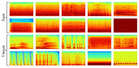
Figure 3.
Spectrograms of the noise environments used in the testing process.
In order to evaluate the networks’ performance in challenging conditions, an online dataset for reverberant speech was used [82], and babble noise audio files were taken from this online dataset [83]. The Lombard GRID corpus [84] was used while investigating the effect of Lombard phenomena.
Table 2.
A review of the available speech, noisy, and noise datasets.
Table 2.
A review of the available speech, noisy, and noise datasets.
| Corpus | Description |
|---|---|
| Clean Speech Datasets | |
| TIMIT | English speech recording for 630 speakers, 10 sentences for each speaker, sampled at 16 kHz [85] |
| Voice Bank | English speech recording for 500 speakers, 400 sentences for each speaker, sampled at 48 kHz [74] |
| LibriSpeech | 1000 h of read English speech, sampled at 16 kHz [75] |
| ATR | 16 h of English speech, sampled at 48 kHz [86] |
| TED-LIUM | 118 h of English speech recorded from TED talks, sampled at 16 kHz [87] |
| WSJCAMO | 140 speakers each speaking about 110 British English utterances, all sampled at 16 kHz [88] |
| Free ST | 350 English utterances for 10 speakers, sampled at 16 kHz [89] |
| 176 Spoken Languages | 12,320 different Speech Files, each containing approximately 10 s of speech recorded in 1 of the 176 Possible Languages Spoken, sampled at 16 kHz [76] |
| Lombard GRID | A total of 5400 utterances, 2700 utterances with Lombard effect and 2700 plain reference utterances, spoken by 54 native speakers of British English [84] |
| Noisy Speech Datasets | |
| AMI | 100 h of real meeting recordings in three different rooms with different acoustic properties. These recordings include close-talking and far-field microphones, individual and room-view video cameras [90] |
| Reverberant | An artificial reverberant speech version of the Voice Bank clean speech corpus [82] |
| Voice bank | Noisy version of the Voice Bank clean speech corpus, created by artificially adding real noise to the speech [74] |
| Noise Datasets | |
| NOISEX-92 | Recording of various noises including: babble, factory, HF channel, pink, white, and military noise [78] |
| UrbanSound8K | 8732 recordings of 10 urban noises including: air conditioner, car horn, children playing, dog bark, drilling, engine idling, gunshot, jackhammer, siren, and street music [80] |
| Baby Cry | About 400 different recordings of different baby cry sounds [91] |
| Demand | A collection of multi-channel recordings of acoustic noise in diverse environments including: park, office, cafe, and street [81] |
| ESC 50 | A collection of 2000 recordings for 50 environmental noises, 40 for each, including: animal, nature, and urban sounds [79] |
| CHiME3 | 4 noise environments including: cafes, street junctions, public transport (buses), and pedestrian areas [92] |
| USTC | 15 home noise types including: AWGN, babble, car, and musical instruments sounds [93] |
| 100 Noise | 100 non speech environmental sounds including: wind, bell, cough, yawn, and crowd noise [77] |
4.2. Training Setup
The speech signal is corrupted by the training noise environments at 0 dB SNR in order to create the training noisy speech. The training data are then normalized to zero mean and unit variance to facilitate the training process. The input audios were downsampled to 8 kHz to feed the network with the most relevant band of frequencies, and a Hamming window of frame length 32 ms (256 samples) with 50% overlap was used. The magnitude power spectrum of the signal was then extracted with 256 FFT size, and the noisy phase was kept to be added to the estimated clean speech, while assuming that the phase is less affected by the noise [94]. Magnitude spectrogram mapping is the training target used in all evaluations in order to ensure the good generalization for all architecture types [32].
The seven DNN architectures, as discussed in Section 3, were implemented while using the Keras library with Tensorflow backend. Minimum Mean Square Error (MMSE) is the loss function that is used during the training process as the default choice, because our goal here is to improve all of the evaluation metrics, not a specific one [33]. The Adam optimizer was used; learning rate = 0.001, 1 = 0.1, 2 = 0.999. A batch size of 128 was used, and 10% of the training data was used in validation in order to monitor the performance of the networks, to avoid overfitting. For all DNNs, no improvement in the performance was detected after 40 epochs, so the training process of all architectures is based on 50 epochs.
5. Results and Discussion
In this section, the results will be presented, followed by explanations and critical discussion. The experiments are divided into two parts. Part 1 aims to show the effect of the DNN model on the performance through a comprehensive analysis of the seven DNNs while using five objective metrics, a subjective test, an evaluation in challenging noise environments, testing the generalization ability, and analyzing the networks’ complexity and processing time. Furthermore, the investigation of network-related hyperparameters is considered. Additionally, Part 2 is an examination of the effect of some data structure related factors, such as the Lombard effect and the dataset preprocessing effect. The presented results and conclusions are based on a variety of architectures, noise environments, and evaluation methods; for the conclusions to be as generalized as possible.
5.1. Objective Evaluation
Table 3 shows the results of the five standard, commonly used speech enhancement objective measures: Perceptual Evaluation of Speech Quality (PESQ) [95], Short Time Objective Intelligibility (STOI) [96], Log Spectral Distortion (LSD) [97], Signal to Distortion Ratio (SDR) [98], and Segmental Signal to Noise Ratio difference (ΔSSNR) [99], for the seven implemented architectures. The results are based on the average of three high SNR levels: 20 dB, 15 dB, and 10 dB; and three low SNR levels: 5 dB, 0 dB, dB. The average of low and high SNRs is also provided in the table and it is shown for PESQ and STOI scores in Figure 4.
Table 3.
PESQ, STOI, LSD, and, ΔSSNR results at high SNR levels: 20 dB, 15 dB, and 10 dB; low SNR levels: dB, 0 dB, 5 dB; and, the average of high and low SNRs (ave).
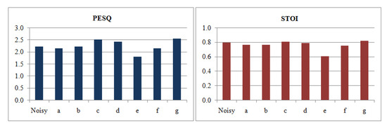
Figure 4.
Average PESQ and STOI results for the seven DNNs at six SNR levels.
The MLP network, a, generated clean speech with good overall perception concerning all of the evaluation metrics, in the case of low SNRs, as compared to the basic CNN network, b. However, network b performs better at high SNR levels. Furthermore, an enhancement in the overall performance of MLP-based networks can be achieved using bottleneck features, such as in the DDAE, d. The FCNN, c, performs better than the fully-connected networks, a and d, especially in terms of speech intelligibility (STOI). Regarding CDAE networks, e, which is the basic autoencoder version of network b, generates speech with the poorest overall performance. However, increasing the number of filters through the hidden layers and removing max pooling layers, such as in the CDAE network, f, results in a better overall performance. Additionally, a significant enhancement in the overall performance is achieved in the case of increasing the depth of the architecture and the use of 1D strided convolutions, such as in the case of the deep CDAE, g.
It is also clear that most of the networks are not enhancing the noisy speech at high SNR, especially for STOI; moreover, the average results of the noisy speech are better than the processed speech for some networks, such as a, b, e, and f, and this is due to the effect of DNN de-noising processing, which negatively affects the output speech quality, and it results in worse performance than the noisy version at high SNRs.
The spectrograms shown in Figure 5 show the clean, noisy, and estimated speech from the seven DNNs when tested while using noisy speech with tooth brushing unseen noise at 0 dB SNR. All of the models managed to remove most of the background noise and output enhanced speech with some remaining noise, highlighted with the dashed black line. The output speech from all of the networks also suffers from distortion, highlighted with the solid black line. The amount of distortion and residual noise are the main factors affecting the performance of each model, for example, network (a) and (e) suffer from very high distortion, and this explains why they have poor performance. Moreover, the output from network (e) experiences high-intensity noise and some distortion that affects the fundamental frequencies; for this reason, it has the poorest performance when compared to other models. Network (b–d,f) have some remaining high intensity noise that affects the fundamental frequencies of speech; however, they have less distortion when compared to network (a) and (e); consequently, they outperformed them. Moreover, network (g) is the only one that managed to mitigate the noise affecting the fundamental frequencies with a good reconstruction of the speech signal as well. Although network (f) managed to remove more noise as compared to (g), the fact that it has some residual high-intensity noise affecting the fundamental speech frequencies makes it perform worse than (g).
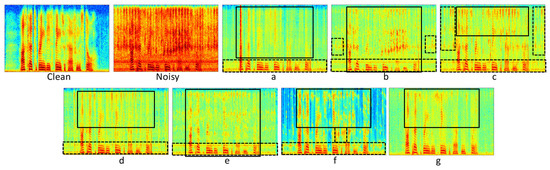
Figure 5.
The spectrograms of clean speech, its noisy version with toothbrush noise, and the output estimated clean speech from the seven DNNs. Solid black and dashed lines highlight high distortion and high intensity residual noise, respectively.
5.2. Subjective Evaluation
A subjective speech quality test was performed while using 23 volunteer listeners with no hearing issues. The listeners were asked to listen to enhanced speech produced by the seven DNNs, and to the noisy one. They were asked to give a score ranging between 1 and 5 for each sound file, based on the quality of the heard speech; higher values indicate better noise removal with understandable speech. The speech that was used in this test was corrupted in order to consider a variety of challenging conditions. The noisy audio consists of two English speakers, one male and one female, with two different background noise, one seen and one unseen by the networks during training. The noises used are human-generated non-periodic crowd noise and non-human generated periodic phone dialling noise. The noise and speech intensity are kept the same, so this evaluation is based on 0 dB SNR.
Table 4 shows the statistical analysis of the obtained results. The average (Ave) and the Standard Deviation (SD) were first calculated. It is noticed that network c is the best performing based on the human listeners’ opinion, not g, as shown before by the objective evaluation. The reason for this mismatch is the different preferences of listeners, because some listeners may prefer the existence of some remaining noise with a clearer speech, such as in the case of network c rather than removing most of the background noise with non-perfect speech reconstruction, as in the case of network g, while a computer algorithms output is negatively affected by any residual noise. Consequently, although the compression process in DAEs and depth of the architecture help in removing the noise, it may have a negative impact on the quality of the heard speech. The listeners’ different preferences are also proven by the high SD in the case of the noisy speech, because some listeners seem to find the noisy speech version better than the processed clean speech, because the enhanced speech from any DNN experiences a level of distortion, which affects speech intelligibility. The mode was then calculated in order to show the score value with the highest occurrence among listeners for each architecture, and the percentage of occurrence of this score was also calculated. This also shows that most of the listeners preferred the processed speech by network c. Moreover, the original noisy speech and network (e) have the lowest score, the same as reported by the objective evaluation. Finally, the P-value was calculated to show the significance of the results as compared to the noisy speech, the two-tailed T-test was performed with a 95% confidence level. It was found that there is no significant difference between the average scores of network (a) and (e) when compared to the noisy speech, and this is due to the high distortion of these networks, as shown in Figure 5. The same test was also performed between all combinations of architectures, and the results show that there is no significant difference between network (d) and (g), and network (b) and (f).
Table 4.
Subjective evaluation results.
5.3. Evaluation in Challenging Conditions
Although deep learning-based speech enhancement is proven to be very efficient in generating clean speech with relatively high quality and intelligibility, some noise environments are still considered to be very difficult for a DNN to deal with. Figure 6 shows the effect of three challenging noise environments: speech babble noise (N1), having two noises in the background instead of one (N2), and reverberant speech (N3). These results are based on testing the seven architectures at six SNRs from to 20 with a step of 5, and then the average was calculated.
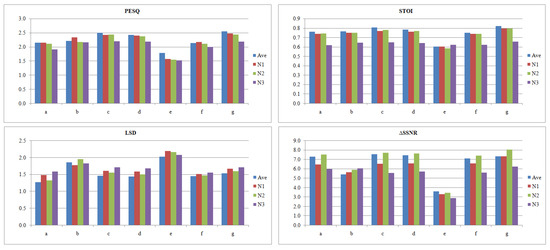
Figure 6.
PESQ, STOI, LSD, and ΔSSNR results for three challenging noise environments: babble noise, N1; two background noises, N2; and reverberation, N3; compared to the average of seen and unseen noise shown in Table 3, Ave.
It is clear that there is a degradation in the performance of all the architectures in the cases of speech babble noise and having two noise environments. However, architecture g is still the best performing architecture, and the negative effect is acceptable in most of the architecturesm as the output speech is still of quite good quality and intelligibility, except for architecture e, which was originally producing a bad performance. It should also be noted that network b shows a good generalization for the speech babble noise environment concerning all evaluation metrics, excluding STOI. Moreover, all of the networks have high ΔSSNR for two noise environments, which is logical due to the removal of more noise. Regarding reverberant speech, there is a significant negative impact on the performance of all networks, especially the intelligibility of the output speech (STOI). Based on these results, it can be interpreted that reverberation is the most challenging environment for DNNs; consequently, reverberation can be considered to be an extra task for the DNN besides the de-noising task. A solution to this issue is to train the DNN to output de-noised reverberant speech in the case of reverberation [37], and then de-reverberation can be performed as a second stage if needed.
5.4. Evaluation of the Generalization Ability
A common problem of deep learning-based speech enhancement is having a network that performs well on the training dataset; however, it is unable to generalize and maintain the same good performance for unseen data. This problem is technically known as variance or the overfitting problem. Consequently, testing the generalization ability of the networks is crucial for making a fair comparison between them. The generalization ability of the seven implemented DNNs was evaluated by testing the networks’ performance under three mismatched conditions: unseen noise environments (C1), the unseen LibriSpeech English speech dataset (C2), and unseen 90 different languages (C3). These results, as shown in Figure 7, were generated by testing the DNNs on six SNRs that ranged from to 20 with a step of 5, and then the average was calculated.
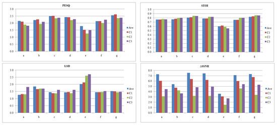
Figure 7.
PESQ, STOI, LSD, and ΔSSNR results for the processed unseen noisy speech from the same training dataset, C1; from unseen dataset, C2; and, speech from 90 different languages, C3, as compared to the average results shown in Table 3, Ave.
Most of the architectures maintained good performance in the case of unseen noise and speech from the same training dataset, C1. However, a remarkable deterioration in the performance happened for the other two mismatched conditions, unseen dataset, C2, and unseen language, C3, concerning all of the evaluation metrics, except STOI. However, architecture f shows a very good generalization ability in the case of using different languages, and this proves the power of extracting speech features by increasing the number of filters through the convolutional layers, which is the specific property of this architecture. An explanation of the increase in the STOI score in the case of these mismatched conditions is that the network does not harshly remove noise, as shown in the ΔSSNR results, so this results in more intelligible speech. This shows a tradeoff between noise removal and speech intelligibility and it gives a reason why DNNs output speech with lower STOI than the noisy version at high SNRs, as discussed in Results Section 5.1 and shown in Table 3.
5.5. Complexity Comparison
DNNs are generally complex and they have huge computational costs. Analyzing the complexity of the network is very important in evaluating its applicability in a real-time implementation, as complex architectures might not fit onto the device hardware, such as mobile devices and hearing aids. Moreover, the complexity of the network increases the processing time, which is another factor limiting the network applicability. A complexity comparison was carried out between the seven speech enhancement DNNs by looking into the three factors that are related to network complexity: the number of parameters, number of layers, and processing time. Table 5 provides this comparison.
Table 5.
Comparing different networks’ parameters: number of network parameters (Parm.) and layers (Layers), and testing processing time (time).
The number of parameters for the fully connected architectures (a and d) is very high, while convolutional-based architectures: b, c, and e have a much lower number of parameters. Although architecture f is a convolution-based network, the increased number of parameters is due to increasing the number of filters through the hidden layers. It is the same for architecture g, besides the deep nature of this network. The processing time was calculated by processing 224 speech audio files of approximately 15 min. duration in total. The algorithm was running on an NVIDIA Quadro M3000M GPU with clock 1050 MHz and 160 GB/s memory bandwidth. The processing time is inversely proportional to the depth of the architecture, which is represented by the number of layers. It also depends on the architecture type, as convolutional-based DNNs are faster. Overall, architecture b is the least complex concerning of the metrics presented in Table 5, since it is a CNN shallow network.
Figure 8 shows the loss curves of the training and validation data for the seven architectures during the training process in order to show how the complexity and type of network affect the training process. It can be seen that the fully-connected architectures, (a) and (d) converge the fastest, as the high number of parameters and connections between hidden nodes enables the network to learn speech features faster. The same fast converging behaviour can be seen with the convolutional network (f) and that shows the power of increasing the number of filters through the hidden layer in extracting the features. The other convolution-based DNNs (b), (c), (e), and (g) show a more smoothly decreasing loss curve. Although these DNNs take a longer time for the learning curve to saturate, some of them end up with a better performance, such as architectures (c) and (g).
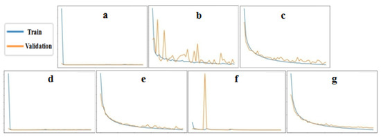
Figure 8.
The training loss curves of the seven DNNs for the training and validation data.
5.6. Network Related Hyperparameters Effect
5.6.1. MLP Architectures
Many experiments were found to show the effect of different factors on the performance of MLPs; for this reason, we did not perform experiments on this architecture. In Reference [36], the effect of the depth of the network was investigated, and it was proved that increasing the depth leads to improved performance. However, in the same work, the performance decreased if the MLP became too deep, because the network starts to overfit to the training data. The study presented in [100] shows that the more hidden units the better the performance; as a result, the number of neurons with an acceptable performance should be selected, using the trial and error approach, to decrease computational cost and complexity whilst maintaining reasonable performance.
5.6.2. CNN Architectures
ReLU is the most common activation function used today, which outputs zero if the input is negative and gives the input value for a positive input. ReLU was found to be the most similar function to the non-linearity computations in biological neurons and it proved to produce a better performance [13,101]. Moreover, ReLU has been proven to solve the vanishing and exploding gradient problem for DNNs [102]. However, a negative effect of ReLU, known as Dying ReLU [11], occurs when the ReLU neurons became inactive and output zero for any given input. LReLU, ELU, and PReLU are edited versions of ReLU that give a small value output for a negative input instead of zero, to overcome the Dying ReLU problem. Table 6 provides the effect of changing the activation function from ReLU to its edited versions for the CNN architecture b, which results in PReLU being the best performing activation function concerning all evaluation metrics.
Table 6.
Effect of CNN related hyperparameters: activation functions, e Rectified Linear Unit (ReLU) (CNN(b)), Leaky ReLU (LReLU), Exponential Linear Unit (ELU), and Parametric ReLU (PReLU); increasing filters and kernel sizes in hidden layers; the use of one-dimensional (1D) convolutions.
In order to understand how CNNs deal with the speech enhancement problem and show the effect of changing the activation function, a visualization to the spectrograms of the hidden layers is shown in Figure 9, Figure 10, Figure 11 and Figure 12. Figure 10 represents 32 filters and their activations for the first hidden layer of network b, where the ReLU was used. The figure shows the output of the network tested while using noisy speech (N) and its corresponding clean one (C), in order to show the behaviour of the network in both cases. It was noticed that CNNs manage to solve the speech enhancement task by applying a set of filters; these filters are separately represented in Figure 9 and described in the Table 7, below it. Some of the filters are responsible for the de-noising process, such as f1, which mitigates the noise and outputs enhanced speech. f2 is also a de-noising filter; however, this filter attempts to enhance the speech signal by smoothing the noise intensity in order to highlight speech and then outputs enhanced speech with the same intensity noise. Another interesting filter is f3, which works the same way as f2; however, the output of this filter is noise, so it acts as a noise detector. Other types of filters are responsible for extracting speech features, such as f4, which acts as a bandpass filter that outputs high and low speech frequency components. It was also found that there is a kind of filter that acts as a buffer, such as f5, which does not affect the original input signal. This filter is suggested to help the network in reconstructing the clean speech and avoid the loss of essential information. Figure 11 shows randomly selected filters and their activations from the second and third hidden layers of the same network; it was noticed that the same set of filters also exists in these layers, with an extra filter f6 that acts as a high pass filter that outputs the high-frequency speech components.
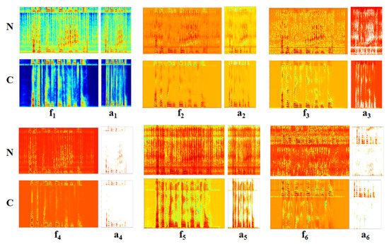
Figure 9.
Six spectrograms randomly selected from the hidden layers of network b, explaining the different Convolutional Neural Network (CNN) filters for speech enhancement, for a processed noisy speech (N) and its clean version (C), f and a represent the convolution filters and activations, respectively.
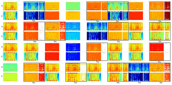
Figure 10.
The spectrograms of 32 randomly selected convolution filters (wider spectrogram) and ReLU activation outputs from the first hidden layer of the CNN architecture b, for a processed noisy speech (N) and its clean version (C), f represents convolution filters, a represents activations.
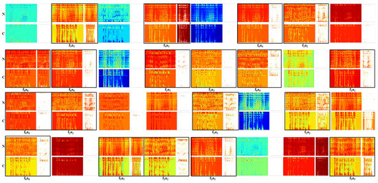
Figure 11.
The spectrograms of 32 randomly selected convolution filters (wider spectrogram) and ReLU activation outputs from the second and third hidden layers of the CNN architecture b, for a processed noisy speech (N) and its clean version (C), f represents convolution filters, a represents activations.
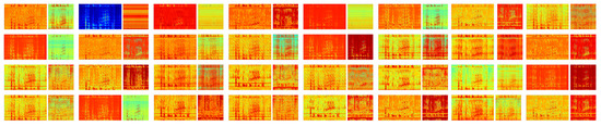
Figure 12.
The spectrograms of 32 randomly selected convolution filters (wider spectrogram) and the PReLU activation outputs for the first hidden layer of the CNN architecture b, for a processed noisy speech.
Table 7.
Description of CNN filters for the speech enhancement task.
The dying ReLU problem is clear in Figure 10 and Figure 11, as ReLU is turning off many filters, empty (white) diagrams. However, this problem was not detected when visualizing the network hidden layers when using PReLU, as show in Figure 12. This is a reason why PReLU outperforms ReLU; it can be seen from this visualization that the output after PReLU is either an enhanced speech signal or noise.
Referring to Table 6, “filters” and “K5×5” columns, the effect of increasing the filters through hidden layers is also addressed by using 64, 128, and 256 filters in the first, second, and third layers, respectively, instead of fixing the number of filters to 64. This has a positive impact on the overall performance of the network. Moreover, a kernel of size (5 × 5) was used instead of (3 × 3) in order to show the effect of increasing the kernel size, and it can be seen that this also has a positive impact on the performance. Finally, 1D convolutions with PReLU were used, instead of 2D with ReLU, with a kernel size of 20. A remarkable enhancement is shown in this case, as compared to the original CNN network, b. The implemented network after applying these modifications, (CNN1D) shown in Table 6, reached a performance closer to network c and g. Moreover, this network was included in the subjective testing, as in Section 5.2, and it obtained an average score of 3.87, with 0.81 SD. Additionally, the output of the T-test shows that there is no significant difference between the average of this model and network c.
5.6.3. DAE Architecture
Table 8 shows the results of the experiments for DAEs. The effect of depth was investigated; moreover, the function that was used for dimensionality reduction and the factors that affect CNN architectures, as discussed above, were investigated. The results refer to DDAE (d), and a deeper version of it, ddeep, with two more layers in each of the encoder and the decoder. The number of hidden nodes used are: 2049, 1024, 500, 250, and 180. Increasing the depth of DDAE was found to degrade the performance due to network overfitting, as in the case of the MLP. However, another reason for this degraded performance is the compression in the bottleneck layer, which may result in a loss of information for deep networks. The use of skip connections is a solution to this issue, although the effect of them was not investigated in our work for the DDAE, it was proven to improve the performance [41].
Table 8.
Effect of Denoising Autoencoder (DAE) related hyperparameters: increasing the depth ddeep and edeep; the use of strided convolutions, estrided; and, the use of one-dimensional (1D) strided convolutions with PReLU eedited.
The basic 2D CDAE network, e, was edited by using strided convolutions instead of max pooling, estrided. It can be noticed that strided convolutions lead to better results. Afterwards, the use of strided 1D convolutions with PReLU and increasing the number of filters through the hidden layers were considered, network eedited, which results in further enhancement in the performance, as proven in the previous subsection. Finally, one more layer was added to each of the encoder and the decoder to show the effect of increasing the depth, as shown in edeep. It can be concluded that increasing the depth of CDAE models results in a significant gain in the performance.
5.7. Lombard Effect
In real conditions, the speakers normally raise their voices in noisy environments in order to increase speech intelligibility, the phenomena known as the Lombard Effect [103]. In order to address the effect of this phenomena on the implemented DNNs, an audio-visual Lombard speech corpus [84] was used, which contains 5400 utterances, 2700 Lombard, and 2700 plain reference utterances, spoken by 54 native speakers of British English. A testing duration of 30 min. of speech, the same as the one used in the previous evaluation, was selected from each of the Lombard and plain speech audios, and then these audios were corrupted by the same 10 unseen noisy environments used before, at the same SNR levels. All the DNNs in Figure 2 were tested using these data, and the average of the results was calculated, as shown in Table 9.
Table 9.
Average results for PESQ, STOI, LSD, and ΔSSNR when testing the seven DNNs using plain (P) and Lombard effect simulated speech (L) at six SNR levels, from to 20 with a step of 5.
The Lombard effect simulated speech results with better speech intelligibility for all of the tested DNNs and better overall performance for most of the architectures. Although the Lombard effect simulated speech is considered to be unseen data to the DNN, it results in improved speech intelligibility. Based on this fact, it can be concluded that DNNs are reacting in the same way as the human brain to this phenomena and the learned features during the training process made the network robust to the change in the speech features that result from this phenomena. These results also support what was reported in [104]; however, here, the authors trained a DNN while using Lombard simulated speech, and it was proven to result in a better performance than training the network with normal speech.
5.8. Dataset Preprocessing Effect
DNN-based speech enhancement is a data-driven approach, so having a good architecture is not the only factor to achieve better performance. The dataset used in the training procedure and how these data are prepared before being fed to the network are other factors that have an impact on the network output. The effect of the training dataset was investigated while using the four best performing DNN speech enhancement networks from each category: a, d, g, and the modified better performing architecture CNN1D, as discussed in Section 5.6. It is shown how the networks’ performance is affected by three factors, the input sampling frequency, the training SNR, and the number of training noise environments. Figure 13 shows the results of these experiments.
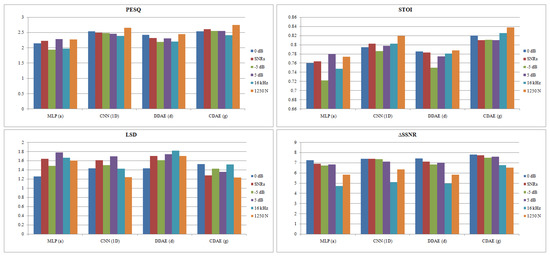
Figure 13.
PESQ, STOI, LSD, and ΔSSNR results when training the network at different SNR levels, when using sampling frequency 16 kHz instead of 8 kHz, and when increasing the number of noise environments to 1250 instead of 105.
Regarding the effect of the training SNR, training the DNN at 0 dB SNR leads to the best performance concerning all of the evaluation metrics at the tested SNR levels (−5 to 20 with a step of 5). However, architecture a shows a higher PESQ and STOI score in the case of training the network with high SNR (5 dB), but the other metrics are negatively affected. Therefore, the noise and speech intensity level is an important feature that the DNN looks at in the training process, so it is recommended to work at 0 dB as the default SNR, or try a range of SNRs and choose the best, depending on the evaluation metric with the highest priority to improve, and the real-time testing conditions.
Concerning the effect of the down-sampling operation, it can be noticed that all of the architectures output speech with better quality and higher ΔSSNR when trained using 8 kHz audio. Furthermore, the fully-connected-based DNNs (MLPa, DDAEd) perform better when using the 8 kHz sampling frequency with respect to all of the metrics. However, convolution-based architectures (CNN1D, CDAEg) output speech with a slightly higher intelligibility score and lower distortion when operating in the 16 kHz sampling frequency. It should be mentioned that 8 kHz processing outperforms in terms of the de-noising task; however, when listening to the enhanced audios, although the noise in the enhanced 16 kHz speech is more audible, the quality of the speech signal is better.
In the final experiment, the DNNs were trained with 1250 noise environments instead of 105. Increasing the number of noise environments has a positive impact on output speech quality and intelligibility. However, the results also show that exposing the network to a larger number of noise environments during the training process may have a negative impact on speech distortion (LSD) and the network’s ability to remove noise (ΔSSNR). This is due to increasing the network’s generalization ability to a large range of noise environments, which decreases its ability to remove noise. However, this helps the network to better learn clean speech features and, hence, output speech with better PESQ and STOI scores.
6. SWOC Analysis
In this section, a SWOC analysis will be presented for deep learning-based speech enhancement in order to highlight its Strengths, Weaknesses, Opportunities, and Challenges, to finally determine the position of the technique in the field. This is a general analysis to DNN based speech enhancement, to identify the strength of this technique and why it is a hot topic. It also defines, through weaknesses and challenges, the current issues of the technique and what research points need further investigation. While, opportunities suggest the ideas that will result in further improvements in the research area. Figure 14 shows the SWOC matrix.
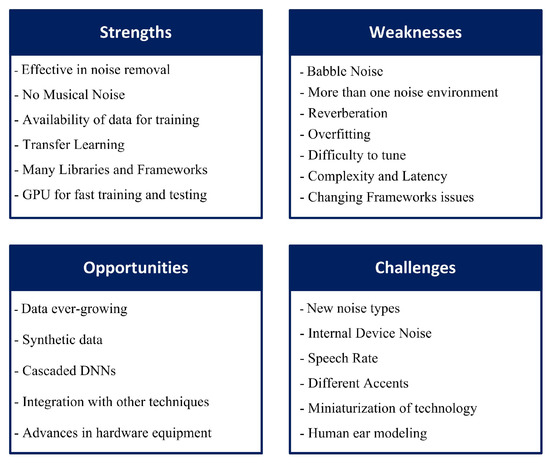
Figure 14.
SWOC Matrix.
6.1. Strengths
Regarding performance, as compared to the classical techniques, deep learning-based speech enhancement has a much greater ability to remove the noise that is accompanied with the target speech signal, even at a very low SNR. The technique is also able to output speech with good quality and intelligibility. Furthermore, the well-known problem of musical noise [105] for the classical techniques, especially the spectral subtraction method, is not present in deep learning-based methods. This is a real advantage of this approach, as the musical noise problem results in unsatisfactory performance for customers who use devices, such as hearing aids, when classical speech enhancement techniques are applied [106].
Concerning the training procedure of DNNs, which requires a huge amount of data to better predict the clean target speech, the datasets that are available online have massively increased over the previous decade, and there are many clean and noisy speech data available nowadays that can be used in the training process. Moreover, the idea of transfer learning [107] makes the technique more powerful, which is based on the reuse of a network originally trained with a huge amount of data for a certain task as a starting point to another task. Afterwards, the network is tuned with a small amount of data in orderto perform the new task, so the collection of a huge dataset is not always necessary [108].
From the implementation aspect, there are many deep learning libraries and frameworks available nowadays that make development much easier [109]. Additionally, GPU-based hardware equipment is readily available now, which leads to faster network training and real-time testing.
6.2. Weaknesses
Regarding performance, although some deep learning-based speech enhancement techniques managed to remove approximately all of the noise in the speech signal, the algorithm cannot effectively deal with interference or babble noise, which is another speech signal interfering with the target one. Most of the architectures show a degradation in the performance when tested while using babble noise, since this de-noising technique is based on learning speech features in general without having the ability to separate different speech sources. Furthermore, most evaluations of deep learning-based speech enhancement techniques in the literature are based on testing the technique using only one background noise; however, a speech signal in the real world is typically accompanied with more than one noise environment. This will make the de-noising process more challenging, leading to a poorer performance than the one that was reported with one background noise, as shown here in this work. Reverberation was also proven to be a very challenging noise environment that has a significant negative impact on the performance of all DNN architectures.
Concerning the training process, overfitting is a common problem in deep learning-based techniques, which decreases the network generalization ability. Overfitting arises from the fact that deep learning is a data-driven approach, so, the more the algorithm is fed with data, the better the performance. A network trained with a huge amount of data will perform very well in removing the noise from data that are similar to that used in the training process; however, it might not be able to generalize this performance on data under different conditions [110]. Additionally, as shown in this work, the training process of DNNs is sensitive to any change in the network’s parameters or data structure, which makes the training process difficult to tune.
From the implementation aspect, deep learning techniques are generally complex and of huge computational cost. This will be an obstacle when trying to implement the technique in real-time and may restrict its applicability for certain applications due to hardware and memory restrictions. Moreover, this complexity results in long processing times, which may not be suitable for some applications. Very fast GPUs can solve this issue; however, this will lead to higher product costs, thus decreasing its affordability. Finally, although deep learning frameworks make the developing process much easier, switching between frameworks may affect the performance. Consequently, it is not granted that a certain technique will perform the same if the framework is changed for real-time implementation purposes [35].
6.3. Opportunities
There has been an exponential increase of data recently, and this is expected to continue [111]. This ever-growing data will help in improving the performance of deep learning-based speech enhancement techniques, leading to better speech quality and intelligibility. Moreover, the technology of synthetic data is gaining popularity in the field of deep learning due to its proven positive impact on performance [112], as it can be used as a substitute in the case of data scarcity. Synthetic data are also solving the issues that are related to real data privacy and restricted use regulations and they provide more flexibility in manipulating data and creating challenging conditions to learn in the training process, which will finally result in improved performance [113]. The idea of cascading two or more DNNs to perform the speech enhancement task is also very promising [69,70,114], and some combinations of architectures have not been visited yet, which may lead to further improvements. The integration of deep learning and other techniques, such as reinforcement learning [72] and non-negative matrix factorization [115], is another field that opens the opportunity for enhancing the performance of deep learning techniques.
From the implementation aspect, advances in technology and hardware equipment will open the opportunity for deep learning techniques to invade the marketplace, because it will help in solving the high computation cost and latency, or long processing time problems [116].
6.4. Challenges
Noise levels are increasing due to the introduction of technology-related noise besides the normal environmental noise. The fast development in technology will lead to the invention of new machines, equipment, transportation, electronic devices, etc., with new kinds of noise that deep learning techniques might not be able to deal with. Moreover, the noise generated internally in electronic devices and machines [117] acts as another challenge to deep learning-based speech enhancement techniques in real-time implementations. These internal noises, which are rarely studied in the literature, are unpredictable and differ from one device to another, so they may have a negative impact on the performance [118]. Another challenge is the differing speech rates for different speakers, which may result in confusing patterns or features for the DNN. Additionally, different accents of a specific language are considered to be a challenging task for the technique, because this can result in different phonemes that may not exist in the target languages the network was trained on. Our brain can amend and understand these incorrect phonemes or pronunciation; however, it is not granted that a machine can properly deal with this issue.
The miniaturization of technology is another challenge to deep learning-based speech enhancement techniques [119]. Electronic devices are shrinking to be more efficient and portable; however, this trend may act as an obstacle when implementing deep learning techniques. Consequently, deep learning-based speech enhancement techniques may not cope with customers’ needs for smaller devices, because device miniaturization may negatively affect the techniques’ performance and restrict its applicability.
The field of computer modelling and simulation is progressing, in which many mathematical models are proposed to mimic certain phenomena or processes [120]. The modelling of the functionality of the human ear gained attraction a long time ago [121], and researchers are still developing more advanced models to simulate the complex functions of the human ear [122]. These models are competitors to deep learning-based speech enhancement techniques, as they are more understandable and controllable, while deep learning-based techniques are still ambiguous. Although there is a study that combines the two approaches to further enhance performance [123], developing a good model for the entire human ear physiology, or having a model that mimics some of the ear and brain sound analysis functionality, may lead to the disappearance of deep learning-based speech enhancement techniques.
7. Conclusions
In this work, we have completed an experimental analysis of three well-established speech enhancement architectures: deep MLP, CNN, and DAE, in order to better understand how these architectures deal with the speech enhancement process, and it is based on two approaches. The first investigates two factors that affect the performance: the chosen model and the structure of the data. Regarding the effect of the chosen model, an evaluation was performed to compare seven DNNs that belong to the above mentioned three main architectures, regarding speech quality using objective and subjective evaluation metrics, the change in performance in challenging noise conditions, generalization ability, complexity, and processing time. Furthermore, the effect of some network related hyperparameters was investigated. The effect of the structure of the data used was explored by showing how the performance changes by applying different preprocessing techniques to the training data, and showing the effect of a real phenomena, the Lombard effect. The second approach used in this analysis is visualization, using spectrograms in order to visualize the enhanced speech from all of the investigated DNNs, and the output from the internal layers of a CNN architecture. Finally, an overall evaluation of DNN-based supervised speech enhancement techniques was presented through SWOC analysis.
Concerning the evaluation and comparison of different architectures, the deep convolutional DAE architecture type proved to be very powerful in enhancing noisy speech, based on the objective measures; however, real listeners preferred the FCNN architecture due to the lossy nature of DAEs. However, the convolutional based DAE was only proven to be effective in the case of deep architectures, as the basic CNN and FCNN designs outperform shallow architectures. Regarding fully connected architectures, the DDAE was shown to outperform the basic MLP network. The output spectrograms support this, as some architectures were found to aggressively remove noise at the expense of the reconstruction of clean speech, which results in worse performance.
Regarding the effect of network-related hyperparameters, increasing the depth of fully connected networks results in no improvement; conversely, it leads to a worse performance due to network overfitting or the loss of essential information in the case of DDAE. For CNN architectures, PReLU was shown to outperform other activation functions, and the use of a 1D convolution with PReLU activation results in a remarkable improvement in the performance when compared to 2D convolutions and other activation functions. Furthermore, increasing the number of filters through the hidden layers and the kernel size also led to further improvement. In the case of the convolutional based DAE, strided convolution was shown to be better than the use of max pooling layers; moreover, the depth of this architecture type was proven to be the main factor affecting the performance.
The spectrograms of the internal layers of the CNN architecture with ReLU activation showed that CNNs deal with the speech enhancement task by applying filters with different functionalities. Some are de-noising, while others extract different speech features, such as the high and low-frequency components. Additionally, some filters were found to keep the original noisy speech, and they are supposed to help in the reconstruction of the estimated clean speech and avoid the loss of important information. However, the dying ReLU problem was detected in this case, which results in turning off many of these filters, and the use of PReLU instead was shown to solve this issue.
Challenging noisy environments, such as babble speech noise and the existence of more than one noise environment, negatively affect the performance of the DNNs. However, the overall performance remains acceptable. On the other hand, reverberation causes a significant negative effect on the overall performance of all DNNs, and it results in unintelligible output speech. DNNs must have extra techniques to deal with this specific type of noise environment differently from the denoising process.
Although most of the DNNs show good generalization ability, overfitting remains a problem for DNNs, even if a regularization technique, such as dropout, is applied. All of the networks experienced a degradation in their ability to remove noise when tested while using a different dataset from the one used in the training process, and when using different languages.
The complexity and processing time of the DNNs is affected mainly by the depth and type of network. Convolution based architectures are less complex as compared to fully connected ones, due to the sparsity in the connections between layers.
In real scenarios, speakers raise their voice in noisy environments. Although this pattern of speech with different acoustic features, such as pitch and rate, is considered to be an unseen condition during the training process, the DNNs performance improved. Consequently, the learned speech features enable the DNN to deal with the speech enhancement task in a way that is similar to the human brain and to be robust to these mismatched conditions.
Different preprocessing techniques for the input data were shown to affect the performance of the DNNs. Training the network at 0 dB SNR was shown to be the default choice, because maintaining the speech and noise power at the same level was an important factor in the training process for some DNNs. Additionally, downsampling the input audio to 8 kHz results in better overall performance in terms of noise removal, while the 16 kHz enhanced speech is of better quality, but more background noise exists. Increasing the number of training noise environments improves the PESQ and STOI scores of the output speech, as this increases the network generalization ability; however, it has a negative effect on the overall network ability to remove noise.
Finally, it can be concluded that many hyperparameters and factors highly affect DNN-based supervised speech enhancement, which all contribute to the overall quality of the output speech. Exploring the effect of these factors is the key to understanding the way this black box deals with the speech enhancement task and, hence, being able to improve the performance.
Author Contributions
J.W. initiated the main idea, S.A.N. added to the idea, performed the experimental analysis, and drafted the paper; C.G. provided technical support; supervision was performed by J.W., M.M. and C.G.; funding was acquired by N.C.; and all authors made revisions of the article. All authors have read and agreed to this version of the manuscript.
Funding
This work is funded by University of East London and Intelligent Voice Ltd, London, UK.
Conflicts of Interest
The authors declare no conflict of interest.
References
- Loizou, P.C. Speech Enhancement: Theory and Practice; CRC Press: Boca Raton, FL, USA, 2013. [Google Scholar]
- Hu, Y.; Loizou, P.C. Subjective comparison and evaluation of speech enhancement algorithms. Speech Commun. 2007, 49, 588–601. [Google Scholar] [CrossRef] [PubMed]
- Wang, D.; Chen, J. Supervised Speech Separation Based on Deep Learning: An Overview. IEEE Trans. Audio Speech Lang. Proc. 2018, 26, 1702–1726. [Google Scholar] [CrossRef] [PubMed]
- Ephraim, Y.; Malah, D. Speech enhancement using a minimum mean-square error log-spectral amplitude estimator. IEEE Trans. Acoust. Speech Sig. Proc. 1985, 33, 443–445. [Google Scholar] [CrossRef]
- Kwan, C.; Chu, S.; Yin, J.; Liu, X.; Kruger, M.; Sityar, I. Enhanced speech in noisy multiple speaker environment. In Proceedings of the 2008 IEEE International Joint Conference on Neural Networks (IEEE World Congress on Computational Intelligence), Hong Kong, China, 1–8 June 2008; pp. 1640–1643. [Google Scholar]
- Drullman, R. Speech intelligibility in noise: Relative contribution of speech elements above and below the noise level. J. Acoust. Soc. Am. 1995, 98, 1796–1798. [Google Scholar] [CrossRef] [PubMed]
- Loizou, P.C.; Kim, G. Reasons why current speech-enhancement algorithms do not improve speech intelligibility and suggested solutions. IEEE Trans. Audio Speech Lang. Proc. 2010, 19, 47–56. [Google Scholar] [CrossRef] [PubMed]
- Alom, M.Z.; Taha, T.M.; Yakopcic, C.; Westberg, S.; Sidike, P.; Nasrin, M.S.; Hasan, M.; Van Essen, B.C.; Awwal, A.A.; Asari, V.K. A state-of-the-art survey on deep learning theory and architectures. Electronics 2019, 8, 292. [Google Scholar] [CrossRef]
- LeCun, Y.; Bengio, Y.; Hinton, G. Deep learning. Nature 2015, 521, 436. [Google Scholar] [CrossRef]
- Sze, V.; Chen, Y.H.; Yang, T.J.; Emer, J.S. Efficient processing of deep neural networks: A tutorial and survey. Proc. IEEE 2017, 105, 2295–2329. [Google Scholar] [CrossRef]
- Pedamonti, D. Comparison of non-linear activation functions for deep neural networks on MNIST classification task. arXiv 2018, arXiv:1804.02763. [Google Scholar]
- Nair, V.; Hinton, G.E. Rectified linear units improve restricted boltzmann machines. In Proceedings of the 27th International Conference on Machine Learning, Haifa, Israel, 21–24 June 2010. [Google Scholar]
- Maas, A.L.; Hannun, A.Y.; Ng, A.Y. Rectifier nonlinearities improve neural network acoustic models. In Proceedings of the International Conference on Machine Learning, Atlanta, GA, USA, June 16–21 2013; Volume 30, p. 3. [Google Scholar]
- Clevert, D.A.; Unterthiner, T.; Hochreiter, S. Fast and accurate deep network learning by exponential linear units (elus). arXiv 2015, arXiv:1511.07289. [Google Scholar]
- He, K.; Zhang, X.; Ren, S.; Sun, J. Delving deep into rectifiers: Surpassing human-level performance on imagenet classification. In Proceedings of the IEEE International Conference on Computer Vision (ICCV), Santiago, Chile, 7–13 December 2015; pp. 1026–1034. [Google Scholar]
- Podder, P.; Khan, T.Z.; Khan, M.H.; Rahman, M.M. Comparative performance analysis of hamming, hanning and blackman window. Int. J. Comput. Appl. 2014, 96, 1–7. [Google Scholar] [CrossRef]
- Ren, M.; Liao, R.; Urtasun, R.; Sinz, F.H.; Zemel, R.S. Normalizing the normalizers: Comparing and extending network normalization schemes. arXiv 2016, arXiv:1611.04520. [Google Scholar]
- Alías, F.; Socoró, J.C.; Sevillano, X. A review of physical and perceptual feature extraction techniques for speech, music and environmental sounds. Appl. Sci. 2016, 6, 143. [Google Scholar] [CrossRef]
- Pirhosseinloo, S.; Brumberg, J.S. A new feature set for masking-based monaural speech separation. In Proceedings of the 2018 52nd Asilomar Conference on Signals, Systems, and Computers, Pacific Grove, CA, USA, 28–31 October 2018; pp. 828–832. [Google Scholar]
- Shao, Y.; Wang, D. Robust speaker identification using auditory features and computational auditory scene analysis. In Proceedings of the 2008 IEEE International Conference on Acoustics, Speech and Signal Processing, Las Vegas, NV, USA, 31 March–4 April 2008; pp. 1589–1592. [Google Scholar]
- Dave, N. Feature extraction methods LPC, PLP and MFCC in speech recognition. Int. J. Adv. Res. Eng. Technol. 2013, 1, 1–4. [Google Scholar]
- Wang, Y.; Narayanan, A.; Wang, D. On training targets for supervised speech separation. IEEE Trans. Audio Speech Lang. Proc. 2014, 22, 1849–1858. [Google Scholar] [CrossRef]
- Odelowo, B.O.; Anderson, D.V. A Study of Training Targets for Deep Neural Network-Based Speech Enhancement Using Noise Prediction. In Proceedings of the 2018 IEEE International Conference on Acoustics, Speech and Signal Processing (ICASSP), Calgary, AB, Canada, 15–20 April 2018; pp. 5409–5413. [Google Scholar]
- Wang, D. On ideal binary mask as the computational goal of auditory scene analysis. In Speech Separation by Humans and Machines; Springer: Berlin/Heidelberg, Germany, 2005; pp. 181–197. [Google Scholar]
- Srinivasan, S.; Roman, N.; Wang, D. Binary and ratio time-frequency masks for robust speech recognition. Speech Commun. 2006, 48, 1486–1501. [Google Scholar] [CrossRef]
- Williamson, D.S.; Wang, Y.; Wang, D. Complex ratio masking for monaural speech separation. IEEE Trans. Audio Speech Lang. Proc. 2016, 24, 483–492. [Google Scholar] [CrossRef]
- Erdogan, H.; Hershey, J.R.; Watanabe, S.; Le Roux, J. Phase-sensitive and recognition-boosted speech separation using deep recurrent neural networks. In Proceedings of the 2015 IEEE International Conference on Acoustics, Speech and Signal Processing (ICASSP), Brisbane, Australia, 19–24 April 2015; pp. 708–712. [Google Scholar]
- Bengio, Y. Practical recommendations for gradient-based training of deep architectures. In Neural Networks: Tricks of the Trade; Springer: Berlin/Heidelberg, Germany, 2012; pp. 437–478. [Google Scholar]
- Chen, J.; Wang, Y.; Wang, D. A Feature Study for Classification-Based Speech Separation at Low Signal-to-Noise Ratios. IEEE Trans. Audio Speech Lang. Proc. 2014, 12, 1993–2002. [Google Scholar] [CrossRef]
- Nossier, S.A.; Wall, J.; Moniri, M.; Glackin, C.; Cannings, N. A Comparative Study of Time and Frequency Domain Approaches to Deep Learning based Speech Enhancement. In Proceedings of the 2020 International Joint Conference on Neural Networks (IJCNN), Glasgow, UK, 19–24 July 2020; pp. 1–8. [Google Scholar]
- Gong, Y.; Poellabauer, C. How do deep convolutional neural networks learn from raw audio waveforms? In Proceedings of the 6th International Conference on Learning Representations, Vancouver, BC, Canada, 30 April–3 May 2018. [Google Scholar]
- Nossier, S.A.; Wall, J.; Moniri, M.; Glackin, C.; Cannings, N. Mapping and Masking Targets Comparison using Different Deep Learning based Speech Enhancement Architectures. In Proceedings of the 2020 International Joint Conference on Neural Networks (IJCNN), Glasgow, UK, 19–24 July 2020; pp. 1–8. [Google Scholar]
- Kolbæk, M.; Tan, Z.H.; Jensen, S.H.; Jensen, J. On loss functions for supervised monaural time-domain speech enhancement. IEEE Trans. Audio Speech Lang. Proc. 2020, 28, 825–838. [Google Scholar] [CrossRef]
- Smith, L.N. A disciplined approach to neural network hyper-parameters: Part 1–learning rate, batch size, momentum, and weight decay. arXiv 2018, arXiv:1803.09820. [Google Scholar]
- Bahrampour, S.; Ramakrishnan, N.; Schott, L.; Shah, M. Comparative study of deep learning software frameworks. arXiv 2015, arXiv:1511.06435. [Google Scholar]
- Xu, Y.; Du, J.; Dai, L.R.; Lee, C.H. A regression approach to speech enhancement based on deep neural networks. IEEE Trans. Audio Speech Lang. Proc. 2014, 23, 7–19. [Google Scholar] [CrossRef]
- Zhao, Y.; Wang, D.; Merks, I.; Zhang, T. DNN-based enhancement of noisy and reverberant speech. In Proceedings of the 2016 IEEE International Conference on Acoustics, Speech and Signal Processing (ICASSP), Shanghai, China, 20–25 March 2016; pp. 6525–6529. [Google Scholar]
- Wang, D. Deep learning reinvents the hearing aid. IEEE Spectr. 2017, 54, 32–37. [Google Scholar] [CrossRef] [PubMed]
- Chen, J.; Wang, Y.; Yoho, S.E.; Wang, D.; Healy, E.W. Large-scale training to increase speech intelligibility for hearing-impaired listeners in novel noises. J. Acoust. Soc. Am. 2016, 139, 2604–2612. [Google Scholar] [CrossRef] [PubMed]
- Kumar, A.; Florencio, D. Speech enhancement in multiple-noise conditions using deep neural networks. arXiv 2016, arXiv:1605.02427. [Google Scholar]
- Tu, M.; Zhang, X. Speech enhancement based on deep neural networks with skip connections. In Proceedings of the 2017 IEEE International Conference on Acoustics, Speech and Signal Processing (ICASSP), New Orleans, LA, USA, 5–9 March 2017; pp. 5565–5569. [Google Scholar]
- Luo, Z.; Liu, H.; Wu, X. Artificial neural network computation on graphic process unit. In Proceedings of the 2005 IEEE International Joint Conference on Neural Networks, Montreal, QC, Canada, 31 July–4 August 2005; Volume 1, pp. 622–626. [Google Scholar]
- Fu, S.W.; Tsao, Y.; Lu, X.; Kawai, H. Raw waveform-based speech enhancement by fully convolutional networks. In Proceedings of the 2017 Asia-Pacific Signal and Information Processing Association Annual Summit and Conference (APSIPA ASC), Kuala Lumpur, Malaysia, 12–15 December 2017; pp. 006–012. [Google Scholar]
- Deng, L.; Yu, D. Deep learning: Methods and applications. Found. Trends Signal Process. 2014, 7, 197–387. [Google Scholar] [CrossRef]
- Schmidhuber, J. Deep learning in neural networks: An overview. Neural Netw. 2015, 61, 85–117. [Google Scholar] [CrossRef]
- Kiranyaz, S.; Ince, T.; Abdeljaber, O.; Avci, O.; Gabbouj, M. 1-D convolutional neural networks for signal processing applications. In Proceedings of the ICASSP 2019 IEEE International Conference on Acoustics, Speech and Signal Processing (ICASSP), Brighton, UK, 12–17 May 2019; pp. 8360–8364. [Google Scholar]
- Kiranyaz, S.; Avci, O.; Abdeljaber, O.; Ince, T.; Gabbouj, M.; Inman, D.J. 1D convolutional neural networks and applications: A survey. arXiv 2019, arXiv:1905.03554. [Google Scholar] [CrossRef]
- Kounovsky, T.; Malek, J. Single channel speech enhancement using convolutional neural network. In Proceedings of the 2017 IEEE International Workshop of Electronics, Control, Measurement, Signals and their Application to Mechatronics (ECMSM), Donostia-San Sebastian, Spain, 24–26 May 2017; pp. 1–5. [Google Scholar]
- Chakrabarty, S.; Wang, D.; Habets, E.A. Time-Frequency Masking Based Online Speech Enhancement with Multi-Channel Data Using Convolutional Neural Networks. In Proceedings of the 2018 16th International Workshop on Acoustic Signal Enhancement (IWAENC), Tokyo, Japan, 17–20 September 2018; pp. 476–480. [Google Scholar]
- Ouyang, Z.; Yu, H.; Zhu, W.P.; Champagne, B. A Fully Convolutional Neural Network for Complex Spectrogram Processing in Speech Enhancement. In Proceedings of the 2019 IEEE International Conference on Acoustics, Speech and Signal Processing (ICASSP), Brighton, UK, 12–17 May 2019; pp. 5756–5760. [Google Scholar]
- Pirhosseinloo, S.; Brumberg, J.S. Monaural Speech Enhancement with Dilated Convolutions. In Proceedings of the INTERSPEECH, Graz, Austri, 15–19 September 2019; pp. 3143–3147. [Google Scholar]
- Vincent, P.; Larochelle, H.; Lajoie, I.; Bengio, Y.; Manzagol, P.A. Stacked denoising autoencoders: Learning useful representations in a deep network with a local denoising criterion. J. Mach. Learn. Res. 2010, 11, 3371–3408. [Google Scholar]
- Yu, D.; Seltzer, M.L. Improved bottleneck features using pretrained deep neural networks. In Proceedings of the Twelfth annual Conference of the International Speech Communication Association, Florence, Italy, 27–31 August 2011. [Google Scholar]
- Wu, Z.; King, S. Improving trajectory modelling for DNN-based speech synthesis by using stacked bottleneck features and minimum generation error training. IEEE Trans. Audio Speech Lang. Proc. 2016, 24, 1255–1265. [Google Scholar] [CrossRef]
- Lu, X.; Tsao, Y.; Matsuda, S.; Hori, C. Speech enhancement based on deep denoising autoencoder. In Proceedings of the Interspeech 2013, Lyon, France, 25–29 August 2013; pp. 436–440. [Google Scholar]
- Grais, E.M.; Plumbley, M.D. Single channel audio source separation using convolutional denoising autoencoders. In Proceedings of the 2017 IEEE Global Conference on Signal and Information Processing (GlobalSIP), Montreal, QC, Canada, 14–16 November 2017; pp. 1265–1269. [Google Scholar]
- Park, S.R.; Lee, J. A fully convolutional neural network for speech enhancement. arXiv 2016, arXiv:1609.07132. [Google Scholar]
- Pandey, A.; Wang, D. A New Framework for CNN-Based Speech Enhancement in the Time Domain. IEEE Trans. Audio Speech Lang. Proc. 2019, 27, 1179–1188. [Google Scholar] [CrossRef]
- Coşkun, M.; YILDIRIM, Ö.; Ayşegül, U.; Demir, Y. An overview of popular deep learning methods. Eur. J. Tech. 2017, 7, 165–176. [Google Scholar] [CrossRef]
- El Hihi, S.; Bengio, Y. Hierarchical recurrent neural networks for long-term dependencies. In Advances in Neural Information Processing Systems; NIPS: Denver, CO, USA, 1996; pp. 493–499. [Google Scholar]
- Chung, J.; Gulcehre, C.; Cho, K.; Bengio, Y. Empirical evaluation of gated recurrent neural networks on sequence modeling. arXiv 2014, arXiv:1412.3555. [Google Scholar]
- Sun, L.; Du, J.; Dai, L.R.; Lee, C.H. Multiple-target deep learning for LSTM-RNN based speech enhancement. In Proceedings of the 2017 Hands-free Speech Communications and Microphone Arrays (HSCMA), San Francisco, CA, USA, 1–3 March 2017; pp. 136–140. [Google Scholar]
- Huang, P.S.; Kim, M.; Hasegawa-Johnson, M.; Smaragdis, P. Deep learning for monaural speech separation. In Proceedings of the 2014 IEEE International Conference on Acoustics, Speech and Signal Processing (ICASSP), Florence, Italy, 4–9 May 2014; pp. 1562–1566. [Google Scholar]
- Xia, Y.; Braun, S.; Reddy, C.K.; Dubey, H.; Cutler, R.; Tashev, I. Weighted Speech Distortion Losses for Neural-Network-Based Real-Time Speech Enhancement. In Proceedings of the 2020 IEEE International Conference on Acoustics, Speech and Signal Processing (ICASSP), Barcelona, Spain, 4–8 May 2020; pp. 871–875. [Google Scholar]
- Pascual, S.; Bonafonte, A.; Serra, J. SEGAN: Speech enhancement generative adversarial network. arXiv 2017, arXiv:1703.09452. [Google Scholar]
- Goodfellow, I. NIPS 2016 tutorial: Generative adversarial networks. arXiv 2016, arXiv:1701.00160. [Google Scholar]
- Mao, X.; Li, Q.; Xie, H.; Lau, R.Y.; Wang, Z.; Paul Smolley, S. Least squares generative adversarial networks. In Proceedings of the IEEE International Conference on Computer Vision (ICCV), Venice, Italy, 22–29 October 2017; pp. 2794–2802. [Google Scholar]
- Pandey, A.; Wang, D. On adversarial training and loss functions for speech enhancement. In Proceedings of the 2018 IEEE International Conference on Acoustics, Speech and Signal Processing (ICASSP), Calgary, AB, Canada, 15–20 April 2018; pp. 5414–5418. [Google Scholar]
- Zhao, H.; Zarar, S.; Tashev, I.; Lee, C.H. Convolutional-recurrent neural networks for speech enhancement. In Proceedings of the 2018 IEEE International Conference on Acoustics, Speech and Signal Processing (ICASSP), Calgary, AB, Canada, 15–20 April 2018; pp. 2401–2405. [Google Scholar]
- Tan, K.; Wang, D. A Convolutional Recurrent Neural Network for Real-Time Speech Enhancement. In Proceedings of the Interspeech 2018, Hyderabad, India, 2–6 September 2018; pp. 3229–3233. [Google Scholar] [CrossRef]
- Nicolson, A.; Paliwal, K.K. Deep Learning for Minimum Mean-Square Error Approaches to Speech Enhancement. Speech Commun. 2019, 111, 44–55. [Google Scholar] [CrossRef]
- Koizumi, Y.; Niwa, K.; Hioka, Y.; Kobayashi, K.; Haneda, Y. DNN-based source enhancement self-optimized by reinforcement learning using sound quality measurements. In Proceedings of the 2017 IEEE International Conference on Acoustics, Speech and Signal Processing (ICASSP), New Orleans, LA, USA, 5–9 March 2017; pp. 81–85. [Google Scholar]
- Fu, S.W.; Tsao, Y.; Lu, X. SNR-Aware Convolutional Neural Network Modeling for Speech Enhancement. In Proceedings of the Interspeech 2016, San Francisco, CA, USA, 8–12 September 2016; pp. 3768–3772. [Google Scholar]
- Veaux, C.; Yamagishi, J.; King, S. The voice bank corpus: Design, collection and data analysis of a large regional accent speech database. In Proceedings of the 2013 International Conference Oriental COCOSDA Held Jointly with 2013 Conference on Asian Spoken Language Research and Evaluation (O-COCOSDA/CASLRE), Gurgaon, India, 25–27 November 2013; pp. 1–4. [Google Scholar]
- Panayotov, V.; Chen, G.; Povey, D.; Khudanpur, S. Librispeech: An ASR corpus based on public domain audio books. In Proceedings of the 2015 IEEE International Conference on Acoustics, Speech and Signal Processing (ICASSP), Brisbane, Australia, 19–24 April 2015; pp. 5206–5210. [Google Scholar]
- Topcoder. 176 Spoken Languages. 2017. Available online: http://www.topcoder.com/contest/problem/SpokenLanguages2/trainingdata.zip (accessed on 22 December 2020).
- Hu, G. 100 Nonspeech Environmental Sounds. 2014. Available online: http://www.cse.ohiostate.edu/pnl/corpus/HuCorpus.html (accessed on 22 December 2020).
- Varga, A.; Steeneken, H. Assessment for automatic speech recognition: II. NOISEX-92: A database and an experiment to study the effect of additive noise on speech recognition systems. Speech Commun. 1993, 12, 247–251. [Google Scholar] [CrossRef]
- Piczak, K.J. ESC: Dataset for environmental sound classification. In Proceedings of the 23rd ACM International Conference on Multimedia, Brisbane, Australia, 26–30 October 2015; ACM: New York, NY, USA, 2015; pp. 1015–1018. [Google Scholar]
- Salamon, J.; Jacoby, C.; Bello, J.P. A dataset and taxonomy for urban sound research. In Proceedings of the 22nd ACM international conference on Multimedia, Orlando, FL, USA, 3–7 November 2014; pp. 1041–1044. [Google Scholar]
- Thiemann, J.; Ito, N.; Vincent, E. DEMAND: A collection of multi-channel recordings of acoustic noise in diverse environments. In Proceedings of the Meetings on Acoustics, Montreal, QC, Canada, 2–7 June 2013. [Google Scholar]
- Valentini-Botinhao, C. Noisy Reverberant Speech Database for Training Speech Enhancement Algorithms and TTS Models; The University of Edinburgh: Edinburgh, UK, 2017; Available online: https://datashare.is.ed.ac.uk/handle/10283/2791 (accessed on 22 December 2020).
- Reddy, C.K.; Beyrami, E.; Pool, J.; Cutler, R.; Srinivasan, S.; Gehrke, J. A scalable noisy speech dataset and online subjective test framework. arXiv 2019, arXiv:1909.08050. [Google Scholar]
- Alghamdi, N.; Maddock, S.; Marxer, R.; Barker, J.; Brown, G.J. A corpus of audio-visual Lombard speech with frontal and profile views. J. Acoust. Soc. Am. 2018, 143, EL523–EL529. [Google Scholar] [CrossRef]
- Zue, V.; Seneff, S.; Glass, J. Speech database development at MIT: TIMIT and beyond. Speech Commun. 1990, 9, 351–356. [Google Scholar] [CrossRef]
- Ni, J.; Hirai, T.; Kawai, H.; Toda, T.; Tokuda, K.; Tsuzaki, M.; Sakai, S.; Maia, R.; Nakamura, S. ATRECSS: ATR English Speech Corpus for Speech Synthesis. 2007. Available online: http://www.festvox.org/blizzard/bc2007/blizzard_2007/full_papers/blz3_002.pdf (accessed on 22 December 2020).
- Rousseau, A.; Deléglise, P.; Esteve, Y. TED-LIUM: An Automatic Speech Recognition dedicated corpus. In Proceedings of the International Conference on Language Resources and Evaluation, Istanbul, Turkey, 23–25 May 2012; pp. 125–129. [Google Scholar]
- Robinson, T.; Fransen, J.; Pye, D.; Foote, J.; Renals, S. WSJCAMO: A British English speech corpus for large vocabulary continuous speech recognition. In Proceedings of the 1995 International Conference on Acoustics, Speech, and Signal Processing, Detroit, MI, USA, 9–12 May 1995; Volume 1, pp. 81–84. [Google Scholar]
- Surfingtech. Free ST American English Corpus. Available online: http://www.openslr.org/45/ (accessed on 22 December 2020).
- Carletta, J.; Ashby, S.; Bourban, S.; Flynn, M.; Guillemot, M.; Hain, T.; Kadlec, J.; Karaiskos, V.; Kraaij, W.; Kronenthal, M.; et al. The AMI meeting corpus: A pre-announcement. In International Workshop on Machine Learning for Multimodal Interaction; Springer: Berlin/Heidelberg, Germany, 2005; pp. 28–39. [Google Scholar]
- Gveres. Donate-a-cry Corpus. Available online: https://github.com/gveres/donateacry-corpus (accessed on 22 December 2020).
- Barker, J.; Marxer, R.; Vincent, E.; Watanabe, S. The third ‘CHiME’ speech separation and recognition challenge: Dataset, task and baselines. In Proceedings of the IEEE Workshop on ASR and Understanding (ASRU), Scottsdale, AZ, USA, 13–17 December 2015; pp. 504–511. [Google Scholar]
- Xu, Y. USTC-Made 15 Noise. Available online: https://pan.baidu.com/s/1dER6UUt (accessed on 22 December 2020).
- Wang, D.; Lim, J. The unimportance of phase in speech enhancement. IEEE Trans. Audio Speech Lang. Proc. 1982, 30, 679–681. [Google Scholar] [CrossRef]
- Rix, A.; Beerends, J.; Hollier, M.; Hekstra, A. Perceptual evaluation of speech quality (PESQ): An objective method for end-to-end speech quality assessment of narrow-band telephone networks and speech codecs. In Proceedings of the 2001 IEEE International Conference on Acoustics, Speech, and Signal Processing, Salt Lake City, UT, USA, 7–11 May 2001; pp. 749–752. [Google Scholar]
- Taal, C.; Hendriks, R.; Heusdens, R.; Jensen, J. An algorithm for intelligibility prediction of time-frequency weighted noisy speech. IEEE Trans. Audio Speech Lang. Proc. 2011, 19, 2125–2136. [Google Scholar] [CrossRef]
- Du, J.; Huo, Q. A speech enhancement approach using piecewise linear approximation of an explicit model of environmental distortions. In Proceedings of the Ninth Annual Conference of the International Speech Communication Association, Brisbane, Australia, 22–26 September 2008. [Google Scholar]
- Hu, Y.; Loizou, P.C. Evaluation of objective quality measures for speech enhancement. IEEE Trans. Audio Speech Lang. Proc. 2007, 16, 229–238. [Google Scholar] [CrossRef]
- Hansen, J.H.; Pellom, B.L. An effective quality evaluation protocol for speech enhancement algorithms. In Proceedings of the Fifth International Conference on Spoken Language Processing, Sydney, Australia, 30 November–4 December 1998. [Google Scholar]
- Hunter, D.; Yu, H.; Pukish III, M.S.; Kolbusz, J.; Wilamowski, B.M. Selection of proper neural network sizes and architectures—A comparative study. IEEE Trans. Ind. Inform. 2012, 8, 228–240. [Google Scholar] [CrossRef]
- Grossberg, S. Nonlinear neural networks: Principles, mechanisms, and architectures. Neural Netw. 1988, 1, 17–61. [Google Scholar] [CrossRef]
- Glorot, X.; Bengio, Y. Understanding the difficulty of training deep feedforward neural networks. In Proceedings of the Thirteenth International Conference on Artificial Intelligence and Statistics, Sardinia, Italy, 13–15 May 2010; pp. 249–256. [Google Scholar]
- Garnier, M.; Henrich, N. Speaking in noise: How does the Lombard effect improve acoustic contrasts between speech and ambient noise? J. Comput. Speech Lang. 2014, 28, 580–597. [Google Scholar] [CrossRef]
- Michelsanti, D.; Tan, Z.H.; Sigurdsson, S.; Jensen, J. Deep-learning-based audio-visual speech enhancement in presence of Lombard effect. Speech Commun. 2019, 115, 38–50. [Google Scholar] [CrossRef]
- Uemura, Y.; Takahashi, Y.; Saruwatari, H.; Shikano, K.; Kondo, K. Musical noise generation analysis for noise reduction methods based on spectral subtraction and MMSE STSA estimation. In Proceedings of the 2009 IEEE International Conference on Acoustics, Speech and Signal Processing, Taipei, Taiwan, 19–24 April 2009; pp. 4433–4436. [Google Scholar]
- McCormack, A.; Fortnum, H. Why do people fitted with hearing aids not wear them? Int. J. Audiol. 2013, 52, 360–368. [Google Scholar] [CrossRef]
- Wang, D.; Zheng, T.F. Transfer learning for speech and language processing. In Proceedings of the 2015 Asia-Pacific Signal and Information Processing Association Annual Summit and Conference (APSIPA), Hong Kong, China, 16–19 December 2015; pp. 1225–1237. [Google Scholar]
- Xu, Y.; Du, J.; Dai, L.R.; Lee, C.H. Cross-language transfer learning for deep neural network based speech enhancement. In Proceedings of the 9th International Symposium on Chinese Spoken Language Processing, Singapore, 12–14 September 2014; pp. 336–340. [Google Scholar]
- Erickson, B.J.; Korfiatis, P.; Akkus, Z.; Kline, T.; Philbrick, K. Toolkits and libraries for deep learning. J. Digital Imaging 2017, 30, 400–405. [Google Scholar] [CrossRef]
- Lawrence, S.; Giles, C.L. Overfitting and neural networks: Conjugate gradient and backpropagation. In Proceedings of the IEEE-INNS-ENNS International Joint Conference on Neural Networks. IJCNN 2000. Neural Computing: New Challenges and Perspectives for the New Millennium, Como, Italy, 27 July 2000; Volume 1, pp. 114–119. [Google Scholar]
- Dytman-Stasienko, A.; Weglinska, A. Big Data: Digital Marketing and Trendwatching; Oficyna Wydawnicza Atut: Wrocław, Poland, 2018. [Google Scholar]
- Tremblay, J.; Prakash, A.; Acuna, D.; Brophy, M.; Jampani, V.; Anil, C.; To, T.; Cameracci, E.; Boochoon, S.; Birchfield, S. Training deep networks with synthetic data: Bridging the reality gap by domain randomization. In Proceedings of the IEEE Conference on Computer Vision and Pattern Recognition (CVPR), Salt Lake City, UT, USA, 18–23 June 2018; pp. 969–977. [Google Scholar]
- Barbosa, I.B.; Cristani, M.; Caputo, B.; Rognhaugen, A.; Theoharis, T. Looking beyond appearances: Synthetic training data for deep CNNs in re-identification. Comput. Vis. Image Underst. 2018, 167, 50–62. [Google Scholar] [CrossRef]
- Phan, H.; McLoughlin, I.V.; Pham, L.; Chén, O.Y.; Koch, P.; De Vos, M.; Mertins, A. Improving gans for speech enhancement. arXiv 2020, arXiv:2001.05532. [Google Scholar] [CrossRef]
- Vu, T.T.; Bigot, B.; Chng, E.S. Combining non-negative matrix factorization and deep neural networks for speech enhancement and automatic speech recognition. In Proceedings of the 2016 IEEE International Conference on Acoustics, Speech and Signal Processing (ICASSP), Shanghai, China, 20–25 March 2016; pp. 499–503. [Google Scholar]
- Pan, W.; Li, Z.; Zhang, Y.; Weng, C. The New Hardware Development Trend and the Challenges in Data Management and Analysis. Data Sci. Eng. 2018, 3, 263–276. [Google Scholar] [CrossRef]
- Teel, J.C. Understanding Noise in Linear Regulators. Available online: https://www.ti.com/lit/an/slyt201/slyt201.pdf (accessed on 22 December 2020).
- Cameron, D.E.; Lang, J.H.; Umans, S.D. The origin and reduction of acoustic noise in doubly salient variable-reluctance motors. IEEE Trans. Ind. Appl. 1992, 28, 1250–1255. [Google Scholar] [CrossRef]
- Peercy, P.S. The drive to miniaturization. Nature 2000, 406, 1023. [Google Scholar] [CrossRef]
- Tomlin, C.J.; Axelrod, J.D. Biology by numbers: Mathematical modelling in developmental biology. Nature 2007, 8, 331. [Google Scholar] [CrossRef]
- Lyon, R. A computational model of filtering, detection, and compression in the cochlea. In Proceedings of the ICASSP ’82: IEEE International Conference on Acoustics, Speech, and Signal Processing, Paris, France, 3–5 May 1982; Volume 7, pp. 1282–1285. [Google Scholar]
- Givelberg, E.; Bunn, J. A comprehensive three-dimensional model of the cochlea. J. Comput. Phys. 2003, 191, 377–391. [Google Scholar] [CrossRef]
- Baby, D.; Verhulst, S. Biophysically-inspired features improve the generalizability of neural network-based speech enhancement systems. In Proceedings of the 19th Annual Conference of the International-Speech-Communication-Association (INTERSPEECH 2018), Hyderabad, India, 2–6 September 2018. [Google Scholar]
Publisher’s Note: MDPI stays neutral with regard to jurisdictional claims in published maps and institutional affiliations. |
© 2020 by the authors. Licensee MDPI, Basel, Switzerland. This article is an open access article distributed under the terms and conditions of the Creative Commons Attribution (CC BY) license (http://creativecommons.org/licenses/by/4.0/).