Low Altitude Measurement Accuracy Improvement of the Airborne FMCW Radio Altimeters

Abstract

This manuscript focuses on the analysis of a critical height of radio altimeters that can help for the development of new types of aeronautical radio altimeters with increased accuracy in measuring low altitudes. Altitude measurement accuracy is connected with a form of processing the difference signal of a radio altimeter, which carries information on the measured altitude. The definition of the altitude measurement accuracy is closely linked to the value of a critical height. Modern radio altimeters with digital processing of a difference signal could shift the limit of accuracy towards better values when the basics of the determination of critical height are thoroughly known. The theory results from the analysis and simulation of dynamic formation and the dissolution of the so-called stable and unstable height pulses, which define the range of the critical height and are presented in the paper. The theory is supported by a new method of derivation of the basic equation of a radio altimeter based on a critical height. The article supports the new theory of radio altimeters with the ultra-wide frequency deviation that lead to the increase the accuracy of a low altitude measurement. Complex mathematical analysis of the dynamic formation of critical height and a computer simulation of its course supported by the new form of the derivation of the basic equation of radio altimeter guarantee the correctness of the new findings of the systematic creation of unstable height pulses and the influence of their number on the altitude measurement accuracy. Application of the presented findings to the aviation practice will contribute to increasing the accuracy of the low altitude measurement from an aircraft during its landing and to increasing air traffic safety.

1. Introduction

Radio altimeters are being used on board of aircrafts to measure the instant altitude of the flight. Radio altimeters are important from the point of view of flight safety, mainly when approaching landing [1,2]. Due to their specific function of measuring the low altitudes, they use the frequency modulation and continuous transmitted signal. This article focuses on radio altimeters of FMCW type. An FMCW radio altimeter forms information about the flight altitude through the evaluation of the difference in frequency between the transmitted and received high-frequency signals. The instant value of the difference frequency F_d (as a low-frequency information signal of the measured altitude H) is made by the time delay τ of the received signal frequency f_R against the transmitted signal frequency f_T. The delay of the received signal is created by overpassing the height difference on the aircraft–ground–aircraft route [3,4]. Such a radio altimeter possesses its methodological error of height measurement ±ΔH, which is based on the physical fundamentals of of evaluation of the differential frequency. The methodological error is determined by a so-called critical height ΔH, which is the minimal height range that a radio altimeter can distinguish [4]. The value of the critical height is determined by the following equation:

$$\Delta H=\frac{c}{8 \Delta f},$$

(1)

where c is the speed of light and Δf is the frequency deviation.

The range of the critical height for recent radio altimeters (corresponding with measurement accuracy) has settled on the value of 0.75 m. This manuscript deals with the principle of the formation of critical height and suggests how to decrease its value to increase the altitude measurement accuracy [5,6].

FMCW radio altimeter has a 90-year history of development and improvement for measuring aircraft altitude. At each aviation historical stage, efforts to increase the accuracy of altitude measurement have led to increasing the frequency deviation to higher values of a carrier frequency f₀. At the beginning, the altitude measurement accuracy was ±2.2 m (at Δf = 17 MHz and f₀ = 444 MHz). Almost 40 years ago, the accuracy of the measurement stabilized at ±0.75 m (at Δf = 50 MHz and f₀ = 4.4 GHz). However, attempts to increase the measurement accuracy have not stopped even after reaching this limit.

Today, even advanced technologies push the limit a little forward. It is generally known that a further substantial increase of accuracy would be achieved by a significant increase of the values of the frequency deviation and carrier frequency. For instance, Δf = 100 MHz and f₀ = 12 GHz provide an altitude measurement accuracy of ±0.375 m. However, when flying over various terrains, the use of the very high value of the carrier frequency of 12 GHz is not so advantageous.

Previously, we have proposed some methods to increase the accuracy of altitude measurement by radar altimeters. A new method for measuring the altitude by estimating the period of the differential frequency is presented in [4]. This method does not have a methodological error and provides better measurement accuracy, especially at low altitude, in comparison with the currently used method that is based on the classical calculation of height pulses.

An innovative technique of using the radar altimeter for prediction of terrain collision threats has been presented in [7]. It is based on an atypical way of estimating the Doppler frequency by measuring the ratio of the number of stable and unstable height pulses between the even and odd half-periods of the modulation signal of a radio altimeter. From this point of view, [7] is close to the problem of the current manuscript.

An altitude measurement accuracy improvement with a two-channel method has been considered in [8]. In the two-channel method, the deviation of the carrier frequency of the signal retains its original values.

In this connection, in addition to previously published results, this manuscript supports the new theory of radio altimeters with the ultra-wide frequency deviation leading to an increase in the accuracy of a low altitude measurement, and it justifies that the measurement accuracy is fundamentally influenced by the frequency deviation and not by the carrier frequency itself. For the presented analysis, it is evident that the measurement accuracy determines a radio altimeter methodical error ΔH, which is influenced by the height range of the numbers of the formation and dissolution of unstable height pulses. Using the above mentioned historical and practical experience as well as new theoretical knowledge, the way to increase the accuracy of altitude measurement without the need to increase the carrier frequency is presented in this manuscript with the help of analysis and simulation. The method presented in this manuscript uses a classic single-channel radio altimeter like in [8], but with a doubled value for the carrier frequency deviation.

2. Difference Signal of FMCW Radio Altimeter

In determining the frequency value of the radio altimeter difference frequency signal u_d(t), which carries the information about the measured altitude, based on mutual immediate differences between the frequency-modulated transmitted signal u_T(t) and the time-delayed frequency-modulated received signal u_R(t), it can simply be presented in the following form of u_d(t) = u_T(t) + u_R(t). Technically, this difference between the two high-frequency signals of the radio altimeter is evaluated by a balanced mixer. Since these are two near-frequency signals, mixing the procedure results in a low-frequency difference signal in which the amplitude change in time U_d(t₁) carries the information about the measured altitude. By mathematical analysis of the above-mentioned mixing process, the amplitude of this difference signal is defined as [5,9,10]:

$$U_d\left(t\right)=U_T+U_R cos\left({\phi }_0+{\phi }_M cos{\Omega }_{M}t\right),$$

(2)

where U_T is the amplitude of the frequency-modulated transmitting signal, U_R is the amplitude of the received signal, ϕ₀ and ϕ_M are the initial and variable phase of the difference signal, Ω_M is the angular frequency modulation of the signal, and t₁ is the time course of the difference signal, t₁ = (t − τ/2).

This signal allows for the formation of some so-called unstable height pulses N_u. They alternately arise and disappear when the amplitude of the difference signal passes through zero [3,11,12]. Defining the condition of the formation and the dissolution of the unstable height pulses determines the rise H_F and extinction H_E heights of the individual pulses:

$$H_F=\frac{{\lambda }_0}{8 }\frac{2k-1}{1+\xi },H_E=\frac{{\lambda }_0}{8 }\frac{2k-1}{1-\xi },$$

(3)

where λ₀ is the carrier wavelength, k is the sequence number of the height pulse, ξ is the relative value of the frequency deviation, and ξ = Δf/f₀.

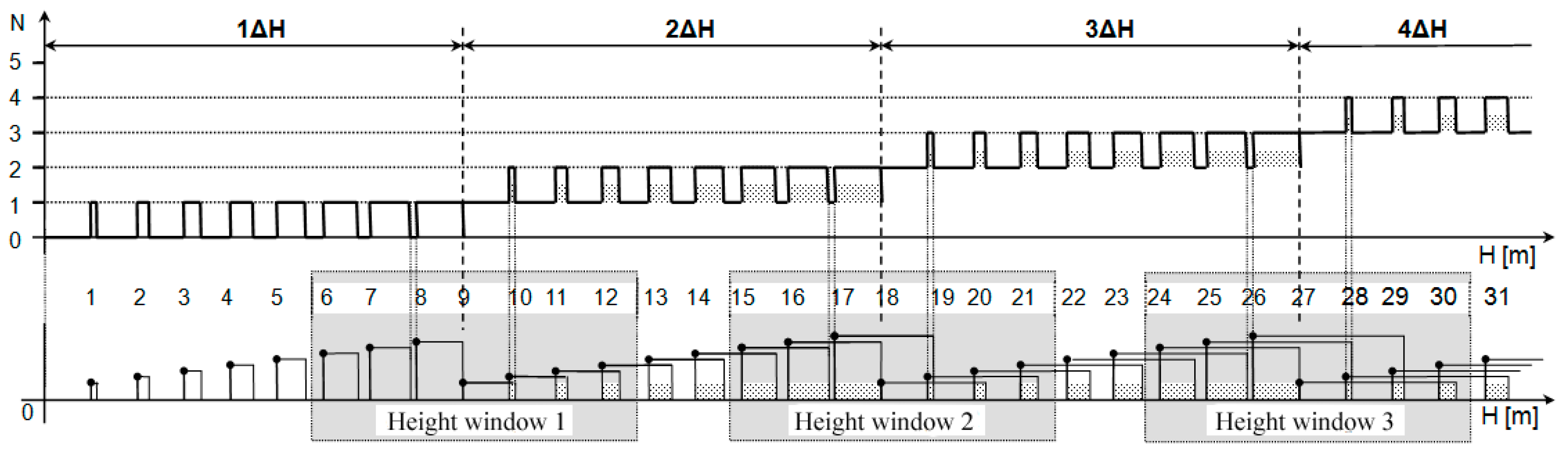
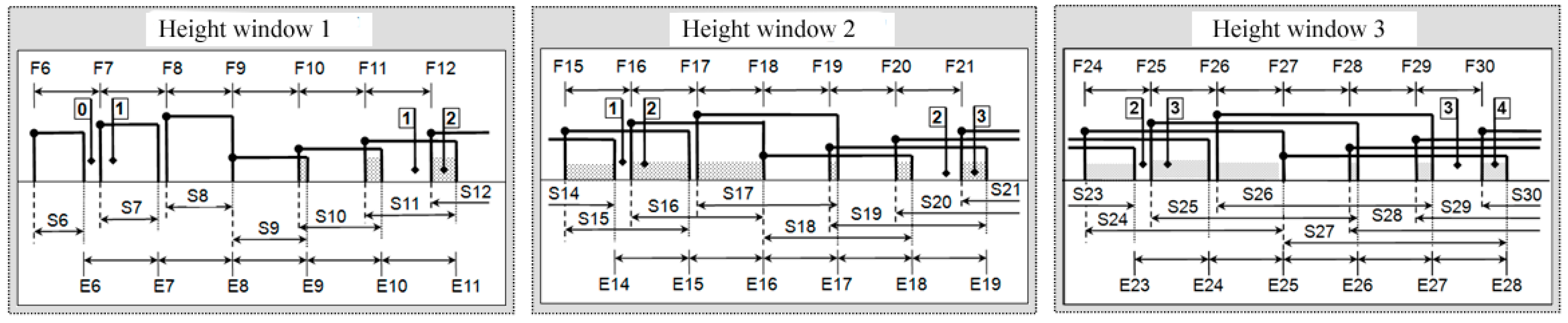
Then, the two heights behind the forming pulses make it possible to define the height range of the formation of individual pulses F, and from the two heights of the following dissolution pulses, Equation (4) is used to define the height range of dissolving pulses E:

$$F=H_{F2}- H_{F1}=\frac{{\lambda }_0}{4\left(1+\xi \right) },E=H_{E2}- H_{E1}=\frac{{\lambda }_0}{4\left(1-\xi \right) }.$$

(4)

A height range for the duration of the different unstable height pulse S is determined as the difference of height between the dissolution and formation of any height pulse:

$$S=H_E- H_F=\frac{{\lambda }_0}{4 }\left(2k-1\right)\frac{\xi }{1+{\xi }^2 }.$$

(5)

Equation (4) shows us that the height range of the gradual formation of the different unstable height pulses is constant and smaller than the value of λ₀/4 at any measured height. Thus, it is possible to state that F1 = F2 = F3 = …. At the same time, it can be seen that the height range of the dissolution of unstable pulses E is also constant but bigger than the value of λ₀/4 at any measured height. So, it is also possible to state that E1 = E2 = E3 = …. Equation (5) also indicates that the height range for the duration of the different unstable height pulses constantly grows with the increase of the consequence number of the pulse k, as a result of the increase of the value of measured altitude. So, it is possible to state that S1 < S2 < S3 < … [3,7].

Gradual increase of the height range for the duration of different unstable pulses together with the growing measured altitude cause more and more of those pulses at the same height to overlap mutually (Figure 1 and Figure 2) [13].

3. Simulation of Height Pulses Creation

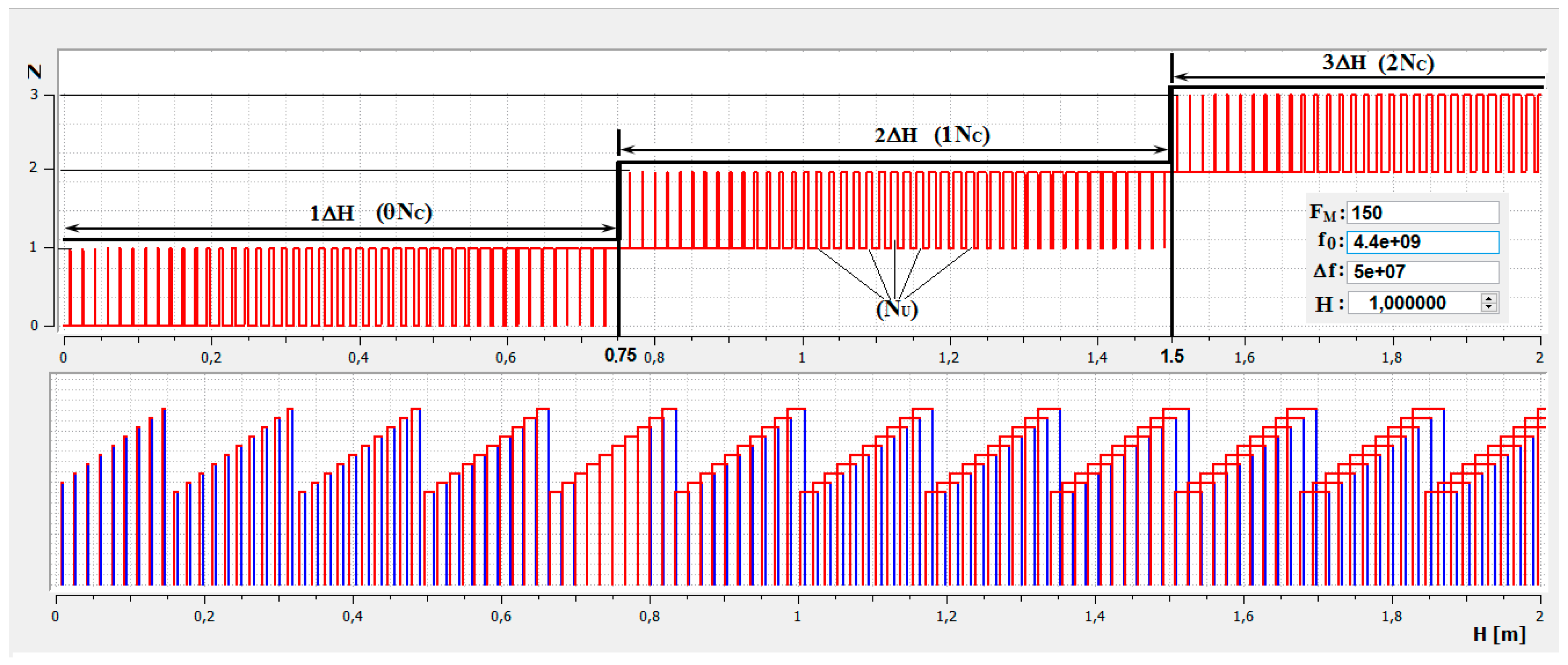
Based on the above-defined theory, the simulation program for making the stable and unstable height pulses of the radio altimeter has been created. The simulation results at the input parameters equal to the value of the current radio altimeters are shown in Figure 3. The simulation is realized in a height range from 0 m to 2 m, with a mean value of 1 m. In Figure 3, we can see that the first critical height value ends at the 0.75 m height level, and the second one ends at 1.5 m. Obviously, the methodic error of the radio altimeter (0.75 m) is the same as given by the radio altimeter manufacturers.

The upper part of Figure 3 represents the height dependence of the creation of numbers of stable (N_C) and unstable (N_U) height pulses. By the term “height pulses,” we express the correlation between the number of pulses in the frequency area and the measured altitude expressed in the unit of length. This can be partly compared to the correlation between the harmonic signal in the time domain and the number of periods in the frequency domain, as in Fourier transform. If we use a classical pulse generator, then changing the frequency setting will change the number of output pulses. If we record the generated pulses over time, there will be the time on the horizontal axis and amplitude on the vertical axis. However, if the number of pulses is evaluated in some non-standard but stable time, e.g., per modulation period, then we would plot the frequency on the horizontal axis and the number of pulses per modulation period on the vertical axis.

The radio altimeter is reminiscent of a quasi-pulse generator, which forms the number of pulses that correspond to the flight altitude. The peculiarity is that even with a fluent change in height, the number of pulses does not change fluently, but the formation and dissolution of the pulses are discrete, and their number creates a quantization (stairs) course when changing the altitude (Figure 3). This is due to the fact that the pulses do not occur in a separate low-frequency generator, but are formed from a differential frequency resulting from the mixing of the high frequency and frequency-modulated signals. Thus, when evaluating the number of radio altimeter pulses generated during the modulation period, where the altitude is the control parameter, then the height H is plotted on the horizontal axis, and the number of pulses N for the modulation period is plotted on the vertical axis.

The stable height pulses are those of which the number increases as the altitude increases gradually and discretely with the height range ΔH, that which creates the so-called quantization (stairs) course. In each height range (which is related to the altitude measurement accuracy), the number of these pulses is stable. The frequency value of these pulses is fixed to the altitude of the aircraft, which is expressed by the basic equation of a radio altimeter presented by Equation (12).

Unstable altitude pulses are those of which the number changes discreetly as the height increases, forming on every single stair ΔH a so-called comb course. In each height range ΔH, the formation and dissolution of the unstable pulse means that the total number of pulses within that range ΔH is changed by one pulse. The formation and dissolution of the unstable pulse occurs in a very small height range, so this situation is repeated in the range ΔH tens of times. The course of creation (formation and dissolution) of unstable pulses is the same in every height range ΔH (at each step). So, it is very interesting how many times the unstable pulse formation and dissolution will take place in the height range ΔH, as their number is related to the accuracy of the altitude measurement, which is the main topic of this manuscript.

In the 2 m height range, three critical heights are simulated, which correspond to the two ranges of the existence of the stable pulses 2Nc. There is no stable pulse in the first range (0Nc in 1ΔH in Figure 3). A larger number of unstable pulses are simulated in the same 2 m height range.

The bottom part of Figure 3 presents the height ranges of the duration of different pulses S. At the critical height of 1ΔH, the height ranges of the duration of the unstable height pulses are so small that they do not overlap, and an alternation of zero and the first unstable pulses (0–1) occur at the given critical height. At all the following critical heights, the height ranges of the duration of the unstable height pulses are so big that they mutually overlap. The number of permanently existing unstable pulses is determined by the consequence number of a stable height pulse. At least one unstable pulse exists at each section of the height within the range of 2ΔH. It means that one stable pulse exists at the height of alternation of the first and second unstable pulses (1–2) within the given range. Similarly, two unstable pulses exist permanently within the range of 3ΔH in each section of the height. It means that there are two stable pulses.

Closer analysis of this phenomenon can observe that the process of the formation and dissolution of the unstable height of pulses is not chaotic, but has regularity. The regularity of the formation and dissolution of the height pulses is related to the change in the measured height, but their number in the range of critical height corresponds to the technical parameters of the radio altimeter [11,12].

4. Number of Unstable Pulses in Range of Critical Height

It is obvious from Figure 1 and Figure 2, which present the height dependence of the formation of height pulses, as well as from Figure 3, which shows the results of the simulation of the stable and unstable height pulses, that the higher the number of unstable pulses is in the range of critical height, the smaller the precision of height measurement.

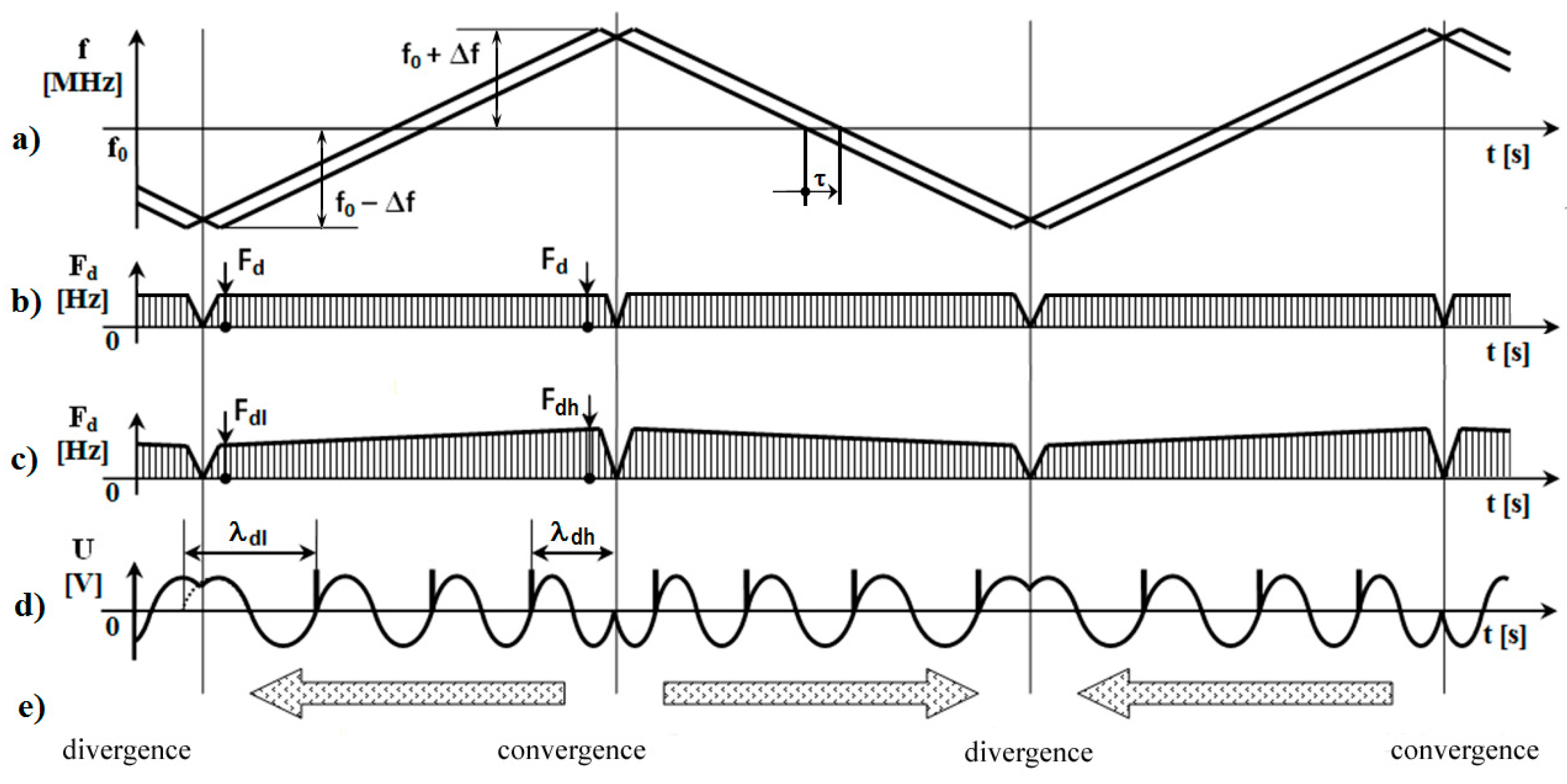
For the logical explanation of reasoning and determination of the number of unstable pulses in the range of critical height, it is necessary to move from the frequency area into the area of wavelengths. This thought is based on the generally known facts about the principle of the operation of FMCW radio altimeters presented in Figure 4.

Based on the principles that if the frequency modulation of the transmitted signal within the whole range of ±Δf is linear (Figure 4a), and that if the time delay of received signal during whole modulation period by value τ is also linear, then the immediate value of differential frequency is constant during whole time of the modulation period (Figure 4b). The areas of the changing of the direction of the frequency deviation in the areas of the maximum (f₀ + Δf)_max and minimum (f₀ − Δf)_min transmitted frequency are not considered.

However, the actual situation with the formation of the differential signal is different. The difference in frequency is not formed as a simple mathematical difference, but as interference of transmitted λ_T and received λ_R wavelengths. Then, the wavelength of the carrying signal is minimal λ_0min in the case of maximum transmitted frequency (f₀ + Δf)_max and, vice versa, the wavelength of carrying signal is maximal λ_0max at minimum transmitted frequency (f₀ − Δf)_min. With the equivalent time delay τ of the received signal within the whole modulation period but at the different wavelengths λ_0min and λ_0max, the value of difference frequency (interference) is not formed by the same way. At the wavelength of λ_0min, the interference is formed more often and the value of the higher difference frequency F_dh is higher and, vice versa, at the wavelength λ_0max, the interference is formed less frequently and the value of the lower difference frequency F_dl is smaller. Considering the presented phenomenon, the differential frequency is the same within the whole range of the modulation period (Figure 4c).

The above-presented theory is confirmed by the observation of realistic displays of the difference signal of a radio altimeter on an oscilloscope. In the higher frequency area f_0max and lower wavelength λ_0min, the higher differential frequency with the lower wavelength λ_dh will be formed with a higher number of the height pulses N. In the lower frequency area f_0min and the higher wavelength λ_0max, the lower difference frequency F_dl with the higher wavelength λ_dl will be formed with a lower number of the height pulses N (Figure 4d).

As a result of such unbalanced formation of differential frequency, and the fluent increase of the measured height, height pulses on the display of the oscilloscope will shift from the areas with the higher number of pulses into the area with the lower number of pulses. The presented shift of the periods of difference frequency and relevant height pulses is shown in Figure 4e.

Determination of the number of unstable pulses within the range of critical height ΔH is considered for a particular case of a radio altimeter with the carrier frequency of f₀ =4400 MHz, the modulation frequency of F_M = 150 Hz, and the frequency deviation of ±Δf = 25 MHz. In this case, we have f_0max = 4400 MHz + 25 MHz = 4425 MHz ⇒ λ_0min = 67.797 × 10⁻³ m, f₀ = 4400 MHz ⇒ λ₀ = 68.182 × 10⁻³ m, and f_0min = 4400 MHz − 25 MHz = 4375 MHz ⇒ λ_0max = 68.571 × 10⁻³ m.

Then, the difference of wavelengths can be defined λ_max − λ_min = 68.571 m − 67.797 m = 0.774 × 10⁻³ m.

The calculated value expresses the height range of the formation of an unstable height pulse. The half value of the number of the unstable height pulses within half a period of λ₀/2 of a carrier frequency f₀ presents the number of unstable pulses within the critical height ΔH. Thus, in the case of considered ratio altimeter, the number of unstable pulses is 44.

Figure 5 shows the results of the simulation of the formation of the number of unstable height pulses within the critical height ΔH for the particular type of a radio altimeter.

5. Number of Stable Pulses in Range of Critical Height

A recent method of increasing the accuracy of altitude measurement by the FMCW radio altimeters is based on the increase of frequency deviation with the simultaneous increase of the carrier signal frequency. However, the recent radio altimeters use the carrier frequency of 4.4 GHz with the frequency deviation of ±25 MHz (overall bandwidth of 50 MHz), and they can provide the measurement accuracy of ±0.75 m.

It is necessary to increase the carrier frequency with the increase of the frequency deviation due to the requirement for balanced frequency transmission characteristics of the high-frequency circuits, as well as active and passive elements of antennas. To increase the accuracy of the altitude measurement two-fold (to the value of ±0.375 m) by the same way, the value of the frequency deviation also should be increased two-fold (to the value of ±50 MHz that, in fact, corresponds to the overall bandwidth of 100 MHz), with the simultaneous increase of the carrier frequency approximately to 10 GHz.

Based on the above-analyzed theory, it is possible to avoid the problem of the necessity of using a higher carrier frequency of 10 GHz through the use of two parallel high-frequency channels at the original carrier frequency of 4.4 GHz. To create a performance signal, the frequency multipliers are commonly used in radio altimeters nowadays.

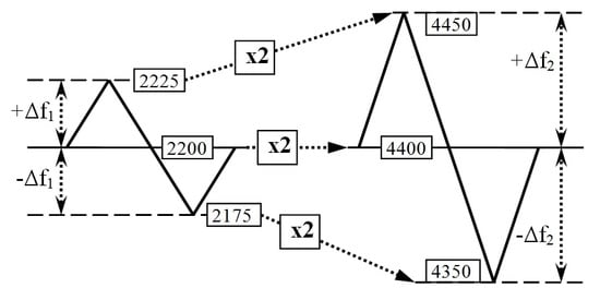
In such a way, a basic generator forms the frequency modulated signal with the center frequency of 2200 MHz and with the original frequency deviation ±Δf₁ = ±25 MHz. Then, the signal is divided by two frequency band-passes into two individual high-frequency channels. Each channel forms its own frequency deviation; the first channel has +Δf₁ from 2200 to 2225 MHz, and the second channel has −Δf₁ from 2175 to 2200 MHz.

Next, the frequency is independently multiplied two times into the value with the extreme frequency deviation of ±Δf₂ = ±50 MHz in each channel; the first channel has +Δf₂ from 4400 to 4450 MHz, and the second channel has −Δf₂ from 4350 to 4400 MHz (Figure 6). Each channel would only have a bandwidth that is commonly used, i.e., 50 MHz. At the same time, each channel is tuned in frequency to a different band, but the overall bandwidth is 100 MHz. The particular circuit connection of the radio altimeter with extreme bandwidth, which would comply with the above-presented condition, can be achieved by several solutions [14,15,16,17].

Based on the presented background, parameters of the critical height for a radio altimeter with extreme bandwidth have been analyzed with the help of simulation. The parameters of such a radio altimeter are as the following: the carrier frequency is 4400 MHz, the modulation frequency is 150 Hz, and the frequency deviation is 50 MHz, which in sum gives extreme bandwidth of 100 MHz (Figure 7).

From the viewpoint of altitude measurement precision, the results for the radio altimeter with extreme bandwidth are:

(a)

critical height has the value of 0.375 m;

(b)

methodological error of the radio altimeter is ±0.375 m;

(c)

simulated values are at the height of cca 5 m: 4.5 m, 4.875 m, and 5.25 m, respectively, for the bottom, mean, and upper values;

(d)

number of simulated unstable pulses subtracted within the range of the critical height is 22;

(e)

number of calculated unstable pulses within range of critical height is also 22.

Based on the theory presented in Section 4, the relation for the determination of the number of unstable pulses within the range of critical height has been derived as a part of the research:

$$N_U=\frac{f_0^2 - \Delta f^2}{2 f_0 \Delta f}.$$

(6)

From the above-presented results, it is possible to conclude that by using the double value of the total frequency deviation of 100 MHz at the carrier frequency of 4.4 GHz (a total frequency deviation of 50 MHz is recently used), it is possible to increase the accuracy of the height measurement two-fold. In this case, the critical height is 0.375 m, and it can be obtained by the formation of 22 unstable height pulses, but only when one stable pulse is formed. The unstable and stable pulses can be supported by the derivation of a basic equation of a radio altimeter from the height pulses formation [8].

The basic equation of a radio altimeter defines the relation between the value of the differential frequency and output information about the measured altitude, which is based on the basic parameters of a radio altimeter. Generally, known derivation comes out of the immediate difference of the frequencies of transmitted and received signals, proportionally to the time delay of the received signal, which depends on the measured altitude. A different method for a definition of a basic equation of a radio altimeter, based on critical height, has been derived during the research connected with the problem presented in the paper.

As it has been presented in this manuscript, a certain number of stable height pulses, shaped during the time of one modulation period T_M, corresponds to the measured altitude:

$$H=\frac{N}{T_M}.$$

(7)

The formation of only one stable height pulse during the time of one modulation period corresponds to the height change within the range of critical height:

$$\Delta H=\frac{1}{T_M}.$$

(8)

The following proportion can be obtained from Equations (7) and (8):

$$\frac{H}{\Delta H}=\frac{N/T_M}{1/T_M}.$$

(9)

Replacing the modulation period by the modulation frequency in Equation (9) we have:

$$\frac{H}{\Delta H}=\frac{N F_M}{F_M}.$$

(10)

The product of NF_M in Equation (10) presents the difference frequency, which is proportional to the altitude, so:

$$F_d=\frac{ F_M}{\Delta H}H.$$

(11)

Substitution of the critical height in Equation (11) from Equation (1) produces the basic equation of a radio altimeter presented in a completely different way from the generally known one, with the use of geometric similarity of triangles [18,19,20]:

$$F_d=\frac{8 \Delta f F_M}{c}H.$$

(12)

This fact proves all the above-presented theoretical consideration, which allows for an increase in the accuracy of the altitude measurement by a radio altimeter.

6. Software Application for Simulating the Unstable Pulses Creation

For the needs of the simulation and graphical display of the formation of the unstable pulses, a software application in Qt (C++) environment has been created. The algorithm is based on a theoretical analysis of the formation and dissolution of pulses when measuring altitude by a radio altimeter (Figure 8).

The individual values corresponding to the altitude of the pulse formation and dissolution depend on several parameters: the modulation frequency f_m = 70 MHz, carrier frequency f₀ = 444 MHz, and frequency deviation Δf = 8.5 MHz. One more parameter on the control panel is the choice of the mean value of the flight altitude H, around which the creation of the formation and dissolution of the unstable pulses is displayed. This is the altitude that is interesting for us from a certain point of view. The height range is limited to ±1 m because a wider height range would cause a graphical ambiguity. The last parameter displayed on the control panel represents the calculated number of stable pulses corresponding to the set height of the flight altitude H.

These parameters can be changed with regard to the specific or hypothetical type of radio altimeter and its technical parameters using the application control panel represented in Figure 9.

Figure 8 shows an example of the creation of unstable pulses for a set height of 4.6 m evaluated in the range of 3.6 m to 4.6 m. The parameters of the analyzed radio altimeter are shown in Figure 9.

The bottom part of the graph in Figure 8 shows the process of gradual formation and dissolution of a large number of individual height pulses, with a change in height H. The upper part of the graph presents the result of their mutual overlap by repeated formation and dissolution of one unstable pulse in the ΔH range. The number of repeated formations of a single unstable pulse in the ΔH range determines the accuracy of the altitude measurement. The resulting quantization (stairs) course of unstable pulses within the ΔH range shapes a number of stable pulses, which correspond to the measured altitude. The software application can be used to compare the height pulse creation and to simulate this process for different types of radio altimeters with various parameters.

7. Discussion and Conclusions

We have performed the analysis of the formation of the range of critical height of a radio altimeter methodological error when measuring the altitude. The analysis has been performed from the viewpoint of the determination of the number of unstable height pulses within the range of critical height. This manuscript focuses on the formation of unstable pulses within the range of critical height and explains the patterns between formation and dissolution of height pulses. As it is generally known, unstable pulses do not carry the information about measured altitude; they are not paid enough attention. Some works even consider the chaotic formation of the number of such pulses. Even though the unstable pulses do not determine measured altitude, and they have a critical influence on the precision of the height measurement.

Precise altitude measuring relates to the method of difference signal processing. The presented analysis supported by simulation has confirmed the applicability of the basic idea for the processing of the differential signal in the form of the creation of stable and unstable pulses.

The process of the determination of the number of unstable pulses within the range of critical height outlines a different view of the basic principle of a radio altimeter (shown in Figure 4c). An original and exact process of the determination of the number of unstable height pulses within the range of critical height for the recent radio altimeters is also presented. This method of calculation logically follows from Equation (6), which has successfully been verified in this manuscript for a different type of a radio altimeter.

The unique solution is based on the decrease of the value of the critical height by the decrease of the number of unstable pulses, which results in the doubled (extreme) increase of the frequency deviation at the original carrier frequency for the recent radio altimeters. In this way, the altitude measurement precision increases from the original value of ±0.75 m to the two-times lower value of ±0.375 m, without the need to increase the carrier frequency (two-fold). The correctness of this theory is highlighted by the new way of deriving the basic radio altimeter equation with the use of a critical height parameter. The results presented in the paper can be used for the design of new radio altimeters with the increased accuracy of the low altitude measurement.

References

- Nebylov, A.V. Aerospace Sensors; Momentum Press: New York, NY, USA, 2013; p. 348. ISBN 1-60650-059-7. [Google Scholar] [CrossRef]
- Kelemen, M.; Szabo, S. Pedagogical Research of Situational Management in Aviation Education and Forensic Investigation of Air Accidents: Knowledge of Aircraft Operation and Maintenance; Collegium Humanum: Warsaw, Poland, 2019; p. 144. ISBN 978-83-952951-1-9. [Google Scholar]
- Labun, J.; Adamčík, F.; Piľa, J.; Madarász, L. Effect of the measured pulses count on the methodical error of the air radio altimeter. Acta Polytech. Hung. 2010, 7, 41–49. [Google Scholar]
- Soták, M.; Labun, J. The new approach of evaluating differential signal of airborne FMCW radar-altimeter. Aerosp. Sci. Technol. 2012, 17, 1–6. [Google Scholar] [CrossRef]
- Stove, A.G. Linear FMCW radar techniques. IEE Proc. F (Radar Signal Process.) 1992, 139, 343–350. [Google Scholar] [CrossRef]
- Skolnik, M.I. Introduction to Radar Systems, 2nd ed.; McGraw Hill Book Company: Singapore, 1981; p. 581. ISBN 0-07-057909-1. [Google Scholar]
- Labun, J.; Soták, M.; Kurdel, P. Technical note innovative technique of using the radar altimeter for prediction of terrain collision threats. J. Am. Helicopter Soc. 2012, 57, 85–87. [Google Scholar] [CrossRef]
- Labun, J.; Krchňák, M.; Kurdel, P.; Češkovič, M.; Nekrasov, A.; Gamcová, M. Possibilities of increasing the low altitude measurement precision of airborne radio altimeters. Electronics 2018, 7, 191. [Google Scholar] [CrossRef]
- Taylor, J. Aircraft Operation of Radio Altimeters. In Proceedings of the 24th Meeting of Working Group F, Aeronautical Communications Panel (ACP), Paris, France, 17–21 March 2011. [Google Scholar]
- Alivizatos, E.G.; Petsios, M.N.; Uzunoglu, N.K. Architecture of a multistatic FMCW direction-finding radar. Aerosp. Sci. Technol. 2008, 12, 169–176. [Google Scholar] [CrossRef]
- Baskakov, A.I.; Komarov, A.A.; Mikhailov, M.S.; Ruban, A.V. Modeling of the methodical errors of high-precision aircraft radar altimeter operating above the seasurface at low altitudes. In Proceedings of the 2017 Progress in Electromagnetics Research Symposium—Spring (PIERS), St. Petersburg, Russia, 22–25 May 2017; pp. 3236–3240. [Google Scholar] [CrossRef]
- Singh, R.; Peterson, R.; Riaz, A.; Hood, C.; Bacchus, R.; Roberson, D. A method for evaluating coexistence of LTE and radar altimeters in the 4.2–4.4 GHz band. In Proceedings of the 2017 Wireless Telecommunications Symposium (WTS), Chicago, IL, USA, 26–28 April 2017; pp. 1–9. [Google Scholar]
- Liu, J.; Shen, C.; Wu, S.; Huang, W.; Li, C.; Zhu, Y.; Wang, L. Correction method of the manned spacecraft low altitude ranging based on γ ray. Aerosp. Sci. Technol. 2016, 50, 71–76. [Google Scholar] [CrossRef]
- Labun, J.; Grega, M.; Sopata, M.; Kmec, F. Aircraft Radio Altimeter for Small Heights with Frequency Modulation Design II. Patent 283439; Banská Bystrica, Slovak Republic, 20 June 2003. [Google Scholar]
- Grega, M.; Labun, J. Aircraft Radar Altimeter with Frequency Modulation Design. Patent 262626; Prague, Czechoslovak Republic, 16 August 1988. [Google Scholar]
- Kayton, M.; Fried, W.R. Avionics Navigation Systems; John Wieley & Sons: New York, NY, USA, 1997; p. 773. ISBN 0-471-54795-6. [Google Scholar]
- Nekrasov, A. Foundations for Innovative Application of Airborne Radars: Measuring the Water Surface Backscattering Signature and Wind; Springer: Dordrecht, The Netherlands, 2014; p. 116. ISBN 978-3-319-00620-8. [Google Scholar] [CrossRef]
- Fasano, G.; Accardo, D.; Tirri, A.E.; Moccia, A.; Lellis, E. Radio/electro-optical data fusion for non-cooperative UAS sense and avoid. Aerosp. Sci. Technol. 2015, 46, 436–450. [Google Scholar] [CrossRef]
- Metzger, J.; Meister, O.; Trommer, G.F.; Tumbrägel, F.; Taddiken, B. Adaptations of a comparison technique for terrain navigation. Aerosp. Sci. Technol. 2005, 9, 553–560. [Google Scholar] [CrossRef]
- Estrada, J.; Zurek, P.; Popović, Z. Harvesting of aircraft radar altimeter side lobes for low-power sensors. In Proceedings of the 2018 International Applied Computational Electromagnetics Society Symposium (ACES 2018), Denver, CO, USA, 24–29 March 2018; pp. 1–2. [Google Scholar] [CrossRef]
© 2019 by the authors. Licensee MDPI, Basel, Switzerland. This article is an open access article distributed under the terms and conditions of the Creative Commons Attribution (CC BY) license (http://creativecommons.org/licenses/by/4.0/).