Entropy-Based Low-Rank Approximation for Contrast Dielectric Target Detection with Through Wall Imaging System


Abstract
1. Introduction
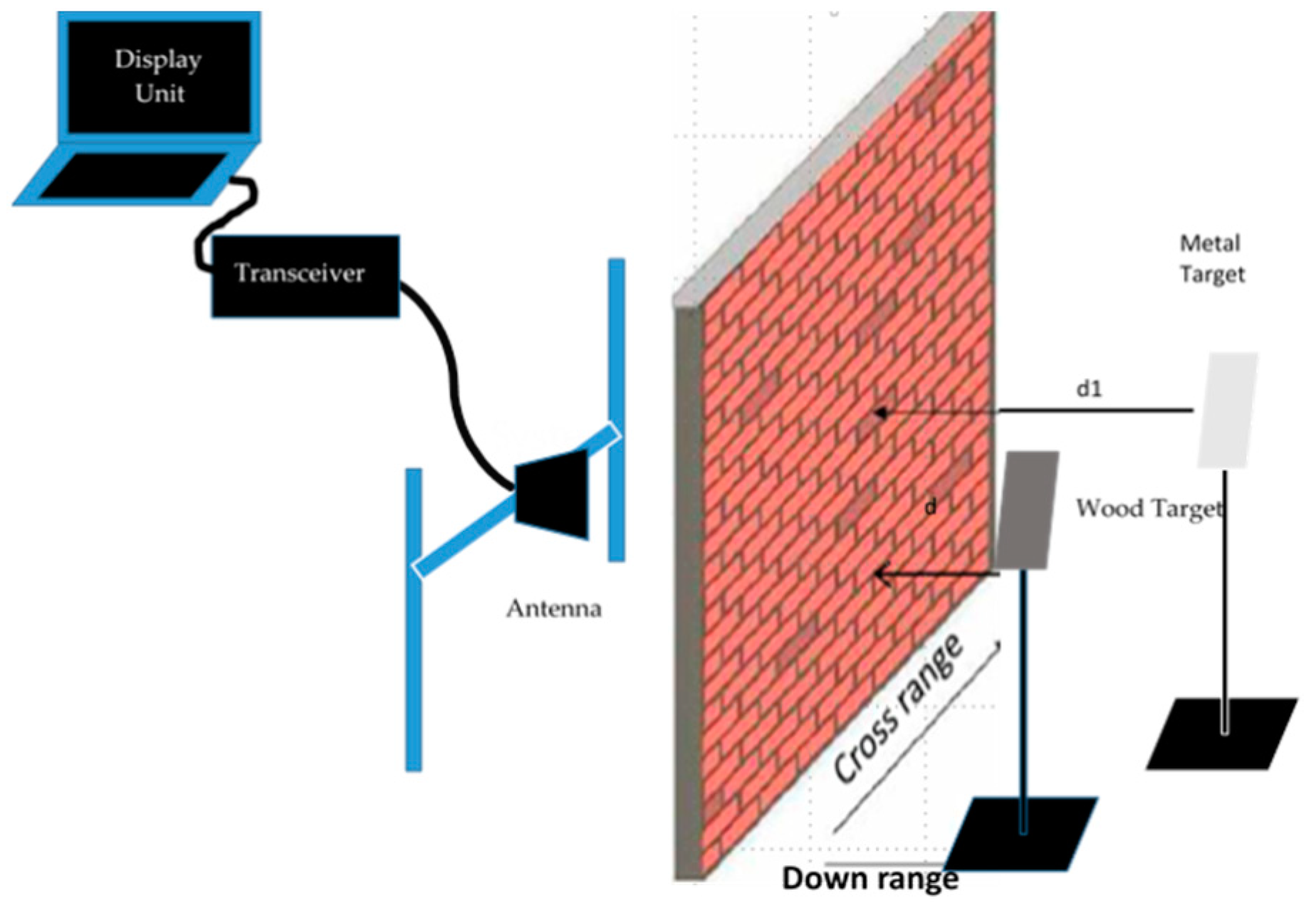
2. TWI Data Collection and Beamforming
2.1. Data Collection
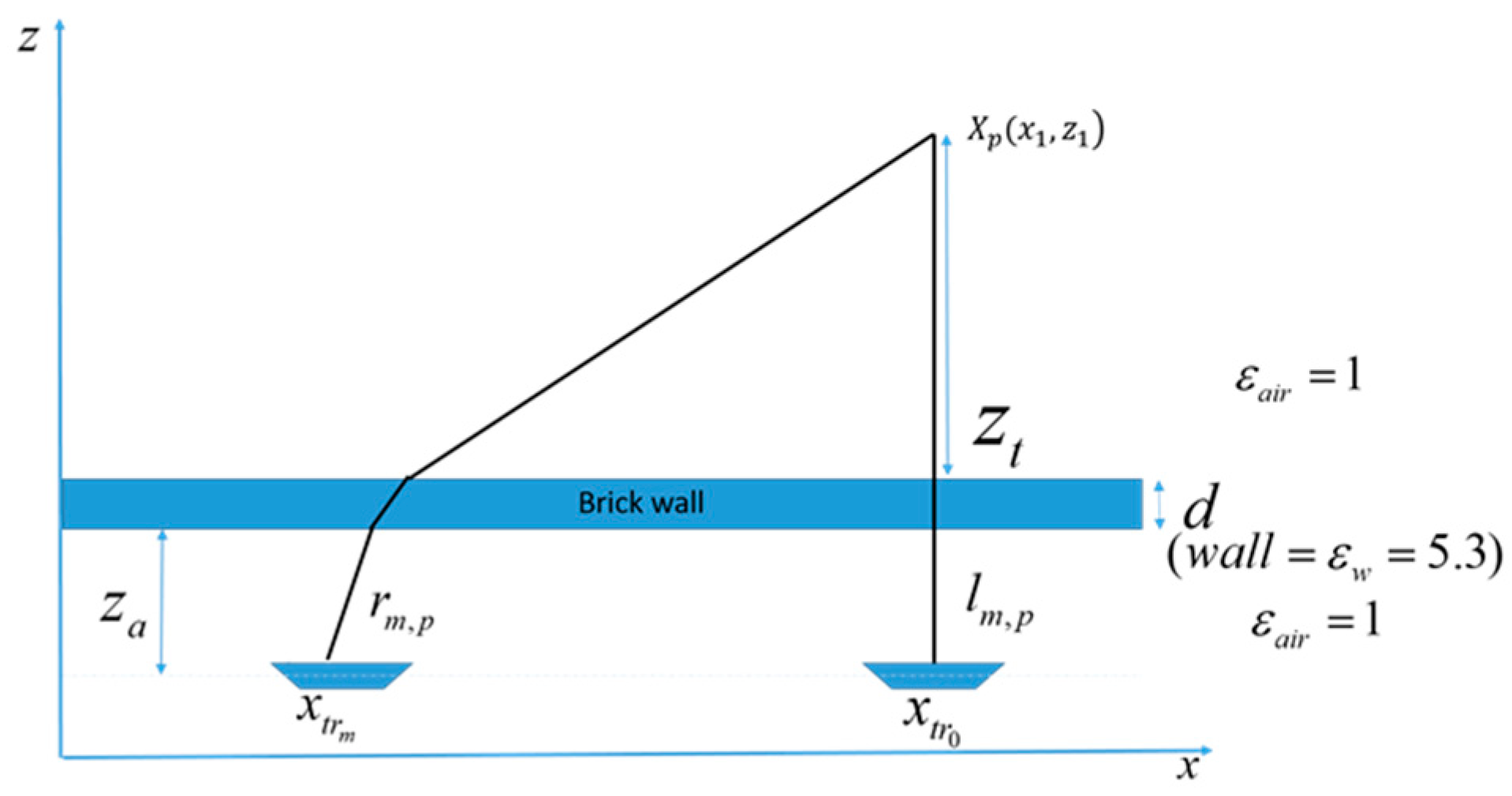
2.2. Beamforming
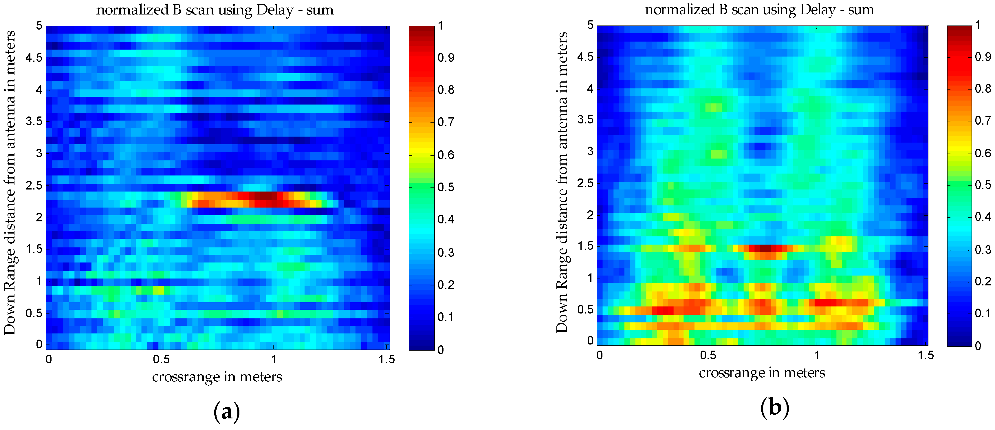
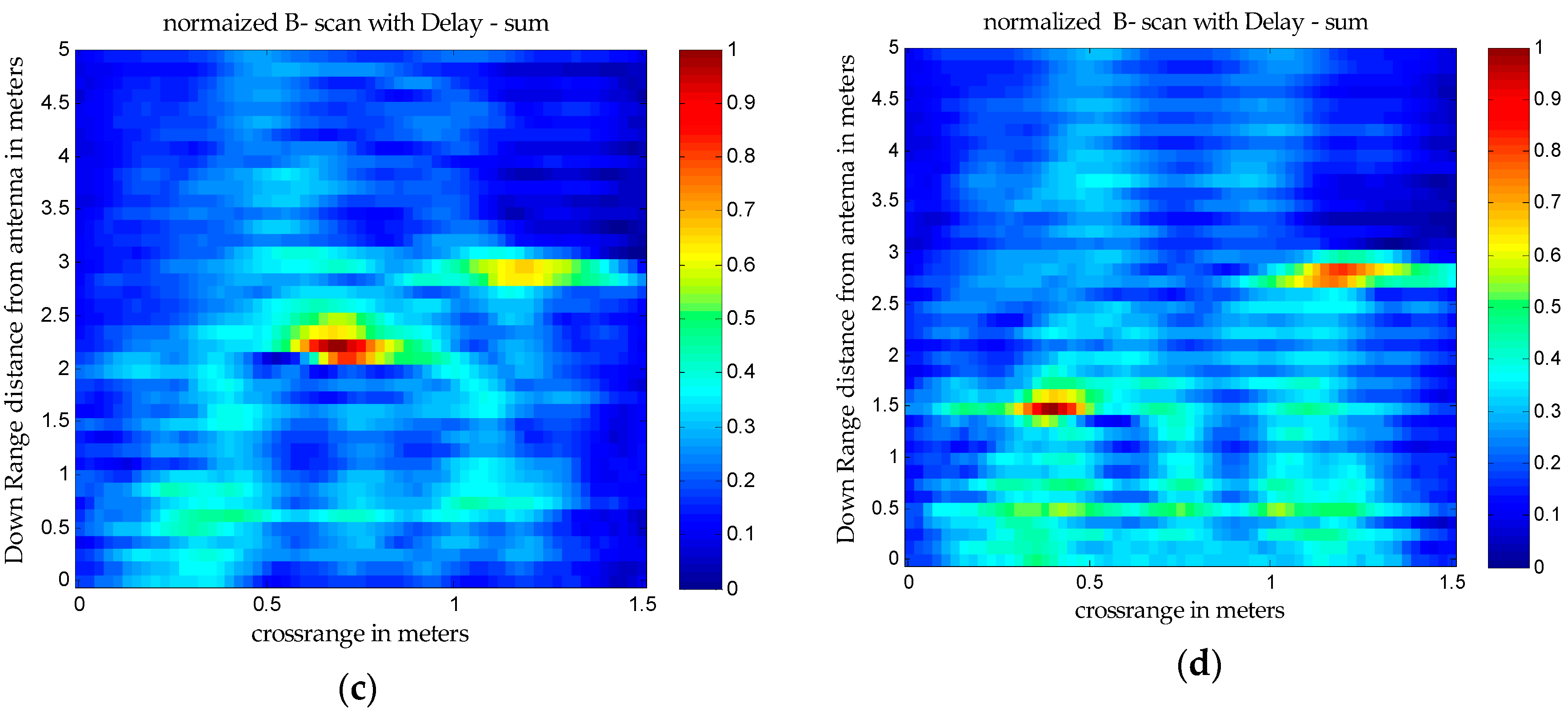
3. Clutter Reduction Techniques
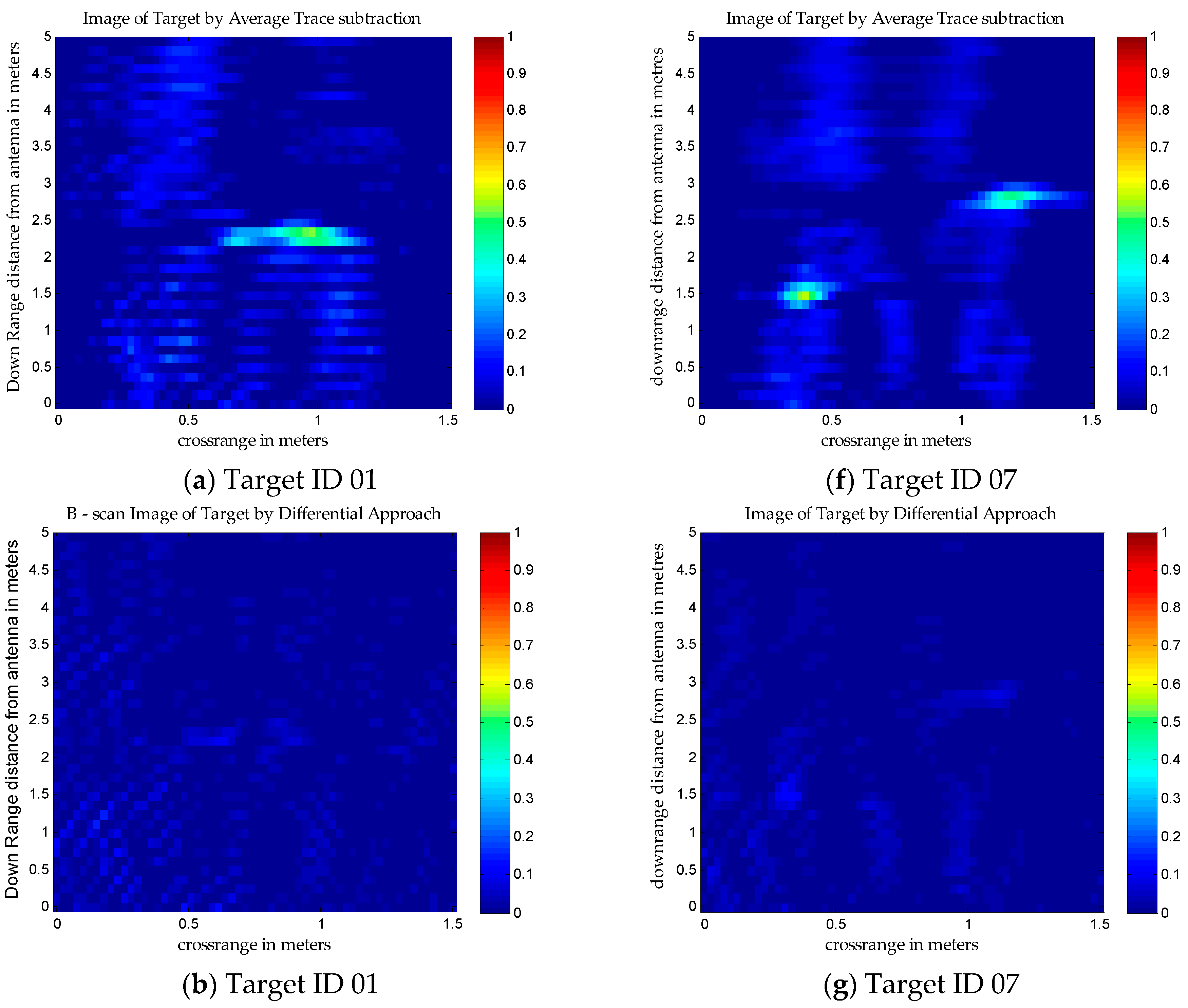
3.1. Average Trace Subtraction
3.2. Differential Approach
3.3. Subspace Projection Approach
3.3.1. Singular Value Decomposition (SVD)
3.3.2. Independent Component Analysis (ICA)
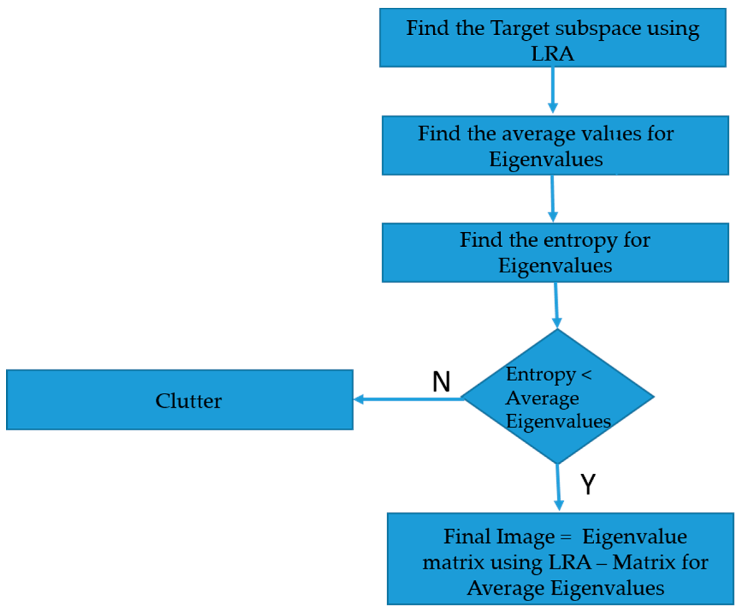
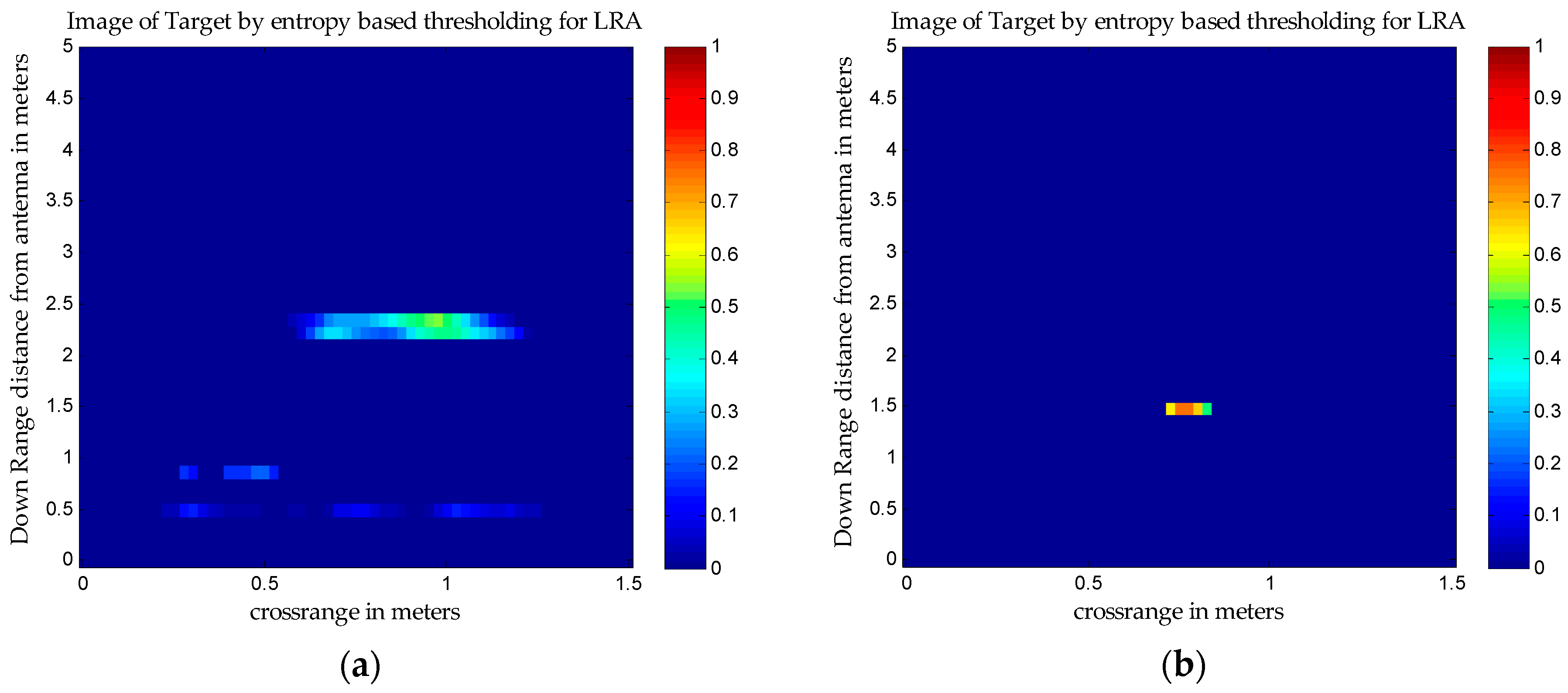
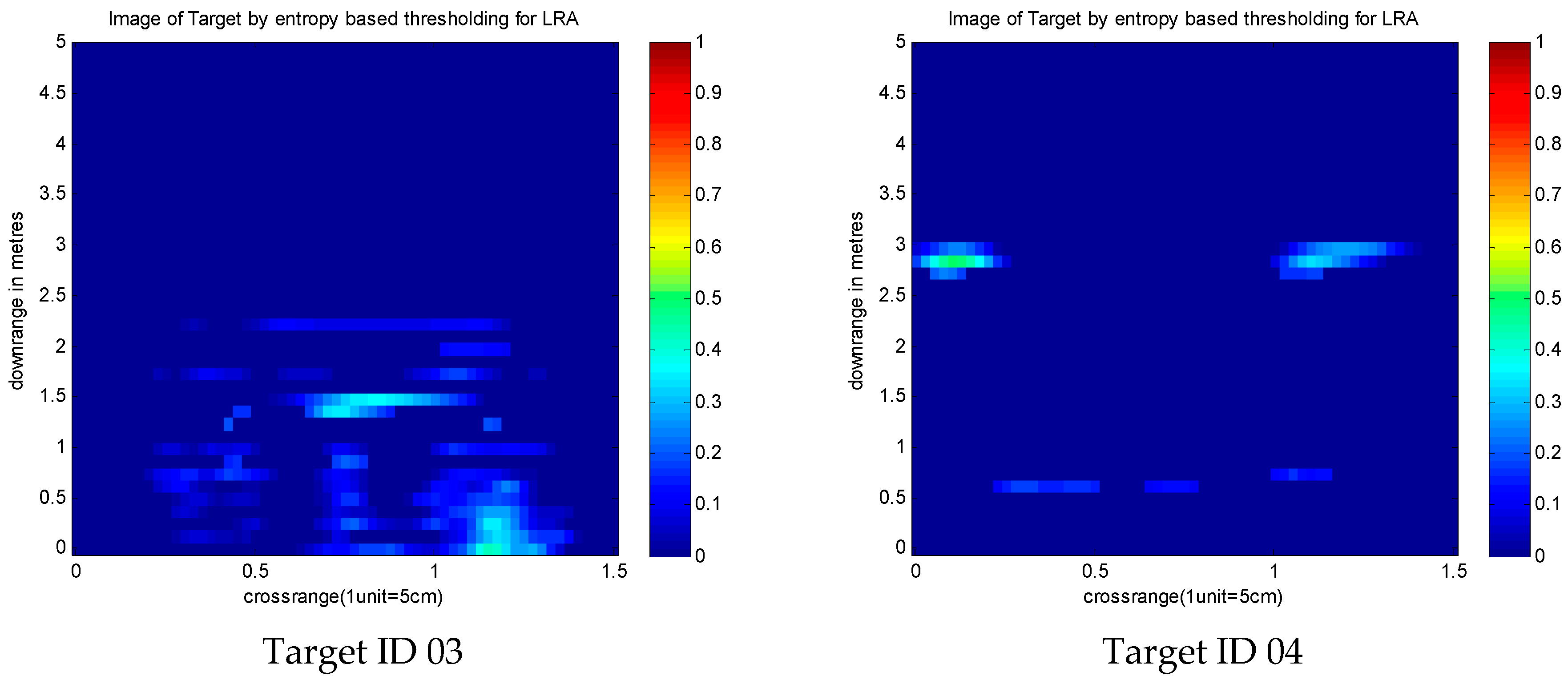
3.4. Entropy-based Time Gating
- MSE—Mean square error
- O.I.—Original normalized image
- F.I.—Final image
- V.P.—Number of vertical scanning points
- H.P.—Number of horizontal scanning points
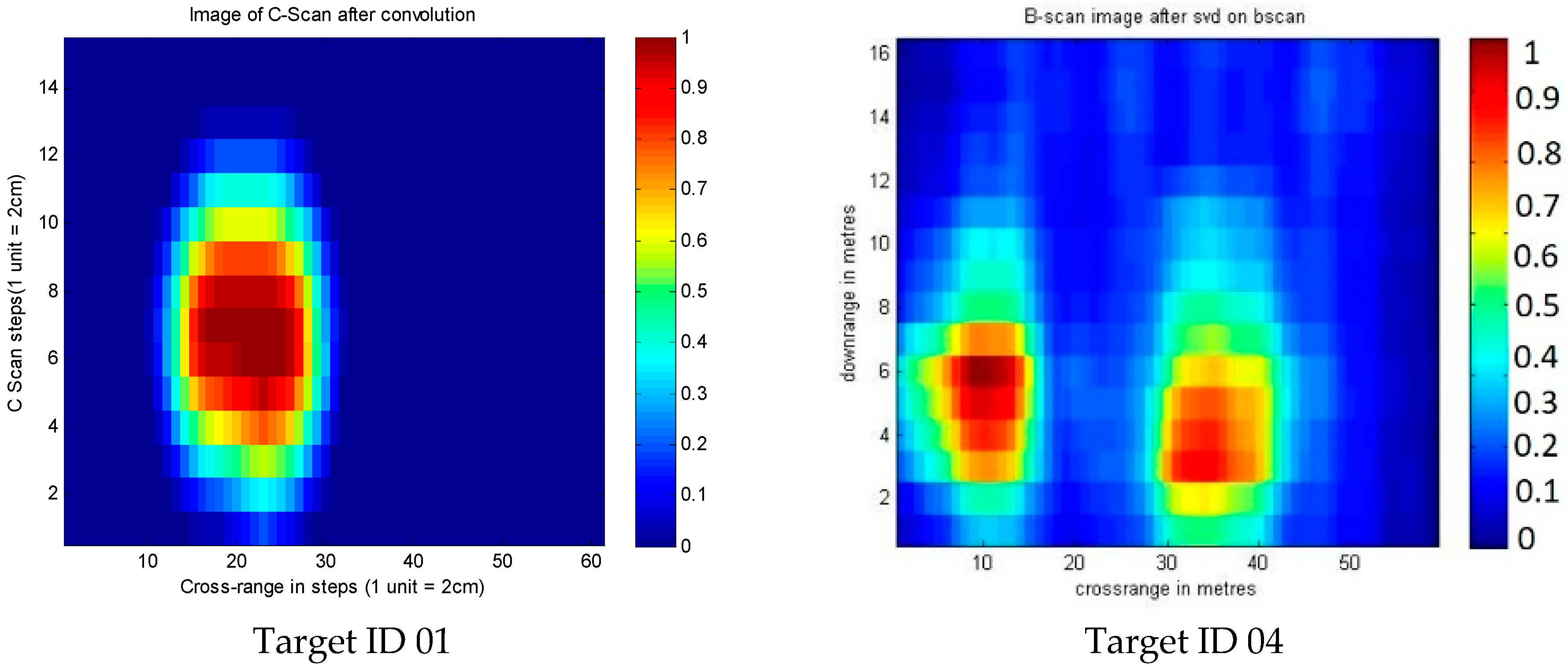
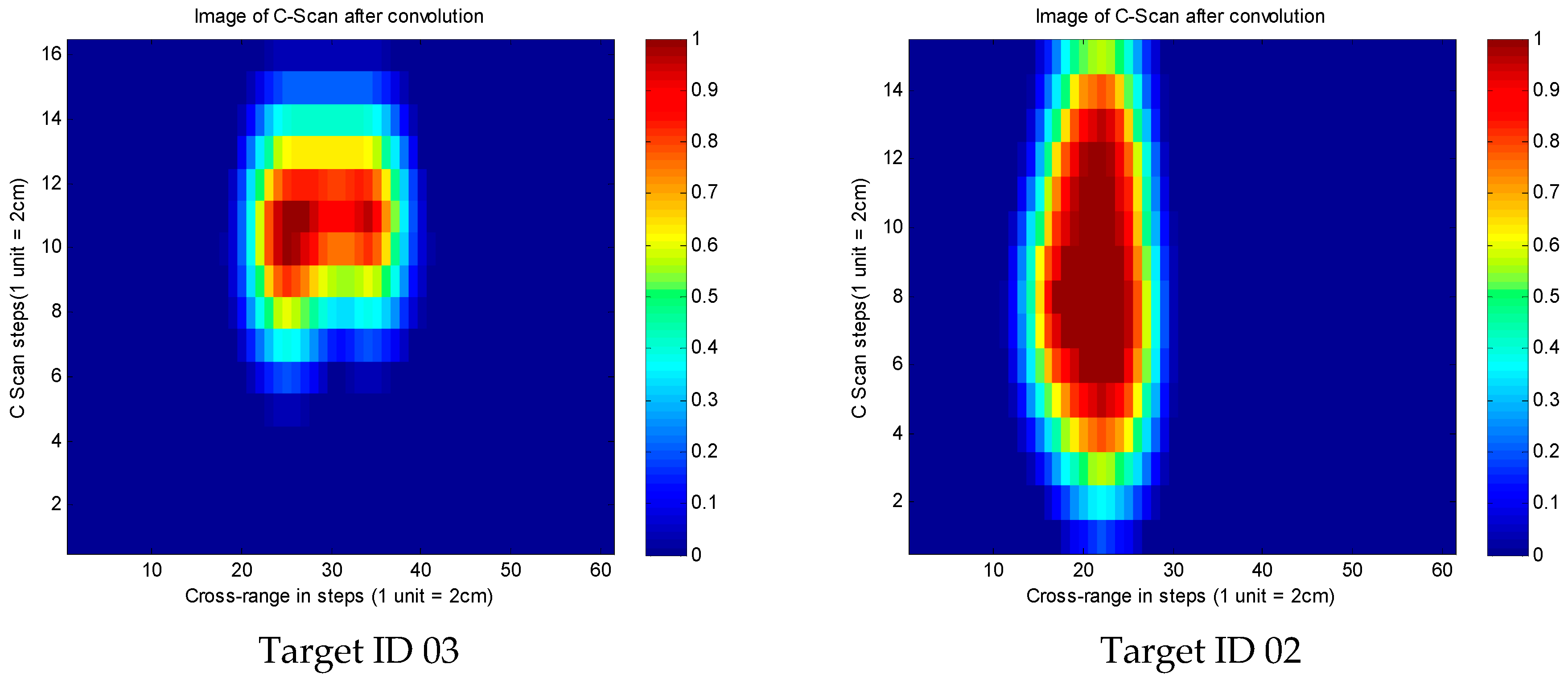
4. A Proposed Novel Method for Contrast Imaging
5. Conclusions
Author Contributions
Funding
Conflicts of Interest
Appendix A

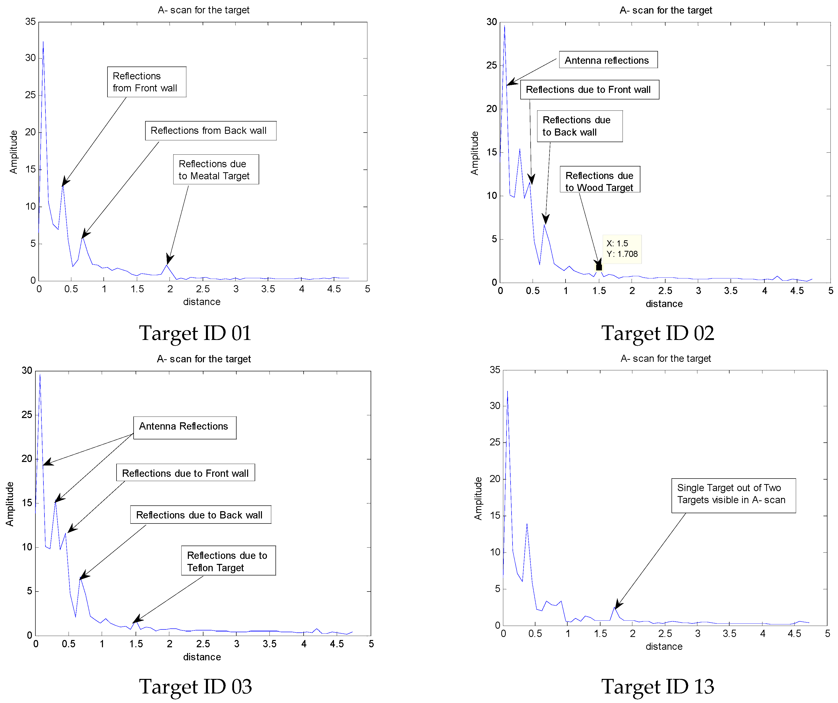
| Target ID | Number of Targets | Target Type | The Distance of the Targets from the Antenna Mouth | Target Size/Thickness |
|---|---|---|---|---|
| 01 | 01 | Metal | 2.3 m | 17.5 cm × 14.5 cm/1 cm |
| 02 | 01 | Wood | 1.5 m | Thick wood: 50 cm × 30 cm/2 cm Thin wood: 30 cm × 30 cm/1 cm |
| 03 | 01 | Teflon | 1.5 m | 50 cm × 40 cm/1 cm |
| 04 | 02 | Metal-Metal | 3 m | 17.5 cm × 14.5 cm/1 cm |
| 05 | 02 | Metal-Metal | 2.3 m and 3 m | 17.5 cm × 14.5 cm/1 cm |
| 06 | 02 | Metal-Wood | 1.73 m | 17.5 cm × 14.5 cm/1 cm, Thick wood: 50 cm × 30 cm/2 cm |
| 07 | 02 | Metal-Wood | 2.3 m and 1.5 m | 17.5 cm × 14.5 cm/1 cm, Thick wood: 50 cm × 30 cm/2 cm |
| 08 | 02 | Metal-Teflon | 2.3 m | 17.5 cm × 14.5 cm/1 cm, 50 cm × 40 cm/1 cm |
| 09 | 02 | Metal-Teflon | 2.3 m and 1 m | 17.5 cm × 14.5 cm/1 cm, 50 cm × 40 cm/1 cm |
| 10 | 02 | Wood (thick)–Wood (thin) | 1.73 m | Thick wood: 50 cm × 30 cm/2 cm Thin wood: 30 cm × 30 cm/ 1 cm |
| 11 | 02 | Wood (thick)–Wood (thin) | 3.5 m and 2.5 m | Thick wood: 50 cm × 30 cm/2 cm Thin wood: 30 cm × 30 cm/1 cm |
| 12 | 03 | Metal Wood (Thick)-Wood (thin) | 1.5 m | 17.5 cm × 14.5 cm/ 1 cm, Thick wood: 50 cm × 30 cm/2 cm Thin wood: 30 cm × 30 cm/ 1 cm |
| 13 | 03 | Metal-Wood (Thick)-Wood (thin) | 3.5 m, 2.5 m, 1.5 m | 17.5 cm × 14.5 cm/ 1 cm, Thick wood: 50 cm × 30 cm/2 cm Thin wood: 30 cm × 30 cm/1 cm |


References
- Verma, P.K.; Gaikwad, A.N.; Singh, D.; Nigam, M.J. Analysis of Clutter Reduction Techniques for through Wall Imaging in UWB Range. Prog. Electromagn. Res. 2009, 17, 29–48. [Google Scholar] [CrossRef]
- Potin, D.; Duflos, E.; Vanheeghe, P. Landmines Ground-Penetrating Radar Signal Enhancement by Digital Filtering. IEEE Trans. Geosci. Remote Sens. 2006, 44, 2393–2406. [Google Scholar] [CrossRef]
- van der Merwe, A.; Gupta, I.J. A novel signal processing technique for clutter reduction in GPR measurements of small, shallow land mines. IEEE Trans. Geosci. Remote Sens. 2000, 38, 2627–2637. [Google Scholar]
- Daniels, D.J. A review of landmine detection using GPR. In Proceedings of the 2008 European Radar Conference, Amsterdam, Netherlands, 30–31 October 2008; pp. 280–283. [Google Scholar]
- van Kempen, L.; Sahli, H. Signal processing techniques for clutter parameters estimation and clutter removal in GPR data for landmine detection. In Proceedings of the 11th IEEE Signal Processing Workshop on Statistical Signal Processing (Cat. No.01TH8563), Singapore, 8 August 2001; pp. 158–161. [Google Scholar]
- Zoubir, A.M.; Chant, I.J.; Brown, C.L.; Barkat, B.; Abeynayake, C. Signal processing techniques for landmine detection using impulse ground penetrating radar. IEEE Sens. J. 2002, 2, 41–51. [Google Scholar] [CrossRef]
- Gaikwad, A.N.; Singh, D.; Nigam, M.J. Application of clutter reduction techniques for detection of metallic and low dielectric target behind the brick wall by stepped frequency continuous wave radar in ultra-wideband range. IET Radar Sonar Navig. 2011, 5, 416–425. [Google Scholar] [CrossRef]
- Tivive, F.H.C.; Bouzerdoum, A.; Amin, M.G. A Subspace Projection Approach for Wall Clutter Mitigation in Through-the-Wall Radar Imaging. IEEE Trans. Geosci. Remote Sens. 2015, 53, 2108–2122. [Google Scholar] [CrossRef]
- Tebchrany, E.; Sagnard, F.; Baltazart, V.; Tarel, J.; Dérobert, X. Assessment of statistical-based clutter reduction techniques on ground-coupled GPR data for the detection of buried objects in soils. In Proceedings of the 15th International Conference on Ground Penetrating Radar, Brussels, Belgium, 30 June–4 July 2014; pp. 604–609. [Google Scholar]
- Tivive, F.H.C.; Bouzerdoum, A.; Amin, M.G. An SVD-based approach for mitigating wall reflections in through-the-wall radar imaging. In Proceedings of the 2011 IEEE RadarCon (RADAR), Kansas City, MO, USA, 23–27 May 2011; pp. 519–524. [Google Scholar]
- Tivive, F.H.C.; Amin, M.G.; Bouzerdoum, A. Wall clutter mitigation based on eigen-analysis in through-the-wall radar imaging. In Proceedings of the 2011 17th International Conference on Digital Signal Processing (DSP), Corfu, Greece, 6–8 July 2011; pp. 1–8. [Google Scholar]
- Chen, Y.; Zhou, Y.; Chen, W.; Zu, S.; Huang, W.; Zhang, D. Empirical Low-Rank Approximation for Seismic Noise Attenuation. IEEE Trans. Geosci. Remote Sens. 2017, 55, 4696–4711. [Google Scholar] [CrossRef]
- Mohsin Riaz, M.; Ghafoor, A. Through-Wall Image Enhancement Based on Singular Value Decomposition. Available online: https://www.hindawi.com/journals/ijap/2012/961829/ (accessed on 29 May 2018).
- Zhang, Y.; Xia, T. In-Wall Clutter Suppression Based on Low-Rank and Sparse Representation for Through-the-Wall Radar. IEEE Geosci. Remote Sens. Lett. 2016, 13, 671–675. [Google Scholar] [CrossRef]
- Wang, G.; Amin, M. A new approach for target location of through the wall radar imaging in the presence of wall ambiguities. In Proceedings of the Fourth IEEE International Symposium on Signal Processing and Information Technology, Rome, Italy, 18–21 December 2004; pp. 183–186. [Google Scholar]
- Boje, E. Fast discrete Fourier transform with exponentially spaced points. IEEE Trans. Signal Process. 1995, 43, 3033–3035. [Google Scholar] [CrossRef]
- Nicolaescu, I.; Genderen, P. van Procedures to improve the performances of a Sfcw radar used for landmine detection. In Proceedings of the 2008 Microwaves, Radar and Remote Sensing Symposium, Kiev, Ukraine, 22–24 September 2008; pp. 250–255. [Google Scholar]
- Mikhnev, V.A.; Vainikainen, P. Single-reference near-field calibration procedure for step-frequency ground penetrating radar. IEEE Trans. Geosci. Remote Sens. 2003, 41, 75–80. [Google Scholar] [CrossRef]
- Ahmad, F.; Amin, M.G.; Kassam, S.A. A beamforming approach to stepped-frequency synthetic aperture through-the-wall radar imaging. In Proceedings of the 1st IEEE International Workshop on Computational Advances in Multi-Sensor Adaptive Processing, Puerto Vallarta, Mexico, 13–15 December 2005; pp. 24–27. [Google Scholar]
- Kaushal, S.; Kumar, B.; Singh, D. An autofocusing method for imaging the targets for TWI radar systems with correction of thickness and dielectric constant of wall. Int. J. Microw. Wirel. Technol. 2019, 11, 15–21. [Google Scholar] [CrossRef]
- Yao, Q.; Qifu, W. Kirchoff Migration Algorithm for Ground Penetrating Radar Data. In Proceedings of the 2012 International Conference on Computer Science and Electronics Engineering, Hangzhou, China, 23–25 March 2012; Volume 2, pp. 396–398. [Google Scholar]
- Yektakhah, B.; Dehmollaian, M. A Method for Cancellation of Clutter Due to an Object in Transceiver Side of a Wall for Through-Wall Sensing Applications. IEEE Geosci. Remote Sens. Lett. 2012, 9, 559–563. [Google Scholar] [CrossRef]
- Kumar, B.; Upadhyay, R.; Singh, D. Development of an Adaptive Approach for Identification of Targets (Match Box, Pocket Diary and Cigarette Box) under the Cloth with MMW Imaging System. Prog. Electromagn. Res. 2017, 77, 37–55. [Google Scholar] [CrossRef]
- Kumar, B.; Sharma, P.; Singh, D. Development of an efficient approach for MMW imaging system to identify concealed targets inside the book. Microw. Opt. Technol. Lett. 2017, 59, 2982–2990. [Google Scholar] [CrossRef]
- Solimene, R.; Cuccaro, A. Front Wall Clutter Rejection Methods in TWI. IEEE Geosci. Remote Sens. Lett. 2014, 11, 1158–1162. [Google Scholar] [CrossRef]
- Yoon, Y.S.; Amin, M.G. Spatial Filtering for Wall-Clutter Mitigation in Through-the-Wall Radar Imaging. IEEE Trans. Geosci. Remote Sens. 2009, 47, 3192–3208. [Google Scholar] [CrossRef]
- Dehmollaian, M.; Thiel, M.; Sarabandi, K. Through-the-Wall Imaging Using Differential SAR. IEEE Trans. Geosci. Remote Sens. 2009, 47, 1289–1296. [Google Scholar] [CrossRef]
- Hyvarinen, A. Fast and robust fixed-point algorithms for independent component analysis. IEEE Trans. Neural Netw. 1999, 10, 626–634. [Google Scholar] [CrossRef] [PubMed]
- Stickley, G.F.; Noon, D.A.; Cherniakov, M.; Longstaff, I.D. Gated stepped-frequency ground penetrating radar. J. Appl. Geophys. 2000, 43, 259–269. [Google Scholar] [CrossRef]


| Sr. No. | Parameters | Value |
|---|---|---|
| 01 | Radar type | SFCW |
| 02 | Frequency range | 1 GHz–3 GHz |
| 03 | Transmitted power | 3 dBm |
| 04 | Number of frequency points | 201 |
| 05 | Bandwidth | 2 GHz |
| 06 | Cross-range resolution | 15 cm |
| 07 | Down-range resolution | 7.5 cm |
| 08 | Polarization | VV |
| 09 | Antenna type | Horn |
| 10 | Gain of Antenna | 20 dB |
| 11 | Beam-width | 15.92° and 17.02° |
| Sr. No. | Clutter Reduction Method | PSNR in dB |
|---|---|---|
| 1. | Average trace subtraction | 10.7504 |
| 2. | Singular value decomposition | 7.6220 |
| 3. | Differential approach | 10.1494 |
| 4. | Independent component analysis | 12.6255 |
| Sr. No. | Clutter Reduction Method | PSNR in dB |
|---|---|---|
| 1. | Average trace subtraction | 9.9608 |
| 2. | Singular value decomposition | 9.8052 |
| 3. | Differential approach | 9.3390 |
| 4. | Independent component analysis | 12.8549 |
© 2019 by the authors. Licensee MDPI, Basel, Switzerland. This article is an open access article distributed under the terms and conditions of the Creative Commons Attribution (CC BY) license (http://creativecommons.org/licenses/by/4.0/).
Share and Cite
Bivalkar, M.; Singh, D.; Kobayashi, H. Entropy-Based Low-Rank Approximation for Contrast Dielectric Target Detection with Through Wall Imaging System. Electronics 2019, 8, 634. https://doi.org/10.3390/electronics8060634
Bivalkar M, Singh D, Kobayashi H. Entropy-Based Low-Rank Approximation for Contrast Dielectric Target Detection with Through Wall Imaging System. Electronics. 2019; 8(6):634. https://doi.org/10.3390/electronics8060634
Chicago/Turabian StyleBivalkar, Mandar, Dharmendra Singh, and Hirokazu Kobayashi. 2019. "Entropy-Based Low-Rank Approximation for Contrast Dielectric Target Detection with Through Wall Imaging System" Electronics 8, no. 6: 634. https://doi.org/10.3390/electronics8060634
APA StyleBivalkar, M., Singh, D., & Kobayashi, H. (2019). Entropy-Based Low-Rank Approximation for Contrast Dielectric Target Detection with Through Wall Imaging System. Electronics, 8(6), 634. https://doi.org/10.3390/electronics8060634