Abstract
In inverse synthetic aperture radar (ISAR) imaging, time-frequency analysis is the basic method for processing echo signals, which are reflected by the results of time-frequency analysis as each component changes over time. In the time-frequency map, a target’s rigid body components will appear as a series of single-frequency signals in the low-frequency region, and the micro-Doppler components generated by the target’s moving parts will be distributed in the high-frequency region with obvious frequency modulation. Among various time-frequency analysis methods, S-transform is especially suitable for analyzing these radar echo signals with micro-Doppler (m-D) components because of its multiresolution characteristics. In this paper, S-transform and the corresponding synchrosqueezing method are used to analyze the ISAR echo signal and perform imaging. Synchrosqueezing is a post-processing method for the time-frequency analysis result, which could retain most merits of S-transform while significantly improving the readability of the S-transformation result. The results of various simulations and actual data will show that S-transform is highly matched with the echo signal for ISAR imaging: the better frequency-domain resolution at low frequencies can concentrate the energy of the rigid body components in the low-frequency region, and better time resolution at high frequencies can better describe the transformation of the m-D component over time. The combination with synchrosqueezing also significantly improves the effect of time-frequency analysis and final imaging, and alleviates the shortcomings of the original S-transform. These results will be able to play a role in subsequent work like feature extraction and parameter estimation.
1. Introduction
In inverse synthetic aperture radar (ISAR) imaging, to obtain the final image, two steps of Fourier transform are necessary for the original echo signal. Through the Fourier transform, the periodic characteristics of the time domain signal are found and reflected in the frequency domain. With the periodic characteristics in different dimensions combined with the appropriate resolution, the shape information of the target can be obtained [1].
In these radar echo signals, the rigid body part of the target and the moving part will produce two types of component. The latter will be referred to as the micro-Doppler (m-D) component with frequency modulation, which may generate from rotation of propellers or rotor wings on plane, surface vibration caused by engine, and swinging arms when human walk may cause the m-D effect [2,3].
The m-D component usually interferes with the final imaging result, but on the other hand, it can also be used for feature extraction and parameter estimation of the target, which is useful information in subsequent work [4]. However, in the face of such components, the simple Fourier transform cannot analyze the transformation of their frequency domain characteristics with time. For this reason, time-frequency analysis, which was born to characterize the transformation of signals in the frequency domain over time, has been applied to this field and has become one of the most basic analysis methods for m-D components [1,5,6].
Among many time-frequency analysis methods, S-transform (ST) is especially suitable for analyzing radar echo signals for imaging [7]. The multiresolution characteristics of S-transform are consistent with ISAR’s signal type. Its high frequency domain resolution in the low-frequency region can achieve accurate imaging of the target’s rigid body component, while the time domain resolution advantage of the high frequency region can effectively provide target micro-Doppler information.
S-transform can be further combined with the synchrosqueezing transform (SST) method to further improve the concentration of the time-frequency analysis results [8]. The algorithm performs synchronous squeezing of the time-frequency map in the frequency domain, which improves the concentration while inverse transformation, in a strict mathematical sense, can be ensured. Therefore, SST can not only do analysis from the time domain to the time-frequency domain, but can also hold the synthesis from the time-frequency domain to the time domain. Recently, by adopting the second-order operator, second-order synchrosqueezing (SST2) has been able to analyze a strong frequency-modulated signal [9,10,11].
In this paper, S-transform and second-order synchrosqueezing methods are applied to ISAR imaging. Both the simulation and the actual signal will have the benefit of the multiresolution characteristics of the S-transform when analyzing radar echo signals containing micro-Doppler components. Synchrosqueezing, on the basis of retaining these characteristics, greatly improves the readability of time-frequency analysis results, which brings more favorable conditions for subsequent work. The arrangement of this paper is as follows. A brief introduction of ISAR imaging and m-D effects are given in Section 2. The principles of time-frequency and S-transform is given in Section 3. Synchrosqueezing and second-order synchrosqueezing is introduced in Section 4. The results of numerical simulations and real data tests are presented in Section 5.
2. Principle of ISAR Imaging
A model of the ISAR echo signal is described in Figure 1.
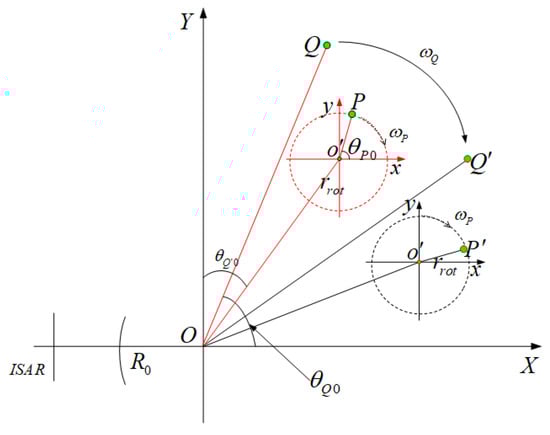
Figure 1.
ISAR geometric model.
The micro-Doppler effect is illustrated by the rigid body portion scattering point Q and the rotational scattering point P of the target in Figure 1. The echo signal after range compression is defined as
where A is the amplitude of the echo signal, is the pulse width, is the modulation rate, c is the velocity of light, is the wavelength of carrier frequency, and is the distance difference from scattering point Q to the radar displaced phase center and reference point O. and correspond to the frequency domain and slow time of the pulse compression result, respectively.
For the rigid scattering point Q,
where is the distance from the rigid rotation center to point Q, is the angle between the X axis and in coordinate , and . Based on the assumption of the uniform circular motion for point Q, it is centered at O with angular velocity in the coherent accumulative time.
Since the accumulation on cross-range is very small here, it has , . The Doppler frequency of Q is given by
For high-speed rotating scattering point P on target, while it has the same rotation center to point O as Q, another rotation with center point of moving parts makes it different. As in Figure 1, it has
where is the distance from to O, is the angle between the X axis and at zero time, and they have . Similarly, is the radius of the rotation of P, is the angle between the X axis and at zero time, and they are related as . In comparison to Q, one more rotation of P introduces a term of sinusoidal modulation to it’s Doppler frequency:
which is called m-D information.
In the above model of the m-D effect, in coherent accumulative time, rigid parts appear as superpositions of sinusoidal waves in ISAR’s cross-range. Then, moving parts add modulation. When there are scattering points in rigid parts, and in moving parts, the echo signal could be written as
where represents the components from rigid parts, and and are the amplitude and frequency of the cross-range Doppler signal for the pth scattering point, respectively. , and have the same meaning for moving parts, and is the m-D information.
Figure 2 shows the process of ISAR imaging.
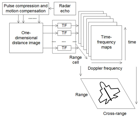
Figure 2.
The process of ISAR time-frequency imaging.
Originally, in the dotted line parts of Figure 2, signals from different range cells only need to do the Fourier transform then arrange results in order, the imaging result would then be obtained. In the frequency domain of those signals, the energy of the sinusoidal frequency modulated (FM) component brought by moving parts will be distributed in a range where the spectrum is larger than the rigid body component. In the final imaging results, they seemed to be unwanted interference information relative to the rigid body part. The Fourier transform only shows the distribution of these interferences in the frequency domain but does not indicate the information of these m-D components over time. In Figure 1, Fourier transform is replaced by time-frequency analysis, and the m-D information is reflected in a more specific form on the time-frequency plane.
3. Time-Frequency Analysis and S-Transform
Generally, time-frequency analysis methods can be divided into two categories: one-order time-frequency transform and second-order time-frequency distribution [12]. Although the latter works much better than the former for the single-component signals, it would bring cross-terms that are inconvenient to handle when processing multicomponent signals. As mentioned above, the signals used for imaging in this paper are multicomponent (6), so the time-frequency distribution method is not desirable. Thus, here we will start with the most basic short-time Fourier transform (STFT) in the one-order time-frequency transform.
The multicomponent (MC) FM signal is considered as
here is the phase function of the mth signal, and is the amplitude.
As the signal is inserted into the time-frequency plane by short time Fourier transform (STFT), we have
where is usually a Gaussian window function with fixed parameters. This would bring a fixed time-frequency resolution to the analysis result. Even if it is adjusted, it is difficult to get the overall optimality.
Similarly, the S-transform is defined as
and it holds a variable Gaussian window function.
For the component located in the low frequency region, the window function is longer and has better frequency resolution. The high-frequency area is the opposite, with better time resolution.
This feature matches the radar echo signal form (6) used for imaging in this paper: The better frequency resolution at low frequencies concentrates the energy of the rigid body component, while the better time resolution at high frequencies depicts the variation of the m-D component over time.
All of the above would make it possible for ST to get better results than STFT overall. In application, to keep the frequency resolution of the high frequency region, a lower bound should be set for the window length.
4. Synchrosqueezing Method
The results obtained from ST analysis are still somewhat insufficient: the energy would spread in the frequency direction of the high-frequency part, which affects the readability of the time-frequency map. Here, the synchrosqueezing method will be introduced for this problem. It is a post-processing method for time-frequency analysis results. The energy is compressed from the frequency direction, the final map is significantly improved, and the beneficial characteristics of the ST can be preserved.
If we consider a harmonic signal , its Fourier Transform is shown as
where is the Dirac-delta function. Hence, the S-transform of can be expressed as
This illustrates that are distributed into the ambiguity area in (9). Ideally, the frequency of is concentrated around . In practice, the energy of spreads out in a range of frequency. To eliminate the effect of modulated items, in the ST spectrum, the signal can calculate the instantaneous frequency (IF) whenever for any by
The form of the IF is suitable for S-transform [13]. Here, means is partial to t. By using (9), we can obtain . The multicomponent signals can be defined as a superposition of AM-FM components
where the and are, respectively, time-varying amplitude and phase functions satisfying and for any t. The goal is to recover the instantaneous frequencies and the instantaneous amplitudes . If there is some distance between the different components, i.e.,
where , it is called the well-separated multicomponent signal. can also perform effectively for IF estimation [14].
4.1. Synchrosqueezing S-Transform
Before introducing synchrosqueezing transform, it is necessary to revisit the reassignment technique (RM) [15]. The aim of RM is to sharpen the time frequency (TF) representation. There are two meaningful quantities that are called reassignment operators, and . The former is the same as Equation (14) and the latter is defined as
Here, means is partial to f. While RM as a useful post-processing technique that moves the coefficients according to the map in the TF plane, no mode reconstruction method is available.
Synchrosqueezing transform was originally introduced for analyzing auditory signals in [16] and developed further in [8]. It can be viewed as a special reassignment method. The coefficients are reassigned according to the map , making it remain invertible. The synchrosqueezing S-transform (SSST) is defined as follows:
where is an adjustable threshold.
By squeezing the frequency components within a certain range of instantaneous frequency, an energy-concentrated TF representation can be obtained. Then, the reconstruction of the original signal is computed by
where , and . is the complex conjugate of the Fourier transform of the mother wavelet .
More details of the proof can be found in [13].
4.2. Second-Order Synchrosqueezing S-Transform
Although SST gives a good TF representation and mode reconstruction for multicomponent signals, it is restricted to analysis signals made of weakly modulated modes [17]. For a mode , only when is approximate to zero or very small compared to , the instantaneous frequency estimation is close to . When considering the strong frequency-modulated signal, for instance a quadratic chirp, the is no longer negligible.
In order to deal with highly modulated signals like m-D components, second-order synchrosqueezing S-transform (SST2) was introduced by a more accurate IF estimate, based on the second-order operator. The operator corresponds to the second-order derivatives of phase . The second-order local complex modulation operator is defined as
where represents to t for second-order partial derivatives, and means that is partial to t and then partial to f. Owing to the operator, a more precise IF estimate can be obtained as
Then, the second-order synchrosqueezing S-transform (SSST2) is modified by replacing by in (15).
5. Numerical Experimental Results
For the sake of clarity, the abbreviations used below will be detailed here. They are S-transform (ST), short-time Fourier transform (STFT), synchrosqueezing transform (SST), synchrosqueezing S-transform (SSST), and second-order synchrosqueezing S-transform (SSST2).
In this section, the simulation experiment with adjustable parameters will be given first. Results are compared using different time-frequency analysis methods. Subsequently, the actual ISAR signal is also tested.
First, ISAR data is simulated on the helicopter miniaturization model in Figure 3. The simulation parameters are shown in Table 1. Its resolution will be more than enough for the target. Three different propeller speeds are set, which plays a decisive role in the performance of the m-D component.
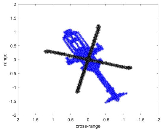
Figure 3.
ISAR geometric model.

Table 1.
Simulation parameters.
In Figure 4a,c, the imaging results using STFT and ST are respectively shown. Although both of them roughly represent the outline of the target rigid body part due to the setting of the experimental parameters, it is obvious that the ST subsection is more accurate and reflects some details. The reason can be seen from the time-frequency analysis results of the single distance unit (300th) using two methods: for the rigid body component, ST can obtain a more gradual result for the low-frequency part, while it would jitter in the STFT (Figure 4b,d).
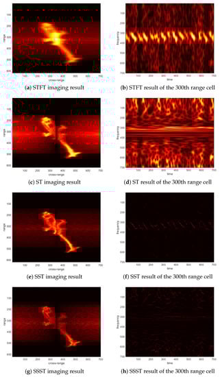
Figure 4.
Results of target with a main rotor speed of 5 r/s. ST—S-transform; SST—synchrosqueezing transform; SSST—synchrosqueezing S-transform; STFT—short time Fourier transform.
After applying the synchrosqueezing method, the imaging effects of both methods have been significantly improved. The SST imaging result (Figure 4e) is more concentrated, and the contour of the target becomes clearer. In the time-frequency map, the energy is concentrated in the low-frequency part, but the jitter of the rigid body component still exists (Figure 4f).
For relatively clear ST imaging results, the SSST changes are more reflected in the further depiction of the details (Figure 4g). Since the application of the ST changes the energy distribution of the signal in the frequency domain, the difference in energy between the rigid body imaging result and the m-D information is not as sharp as the SST result. But this also makes the m-D component not too weak (Figure 4h). In addition, in the results of SSST, the readability of the m-D component is also significantly improved, although this should mainly be attributed to ST. But the effect of the original ST in the high-frequency part is not ideal (Figure 4b).
When the rotational speed is increased to 10 r/s and 20 r/s, the same analysis results as those of Figure 4 are also correspondingly placed in Figure 5 and Figure 6.
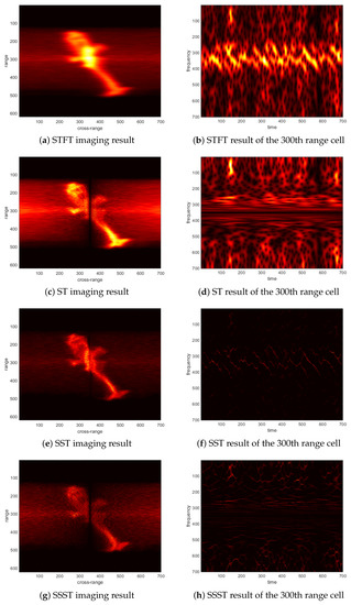
Figure 5.
Results of target with a main rotor speed of 10 r/s.
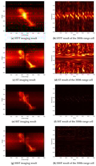
Figure 6.
Results of target with a main rotor speed of 20 r/s.
The difference between these results is the same as when the rotating speed is 5 r/s, but the m-D component brings more interference than before, which makes the imaging result blurred (Figure 5a,c,e,g and Figure 6a,c,e,g).
The characteristics of the results of each time-frequency analysis are not significantly different from the previous ones; the jitter range of the rigid body components of STFT and SST seems to be larger (Figure 5b,f and Figure 6b,f). In the results of ST and SSST, the energy is more distributed at high frequencies (Figure 5c,d,g,h). These changes become more pronounced after increasing the rotational speed to 20 r/s (Figure 6c,d,g,h).
After the second-order synchrosqueezing is further applied (Figure 7), it mainly affects the time resolution of the m-D separation in each time-frequency map (Figure 7b,d,f). This is easier to observe in the zoomed red rectangle region of Figure 6h and Figure 7f,g,h. The imaging result has no obvious gap (Figure 7a,c,e) with the SSST result.
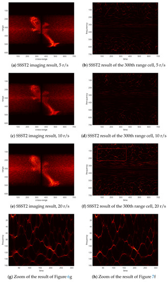
Figure 7.
Second-order synchrosqueezing S-transform (SSST2) results of target with different main rotor speed.
With simple energy accumulation criteria, the rigid body component can be roughly separated from the imaging results. The advantage of ST-based results (Figure 8b,d,f) relative to STFT (Figure 8a,c,e) is obvious. The former almost restored the details of the rigid part of the original model (Figure 3). It is worth mentioning that, although the contour of the rigid body part of the SSST2 imaging result is blurred at the rotational speeds of 10 r/s and 20/s (Figure 7c,e), the details of the extraction result can still be compared, with SST having a better performance (Figure 8d,f).
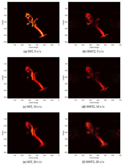
Figure 8.
Imaging separation results of simulated signals.
For the computing speed, SSST is not very different from the more complex SSST2, and the latter is even slightly faster (SSST: 1227s; SSST2: 934s). Moreover, due to the use of more matrix operations, SST is much faster than the other two methods (SST: 23s) that use more loop statements, as they hold similar levels of complexity. The above results show that there is still a lot of optimization space for the SSST and SSST2 programs used in this paper, and the calculation of operator (20) for SSST2 does not significantly change the computational complexity.
Actual An-26 aircraft data is also subjected to similar experiments. Similar to Figure 4, Figure 5 and Figure 6, Figure 9 shows the imaging effects of different methods (Figure 9a,c,e,g) and the time-frequency analysis results of a certain distance unit (Figure 9b,d,f,h). The difference between the results is still consistent with the previous simulation data. In addition, the imaging effects of SSST and SSST2 are still similar (Figure 9g and Figure 10a), and their differences are reflected in the time resolution of high-frequency components (Figure 9h and Figure 10b). For real data, STFT-based imaging is even worse; the more concentrated energy allows the latter to achieve a better separation result (Figure 11a,b).
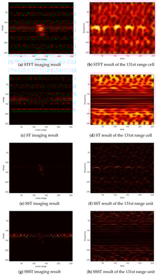
Figure 9.
Time-frequency and imaging analysis results of real An-26 data.
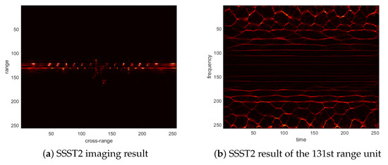
Figure 10.
Time-frequency and imaging analysis results of real An-26 data.
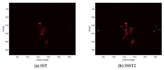
Figure 11.
Imaging separation results of real An-26 data.
6. Conclusions
In this paper, S-transform is applied to ISAR imaging. Since the multiresolution characteristics of S-transform and the characteristics of radar echo signals match each other, better analysis and imaging results are achieved compared with STFT; this contrast is obvious in both simulation and actual data results. In the simulated helicopter model, although the micro-Doppler component brings more interference to the imaging results as the rotational speed of the rotor increases, after the application of the synchrosqueezing method, the quality of the time-frequency analysis results is significantly improved. Especially in the ST-based synchronous compression results, the change in the micro-Doppler component over time in the frequency direction is clearly depicted. All of the above will play an important role in subsequent work such as feature extraction, parameter estimation, etc.
Author Contributions
The contributions of the authors are as follows. Data curation, B.Z.; Formal analysis, M.Z.; Funding acquisition, X.Z.; Investigation, L.Z.
Funding
This research was funded by National Natural Science Foundation of China grant number 61701374.
Conflicts of Interest
The authors declare no conflict of interest.
References
- Chen, V.C. Joint time-frequency analysis for radar signal and imaging. In Proceedings of the IEEE International Geoscience and Remote Sensing Symposium, Barcelona, Spain, 23–28 July 2007; pp. 5166–5169. [Google Scholar]
- Chen, V.C.; Li, F.; Ho, S.-S.; Wechsler, H. Analysis of micro-Doppler signatures. IEEE Proc. Radar Sonar Navig. 2003, 150, 271. [Google Scholar] [CrossRef]
- Chen, V.C.; Li, F.; Ho, S.-S.; Wechsler, H. Micro-Doppler Effect in Radar: Phenomenon, Model, and Simulation Study. IEEE Trans. Aerosp. Electron. Syst. 2006, 42, 2–21. [Google Scholar] [CrossRef]
- Luo, Y.; Zhang, Q.; Qiu, C.; Liang, X.; Li, K. Micro-Doppler Effect Analysis and Feature Extraction in ISAR Imaging With Stepped-Frequency Chirp Signals. IEEE Trans. Geosci. Remote Sens. 2010, 48, 2087–2098. [Google Scholar]
- Stankovi’c, L.J.; Stankovi’c, S.; Thayaparan, T.; Dakovi’c, M.; Orovi’c, I. Separation and Reconstruction of the Rigid Body and Micro-Doppler Signal in ISAR Part I—Theory. IET Radar, Sonar Navig. 2015, 9, 1147–1154. [Google Scholar] [CrossRef]
- Stankovi’c, L.J.; Stankovi’c, S.; Thayaparan, T.; Dakovi’c, M.; Orovi’c, I. Separation and Reconstruction of the Rigid Body and Micro-Doppler Signal in ISAR Part II—Statistical Analaysis. IET Radar Sonar Navig. 2015, 9, 1155–1161. [Google Scholar] [CrossRef]
- Stockwell, R.G.; Mansinha, L.; Lowe, R.P. Localization of the complex spectrum: The S transform. IEEE Trans. Signal Process. 1996, 44, 998–1001. [Google Scholar] [CrossRef]
- Daubechies, I.; Lu, J.; Wu, H.T. Synchrosqueezed wavelet transforms: An empirical mode decomposition-like tool. Appl. Comput. Harmon. Anal. 2011, 30, 243–261. [Google Scholar] [CrossRef]
- Brajovic, M.; Popovic-Bugarin, V.; Djurovic, I.; Djukanovic, S. Post-processing of Time-Frequency Representations in Instantaneous Frequency Estimation Based on Ant Colony Optimization. Signal Process. 2017, 138, 195–210. [Google Scholar] [CrossRef]
- Oberlin, T.; Meignen, S.; Perrier, V. Second-Order Synchrosqueezing Transform or Invertible Reassignment? Towards Ideal Time-Frequency Representations. IEEE Trans. Signal Process. 2015, 63, 1335–1344. [Google Scholar] [CrossRef]
- Pham, D.H.; Meignen, S. High-Order Synchrosqueezing Transform for Multicomponent Signals Analysis—With an Application to Gravitational-Wave Signal. IEEE Trans. Signal Process. 2017, 65, 3168–3178. [Google Scholar] [CrossRef]
- Sejdic, E.; Djurovic, I.; Jiang, J. Time-frequency feature representation using energy concentration: An overview of recent advances. Digit. Signal Process. 2009, 19, 153–183. [Google Scholar] [CrossRef]
- Huang, Z.; Zhang, J.; Zhao, T.; Sun, Y. Synchrosqueezing S-Transform and Its Application in Seismic Spectral Decomposition. IEEE Trans. Geosci. Remote Sens. 2016, 54, 817–825. [Google Scholar] [CrossRef]
- Thakur, G.; Wu, H.T. Synchrosqueezing-based Recovery of Instantaneous Frequency from Nonuniform Samples. Siam J. Math. Anal. 2010, 43, 2078–2095. [Google Scholar] [CrossRef]
- Auger, F.; Flandrin, P. Improving the readability of time-frequency and time-scale representations by the reassignment method. IEEE Trans. Signal Process. 1995, 43, 1068–1089. [Google Scholar] [CrossRef]
- Daubechies, I.; Maes, S. A nonlinear squeezing of the continuous wavelet transform based on auditory nerve models. In Wavelets in Medicine and Biology; CRC Press: Boca Raton, FL, USA, 1996; pp. 527–546. [Google Scholar]
- Auger, F.; Flandrin, P.; Lin, Y.T.; McLaughlin, S.; Meignen, S.; Oberlin, T.; Wu, H.-T. Time-Frequency Reassignment and Synchrosqueezing: An Overview. IEEE Signal Process. Mag. 2013, 30, 32–41. [Google Scholar] [CrossRef]


© 2019 by the authors. Licensee MDPI, Basel, Switzerland. This article is an open access article distributed under the terms and conditions of the Creative Commons Attribution (CC BY) license (http://creativecommons.org/licenses/by/4.0/).