Parallel Implementation on FPGA of Support Vector Machines Using Stochastic Gradient Descent

Abstract

Sequential Minimal Optimization (SMO) is the traditional training algorithm for Support Vector Machines (SVMs). However, SMO does not scale well with the size of the training set. For that reason, Stochastic Gradient Descent (SGD) algorithms, which have better scalability, are a better option for massive data mining applications. Furthermore, even with the use of SGD, training times can become extremely large depending on the data set. For this reason, accelerators such as Field-programmable Gate Arrays (FPGAs) are used. This work describes an implementation in hardware, using FPGA, of a fully parallel SVM using Stochastic Gradient Descent. The proposed FPGA implementation of an SVM with SGD presents speedups of more than 10,000× relative to software implementations running on a quad-core processor and up to 319× compared to state-of-the-art FPGA implementations while requiring fewer hardware resources. The results show that the proposed architecture is a viable solution for highly demanding problems such as those present in big data analysis.

1. Introduction

Areas such as image classification and bioinformatics can greatly profit from the use of artificial intelligence algorithms such as Support Vector Machine (SVM). However, because SVM is computationally costly, software applications often do not provide sufficient performance in order to meet time requirements for large amounts of data [1,2]. Hardware platforms such as Field-Programmable Gate Arrays (FPGAs) and Graphic Processing Units (GPUs) can be used to increase the performance of SVM implementations, resulting in a higher number of samples evaluated per second (throughput) compared to General Purpose Processors (GPPs). These platforms have been used for real-time and massive data mining applications, also called Mining of Massive Datasets. Although GPUs have higher performance than GPPs, FPGAs can provide a better alternative as they can achieve similar computational power while having lower energy consumption [1,2,3].

A widely used method for SVM training is Sequential Minimal Optimization (SMO). SMO is a technique to simplify the quadratic optimization problem involved in calculating the weights of the SVM [4]. In previous works, several classes of SVMs were implemented in FPGA, mainly relying on the use of the SMO algorithm for training.

Reference [5] implements the inference step of a SVM in FPGA for large datasets. As a form of validation, the MNIST dataset is used, achieving accelerations of up to 8× compared to GPU and FPGA implementations. The implementation proposed in [6] develops a cascade SVM implementation, based on an earlier system developed by the same authors. With this new implementation, the authors achieved a reduction of 25% in the number of logical elements used, a 2× increase in performance and a reduction of 20% in the peak power required in relation to their previous work.

Gradient-based methods can also be used to implement the SVM training step. However, some of these methods depend on the analysis of the complete training set before performing an update of the network weights. To improve SVM scalability regarding the size of the data set, Stochastic Gradient Descent (SGD) algorithms are used, as a simplified procedure for evaluating the gradient of a function [7].

It is still possible to contribute to the literature exploring the use of the FPGA to implement SVMs trained with the SGD algorithm. Currently, works focus on large scale SGD implementations as in [8], which integrates the Spark framework, making use of a SGD implementation in FPGA to accelerate the training step of a linear SVM. For validation, the implementation was used for the classification of 7500 cancer cells images of size 256 × 256, achieving an increase in throughput of up to 2× compared to an implementation on a cluster of computers.

Other approaches focus on building a scalable SGD accelerator [9]. In their work, the impact of quantization on statistical and hardware efficiency are discussed and how the use of stochastic quantization and fixed-point arithmetic can lead to better convergence than naive quantization. The implementation presented uses an embedded CPU that transmits the training samples to the FPGA.

In [10] the authors developed an implementation of the HogBatch algorithm in hardware based on systolic arrays, and used an extension of SGD that allows batching. Reference [11] evaluates the impact on communication and computation time of low-precision, asynchronous SGD using both CPU and FPGA implementations. Moreover, they present a new model to describe SGD implementations called Dataset, Model, Gradient, Communications (DMGC).

This paper presents a proposal to implement Parallel Support Vector Machines, with training performed by the stochastic gradient descent technique in reconfigurable hardware using FPGA. As an alternative to reach higher throughput, hardware resource optimization techniques such as different numerical representations are explored. Once the implementations have been made, an analysis of the occupied resources and other hardware performance parameters is performed. The experimental results are obtained with a Xilinx Virtex-6 XC6VCX240T-1 FPGA.

The rest of the paper is organized as follows. Section 2 describes how the SVM has been implemented and the equations that describe it. Section 3 defines the computational platforms used, how the SVM training was performed and how the results were obtained. Section 4 analyses and compares the results obtained by the implementations in software and hardware. Section 5 compares the results obtained with the state of the art regarding throughput. Section 6 provides an overview of what was discussed and summarizes the contributions of the paper.

2. Project Description

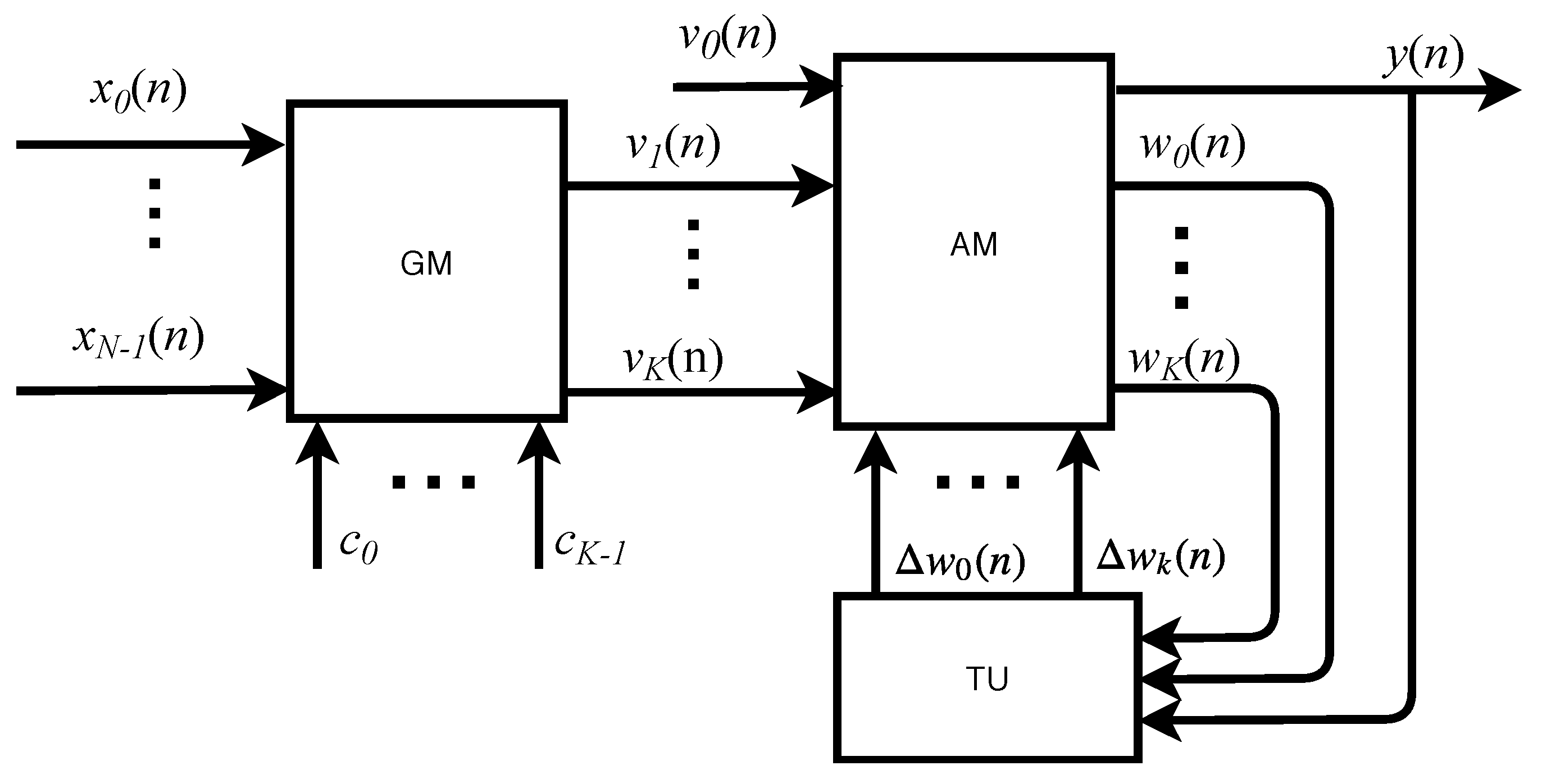
A high-level description of the system can be made based on three main structures; Gaussian Module (GM), Aggregation Module (AM) and Training Unit (TU), as shown in Figure 1. The GM is responsible for mapping the input into a different representation space, easing the classification of non-linearly separable patterns. The AM receives the GM output and, based on its weights, maps them to one of the possible labels. Finally, TU implements the SGD algorithm and adjusts the AM weights. In the following subsections, the modules will be detailed. The structures GM, AM and TU processes all the information in each n-th sample time, $t_s$, in other words, at every $t_s$ seconds there is a new output $y\left(n\right)$ from the N inputs $x_i\left(n\right)$ {$i=0,\cdots ,N-1$}, and the $K+1$ weights $w_j\left(n\right)$ {$j=0,\cdots ,K$} are updated. As this proposal is a full parallel implementation, the sample time, $t_s$, is also the iteration time and n indicates the current iteration. The SVM throughput, $th$, in samples per second (sps) or in iterations per second (ips) can be expressed as

$$th=1/t_s.$$

(1)

Figure 1. High-level system.

2.1. Gaussian Module (GM)

In this module, the entries are mapped into another representation space see Figure 1, to facilitate the classification of non-linearly separable patterns by the SVM. The mapping is done through the use of kernels. Allowing to transform the input space of N into a space of K dimensions. In this work, it was implemented the Gaussian, also called Radial-Basis Function (RBF), kernel which can be expressed as

$$v_j\left(n\right)=e^{\frac{dis{t}_j\left(n\right)}{2{\sigma }^2}}=e^{\frac{{\sum }_{i=1}^K{(x_i\left(n\right)-c_{ji}\left(n\right))}^2}{2{\sigma }^2}}$$

(2)

where $c_{ji}\left(n\right)$ is the j-th center of the gaussian function associated with the i-th input, $x_i\left(n\right)$ the i-th input, ${\sigma }^2$ the variance of each kernel function, $dis{t}_j\left(n\right)$ the j-th distance from each input to the center, $v_j\left(n\right)$ the j-th exit of GM in the n-th iteration and $v_0\left(n\right)$ the bias.

To maximize the throughput of the system and reduce computation time of Equation (2), most operations are executed in parallel. With the exception of summation, which is executed using a tree adder. To reduce resource consumption and decrease execution time in the FPGA, the exponential function is implemented through the use of Look-Up Tables (LUTs), where each address of the LUT stores a value of the exponential. This implementation choice implies in a delay of one sample in the algorithm execution. However, the impact on throughput is lower than if the exponential function was implemented using specific hardware circuitry.

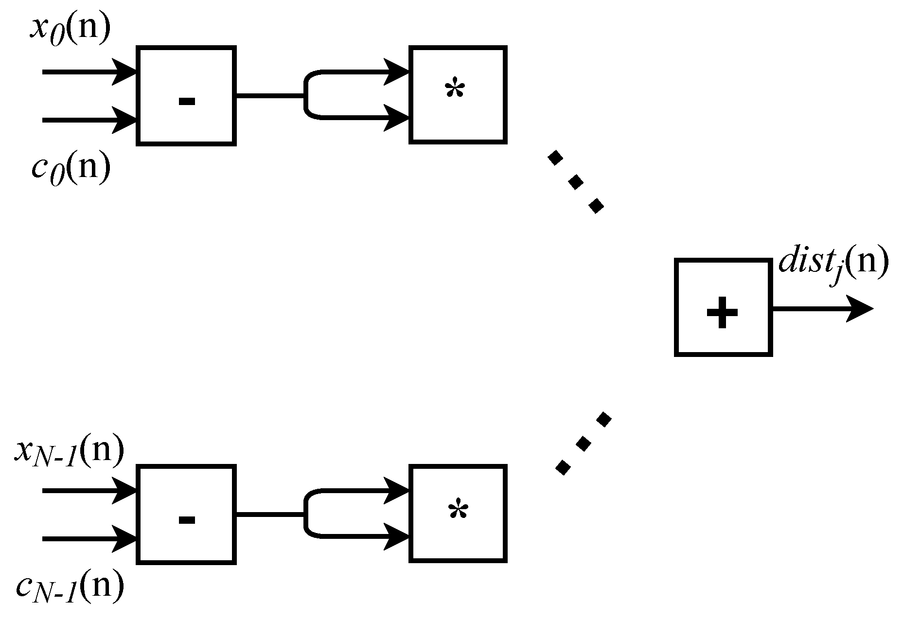
The j-th distance $dis{t}_j\left(n\right)$ shown in Equation (2), is computed in parallel as in Figure 2. It is important to note that all arithmetic operations are performed in parallel which increases performance regarding throughput.

Figure 2. Distance computation.

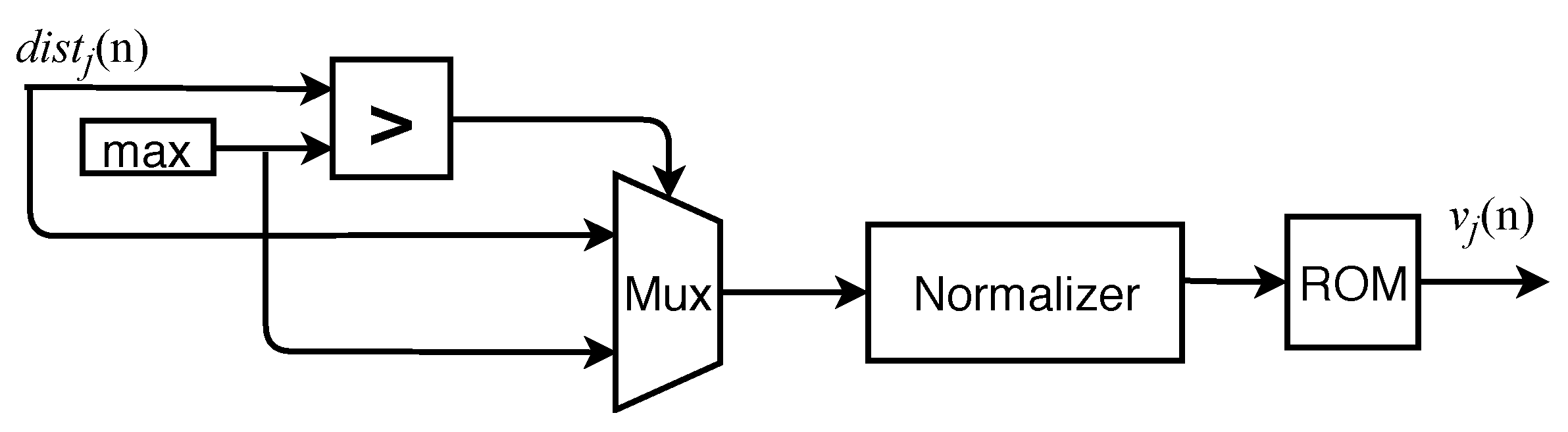
Having the value of $dis{t}_j\left(n\right)$, the calculation of the Equation (2) is done using Read-Only Memory (ROM), composed of LUTs of depth 9. The circuit to convert the distance to memory addresses is illustrated in Figure 3. Being $max$, the upper edge of the function domain and normalizer the circuit responsible for converting from distance metric to memory address. To discretize the gaussian a maximum value for the distance of 4 and a minimum of 0 was considered. Within that range the gaussian was evaluated at steps of $0.01$ and the values were stored on the ROM memory, which resulted in 401 values being stored. The normalizer then divides the output of the mux with the discretization step.

Figure 3. Kernel computation.

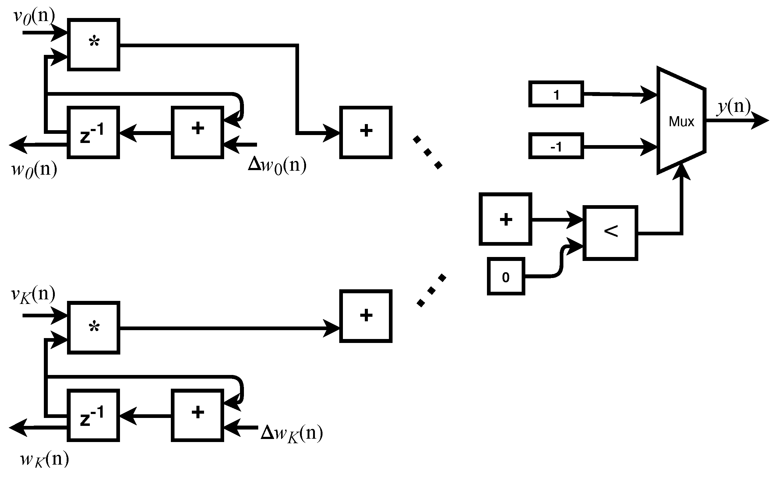
2.2. Aggregation Module (AM)

After the N entries are mapped into a new space, the AM is used to classify the entries $v_j\left(n\right)$. In this implementation, only binary classification is possible, which consists of classifying the input vector into one of two possible classes [12]. The classes are represented by 1 and $-1$. The classification is expressed as

$$y\left(n\right)=sgn\left(\sum _{j=0}^K\left(v_j\left(n\right)w_j\left(n\right)\right)\right)$$

(3)

where $w_j\left(n\right)$ is the neural weight associated with the j-th input, and $y\left(n\right)$ the SVM output in the n-th iteration. The implementation of this equation in the FPGA is shown by Figure 4. For this to happen the entries $v_j\left(n\right)$ are multiplied in parallel by their corresponding weights $w_j\left(n\right)$, the result is then summed using a tree adder.

Figure 4. Aggregation module.

2.3. Training Unit (TU)

TU implements the equations expressed as

$$w_j(n+1)=w_j\left(n\right)+\Delta w_j$$

(4)

and

$$\Delta w_j=\{\begin{array}{ll}\eta \lambda w_j\left(n\right),& \mathrm{if}y\left(n\right)d\left(n\right)\ge 1\\ \eta (v_j\left(n\right)y\left(n\right)-\lambda w_j\left(n\right)),& \mathrm{if}y\left(n\right)d\left(n\right)otherwise\end{array}$$

(5)

where $d\left(n\right)$ is the desired output, $y\left(n\right)d\left(n\right)\ge 1$ are the correctly classified results, $\eta$ is the learning rate and $\lambda$ is the regularization parameter. The variable $\lambda$ specifies how much the training samples are sufficient to specify a solution to the problem. When $\lambda \to \infty$, it means that the data is not trustworthy and $\lambda =0$ otherwise [13].

For Equations (4) and (5), the loss function chosen was Hinge-Loss and the regularization given by the $l_1$ method [14]. In this work, a variant of the Pegasos algorithm was implemented for training [15]. The designed circuit is presented in Figure 5.

Figure 5. Training unit.

3. Methodology

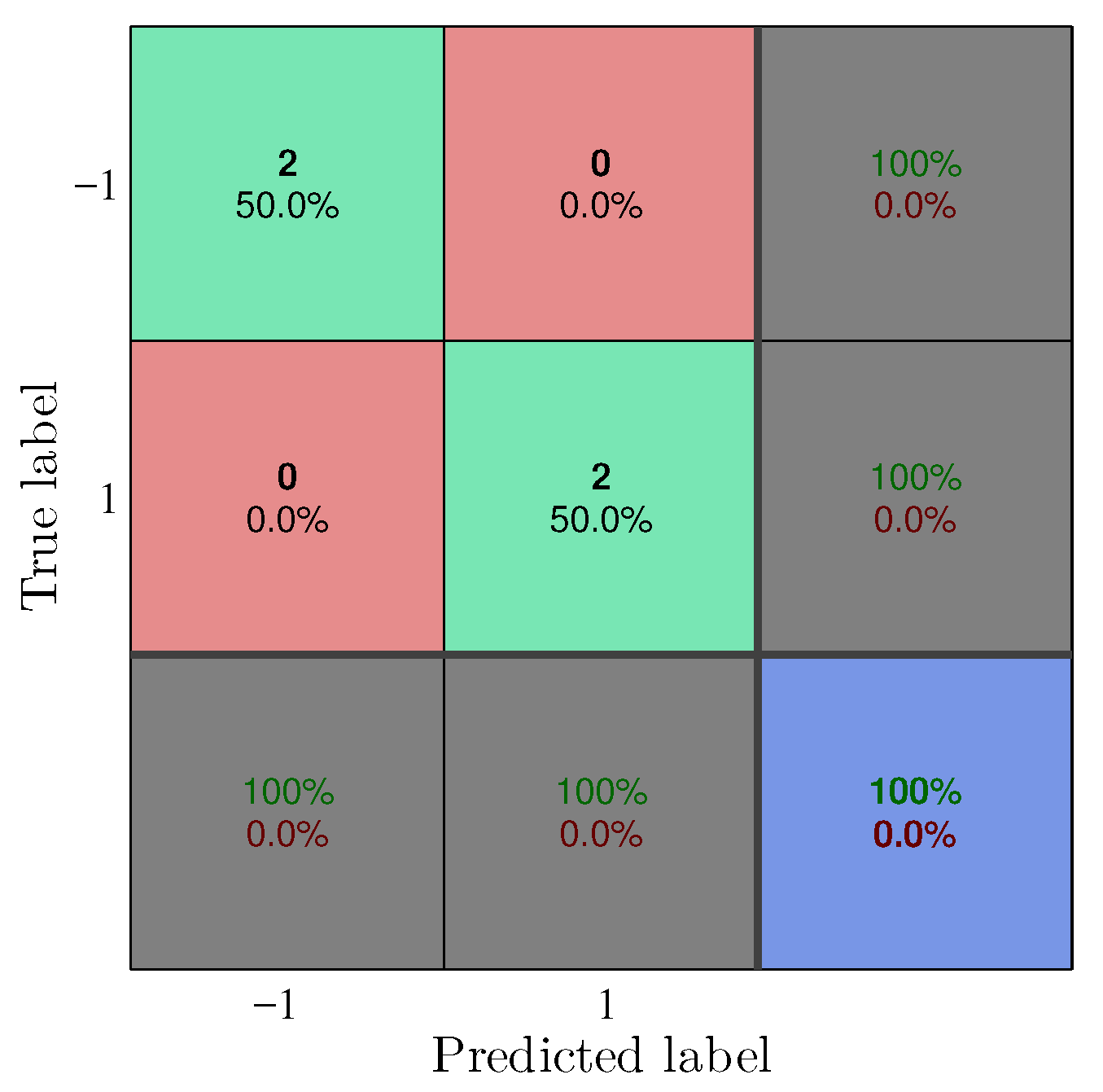
Two datasets were used to validate the hardware design. The first was the XOR gate, being the SVM used to draw the ideal decision surface that divides the two classes correctly. In this design, the value of each j-th input, $x_j\left(n\right)$, in the n-th instant (or iteration), corresponds to the input of the XOR gate and $y\left(n\right)$ the output of the circuit.

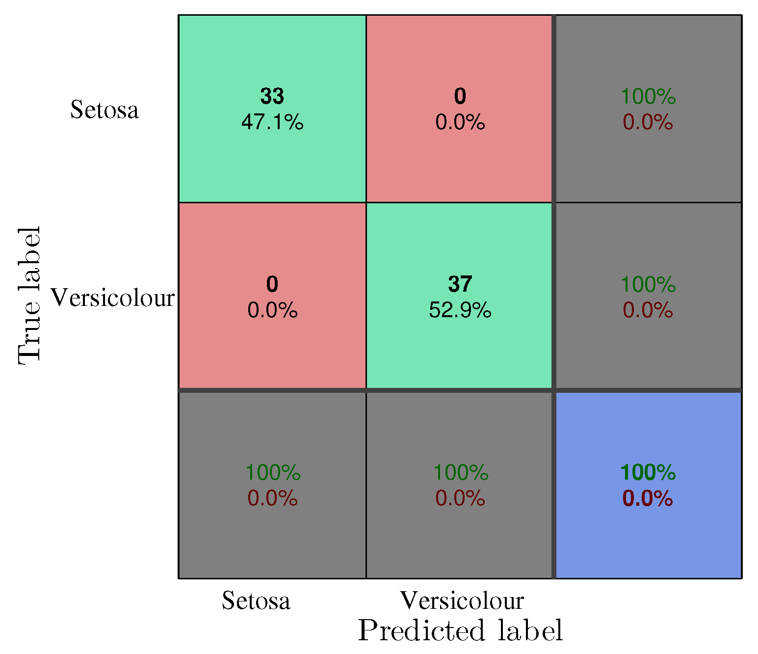
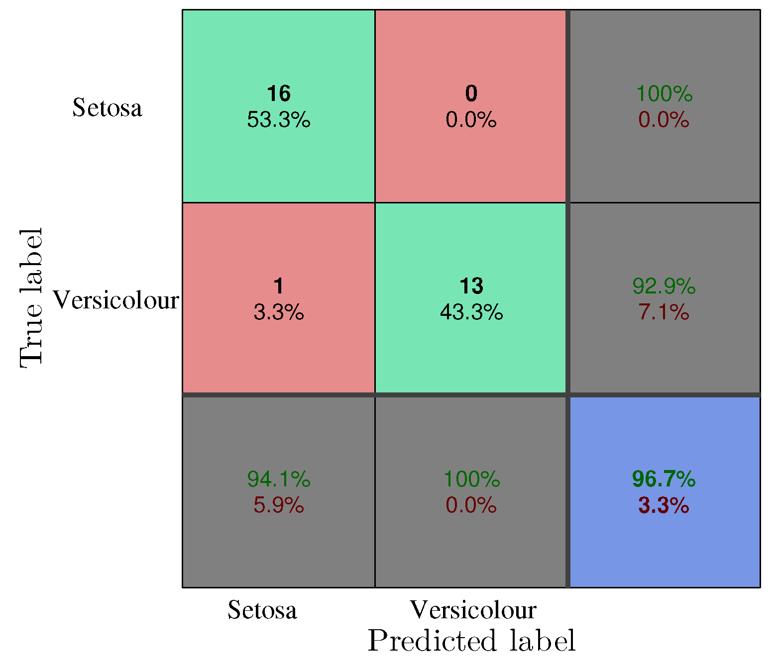
The second set of data is from the Iris flower, described in [16]. Where each input $x_j\left(n\right)$ corresponds to the value of the length and width of the sepal and the petal. This dataset was made with the aim of classifying three types of flowers from the Iris family; Iris Setosa, Versicolor and Virginica. This implementation restricts to only classify Iris Setosa and Versicolor because the SVM used is a binary classifier. For this reason, all data related to Iris Virginica was removed from the dataset.

The results of the hardware design were then compared to the software implementation in Python using the scikit-learn package [17]. Python and scikit-learn were used since they are widely used tools in Data Science and AI. The software implementation uses double-precision floating-point format, while the hardware uses single-precision floating and fixed-point representation, the fixed-point representation uses 5 bits in the integer part and 20 in the fractional part. Although the software implementation does not use single-precision float pointing format according to [18] there is at most a speedup of 4 times between these numerical representations, depending on the instruction executed. With this experiment it was possible to acquire execution time data and usage of FPGA hardware resources.

Before the results were obtained, the dataset was preprocessed, which consisted of the separation between training and test set and in obtaining the centers of the kernels. In the case of the XOR gate, the training set is the same as the test set. For the Iris dataset, the samples were divided into $30\%$ for testing and $70\%$ for training. This was done randomly by the method train_test_split, also present in the scikit-learn package.

To obtain the centers of the kernels two methods were used. For the XOR dataset the centers were set using knowledge on the problem to find the ideal values. In the case of Iris dataset, the centers were calculated by the K-means algorithm, implemented by the KMeans class of the scikit-learn package. Once this data is retrieved in the Python environment, it is saved in CSV format to be used by the hardware implementation.

To execute the implementation in Python, a system with an i7 quad-core processor, running at 2.5 GHz with 8 GB of RAM and Python 3.6 was used. The RBF_kernel class was employed to map the SVM entries, using the RBF kernel and the class SGDClassifier was used to adjust the SVM parameters based on the SGD algorithm. This approach was necessary as Scikit-learn did not provide an implementation of kernel-based SVM using the SGD algorithm. The CPU time was measured taking the average of 10,000 executions of the algorithm, using the function_time function.

The hardware implementation was done through a Xilinx tool, called System Generator [19]. With it, is possible to create RTL circuits in Matlab Simulink and perform simulations with bit-level precision, making possible to create highly efficient circuits and also to easily interface with the Matlab programming environment. Our design was synthesized to a Xilinx Virtex-6 XC6VCX240T-1 FPGA containing 241,152 logic cells, 768 embedded multipliers and 37,680 slices [20], included on the ML605 evaluation board [21].

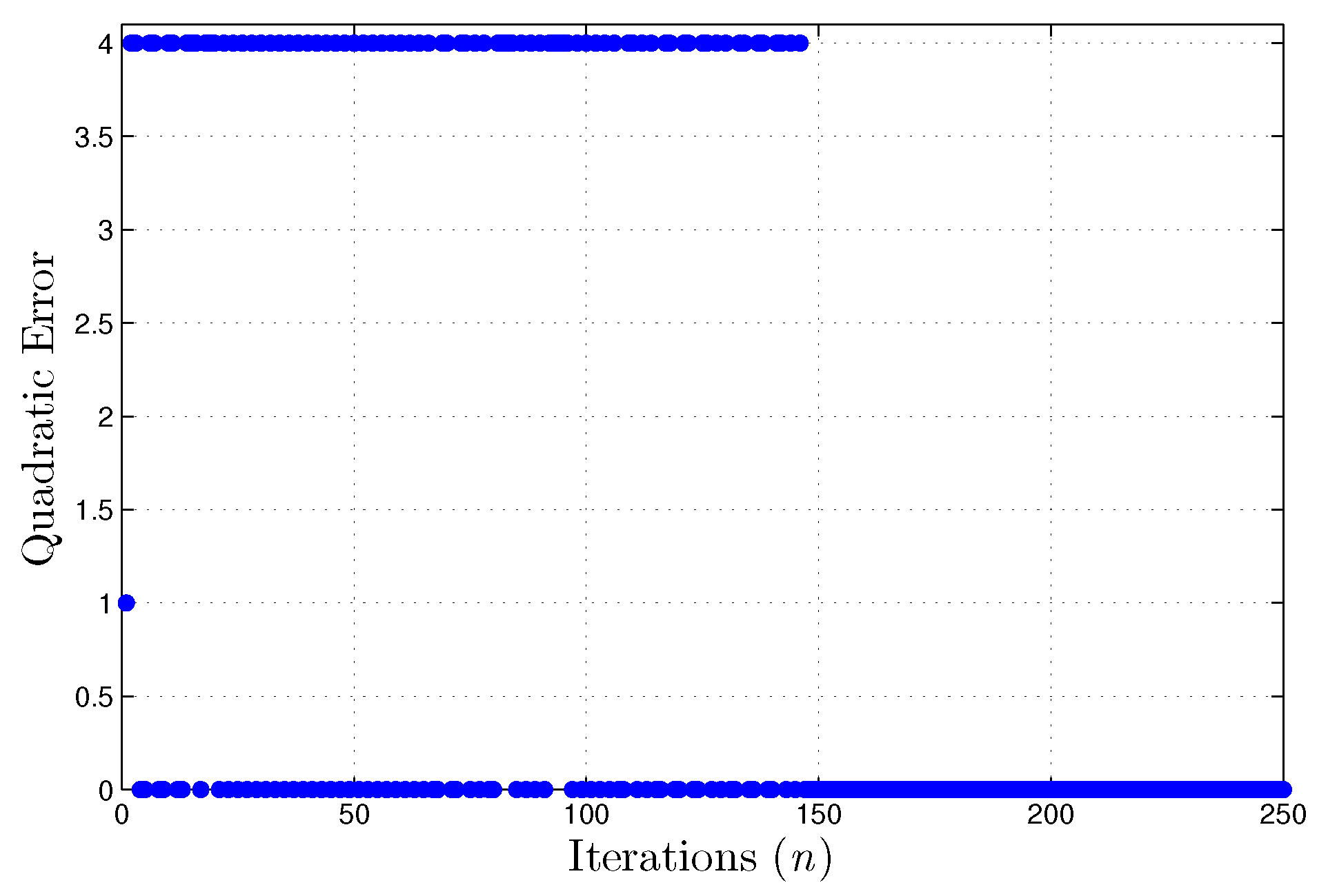
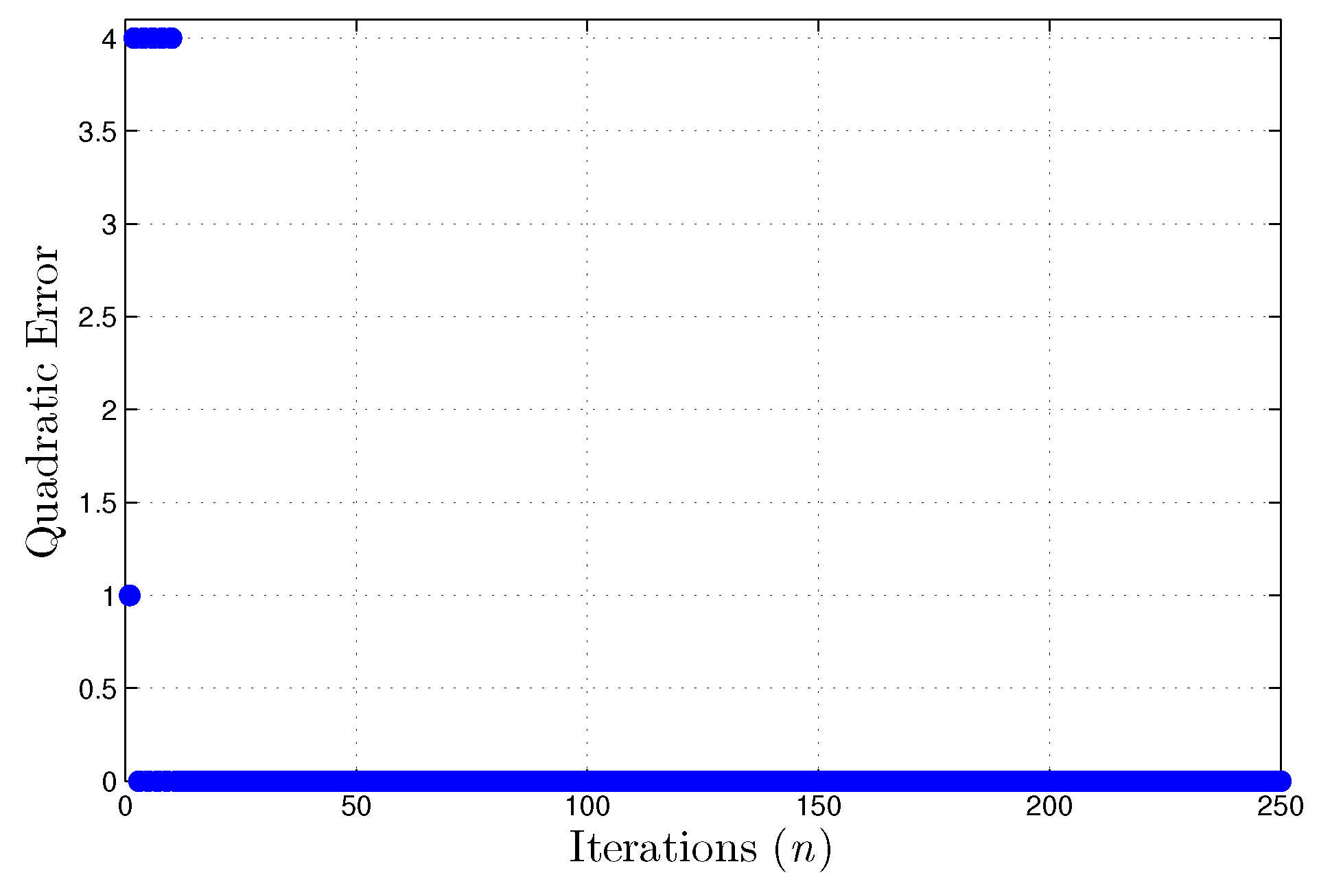
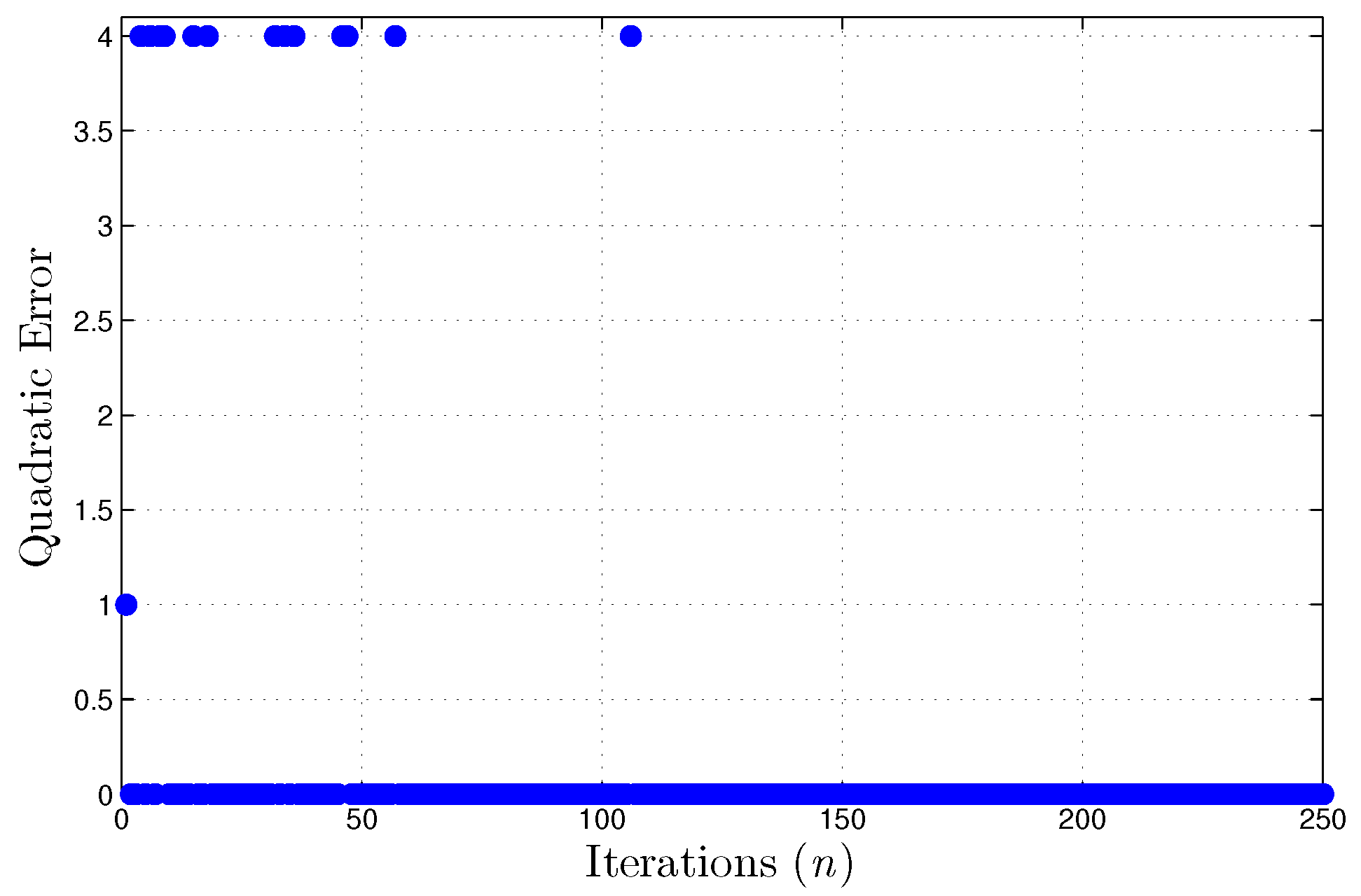
To validate the results of the software implementation a confusion matrix was drawn, in which the horizontal axis represents the classes predicted by the SVM and the vertical the correct classes. To generate the confusion matrix, results from the training and test sets were retrieved, making possible to analyze the learning and generalization capacity of the SVM. Regarding the hardware implementations, the evolution of the instantaneous quadratic error during training was analyzed, to facilitate the visualization of the results a window of 250 iterations is used to visualize the error.

4. Results

4.1. XOR Gate Dataset

4.1.1. Software Validation

In order to assess the capability of the software implementation on the scikit-learn package to correctly classify the samples on the dataset, a confusion matrix was used. With the results from the confusion matrix it is possible to validate the software implementation and use it to compare with the results obtained in hardware.

In the Figure 6, the first two green cells on the main diagonal show the number and percentage of correct classifications by the algorithm. From the total of 4 samples, 2 are correctly classified as class $-1$, this corresponds to $50\%$ of all samples. Similarly, 2 samples are correctly classified as 1, what corresponds to $50\%$ of the samples. The last cell on the main diagonal represents the total percentage of correct and incorrect classifications, for this dataset $100\%$ of the classes were correctly classified.

Figure 6. Confusion matrix of the XOR training, software implementation.

The first two red cells on the antidiagonal represent the percentage of incorrectly classified classes from the algorithm. From the total amount of samples, $0\%$ were wrongly classified. The first two grey cells from the last column represents the percentage that a class was correctly and wrongly predicted, both $-1$ and 1 classes were correctly predicted $100\%$ of the times. On the first two grey cells from the last row, is presented the percentage of times that a class that was outcomed by the algorithm was in fact that actual class in the dataset and the percentage it was not. In this dataset the algorithm outcomes the correct class $100\%$ of the times.

4.1.2. Floating Point Hardware

To analyze the hardware implementation, requirements such as execution time and use of available hardware are of great importance. In the case of FPGAs the resources are measured through the use of LUTs, Registers, Slices and Digital Signal Processors (DSPs) units, to name a few. Regarding the floating point implementation made for the XOR gate dataset, the resource consumption can be observed on Table 1.

Table 1. Resource utilization of the XOR gate dataset—floating point.

Number of Kernels	Registers	LUTs	Slices	DSP48
2	269	9135	3078	69
4	270	14,540	4654	102
8	470	27,614	9742	186
16	870	53,679	18,036	354

It can be seen that with 16 kernels the design occupies approximately $50\%$ of the LUTs available in the FPGA. As for the execution time, shown on Table 2 it can be noted that the FPGA implementation has a much shorter execution time than that presented in software. This increase in execution speed provides a significant increase in the number of samples that can be analyzed per second, as shown on the Table 3.

Table 2. Execution time, $t_s$, of the XOR gate dataset—floating point.

Number of Kernels	Software	Floating Point Hardware	Speedup
2	$0.518$ ms	$94.285$ ns	5462
4	$0.515$ ms	$120.701$ ns	4266
8	$0.513$ ms	$\mathrm{235,276}$ ns	2180
16	$0.508$ ms	$375.323$ ns	4266

Table 3. Throughput, $th$, of the XOR gate dataset—floating point.

Number of Kernels	Software	Floating Point Hardware
2	$1.930$ Ksps (Kips)	$10.5$ Msps (Mips)
4	$1.941$ Ksps (Kips)	$8.2$ Msps (Mips)
8	$1.949$ Ksps (Kips)	$4.2$ Msps (Mips)
16	$1.968$ Ksps (Kips)	$2.6$ Msps (Mips)

As for the correctness of the implementation in hardware, it can be seen through Figure 7 that the implementation converges in few iterations. Being the vertical axis is the value of the instantaneous quadratic error and the horizontal the number of iterations.

Figure 7. Quadratic error during training using the XOR dataset, floating point implementation.

4.1.3. Fixed-Point Hardware

As seen on Table 4, the fixed-point implementation is considerably more efficient than the floating point, using nearly $10\times$ fewer LUTs and slices. A better result is also obtained considering runtime, as shown on Table 5. Fixed-point implementation achieved a throughput approximately $5\times$ larger than floating point, generating a substantial increase in the number of samples analyzed per second, see Table 6. Although the reduced numeric precision in this design, the fixed-point implementation also converges in few iterations, as shown in Figure 8.

Table 4. Resource utilization of the XOR gate dataset—fixed point.

Number of Kernels	Registers	LUTs	Slices	DSP48
2	75	716	206	48
4	125	1266	364	84
8	225	2366	682	156
16	425	4566	1311	300

Table 5. Execution time, $t_s$, of the XOR gate dataset—fixed point.

Number of Kernels	Software	Fixed Point Hardware	Speedup
2	$0.518$ ms	$50.756$ ns	10,205
4	$0.515$ ms	$51.188$ ns	10,060
8	$0.513$ ms	$61.480$ ns	8344
16	$0.508$ ms	$63.367$ ns	8016

Table 6. Throughput, $th$, of the XOR gate dataset—fixed point.

Number of Kernels	Software	Fixed Point Hardware
2	$1.930$ Ksps (Kips)	$19.7$ Msps (Mips)
4	$1.941$ Ksps (Kips)	$19.2$ Msps (Mips)
8	$1.949$ Ksps (Kips)	$16.2$ Msps (Mips)
16	$1.968$ Ksps (Kips)	$15.7$ Msps (Mips)

Figure 8. Quadratic error during training using the XOR dataset, fixed point implementation.

4.1.4. Analysis

The Hardware implementations generated a large increase in the SVM training execution speed, as seen on Table 2 and Table 5. Moreover, the impact of the acceleration provided becomes even clearer when analyzing speedup, that is, how many times faster the hardware implementation is in relation to the software implementation. The acceleration value is obtained by dividing the runtime value in software by the runtime value on FPGA.

It can be seen that the use of FPGA decreased execution time by more than three orders of magnitude, reaching an increase in the execution speed of up to 10,$205\times$ compared to the implementation in Python. This higher execution speed provided by the reconfigurable hardware implementation is an important factor considering the amount of data presented in massive data analysis.

It is possible to draw a superior margin on the floating point hardware implementation execution speed, analyzing around 10 million samples per second. Since each sample consists of 8 bytes, it would be possible to compute 1 GB of information in at least $12.5$ s using 2 kernels. On fixed-point, with the same number of kernels, it is possible to analyze more than 19 million of samples of $4.5$ bytes per second, resulting in the analysis of 1 GB in at least $5.8$ s. Meanwhile, the implementation of Python would take about 1 hour to analyze the same amount of data.

Despite the increased throughput, the speed of floating-point hardware design decreases significantly with the number of kernels used. This is caused by the increase in the sum tree depth on the AM. However, this effect can be reduced by applying pipeline to each of the sum stages, adding a delay in the circuit response but increasing the SVM throughput.

4.2. Iris Dataset

4.2.1. Software Validation

Following the analysis presented for the Xor dataset, in Figure 9 the confusion matrix for the training samples of the Iris dataset is shown. From the total of 70 samples, 33 are correctly classified as Setosa, this corresponds to $47.7\%$ of all samples. Similarly, 37 samples are correctly defined as Versicolour, what corresponds to $52.9\%$ of the samples. For this dataset $100\%$ of the samples were correctly classified.

Figure 9. Confusion matrix of the Iris training, software implementation.

Regarding the percentage of times the Setosa and Versicolour classes were classified, the algorithm predicts them correctly $100\%$ of the times. Moreover, when accounting for the rate that a class that was outcomed by the algorithm was in fact that actual class in the dataset and the rate per cent it was not. In the training samples the algorithm outcomes the correct class $100\%$ of the times.

For the test samples retrieved from the Iris dataset the confusion matrix is presented on Figure 10. From the total of 30 samples, 16 were classified correctly as Setosa, amounting for $53.3\%$ of all samples. From the Versicolour class 13 samples are correctly classified, corresponding to $43.3\%$ of the samples. For this dataset $96.7\%$ of the classes were correctly classified.

Figure 10. Confusion matrix of the Iris test, software implementation.

The algorithm classified a sample from the Setosa class correctly $100\%$ of the times and from the Versicolour $92.9\%$ of the times. For the test samples the algorithm defines the Versicolour $100\%$ when it was the correct class, and Setosa $94.1\%$.

4.2.2. Floating Point Hardware

The use of hardware resources by the floating-point implementation is described on Table 7. Showing similar usage of resources to the XOR dataset, the runtime is also similar between the two sets of data as seen on Table 8. Generating a large number of analyzed samples per second as illustrated on Table 9. As occurred in the XOR dataset, to verify the correctness of the implementation, we see the error curve present in the Figure 11. From this, it is possible to realize that even for more complex problems such as the Iris dataset, the implementation in hardware can converge in a small number of iterations.

Table 7. Resource utilization of the Iris dataset—floating point.

Number of Kernels	Registers	LUTs	Slices	DSP48
2	174	10,816	3823	72
4	278	20,399	6902	126
8	486	39,594	14,017	234
16	1088	77,977	25,790	450

Table 8. Execution time, $ts$, of the Iris dataset—floating point.

Number of Kernels	Software	Floating Point Hardware	Speedup
2	$0.641$ ms	$90.982$ ns	7045
4	$0.628$ ms	$110.152$ ns	5701
8	$0.619$ ms	$132.055$ ns	4687
16	$0.620$ ms	$176.004$ ns	3641

Table 9. Throughput, $th$, of the Iris dataset—floating point.

Number of Kernels	Software	Floating Point Hardware
2	$1.560$ Ksps (Kips)	$10.99$ Msps (Mips)
4	$1.592$ Ksps (Kips)	$9.07$ Msps (Mips)
8	$1.615$ Ksps (Kips)	$7.57$ Msps (Mips)
16	$1.612$ Ksps (Kips)	$5.68$ Msps (Mips)

Figure 11. Quadratic error during training using the Iris dataset, floating point implementation.

4.2.3. Analysis

As done for the XOR gate dataset, the speedup provided by the hardware implementation is analyzed, see Table 8. The hardware implementation generated an increase of up to 7045× on SVM training speed. When evaluating the Table 9, it is noticed that the hardware implementation can analyze nearly $10.9$ million samples per second. Since each sample consists of 16 bytes, it would be possible to analyze 1 GB of information in up to $5.68$ s using 2 kernels.

5. Comparison with the State of the Art

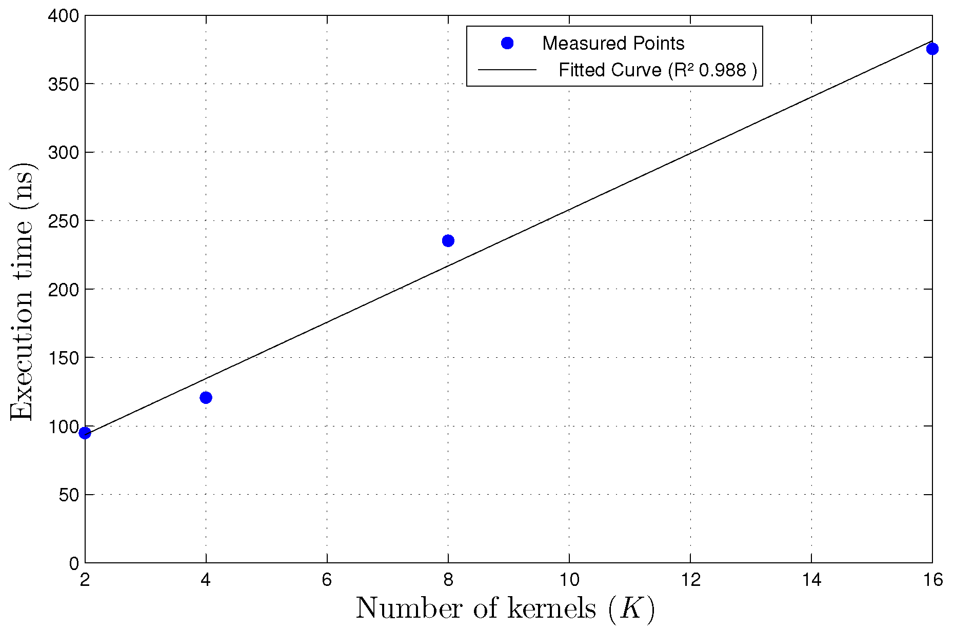
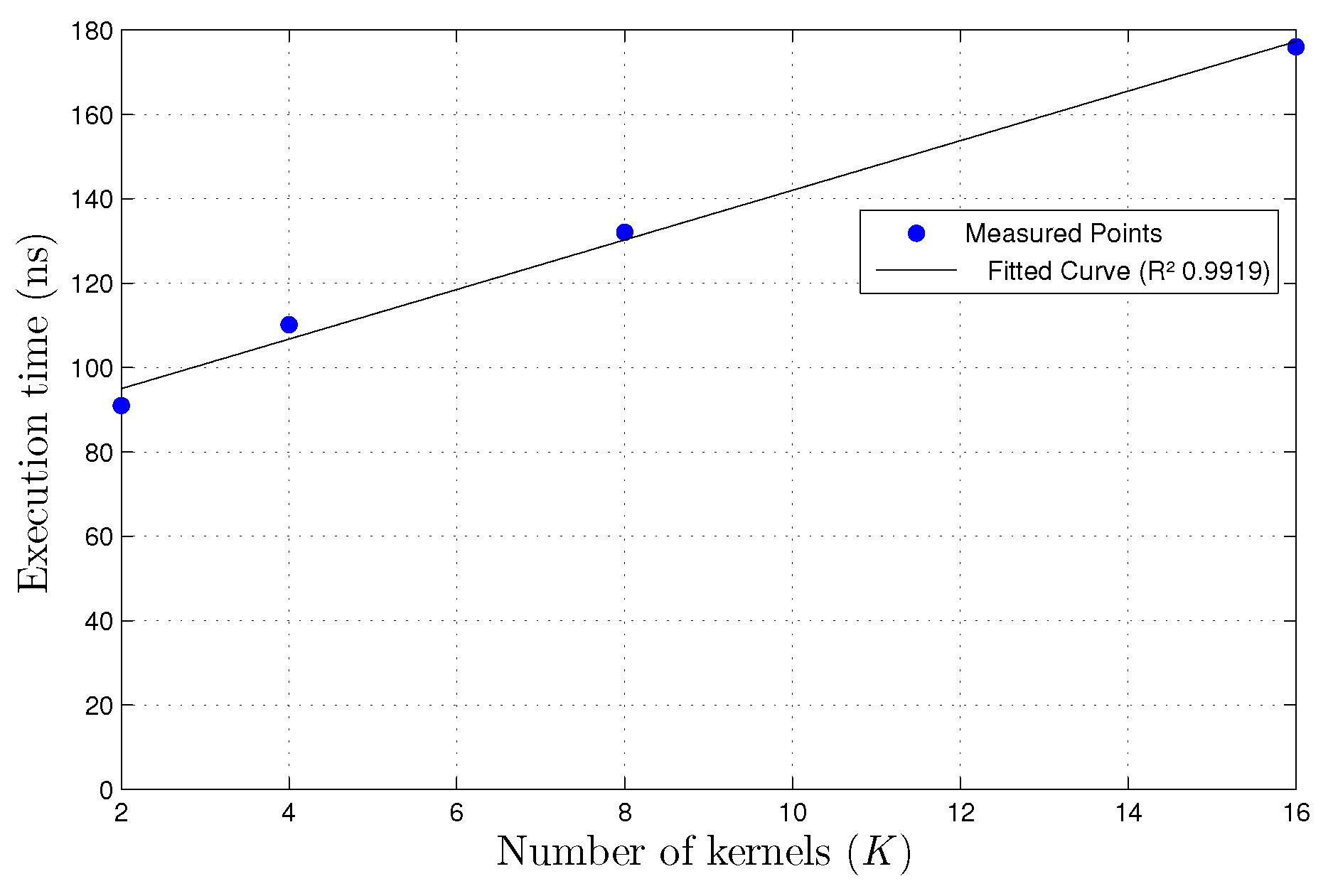
Although it was not possible to synthesize the design for a dataset with more than 4 features to compare with the state of the art, the results from the current datasets were extrapolated using a linear regression. The extrapolation was performed using data from the XOR dataset on both fixed and single precision floating point, as well as from Iris dataset using single precision floating point. The regressor has as input the number of kernels and as output the execution time. In order to compare to a model with 758 inputs, for example, the input of our regressor was 758, then the output was compared with the execution time of the model being referenced. Despite the fact that is not necessarily the case to have one kernel for each input, this draws a lower bound on our results. Further studies can show that the actual performance is different from the results presented in this work. As presented on Figure 12 the linear regression of the xor dataset using floating-point precision had a $R^2$ score of $0.988$, with sample time, $t_s$, computed as

$$t_s=20.566\times K+52.364.$$

(6)

Figure 12. Linear regression curve for execution time per sample for varing numbers of kernels k, XOR dataset floating-point precision.

For the implementation on the XOR dataset using fixed-point precision, the $R^2$ value is $0.8061$ as shown on Figure 13, the equation representing the sample time of the design is

$$t_s=0.9656\times K+49.456.$$

(7)

Figure 13. Linear regression curve for execution time per sample for varing numbers of kernels k, XOR dataset fixed-point precision.

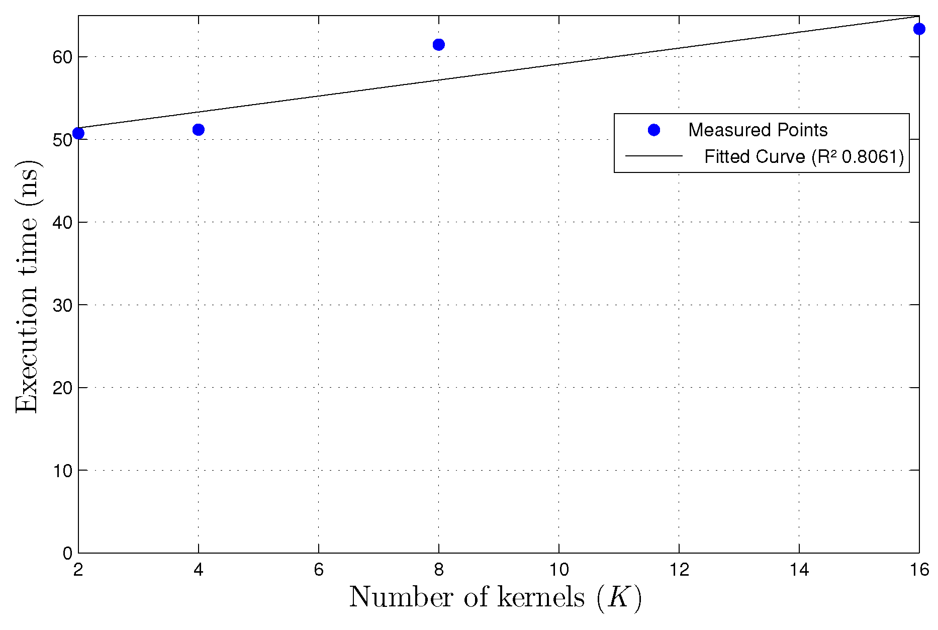
On the Iris dataset, using floating-point precision a $R^2$ value of $0.9919$ was achieved, as depicted on Figure 14 and having the following fitting curve

$$t_s=5.8794\times K+83.203.$$

(8)

Figure 14. Linear regression curve for execution time per sample for varing numbers of kernels k, Iris dataset floating-point precision.

The comparisons with the state of the art are summarized on Table 10.

Table 10. State of the art comparison.

Work	FPGA Used	Numerical Format	Model	Speedup XOR Float-Point	Speedup XOR Fixed-Point	Speedup Iris Float-Point
[8]	Kintex 7	Mixed	Linear SVM	5.925	126.382	20.779
[9]	Stratix V	Fixed-point	Dense Linear	15.145	319.672	52.881
[10]	Stratix V	Fixed-point	Logistic Regression	14.160	300.875	49.460
[11]	Stratix V	Fixed-point	Linear Regression	0.517	10.666	1.797

FPGAs are also being used to accelerate algorithms in association with cluster of computers as shown in [8]. The work presents an implementation in hardware of a linear SVM accelerator in FPGA, being used to analyse a dataset of cancer imagens, with 65,536 features per image. The author’s proposal divides the workload between 8 computers, each having a associated FPGA to compute the SVM. The design presented on the FPGA is serial as it can only compute at most 64 features of an image per iteration, that way requiring 1024 iterations to analyse the complete set of features. Every image is considered a sample and requires 8 ms (125 sps) to execute. The proposal presented in this paper would need $1.35$ ms (741 sps) using the results from the XOR float-point, $63.3$ $\mathsf{\mu }$s (15,797 sps) considering XOR fixed-point and $0.385$ ms (2857 sps) with the extrapolation from the Iris float-point implementation. Resulting in speedups of $5.925\times$, $126.382\times$ and $20.779\times$ respectively.

The work of [9] analyzes the impact of stochastic quantization on SGD convergence and speedup on reconfigurable hardware using FPGA. The authors studied the impact on the task of classifying images of handwritten digits using the Gisette dataset containing 5000 features per image. The model used to analyse the digits was described as a dense linear model, the design with best throughput presented requires $1.56$ ms to compute a sample (641 sps) and uses fixed-point precision. The input data was quantized to 1 bit numbers and 128 features are analysed at a time, requiring about 39 iterations to compute a sample. When compared with the proposal presented in this paper would need 103 $\mathsf{\mu }$s to compute a sample, yielding 9708 sps and presenting a speedup of $15.145\times$ if the XOR float-point implementation is considered, a speedup of $319.672\times$ with execution time of $4.88$ $\mathsf{\mu }$s (20,4918 sps) for XOR fixed-point and $29.5$ $\mathsf{\mu }$s (33,898 sps) and speedup $52.881\times$ with the results from the Iris float-point implementation.

In [10] a hardware implementation on FPGA of the HogBatch algorithm for SGD computation is used, which employs systolic arrays for improved scalability and performance results. The results were obtained with the RCV1-V1-test dataset, which contains 47,236 features and logistic regression was used as the model; the cited proposal requires at least $13.75$ ms with 32 Processing Elements (PEs) to compute each sample, resulting in the analysis of 72 sps. The proposal presented in this paper would need 971 $\mathsf{\mu }$s (1029 sps) based on the results from the XOR float-point implementation, $45.7$ $\mathsf{\mu }$s (21,881 sps) if the XOR fixed-point implementation is considered and 278 $\mathsf{\mu }$s (3597 sps) with the Iris float-point. Generating speedups of $14.160\times$, $300.875\times$ and $49.460\times$.

In [11] the use of low precision data is evaluated regarding throughput and statistical efficiency for SGD applied to linear models on FPGA and CPUs. The authors present results of throughput and statistical efficiency for different number of bits on linear regression. From the results shown in the work the design that is most similar to this paper uses 32 bits fixed-point hardware. The design consists of a linear regression SGD, capable of processing 3 Giga Numbers Per Second (GNPS) using a model of 48 kB, with a sample of 1500 features executed in 16 $\mathsf{\mu }$s (62,500 sps). The proposal presented in this paper presents a speedup of $0.517\times$, needing $30.9$ $\mathsf{\mu }$s per sample (32,362 sps) using the results from the XOR float-point implementation, $1.5$ $\mathsf{\mu }$s (66,6666 sps) with speedup of $10.666\times$ considering to the XOR fixed-point and $8.9$ $\mathsf{\mu }$s (112,359 sps) as well as speedup of $1.797\times$ with the extrapolation from the Iris float-point implementation.

6. Conclusions

This work presented a parallel implementation in FPGA of the SVM algorithm using SGD as a training method. The main purpose of this implementation was to achieve a high rate of data processed in order to meet the demands of computationally intensive applications. For this reason, all possible calculations were parallelized. Finally, due to the observations made using the results of the synthesis, it was possible to note that the implementation of this technique in hardware would allow significant improvements in performance, resulting in an acceleration of more than 10,000× compared to a software implementation, and up to 319× compared to the state of the art. For this reason, it is possible for it to be used both in systems that require low response time, such as autonomous cars, or in massive data mining.In the future the impact on numerical precision and execution time per sample due to some variations in the design are going to be studied. One possibility is the computation of the exponential function in hardware, instead of LUTs. Another contribution we aim to make is the use of variations from the SGD, such as with variable step size and momentum.