Abstract
This paper presents a comparative analysis regarding a self-tuning minimum variance control system of a double-fed induction generator with load and connected to a power system through a long transmission line. A new complex nonlinear model describing this relationship between the induction generator, electrical consumer, transmission line, and power system is designed and implemented to simulate the controlled plant behavior. Starting from a simplified linear model of this complex plant, obtained through linearization of its nonlinear model around an operating point, the minimum variance control law design is performed by minimizing a cost criterion function. The main goal and also the paper novelty consists of the identification of a minimum order of this linearized model used to design a reduced order control law, which can still provide good control performance.
1. Introduction
The minimum variance adaptive control systems represent a viable solution for complex nonlinear process control [1,2,3,4]. The starting point of designing such control strategies requires a linearized mathematical model of the controlled process that is able to describe with high accuracy the functional dynamics of the process around an operating point [5,6,7]. The problem of changing the system operating point is solved by an online parameter estimator that traces real-time changes of the process parameters. In addition, a sufficiently accurate approximation of the process behavior around a functioning point by a minimum order linear model is a mandatory requirement to simplify the control algorithm and, therefore, to reduce the control law order.
In the technical literature, several classifications of the wind energy conversion systems are presented regarding the type of wind turbine (horizontal/vertical axis, fixed/variable speed), electrical generator, electrical converter, grid (connected/standalone), etc. There are wind energy conversion systems equipped with synchronous generators (wound rotor or permanent magnet). The significant rise of the rare-earth metals’ price, which occurred after 2010, has led to a search for alternative machine topologies to replace high-performance permanent magnet synchronous machines. Such possible substitutes are the reluctance and ferrite magnet synchronous machines, but they are mostly used as motors and less as generators [8,9]. Another viable alternative is represented by asynchronous generators: squirrel cage, wound rotor or dual fed (that is considered in the presented case studies). Mainly, in the case of grid-connected wind turbines, the electrical generator requires an electrical interface (the generator provides variable frequency and voltage, while the grid requires fixed voltage and frequency). This interface (rectifier, inverter, converter, etc.) between generator and grid leads to several types of configuration for the wind energy conversion system.
Generally, induction generators have certain advantages in comparison with permanent magnets synchronous generators (regarding the magnets availability, dimension, overall cost, demagnetization, etc.), being an attractive alternative for the renewable energy sector. Moreover, a dual fed induction generator allows advanced control techniques [10,11,12,13]. Therefore, the wind turbines equipped with double-fed induction generators (DFIGs) are widely used in the wind power industry, with issues regarding their modeling and control being a topic of great interest in technical literature [14,15,16,17].
The considered dual-fed induction generator can be completely described by a 7th order nonlinear model (based on Park’s equations) [16,17,18]. Obviously, it is possible to approximate the generator behavior by a 7th order linear model, obtained through linearization in the vicinity of a functioning point. The specialized literature [12,13,14,15,16,17,18,19,20,21,22,23,24,25,26] shows that the order of the nonlinear model (and also the order of the simplified linear model) can be reduced to five, four or even three, this still being able to approximate with sufficient accuracy the functioning regimes of the considered process. This order reduction can be achieved considering various simplifying assumptions, for example, neglecting the effect of magnetic saturation, the influence of temperature over the resistance of windings, etc. Various self-tuning minimum variance control structures, designed based on a simplified linearized model of the controlled process (by 5th or 4th order), provide good results for controlling an induction generator integrated into a wind energy conversion system [2,3,27,28]. Some technical papers published in the specialized literature claim that it is possible to describe the functioning regimes of induction generator by a 3rd order nonlinear model [16,19,29,30,31]. Therefore, through linearization around a functioning point, a 3rd order linear model can also be identified. Such research, consisting in the identification of a minimum order linear model that can be used to design a reduced order control law (which still provides good control performance), is the main topic of this paper. Furthermore, the number of model parameters that need to be estimated, decreases and, therefore, the amount of computational effort is reduced.
A comparative study is performed regarding three minimum variance control laws designed based on three linear models of 5th, 4th, and respectively, 3rd order. The functional behavior of the induction generator being very accurately described by such reduced order model, the usage of a higher order linear model (obviously, to design a minimum-variance control law) is not justified due to its greater complexity and almost the same performance. The main contribution of this performed research is to identify and validate a minimum order of such a linear model of the controlled process that allows the design of a viable control law (as simple as possible), ensuring good control performances. It is mentioned that all case studies were carried out considering for the controlled process a nonlinear model of 7th order that can fully describe the process operating regimes. The simplified linear models were used only in the phase of analytical design of control system (both control law and parameter estimator).
The objective of the designed control strategy is to maintain constant the terminal voltage of the induction generator under the action of external disturbances, by controlling excitation voltage [2,3,32,33]. In fact, this operating regime is specific for a wind energy conversion system, when the voltage on the micro-grid power bus must be held constant, despite mechanical torque variations (due to wind speed changes) or electrical load or unload (by connecting or disconnecting electrical consumers at generator terminals).
2. Induction Generator Connected to A Power System through A Long Transmission Line
As we already mentioned, a dual-fed induction generator can be completely described by a 7th order nonlinear model based on Park equations (the d-q classic model of two axis) [20,21,22]. Taking into account the particularized constructive case of the considered induction generator, the three windings voltage components on d-q axis are described by the following electrical equations:
A seventh equation describes the mechanical motion:
The following notations were used in Equations (1)–(7):
- ω: rotation speed;
- ω1: synchronous speed;
- : mechanical torque;
- ,,, , , : currents projections on d-q axis, for each of the three windings: stator excitation, stator load, and rotor;
- J: inertia moment;
- : excitation voltage;
- R1: stator excitation winding resistance;
- R2: stator load winding resistance;
- R3: rotor winding resistance;
- Ld1, Lq1: d-q axis inductance projections of the stator excitation winding;
- Ld2, Lq2: d-q axis inductance projections of the stator load winding;
- Ld3, Lq3: d-q axis inductance projections of the rotor winding;
- Ld12, Ld21, Lq12, Lq21, L1h: leakage /mutual inductances;
- p: number of pole pairs.
Such a nonlinear mathematical model allows simulation of a wide range of regimes and process conditions. On the other hand, the implementation of a self-tuning minimum variance control strategy requires the determination of a linearized mathematical model for the induction generator, with an order as small as possible (and consequently with a minimum number of parameters), but yet able to describe sufficiently accurately the process dynamics for various operating regimes. Therefore, this complex nonlinear model was used as a starting point to obtain a simplified linear model (through linearization around a steady-state point) that will be used only for the design of the minimum variance control law [2,3,7].
Many case studies presented in the literature consider the situation when the induction generator is either connected directly to local consumers (operating in an insular power system) or connected through a long transmission line to an infinite power system. In many real situations, electrical generators can be located in remote areas, and the transmission line length could be significant. By connecting the induction generator (IG) to an infinite power system (PS), through a long transmission line with impedance Z, leads to certain characteristics specific to such an assembly (IG + PS). In principle, such a connection implies the existence of a system constant voltage enforced by PS. This constant voltage node has a major influence on the generator’s behavior and implicitly on the controlled output (, voltage at the induction generator terminals) [28,34].
The study cases performed in this paper consider a more generalized situation when a local consumer is connected to the induction generator terminals, this being also connected through a long transmission line to an infinite power system. The general structure is presented in Figure 1.
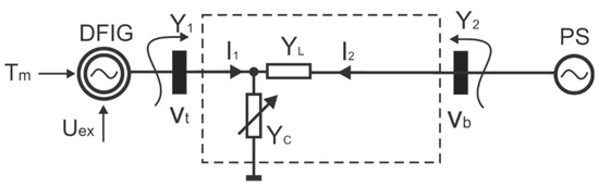
Figure 1.
Induction generator with a local consumer connected to a power grid.
The considered situation is often found in reality, when the generator (connected to a power grid through a long transmission line) has also equipment and devices (that provide certain related functions absolutely necessary for the normal functioning of the power plant) or even some industrial consumers (close to the plant), which are directly supplied from the generator terminals. The connection between the induction generator and the power system, including local electrical consumers connected at generator terminals, can be described by a quadripole (as shown in Figure 1). Based on quadripole theory, the input and output currents are given by the matrix equation [28,35]:
where:
- is line admittance: (: line conductance, : line susceptance).
- is electrical consumer admittance: (: consumer conductance, : consumer susceptance).
The transmission line admittance seen at the generator terminals is:
The transfer admittance between the generator and the power grid is:
Denoting the generator terminal current (see Figure 1) and using (9) and (10), the following relation results:
Therefore, for a rotor angle , the projections on d-q axis of the generator terminal current are:
As shown in Figure 1, both ends of the considered quadripole are inputs. Therefore, two current supply sources, injecting current into quadripole, can be noticed. The terminals of the stator load winding being the generator terminals, the relationship between the stator load currents and (see Equations (1)–(7)) and the projections and of I terminals current on d-q axis (see Equations (12) and (13) describing the current at corresponding quadripole end) is given by the equalities:
Similarly, and are voltage projections of stator load winding on d-q axis (and also projections of generator terminals voltage on d-q axis). Because the terminal voltage () is the controlled output, solving the equations system (12) and (13) to compute the voltage projections, results the following relations:
and, therefore, the generator terminal voltage (effective value) can be calculated as:
In the performed research, instead of the conductance (, ) and susceptances (, ) the line and consumer resistances (, ) were used, respectively the line and consumer reactances (, ) (see Relations (18)–(21)):
Considering a long transmission line with constant parameters for connection to the power system, the line conductance and susceptance are constants (so, also resistance and reactance of the line are constant). For all presented case studies, only the electrical resistance of the consumer is considered variable (simulating an electrical load/unload by connecting/disconnecting consumers at generator terminals), thus, and are also variable. Many other studies regarding the consumer reactance variation were also performed, but are not presented in the paper (the conclusions being the same). Such variations of or are major disturbances that can affect the system output (terminal voltage), as will be presented in the next chapters.
To avoid an algebraic loop error that can occur during the simulation of the designed model, the main idea is to solve the Equations system (1)–(7) by calculating the windings currents (, , , , , ) which are also process state variables. The d-q axis projections of the generator terminals current and ) are described by Equations (12) and (13), allowing their computation. Using the computed current projections, the Relations (15) and (16) allow the determination of voltage projections ( and ) at the generator terminals. Therefore, the value of the generator terminal voltage is calculated based on Relation (17).
Equations (1)–(7) and (12)–(21) (practically, a 7th order nonlinear model) completely describe the behavior of interconnected systems (induction generator, long transmission line, local electrical consumer, and power system). This model ensures good accuracy for process dynamics in various operating regimes (active/reactive power loading/unloading, connecting/disconnecting local consumers, etc.). The model input is the excitation voltage , and the generator terminals voltage is the process output. The disturbances acting on the controlled process are the mechanical torque (active power load) and the electrical consumer resistance , affecting the admittance seen at the generator terminals and allowing simulation of load/unload regimes by connecting or disconnecting local consumers.
An experimental double fed induction machine (a prototype) is considered having the following main parameters (index N denoting rated values): PN = 1.5 KW, UN = 230/400 V, IN = 2.06/3.57 A, n0 = 1500 rpm, cos ϕN = 0.776, sN = 5.79%, p = 2 (number of pair poles), Ld21 = Ld12 = Lq21 = Lq12 = 0.333 H, L1h = 0.318 H, Lq1 = 0.334 H, Lq2 = 0.334 H, Lq1 = 0.331 H, Ld1 = 0.334 H, Ld2 = 0.334 H, Ld3 = 0.334 H, R1 = 16 Ω, R2 = 16 Ω, R3 = 4 Ω, J = 0.00415 kg·m2. The stator windings w1 and w3 are placed in the same stator cuts; the w2 winding is spatially lagged with 90 electrical degrees in relation with the w1 winding.
3. Design of the Minimum Variance Control System
The general structure of the designed minimum variance control system used in all case studies performed in this paper is presented in Figure 2. The wind turbine and the gearbox are only symbolically presented in this figure as elements of a wind energy conversion system. Only the mechanical torque at the generator shaft is taken into account as a process input (its variation, produced by wind gusts, disturbing the system). For the power converter, used as the power actuator of the control system, a simple first-order delay model (a PT1 element with a small time constant, so very fast-acting) was considered and integrated into control system [36,37].
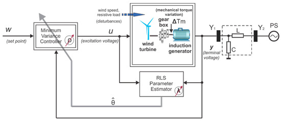
Figure 2.
The minimum variance control system for the induction generator.
The controlled process integrates both wind turbine (subject to external perturbation caused by the wind speed variation) and induction machine connected to a power system and having an additional local consumer at terminals. The following notations were used: : set point, : controller output (excitation voltage), : controlled output (terminal voltage) and : mechanical torque provided by wind turbine through gearbox. Maintaining a constant voltage at the generator terminals is required in the context of connection with the power system [3,32,33].
The 7th order nonlinear model, designed in the previous chapter (describing the entire interconnected system consisting of the induction generator, electrical consumer, transmission line, and power system), is used to simulate the controlled plant in all performed case studies. As was already mentioned, the simplified linear model obtained through linearization around a steady-state point is used only to design the minimum-variance control law [27,28].
An approximation of the process dynamic around a functioning point by an nth order discrete linear equation can accurately enough describe process functional behavior in the considered point vicinity, with the condition to choose a proper model order [2,3,23,24,25,26,27]:
where:
and, for the considered process (induction generator):
- yt: controlled output (terminal voltage) at discrete time t;
- : controller output (excitation voltage);
- : shift operator (with one sampling time, therefore, and so on;
- , : process model parameters (corresponding to polynomials A (q−1) and );
- : model orders taken into account;
The minimization of a classic cost criterion function is used to design the control law [1,2,6].
where : steady state controller output; : set point; ρ: control penalty factor; E{.}: mean operator.
Criterion Function (24) expresses the two goals of the designed control law: minimize the control system’s output variance and minimize the control variance. The importance of the second quadratic term in the criterion function is weighted by a parameter called control penalty factor, commonly set in the range . The higher it is, the more severely the control variance is penalized to the detriment of the controlled output penalization. In theory, if , an optimal control system results by minimizing Criterion Function (24). In practice, such a control system is unfeasible, leading to the process inverse model as a controller. In addition, the control has huge, physically unrealistic levels, and the control system becomes unstable. Therefore, non-zero value must be set for this control penalty factor, leading to a suboptimal control system (the control being limited to physically achievable values) [1,2,3,6,7].
By minimizing the considered Criterion Function (24) and taking into consideration the Linearized Model (22), the control law becomes (25) [2,3]:
Figure 3 systemically described this Control Law (25), highlighting the fact that linearized model is used only for the design phase of the control law (entire calculation algorithm being published by the authors in [2,38]).
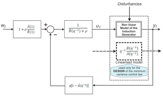
Figure 3.
The minimum variance control law (, —polynomials of estimates).
By using Relation (23) in generalized Control Law (25), the following control law results (26):
where , are estimations of model parameters and as chosen values for analysis.
Using the resulting control laws (Relation (26) particularized for ), a suite of tests were performed to compare the corresponding obtained results. As is already mentioned, the induction generator is integrated into a wind energy conversion system operating under constraints imposed by the connected power system, a local consumer being also connected at generator terminals. In this context, the goal of the control system is to maintain a constant terminal voltage by rejecting external disturbances. These disturbances occur due to variation of the mechanical torque provided by the wind turbine (caused by wind speed variation) or due to variation of consumer resistance (caused by connecting/disconnecting consumers at generator terminals). By analyzing the obtained control law (Relation (26)), one can notice the parameter ρ (control penalty factor) that needs to be set appropriately for tuning the control system. In the cost criterion function, this parameter weights the term that minimizes the control variance. A higher value of ρ imposes a strong penalty of control variance, but at the expense of a good penalty of controlled output variance. Furthermore, the control system stability is strongly dependent on the value of this parameter [2,3,7]. The dynamics of the control law is also influenced by the dynamics of the parameter estimations (online identified by the recursive least squares (RLS) estimator). Although it does not come out explicitly in the control law expression, the initial off-line tuning of the parameter estimator by setting a proper value for the forgetting factor λ can also affect control performances [39].
Based on Relations (22) and (23), a 4th order discrete transfer function can model accurately enough the functionality and dynamic behavior of the induction generator, around an operating point [2],
By substituting from Equation (25) into Equation (27), the control system transfer function can be express as:
Based on the denominator of this discrete transfer function (Relation (28)), the characteristic equation of the control system is:
The system stability can be analyzed assuming non-deviation conditions for the estimates in a steady-state regime [2,3].
By taking into consideration this assumption (Relation (30)), the control system characteristic Equation (29) becomes
Therefore, the control system stability can be analyzed by studying the root placements of the characteristic Equation (31) inside or outside of the unitary radius circle. An analysis of this characteristic equation denotes the fact that the control penalty factor is the main tuning parameter that can affect system stability [2,3]. So, there results in the possibility to ensure the control system stability by an adequate setting of ρ. This can be done only through successive tests, considering different values of ρ. The control system stability will also be proved in the next section by presenting performed robustness tests.
4. Case Studies
Two sets of case studies were analyzed in the paper, each of them considering successively a control law designed based on a linearized process model of 5th, 4th, and respectively, 3rd order. The first set (case A: see Table 1, second column) considers a step variation of mechanical torque (∆Tm) due to wind speed variation. The second set considers, as a disturbance, a step resistive load () by connecting a consumer at generator terminals (case B: see Table 1, third column). For all cases, the study analyzes the control system’s ability to reject the effect of such process disturbance. In the following, each case is presented and analyzed in extenso, highlighting the results and performances provided by each of the three control laws.

Table 1.
Summary of the case studies.
Table 1 summarizes the tested control strategy, analyzing the following control system quality indicators: settling time (the main indicator), overshoot, the time length of the oscillating regime, and the maximum controller output. The last quality indicator is practically the excitation voltage, its analysis being important in the context when one objective of the considered criterion function (Relation (24)) consists in minimizing the control variance to obtain a physically achievable excitation voltage value. In addition, in Table 1 are briefly presented comparative comments on the results obtained for each control law.
In addition to external disturbances (already mentioned), the system is perturbed by a stochastic noise with variance σ2 = 0.01, as a required condition for proper functioning of the parameters estimator (RLS) [2,3,6]. The objective of performed studies is to identify a set of appropriate values for the two parameters required by control system tuning: the control penalty factor ρ (specific to the minimum variance control law), respectively, the forgetting factor λ (specific to the parameter estimator). It is mentioned that several tests were performed considering various values for the set of controller tuning parameters (ρ, λ), but only the case studies that provided the best results are presented in this paper. It should also be mentioned that, for all cases, a settling band was defined (±0.1%) and considered to analyze the control system response (terminal voltage).
4.1. Case A: Mechanical Torque Variation ()
The next tests consider the process perturbed by an external disturbance at time t = 1 s, produced by mechanical torque variation (see Table 1).
4.1.1. Case Study A.1 (5th Order Model)
In this first case study, a minimum variance controller designed based on the 5th order linear model is analyzed (the control law being described by Relation (26) particularized for order n = 5). The best results (see Figure 4a,b and Figure 5a,b) were obtained for the set of parameters λ = 0.995 and ρ = 0.0725.
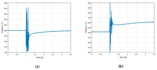
Figure 4.
Mechanical torque variation—5th order model: (a) Terminal voltage (controlled output); (b) Excitation voltage (controller output).
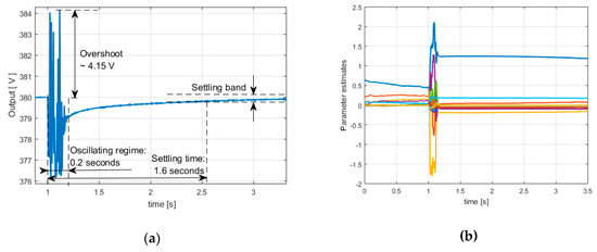
Figure 5.
Mechanical torque variation—5th order model: (a) Terminal voltage—zoom; (b) Parameter estimates.
Figure 5a shows a zoom on the controlled output (terminal voltage). A long settling-time (1.6 s) can be noticed, an overshoot slightly over 4 V, and a short oscillating regime (0.2 s). The controller output (excitation voltage) is presented in Figure 4b, and a good penalization of its variance can be noticed. Therefore, the control is in a range of physically achievable values (maximum value of excitation voltage being 500 V). The parameters estimates (outputs of a considered recursive least square estimator (RLS)) are represented in Figure 5b (under action of a stochastic noise with zero mean and variance σ2 = 0.01) and their evolution is numerically stable.
As a conclusion, in this case, control system performances are acceptable (the settling-time being a little too long).
4.1.2. Case Study A.2 (4th Order Model)
The second case study was performed starting from a 4th order process linear model. The best results (see Figure 6a,b and Figure 7a,b) were obtained for the set of parameters λ = 0.995 and ρ = 0.0001. A significant decrease of settling-time (to 0.27 s) can be seen in Figure 7a. Therefore, this control quality indicator is much better than that of the controller based on 5th order model (and so this low-order controller is faster). In addition, the response overshoot is slightly under 4 V (lower than in previous case) and oscillating regime is slightly longer (0.25 s). A decrease of the control variance can be noticed (Figure 6b, maximum excitation voltage: 475 V), and it can be concluded that the control is in a range of physically achievable values, even under the conditions of a very low control penalty factor (ρ = 0.0001). Figure 7b shows the process parameters estimates. The parameter estimates will not be depicted for the next cases, their evolution being good and they do not affect the conclusions of performed studies. In conclusion, the settling-time (as a main control quality indicator) being much shorter and all other indicators being comparable, the performances of this 4th low-order control law are superior to a controller designed based on a 5th order model.
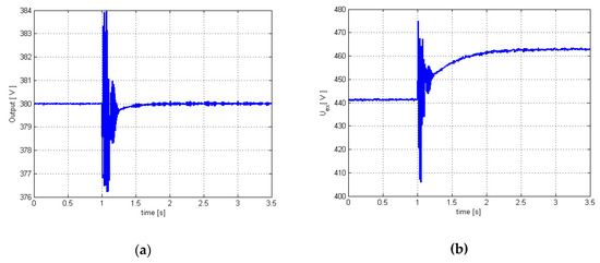
Figure 6.
Mechanical torque variation—4th order model: (a) Terminal voltage (controlled output); (b) Excitation voltage (controller output).
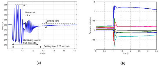
Figure 7.
Mechanical torque variation—4th order model: (a) Terminal voltage—zoom; (b) Parameter estimates.
4.1.3. Case Study A.3 (3rd Order Model)
The third case study was conducted using the 3rd order process linear model to design the minimum variance controller (with tuning parameters λ = 0.99 and ρ = 0.0725, for best results). A comparison between the results of this case (Figure 8a,b) and the ones obtained in previous cases (Figure 4a,b and Figure 6a,b) show much weaker performances of this 3rd order control law. Figure 8a (controlled output) shows a large increase of settling-time (over 2 s), oscillating regime becomes much too long (about 1.7 s), and the overshoot is almost double (over 8 V) compared to previous cases. Furthermore, the excitation voltage (controller output) is much higher (even in the context of a much stronger control penalization), maximum excitation voltage being 680 V (see Figure 8b). This value of control penalty factor is the smallest which still ensures the stability of control system (below this threshold, the system becomes unstable). Any higher value of ρ leads to a degradation of controlled output performance. Overall, performances provided by this low-order control law are poor.
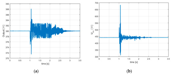
Figure 8.
Mechanical torque variation—3rd order model: (a) Terminal voltage (controlled output); (b) Excitation voltage (controller output).
As a final conclusion of Case A (see Table 1), based on the previous analysis regarding the set of tests performed for the case of a mechanical torque variation, the control law based on the 4th order model provide the best control performances (see also all three responses of control systems depicted overlapped in the same Figure 9).
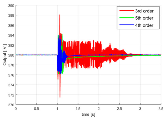
Figure 9.
Terminal voltages—overlapped.
4.2. Case B: Resistive Load ()
This new tests set considers an external disturbance (at time t = 1 s) produced by a resistive load () due to the connection of a new consumer. In all these case studies (see Table 1), for each of the three control law, the same values of the controller parameters (λ and ρ) were used as in previous cases (A).
4.2.1. Case study B.1 (5th Order Model)
The first case study considers a minimum variance controller designed based on the 5th order linear model. The results (obtained for the same tuning parameters λ = 0.995 and ρ = 0.0725, as in Case A) are depicted in Figure 10a,b and Figure 11a–c. As expected for this higher-order controller, the performances are very good (see also Table 1): short settling time (0.1 s, considering the defined settling band ± 0.1%, see first yellow point in Figure 11b), short overshoot (3.4 V, see Figure 10a), short oscillating regime (under 0.1 s, see Figure 11b) and low maximum controller output (443 V, see Figure 10b).
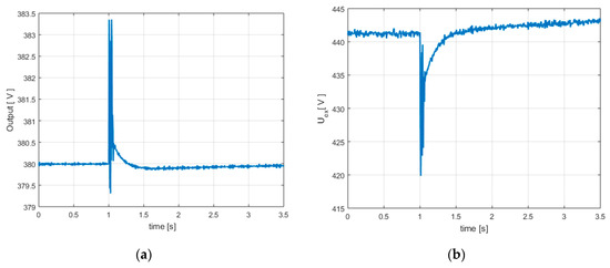
Figure 10.
Resistive load—5th order model: (a) Terminal voltage (controlled output); (b) Excitation voltage (controller output).
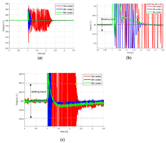
Figure 11.
Terminal voltages—resistive load: (a) Terminal voltages—overlapped; (b) Terminal voltages—zoom 1 (c) Terminal voltages—zoom 2.
4.2.2. Case Study B.2 (4th Order Model)
Taking into consideration a reduced 4th order model of the controlled process, the resulting simplified control law also provides very good performance (Figure 12a,b and Figure 11a–c): short settling time (0.18 s, see second yellow point in Figure 11b), short overshoot (4.2 V, see Figure 12a), short oscillating regime (under 0.2 s, see Figure 11b) and reasonable maximum controller output (460 V, see Figure 12b). Overall, the performances are very close (negligibly weaker) to those provided by the control law from the previous case.
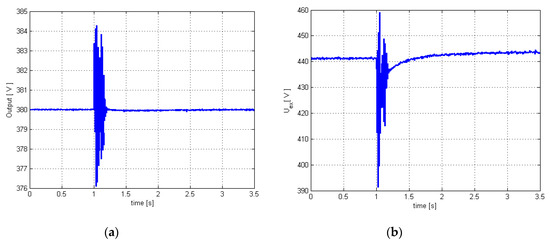
Figure 12.
Resistive load—4th order model: (a) Terminal voltage (controlled output); (b) Excitation voltage (controller output).
4.2.3. Case Study B.3 (3rd Order Model)
Very poor performances can be observed in Figure 13a,b and Figure 11a–c: much longer settling time (1.3 s, see second yellow point in Figure 11c), small overshoot (over 4.5 V), much longer oscillating regime (1.3 s), maximum excitation voltage over 640 V (Figure 13b). Therefore, the control law designed based on 3rd order linear model has much weaker performances being unable to accurately describe the dynamics of the real controlled process, and as a consequence, the controller is basically under-dimensioned (operating in a forced mode with higher voltage excitation values, but with poor performances). These remarks regarding this low-order control law are also valid both for the case of a resistive load (Case B.3) and the case of a mechanical torque variation (Case A.3). It is also noted that other inductive and capacitive load/unload tests have been carried out, but the conclusions are similar and have not been presented in the paper.
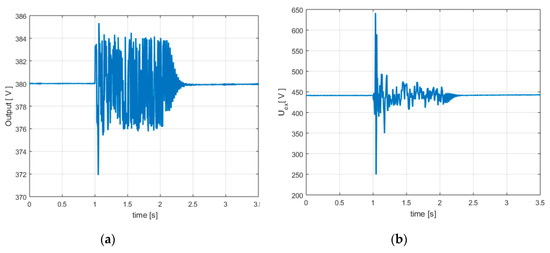
Figure 13.
Resistive load—3rd order model: (a) Terminal voltage (controlled output); (b) Excitation voltage (controller output).
For this selected minimum-variance controller, designed based on 4th order linearized process model, the following test scenarios (Figure 14a,b) analyze the behavior and performances of the controlled process under random disturbances, with focus on stability and robustness analysis of the adaptive control system. For this purpose, two case studies are performed. Similar results (not presented here) were obtained for the controller based on a 5th order linear model, respectively, for the controller based on a 3rd order model, the case for which the performances were very poor. As we already mentioned, in addition to external disturbances, the system is perturbed by a stochastic noise (with zero mean and variance σ2 = 0.01), as a required condition for proper functioning of the parameters estimator (RLS) [2,3,6].
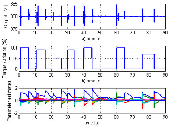
Figure 14.
Robustness test (mechanical torque variations): (a) Controlled output (terminal voltage); (b) Mechanical torque variation (disturbance); (c) Parameters estimates.
The first case study considers a long sequence of random disturbances (see Figure 14b), generated by repeated variations of the mechanical torque (produced by wind gusts). The process output (terminal voltage) shown in Figure 14a demonstrates the control system robustness and stability. In addition, the numerical stability and convergence of the parameters estimator are proven by the result depicted in Figure 14c.
The second case study considers a long sequence of random disturbances (see Figure 15b), generated by repeated variations of the electrical resistance (produced by connecting or disconnecting consumers at generator terminals). The process output (terminal voltage, depicted in Figure 15a) demonstrates the control system robustness and stability. In addition, the result depicted in Figure 14c proves the numerical stability and convergence of the parameters estimator.
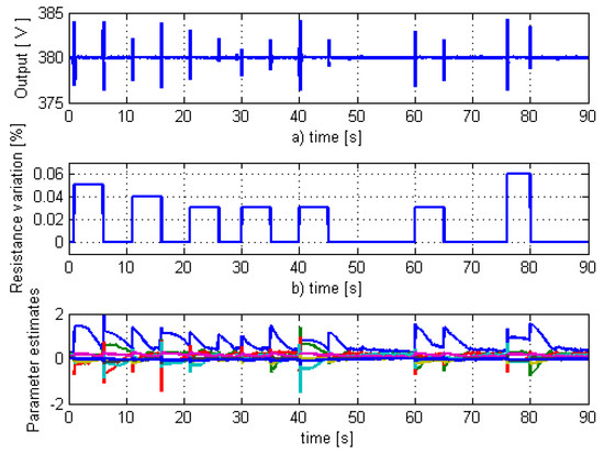
Figure 15.
Robustness test (electrical resistance variations): (a) Controlled output (terminal voltage); (b) Electrical resistance variations (disturbance); (c) Parameters estimates.
Therefore, these test scenarios demonstrate the stability and robustness of the proposed minimum variance control system under a wide range of repetitive random disturbances acting over a long time interval.
By considering the linear model of the control law and the 4th order linear model of the controlled process (as an approximation of the 7th full-order nonlinear model), the frequency response (Bode diagram) and the complex plane characteristic of the control system can be computed around a functioning point. The nonlinear control system stability can be analyzed through several methods. In concordance with the specific of the considered system, several criteria can be used: Nyquist criterion (involving a linearization in the vicinity of an operating point and based on frequency analysis), Lyapunov criterions (there are more methods, and some of them are difficult to implement for high order systems), circle criterion (for nonlinear time-varying parameters systems), Popov criterion (for the autonomous, time-invariant systems), Nash criterion (specific to the games theory), etc. In the following, the Nyquist criterion is used to perform an analysis regarding the control system stability around a functioning point.
Based on frequency response and complex plane characteristic, a study regarding the control system stability is performed in Figure 16 and Figure 17 (Bode diagram, respectively, Nyquist diagram). The Bode diagram presents the magnitude (gain amplitude), respectively, the phase of the control system response in the frequency domain. The Nyquist diagram describes the complex plane characteristic of the control system. Both being representations of the same response (in the frequency domain, respectively, in the complex plan), by using the Nyquist criterion the control system stability can be analyzed (in the vicinity of an operating point).
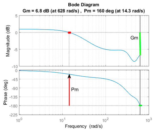
Figure 16.
The frequency domain characteristics of the control system—Bode diagram.
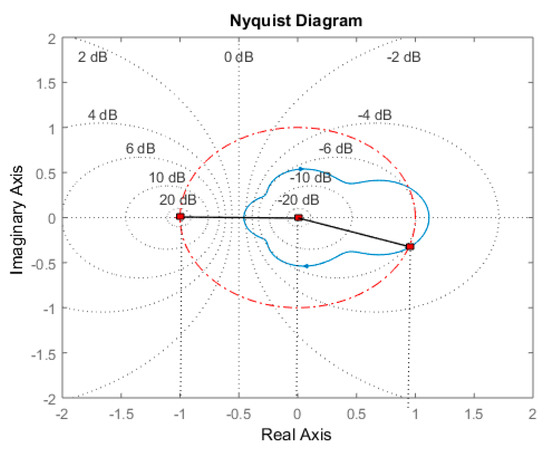
Figure 17.
The complex plane characteristic of the control system—Nyquist diagram.
The reserve phase or phase margin (with red color: Pm = 160 deg. at corresponding crossover-frequency 14.3 rad/s) and the gain margin (with green color: positive Gm = 6.8 db. at corresponding frequency 628 rad/s) can be highlighted (see Figure 16). The control system stability can be analyzed based on the phase margin and gain margin. If the conditions 0 < Pm < 180 deg and Gm > 0 are accomplished, then the analyzed system is stable around the functioning point.
Figure 17 presents the Nyquist diagram of the open-loop system. The Nyquist curve (also known as the sensitivity circle) can also provide information regarding the stability of the closed-loop control system by analyzing the Nyquist diagram of the open-loop transfer function. For this case, the open-loop system is stable (as a series connection of a stable controller and a stable process), it can be noticed that the Nyquist curve does not encircle the critical point (−1,0) (see Figure 17). Moreover, the same phase margin (Pm = 160) can be noticed in the Nyquist diagram (see the phase margin angle Pm with red color in Figure 17). Therefore, the closed-loop system is stable, and so the minimum-variance control system is stable around this operating point.
Additionally, we performed a stability analysis using the indirect Lyapunov method [40]. This method states that: the stability analysis of an equilibrium point (related to the considered functioning point of a nonlinear system) can be done by studying the stability of the corresponding linearized system in the vicinity of this equilibrium point.
For a nonlinear system, the state equation can be written as:
where is the state vector at time , respectively, is the input at time .
Around the equilibrium point , the corresponding linearized system is considered:
According to the reduced Lyapunov criterion, if all the eigenvalues of matrix A have modulus less than 1, then the equilibrium point is also asymptotically stable for the nonlinear system [40].
The following numerical calculations were performed using MATLAB. Considering the operating point of the simulated control system, the linearized model of the closed-loop system can be expressed as a discrete transfer function with the parameter values estimated (by RLS parameters estimator) for the 4th order linear model of the process (see Relations (22) and (23)) and, based on them, with the controller parameters calculated according to the control law (Relation (26)). Thus, the following 7th order discrete transfer function of the control system results.
Based on this discrete transfer function (34), for a state space model (35):
the following matrix is computed:
In addition, by computing the eigenvalues of the state matrix A, the following eigenvector results.
Therefore, the modulus of these eigenvalues of matrix A are
It can be noticed that all the computed eigenvalues of state matrix A (see Relation (38)) have modulus less than 1. Therefore, the equilibrium point is also asymptotically stable for the nonlinear system.
As a general conclusion of the entire conducted research (see Table 1 and the stability/robustness analysis), the best choice from these three possible solutions is the minimum-variance controller based on 4th order linearized process model, which provides simultaneously very good performances and a simplified control-law computation algorithm. Thus, an increased order of the linear model used for the design of the minimum variance control law is not justified. At the same time, a drop below 4th order is no longer satisfactory for the minimum-variance control system.
5. Conclusions
Starting from some simplified linear models of a double-fed induction generator (integrated into a wind energy conversion system), the paper presents a comparative study about performances of a self-tuning minimum variance control structure. The double-fed induction generator is connected to a power system through a long transmission line and also, a local electrical consumer is considered connected at generator terminals. A nonlinear model, describing the complex system resulted by connecting the induction generator, electrical consumer, transmission line, and power system, was designed and implemented to simulate the controlled plant behavior.
As a novelty, a study was conducted with the goal of identifying a minimum order of a linear model (obtained through linearization of the designed nonlinear model around a functioning point) used to synthesize a reduced order minimum variance control law, which, despite its simplicity, is able to provide good control results. Therefore, the question to which the performed studies is answering is: How much can the order of the linearized model of a controlled process be reduced, which is a starting point to design a minimum-variance control law, without affecting the control performance? Considering these issues, such simplified control law could avoid a large amount of computational effort, especially required to estimate a large number of process parameters.
The research proves that a reduced 4th order linear model provides the best control performances, although the induction generator is fully functionally described by a 7th order nonlinear model. Even though the control law based on 5th order linear model (or higher) can provide, for some cases, very close or even slightly better results comparatively to the control law based on 4th order model, simplicity of the latter is a reason for choosing it. Furthermore, although some papers from technical literature show that an induction generator could be functionally described around a functioning point by a 3rd order linearized model, the performed tests showed quite poor performances of a control law based on such low order linear model. As a main conclusion and contribution of the paper, the conducted research reveals the fact that a minimum 4th order linear model of the controlled process (induction generator) should be used to design a simplified minimum variance control system (including both control law and parameters estimator), providing good control performance.
Author Contributions
I.F. and O.P. performed the design of the minimum variance control system. C.V. and I.F. performed the simulations and analyzed the results. I.S. and L.M.-P. contributed to the elaboration of case studies. All the authors have structured and approved the final manuscript.
Funding
This research received no external funding.
Conflicts of Interest
The authors declare no conflict of interest.
References
- Åström, K.J.; Kumarb, P.R. Control: A perspective. Automatica 2014, 50, 3–43. [Google Scholar] [CrossRef]
- Filip, I.; Szeidert, I. Tuning the control penalty factor of a minimum variance adaptive controller. Eur. J. Control 2017, 37, 16–26. [Google Scholar] [CrossRef]
- Filip, I.; Vasar, C.; Szeidert, I.; Prostean, O. Self-tuning strategy for a minimum variance control system of a highly disturbed process. Eur. J. Control 2019, 46, 49–62. [Google Scholar] [CrossRef]
- Bhattarai, R.; Gurung, N.; Kamalasadan, S. Dual Mode Control of a Three-Phase Inverter Using Minimum Variance Adaptive Architecture. IEEE Trans. Ind. Appl. 2018, 54, 3868–3880. [Google Scholar] [CrossRef]
- Yanou, A.; Minami, M.; Matsuno, T. Strong stability system regulating safety for generalized minimum variance control. In Proceedings of the 22nd IEEE International Conference on Emerging Technologies and Factory Automation (ETFA), Limassol, Cyprus, 12–15 September 2017; pp. 1–8. [Google Scholar] [CrossRef]
- Åström, K.J.; Wittenmark, B. Adaptive Control; Addison-Wesley: Reading, MA, USA, 1989. [Google Scholar]
- Filip, I.; Vasar, C. About initial setting of a self-tuning controller. In Proceedings of the 4th International Symposium on Applied Computational Intelligence and Informatics, Timisoara, Romania, 17–18 May 2007; pp. 251–256. [Google Scholar]
- Villani, M. High Performance Electrical Motors for Automotive Applications – Status and Future of Motors with Low Cost Permanent Magnets. In Proceedings of the 8th International Conference on Magnetism and Metallurgy, Dresden, Germany, 12–14 June 2018. [Google Scholar]
- Burwell, M.; Goss, J.; Popescu, M. Performance/Cost Comparison of Induction Motor & Permanent Magnet Motor in a Hybrid Electric Car; Research Report; International Copper Association: Washington, DC, USA, 2013. [Google Scholar]
- Shenglong, Y.; Kianoush, E.; Tyrone, F.; Herbert, H.C.; Wong, K.F. State Estimation of Doubly Fed Induction Generator Wind Turbine in Complex Power Systems. IEEE Trans. Power Syst. 2016, 31, 4935–4944. [Google Scholar] [CrossRef]
- Feifei, B.; Liu, H.; Huang, W.; Xu, H.; Hu, Y. Recent Advances and Developments in Dual Stator-Winding Induction Generator and System. IEEE Trans. Energy Convers. 2018, 33, 1431–1442. [Google Scholar] [CrossRef]
- Maharjan, R.; Kamalasadan, S. A novel online adaptive sensorless identification and control of doubly fed induction generator. In Proceedings of the 2014 IEEE PES General Meeting|Conference & Exposition, National Harbor, MD, USA, 27–31 July 2014. [Google Scholar] [CrossRef]
- Al-Olimat, K.S. Combined direct-indirect adaptive speed control strategy for wind induction generator. In Proceedings of the 45th Southeastern Symposium on System Theory, Waco, TX, USA, 11 March 2013. [Google Scholar] [CrossRef]
- Han, P.; Zhang, Y.; Wang, L.; Zhang, Y.; Lin, Z. Model Reduction of DFIG Wind Turbine System Based on Inner Coupling Analysis. Energies 2018, 11, 3234. [Google Scholar] [CrossRef]
- Widanagama Arachchige, L.N.; Rajapakse, A.D.; Muthumuni, D. Implementation, Comparison and Application of an Average Simulation Model of a Wind Turbine Driven Doubly Fed Induction Generator. Energies 2017, 10, 1726. [Google Scholar] [CrossRef]
- Ekanayake, J.B.; Holdsworthb, L.; Jenkins, N. Comparison of 5th order and 3rd order machine models for doubly fed induction generator (DFIG) wind turbines. Electric Power Syst. Res. 2003, 63, 207–215. [Google Scholar] [CrossRef]
- Wang, C.; Du, Z.; Ni, Y.; Li, C. Simplified Model of Doubly Fed Induction Generator in Normal Operation. In Proceedings of the IEEE International Conference on Power System Technology (POWERCON), Wollongong, Australia, 28 September–1 October 2016. [Google Scholar] [CrossRef]
- Rolan, A.; Lopez, F.C.; Bogarra, S.; Monjo, L.; Pedra, J. Reduced-Order Models of Squirrel-Cage Induction Generators for Fixed-Speed Wind Turbines Under Unbalanced Grid Conditions. IEEE Trans. Energy Convers. 2016, 31, 566–577. [Google Scholar] [CrossRef]
- Chandramohan, K.; Padmanaban, S.; Kalyanasundaram, R.; Bhaskar, M.S.; Mihet-Popa, L. Grid Synchronization of a Seven-Phase Wind Electric Generator Using d-q PLL. Energies 2017, 10, 926. [Google Scholar] [CrossRef]
- Mihet-Popa, L. Wind Turbines Using Induction Generators Connected to the Grid; Politehnica Publishing House: Timisoara, Romania, 2007; ISBN 978-973-625-533-5. [Google Scholar]
- Budisan, N.; Prostean, O.; Robu, N.; Filip, I. Revival by automation of induction generator for distributed power systems, in Romanian academic research. Renew. Energy 2007, 32, 1484–1496. [Google Scholar] [CrossRef]
- Filip, I.; Szeidert, I.; Prostean, O. Mathematical modelling and numerical simulation of the dual winded induction generator’s operating regimes. In Soft Computing Applications; Springer: Cham, Switzerland, 2015; pp. 1161–1170. [Google Scholar]
- Saptarshi, B.; Chandan, C.; Sinha, A. Dual stator induction generator with controllable reactive power capability. In Proceedings of the IEEE 23rd International Symposium on Industrial Electronics (ISIE), Istanbul, Turkey, 1–4 June 2014; pp. 2584–2589. [Google Scholar] [CrossRef]
- Ayala, M.; Gonzalez, O.; Rodas, J.; Gregor, R.; Toledo, S.; Doval-Gandoy, J.; Rivera, M. Modeling and Analysis of Dual Three-Phase Self-Excited Induction Generator for Wind Energy Conversion Systems. In Proceedings of the IEEE Southern Power Electronics Conference (SPEC), Puerto Varas, Chile, 4–7 December 2017. [Google Scholar] [CrossRef]
- Ishchenko, A.; Myrzik, J.M.A.; Kling, W.L. Linearization of dynamic model of squirrel-cage induction generator wind turbine. In Proceedings of the 2007 IEEE Power Engineering Society General Meeting, Tampa, FL, USA, 24–28 June 2007; pp. 1–8. [Google Scholar] [CrossRef]
- Fan, L.; Miao, Z. Modeling and Analysis of Doubly Fed Induction Generator Wind Energy Systems; Academic Press: Cambridge, MA, USA, 2015. [Google Scholar]
- Filip, I.; Szeidert, I.; Prostean, O.; Vasar, C. Analysis through Simulation of a Self-Tuning Control Structure for Dual Winded Induction Generator. In Proceedings of the 2013 IEEE 9th International Conference on Computational Cybernetics (ICCC), Tihany, Hungary, 8–10 July 2013; pp. 147–152. [Google Scholar] [CrossRef]
- Szeidert, I.; Filip, I.; Prostean, O.; Vasar, C. Above Modelling and Adaptive Control of a Double Winded Induction Generator. In Proceedings of the 2018 IEEE 12th International Symposium on Applied Computational Intelligence and Informatics (SACI), Timisoara, Romania, 17–19 May 2018; pp. 97–101. [Google Scholar]
- Feijóo, A.; Cidrás, J.; Carrillo, C. A third order model for the doubly-fed induction machine. Electric Power Syst. Res. 2000, 56, 121–127. [Google Scholar] [CrossRef]
- Abbaszadeh, A.; Lesan, S.; Mortezapour, V. Transient response of doubly fed induction generator under voltage sag using an accurate model. In Proceedings of the 2009 IEEE PES/IAS Conference on Sustainable Alternative Energy (SAE), Valencia, Spain, 28–30 September 2009. [Google Scholar] [CrossRef]
- Poller, M.A. Doubly-Fed Induction Machine Models for Stability Assessment of Wind Farms. In Proceedings of the 2003 IEEE Bologna Power Tech Conference, Bologna, Italy, 23–26 June 2003. [Google Scholar] [CrossRef]
- Beaudoin, J.J.; Wamkeue, R. Practical study of the voltage regulation in a self-excited induction generator with two orthogonal three phase windings stator. In Proceedings of the 2012 25th IEEE Canadian Conference on Electrical and Computer Engineering (CCECE), Montreal, QC, Canada, 29 April–2 May 2012. [Google Scholar] [CrossRef]
- Scherer, L.G.; Tambara, R.V.; Botterón, F.; Camargo, R.F.; Hilton, A.G. Discrete-time adaptive control applied to voltage regulation of induction generator based systems. In Proceedings of the 40th Annual Conference of the IEEE Industrial Electronics Society, Dallas, TX, USA, 29 October–1 November 2014; pp. 4940–4946. [Google Scholar] [CrossRef]
- Xia, D.; Heydt, G.T. Self-Tuning Controller for Generator Excitation Control. IEEE Trans. Power App. Syst. 1983, PAS-102, 1877–1885. [Google Scholar] [CrossRef]
- Filip, I.; Curiac, D.I.; Prostean, O.; Dragan, F. On-line Parameters Estimations of a Synchronous Generator Model. In Proceedings of the 8th International Energy Forum (ENERGEX 2000), Las Vegas, NV, USA, 23–28 July 2000; pp. 245–251. [Google Scholar]
- Kazmierkowski, M.P.; Krishnan, R.; Blaabjerg, F. Control in Power Electronics: Selected Problems; Academic Press: Cambridge, MA, USA, 2002. [Google Scholar]
- Rehtanz, C. Autonomous Systems and Intelligent Agents in Power System Control and Operation; Springer: Heidelberg, Germany, 2003. [Google Scholar]
- Filip, I.; Dragan, F.; Szeidert, I.; Rat, C.L. Design of an extended self-tuning adaptive controller. In Proceedings of the 8th International Workshop on Soft Computing Applications (Sofa 2018), Arad, Romania, 13–15 September 2018. [Google Scholar]
- Wu, D.; Song, J.; Shen, Y. Variable forgetting factor identification algorithm for fault diagnosis of wind turbines. In Proceedings of the Chinese Control and Decision Conference (CCDC), Yinchuan, China, 28–30 May 2016; pp. 1895–1900. [Google Scholar] [CrossRef]
- Haddad, W.M.; Chellaboina, V.S. Nonlinear Dynamical Systems and Control: A Lyapunov-Based Approach; Princeton University Press: Princeton, NJ, USA, 2008. [Google Scholar]
© 2019 by the authors. Licensee MDPI, Basel, Switzerland. This article is an open access article distributed under the terms and conditions of the Creative Commons Attribution (CC BY) license (http://creativecommons.org/licenses/by/4.0/).