Radiation Properties of Conformal Antennas: The Elliptical Source

Abstract

The solution of inverse source problems by numerical procedures requires the investigation of the number of independent pieces of information that can be reconstructed stably. To this end, the mathematical properties of the relevant operators are to be examined in connection with the source shape. The aim of this work is to investigate the effect of the source shape on the eigendecomposition of the radiation operator in a 2D geometry, when the radiated field is observed over a semi-circumference in the far zone. We examine both the behavior of the eigenvalues and the effect of the choice of the representation variables on the point spread function (PSF). In particular, the effect of the choice of the representation variables is considered since operator properties may depend on it. We analyze different source shapes evolving from a line to a semi-ellipse and, finally, to a semi-circumference, in order to understand how the increase of the source aspect ratio affects the results. The main conclusions concern an estimate of the number of degrees of freedom in connection with the source geometry and the fact that the PSF exhibits the same variant behavior along the considered domain, independently of the observation variable. The practical relevance of the result is illustrated by two numerical examples. The first one deals with the conformal array diagnostics for the reliable reconstruction of the excitation of the array elements. The second one concerns the array synthesis problem, and a comparison between the radiating performances of the source geometries is presented.

1. Introduction

Conformal antennas [1] are attracting increasing interest in several applications in radar and mobile communication systems. Array antennas, whose elements are located on a curved surface, may exhibit several advantages not only from the aerodynamical point of view, since they can follow the surface of vessels or aircrafts, but also from the electrical one [2]. In fact, for instance, they can radiate identical focusing patterns within larger angular domains, as required in some surveillance applications [3].

Together with the interest in new array designs, interest is growing in the problems that typically need to be addressed in this area, such as array diagnostics, which deals with determining the presence of possible faulty elements, negatively affecting both gain and sidelobe levels. The array diagnostics problem has been treated in different ways in literature [4,5,6,7,8,9,10]. For instance, in [11], a neural network is exploited to localize a maximum of three faulty elements in a 16-element array, while in [12], a Moore-Penrose pseudoinverse is used to retrieve the current distribution of a planar array of parallel dipoles with faulty elements, and in [13,14], compressed sensing/sparse recovering techniques have been introduced in order to deal with a large amount of data, which is the case of large arrays.

From a more general point of view, diagnostics of such antennas are required to solve an inverse source problem, that of the reconstruction of source currents from the knowledge of the radiated field. Its solution amounts to inverting a linear integral operator. In fact, the radiating source $\mathrm{J}$ and the radiated field $\mathrm{E}$ are linked by the integral radiation operator $ℒ:\mathrm{J}\in \mathcal{X}\to \mathrm{E}\in \mathcal{Y}$, and in order to correctly approach the problem, not only the radiation operator $ℒ$ but also the source and field functional spaces $\mathcal{X}$ and $\mathcal{Y}$ need to be specified.

Moreover, the spectral representation of the relevant operator provides the foundation for an inversion algorithm, which must comply with the stability requirement. In fact, due to the analyticity of the kernel of the integral operator, the number of source current functions that can be correctly reconstructed is finite if uncertainties are available in the data. This number is definite as the number of degrees of freedom (NDF) of the source and depends on both the source and the observation geometries. The NDF represents a figure of merit often used in the literature, and it is involved in different aspects of an information-propagation process. In 1969, di Francia treated the case of an optical system [15], showing that the practical limitation of the NDF was a mathematical phenomenon. Later, the NDF was related to the number of independent channels connecting two volumes that communicate through waves [16,17,18]. Moreover, as discussed in [19,20], the NDF is also linked to the information content of the radiated field. In [21], its link with some symmetry priors about the source space is investigated. As far as concerns the inverse source problem we want to address, the NDF measures the rank deficiency of the operator and hence the level of ill-posedness of the inversion problem [22]. Since the NDF can be valuated as the number of singular values/eigenvalues greater than a threshold depending on the noise [23], we are interested in the singular values decomposition (SVD)/eigendecomposition of the relevant operator in order to provide an estimation of the NDF for a specified kind of source.

Another figure of merit that we shall use is the point spread function (PSF), as the achievable resolution of an inverse scheme can be easily computed by measuring the width of the PSF main lobe [24]. The PSF can be expressed in terms of the singular/eigen functions of the operator $ℒ$ that span the functional space of interest [22].

In a 2D setting, that is, when sources and fields are independent on one Cartesian variable, circumference sources observed over a whole $2\mathsf{\pi }$ observation range in the far zone have been considered in [25,26,27] with both analytical (whenever possible) and numerical approaches. Hereafter, we mean to investigate a different source geometry, that is, a semi-elliptical one, whose far field is observed over a $\mathsf{\pi }$ angle. The first goal of the investigation consists in numerically evaluating the NDF of the source and determining how it is related to its geometry. In addition, the role of the observation variable to be chosen is considered since the results may depend on it.

A second goal is comparing the performances of the operators resulting from the use of different variables within the radiation operator definition. Such a comparison is focused on the numerical analysis of the capability of a stable inversion algorithm to reconstruct point-like sources. To this end, the PSF is considered. It turns out that, when an appropriate variable is adopted, the PSF is nearly independent of the point-like source position for all the examined geometries.

The paper is organized as follows. Section 2 introduces the model equations, and in Section 3, the results about the NDF and PSFs for different source geometries are presented and discussed. A criterion to predict the NDF from the source geometry is proposed and verified. Regarding the PSFs, when the arc length is adopted as an observation variable, they are nearly independent of the source position. A discussion of these results is provided in Section 4. Two antenna applications are shown in Section 5, concerned with array antenna diagnostics and with pattern synthesis problems. Finally, conclusions follow in Section 6.

2. Problem Formulation and Method Description

The source is embedded in a homogeneous medium with dielectric permittivity ${\mathsf{\epsilon }}_0$ and magnetic permeability ${\mathsf{\mu }}_0$ (vacuum). Invariance along the $\mathrm{y}$-axes is assumed, so that the problem formulation is scalar and the surface current sources of interest $\mathrm{J}\left(\underset{\_}{\mathrm{r}}\right)$ are supported over curves belonging to the $\mathrm{x}-\mathrm{z}$ plane.

A point deserving attention concerns the comparison of the results obtained by employing different coordinate systems to represent the source, i.e., Cartesian, polar, arc length coordinates, and the radiated field (i.e., the observation angle and its sine). Therefore, for a semi-elliptic source, the angular variable $\mathsf{\varphi }$ spans between $–\mathsf{\pi }/2$ and $\mathsf{\pi }/2$, while the cartesian variables $\mathrm{x}$ and $\mathrm{z}$ span between $–{\mathrm{a}}_{\mathrm{x}}$ and ${\mathrm{a}}_{\mathrm{x}}$ and between $0$ and ${\mathrm{a}}_{\mathrm{z}}$, respectively. The radiated field, instead, is collected in the far zone on a semi-circumference. When the radiated far field is observed versus the angular variable $\mathsf{\theta }$, the radiation operator, connecting the source current to the far field, normalized to an unessential factor, reads as

$$\mathrm{E}\left(\mathsf{\theta }\right)={{\displaystyle \int }}_{-\mathsf{\pi }/2}^{\mathsf{\pi }/2}\mathrm{J}\left(\mathsf{\gamma }\left(\mathsf{\varphi }\right)\right){\mathrm{e}}^{\mathrm{j}\mathsf{\beta }\left(\mathrm{x}\left(\mathsf{\varphi }\right)\sin \mathsf{\theta }+\mathrm{z}\left(\mathsf{\varphi }\right)\cos \mathsf{\theta }\right)}||{\mathsf{\gamma }}^{\prime }\left(\mathsf{\varphi }\right)||\mathrm{d}\mathsf{\varphi }={ℒ}_{\mathsf{\theta }}\left(\mathrm{J}\right),$$

(1)

where $\mathsf{\gamma }\left(\mathsf{\varphi }\right)=\left(\mathrm{x}\left(\mathsf{\varphi }\right),\mathrm{z}\left(\mathsf{\varphi }\right)\right)$ is a bijective parametrization of the curve over which the integration is performed, and $||{\mathsf{\gamma }}^{\prime }\left(\mathsf{\varphi }\right)||=\sqrt{{\mathrm{x}}^{\prime }{\left(\mathsf{\varphi }\right)}^2+{\mathrm{z}}^{\prime }{\left(\mathsf{\varphi }\right)}^2}$.

When the radiated field is observed versus the variable $\mathrm{u}=\sin \mathsf{\theta }$, it reads as

$$\mathrm{E}\left(\mathrm{u}\right)={\mathrm{a}}_{\mathrm{x}}{{\displaystyle \int }}_{-1}^1\mathrm{J}\left(\mathsf{\gamma }\left(\mathsf{\xi }\right)\right){\mathrm{e}}^{\mathrm{j}\mathsf{\beta }\left({\mathsf{\xi }\mathrm{a}}_{\mathrm{x}}\mathrm{u}+\mathrm{z}\left({\mathsf{\xi }\mathrm{a}}_{\mathrm{x}}\right)\sqrt{1-{\mathrm{u}}^2}\right)}{\mathsf{\gamma }}^{\prime }\left(\mathsf{\xi }\right) \mathrm{d}\mathsf{\xi }={ℒ}_{\mathrm{u}}\left(\mathrm{J}\right),$$

(2)

where $\mathsf{\xi }=\mathrm{x}/{\mathrm{a}}_{\mathrm{x}}$ is the normalized source domain variable, and the curve parameterization is defined as $\mathsf{\gamma }\left(\mathsf{\xi }\right)=\left(\mathsf{\xi },\mathrm{z}\left(\mathsf{\xi }\right)\right)$. In this paper, Equations (1) and (2) are of interest and allow us to define a radiation operator for both the proposed couples of variables, that is,

$${ℒ}_{\mathsf{\theta }}:\mathrm{J}\in {\mathrm{L}}_{\left[-\mathsf{\pi }/2,\mathsf{\pi }/2\right]}^2\to \mathrm{E}\in {\mathrm{L}}_{\left[-\mathsf{\pi }/2,\mathsf{\pi }/2\right]}^2,$$

(3)

and

$${ℒ}_{\mathrm{u}}:\mathrm{J}\in {\mathrm{L}}_{\left[-1,1\right]}^2\to \mathrm{E}\in {\mathrm{L}}_{\left[-1,1\right]}^2,$$

(4)

where $\mathrm{J}$ and $\mathrm{E}$ are assumed to belong to the set of square integrable functions ${\mathrm{L}}_{[·]}^2$ supported over the interval specified by the subscript. Since the operators ${ℒ}_{\mathsf{\theta }}$ and ${ℒ}_{\mathrm{u}}$ are compact, we can compute their eigensystem, that is, the eigenfunctions set $\left\{{\mathrm{v}}_{\mathrm{n}}\right\}$, and the eigenvalues set $\left\{{\mathsf{\lambda }}_{\mathrm{n}}\right\}$.

We specify Equations (1) and (2) for each analyzed source shape, and regarding the NDF, we observe the behavior of the eigenvalues as, for a fixed value of ${\mathrm{a}}_{\mathrm{x}}$, the source extension along $\mathrm{z}$ increases, starting from a linear source (${\mathrm{a}}_{\mathrm{z}}=0$, Section 3.1) to a semi-circumference (${\mathrm{a}}_{\mathrm{z}}={\mathrm{a}}_{\mathrm{x}}$, Section 3.2), through to a semi-elliptic one (Section 3.3). The eigendecomposition cannot always be computed in a closed form, and therefore, we resort to numeric computation when necessary. To this end, the source and the observation domains are discretized with a sufficiently dense number of points. The MATLAB $\mathrm{svd}(\cdot )$ procedure provides a good approximation of the eigendecomposition of the operator with an overall computational effort that scales as the third power of the number of discretization points.

In addition, in order to understand how the source geometry and the limited observation domain may impact the resolution, a PSF analysis is performed by using and comparing the results of the two different sets of variables introduced above. We consider the following PSF expression

$$\mathrm{PSF}\left(\mathsf{\tau },{\mathsf{\tau }}_0\right)={\displaystyle \sum }_{\mathrm{i}=1}^{\mathrm{NDF}}{\mathrm{v}}_{\mathrm{i}}\left(\mathsf{\tau }\right){\mathrm{v}}_{\mathrm{i}}^{*}\left({\mathsf{\tau }}_0\right),$$

(5)

where the $\mathsf{\tau }$ observation variable may refer to either $\mathsf{\xi }$ or $\mathsf{\varphi },$ $\mathrm{and}$ the subscript $0$ concerns the location of the point-like source.

We can see from (5) that since the choice of variables will affect the eigenfunctions, the PSF behavior is affected as well. As for the resolution, it is instead related to the width of the main lobe of the PSF function. The interest in the PSF can be accounted for in order to appreciate the ultimate capability of the inversion scheme to distinguish between two close point sources.

3. Analysis of Some Source Geometries

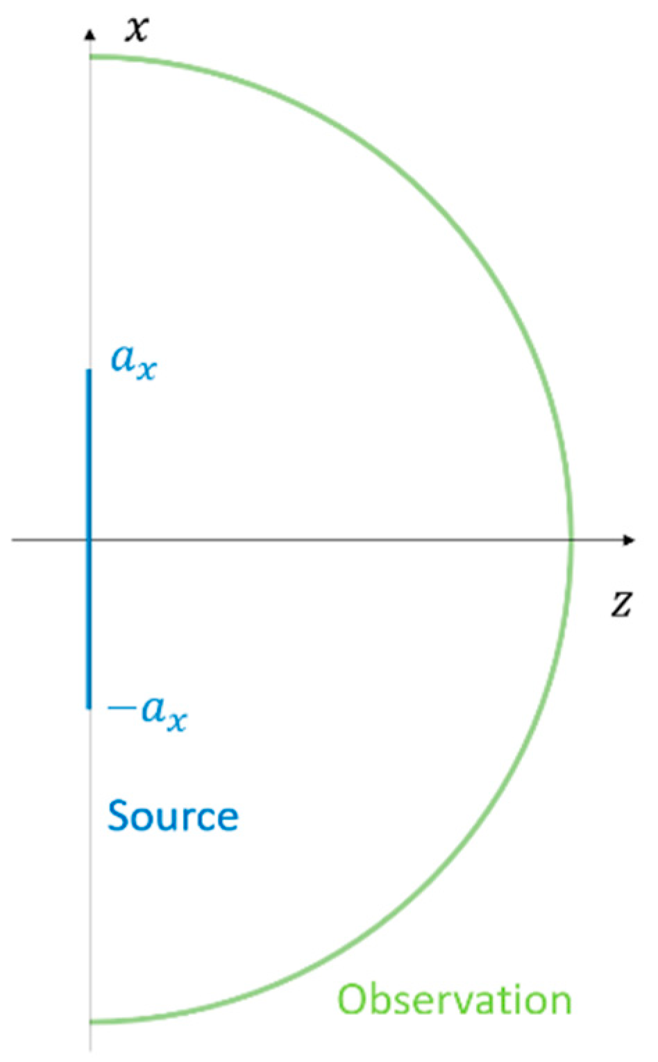
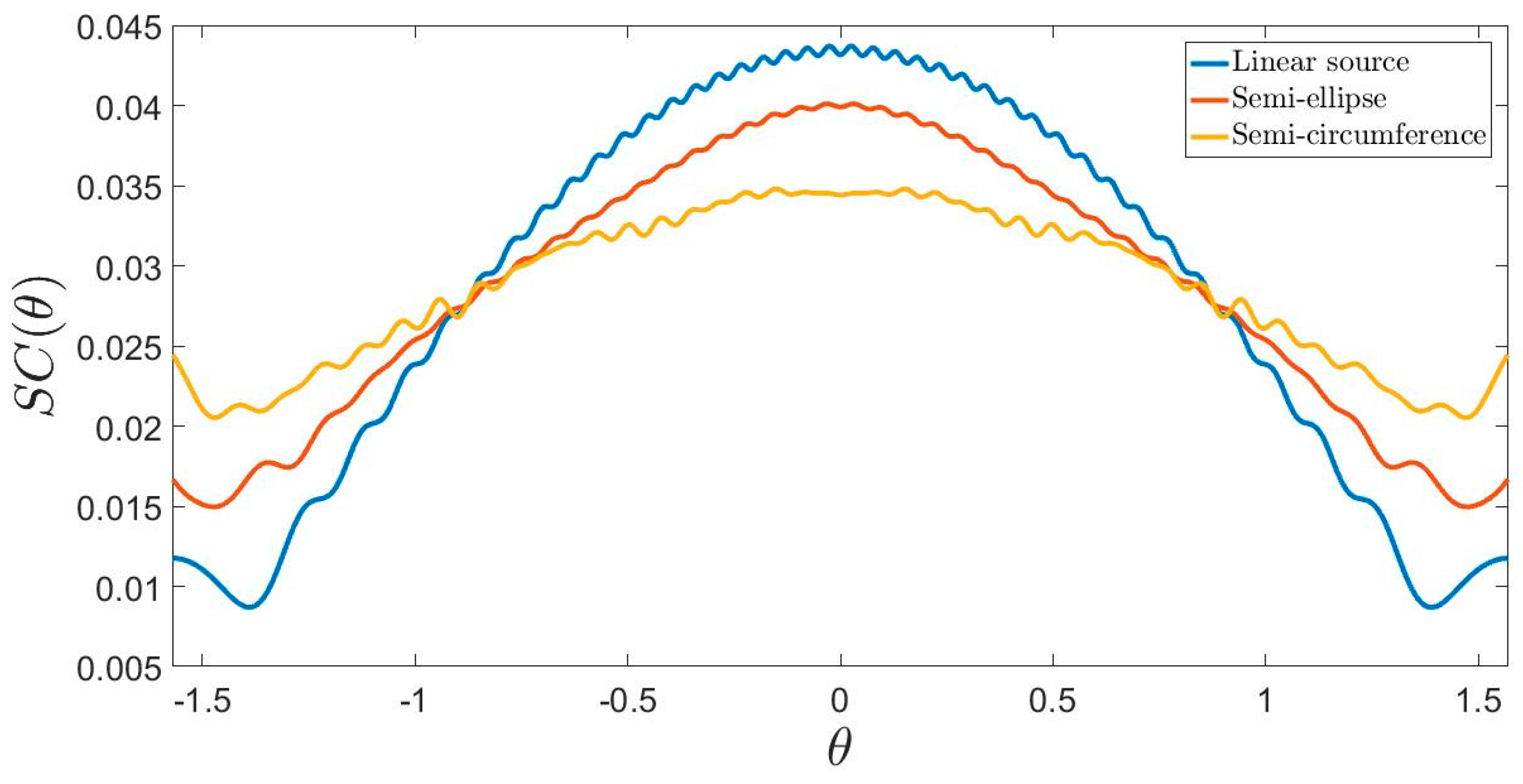
This section may be divided by subheadings. It is meant to provide a concise and precise description of the numerical results about NDFs and PSFs, their interpretation, as well as the conclusions that can be drawn. Results already known in the literature for the linear and semi-circumference sources are recalled in Section 3.1 and Section 3.2, respectively, while in Section 3.3 they are compared with the ones obtained for a generic semi-elliptic source.

3.1. Linear Source

For a $2{\mathrm{a}}_{\mathrm{x}}$ long linear source aligned along the x axis (see Figure 1), Equations (1) and (2) become

$$\mathrm{E}\left(\mathsf{\theta }\right)={\mathrm{a}}_{\mathrm{x}}{{\displaystyle \int }}_{-1}^1\mathrm{J}\left(\mathsf{\xi }\right){\mathrm{e}}^{{\mathrm{j}\mathsf{\beta }\mathsf{\xi }\mathrm{a}}_{\mathrm{x}}\sin \mathsf{\theta }} \mathrm{d}\mathsf{\xi }={\widehat{ℒ}}_{\mathsf{\theta }}\left(\mathrm{J}\right),$$

(6)

and

$$\mathrm{E}\left(\mathrm{u}\right)={\mathrm{a}}_{\mathrm{x}}{{\displaystyle \int }}_{-1}^1\mathrm{J}\left(\mathsf{\xi }\right){\mathrm{e}}^{{\mathrm{j}\mathsf{\beta }\mathsf{\xi }\mathrm{a}}_{\mathrm{x}}\mathrm{u}} \mathrm{d}\mathsf{\xi }={ℒ}_{\mathrm{u}}\left(\mathrm{J}\right),$$

(7)

since for a linear source to introduce an angular variable $\mathsf{\varphi }$ has no meaning. This leads to an operator (6), slightly different from (3), where the source domain spans the interval $\left[-1,1\right],$ different from the observation domain $\left[-\mathsf{\pi }/2,\mathsf{\pi }/2\right]$. In this case the SVD [5] of (6) should be numerically computed.

The eigendecomposition of (7), instead, is known in terms of prolate spheroidal wave functions [28]. A relevant result is that the eigenvalues are almost constant for $\mathrm{n}<\left[\frac{4{\mathrm{a}}_{\mathrm{x}}}{\mathsf{\lambda }}\right]$, where $\mathsf{\lambda }$ is the wavelength, and $[·]$ stands for the nearest integer; after this index they abruptly decay [29]. Moreover, although the singular values/eigenvalues are not the same for operators (6) and (7), the NDF is the same for both cases and the only difference is in the shape of their behavior [27].

For the PSF analysis, as mentioned above, in this case we focus only on the variables $\mathsf{\xi }$. In particular, the property of space invariance of (5) particularized to the $\mathsf{\xi }$ domain is connected to the convolutional form of the kernel of the operators ${ℒ}_{\mathrm{u}}^{†}{ℒ}_{\mathrm{u}}$ and ${\widehat{ℒ}}_{\mathsf{\theta }}^{†}{\widehat{ℒ}}_{\mathsf{\theta }}$, where $†$ stands for the adjoint of the relevant operator. In our configuration, this property holds as the operators ${ℒ}_{\mathrm{u}}^{†}{ℒ}_{\mathrm{u}}$ and ${\widehat{ℒ}}_{\mathsf{\theta }}^{†}{\widehat{ℒ}}_{\mathsf{\theta }}$ can be expressed by convolutional ones as follows:

$$({ℒ}_{\mathrm{u}}^{†}{ℒ}_{\mathrm{u}}\mathrm{f})({\mathsf{\xi }}^{\prime })=\mathsf{\lambda }{{\displaystyle \int }}_{-1}^1\frac{\sin ({\mathsf{\beta }\mathrm{a}}_{\mathrm{x}}(\mathsf{\xi }-{\mathsf{\xi }}^{\prime }))}{\mathsf{\pi }(\mathsf{\xi }-{\mathsf{\xi }}^{\prime })}\mathrm{f}(\mathsf{\xi })\hspace{0.17em}\mathrm{d}\mathsf{\xi },$$

(8)

$$({\widehat{ℒ}}_{\mathsf{\theta }}^{†}{\widehat{ℒ}}_{\mathsf{\theta }}\mathrm{f})({\mathsf{\xi }}^{\prime })={\mathsf{\pi }\mathrm{a}}_{\mathrm{x}}{{\displaystyle \int }}_{-1}^1{\mathrm{J}}_0({\mathsf{\beta }\mathrm{a}}_{\mathrm{x}}(\mathsf{\xi }-{\mathsf{\xi }}^{\prime }))\mathrm{f}(\mathsf{\xi })\hspace{0.17em}\mathrm{d}\mathsf{\xi }.$$

(9)

The expected space-invariance is well verified by the numeric simulation in Figure 2.

Let us now consider the observation domain. In this case, the only noteworthy PSF is the one related to operator (6) since for operator (7), we would find a PSF behavior analogous to that shown for the source domain.

In particular, the properties of the $\mathrm{PSF}$ in the $\mathsf{\theta }$ domain are related to the kernel of ${\widehat{ℒ}}_{\mathsf{\theta }}{\widehat{ℒ}}_{\mathsf{\theta }}^{†}$, which can be written as follows

$$({\widehat{ℒ}}_{\mathsf{\theta }}{\widehat{ℒ}}_{\mathsf{\theta }}^{†}\mathrm{f})({\mathsf{\theta }}^{\prime })=\mathsf{\lambda }{{\displaystyle \int }}_{-\mathsf{\pi }/2}^{\mathsf{\pi }/2}\frac{\sin \left({\mathsf{\beta }\mathrm{a}}_{\mathrm{x}}\left(\sin {\mathsf{\theta }}^{\prime }-\sin \mathsf{\theta }\right)\right)}{\mathsf{\pi }\left(\sin {\mathsf{\theta }}^{\prime }-\sin \mathsf{\theta }\right)}\mathrm{f}\left(\mathsf{\theta }\right)\hspace{0.17em}\mathrm{d}\mathsf{\theta }.$$

(10)

Since the kernel of the integral operator (10) is no longer convolutional, we can deduce that the PSF for the $\mathsf{\theta }$ observation is angularly variant. A numerical evidence of this consideration is given in Figure 3. Thus, observing the radiated field by the $\mathrm{u}$ variable produces a spatially invariant PSF, while observing it by the $\mathsf{\theta }$ variable produces an angularly variant PSF.

3.2. Semi-Circumference Source

When the source is a semi-circumference (Figure 4), operators (1) and (2) are recast as

$$\mathrm{E}\left(\mathsf{\theta }\right)={\mathrm{a}}_{\mathrm{x}}\underset{-\mathsf{\pi }/2}{\overset{\mathsf{\pi }/2}{{\displaystyle \int }}}\mathrm{J}\left(\mathsf{\varphi }\right){\mathrm{e}}^{{\mathrm{j}\mathsf{\beta }\mathrm{a}}_{\mathrm{x}}\cos \left(\mathsf{\theta }-\mathsf{\varphi }\right)}\mathrm{d}\mathsf{\varphi }={ℒ}_{\mathsf{\theta }}\left(\mathrm{J}\right),$$

(11)

and

$$\mathrm{E}\left(\mathrm{u}\right)={\mathrm{a}}_{\mathrm{x}}\underset{-1}{\overset{1}{{\displaystyle \int }}}\mathrm{J}\left(\mathrm{x}\right){\mathrm{e}}^{{\mathrm{j}\mathsf{\beta }\mathrm{a}}_{\mathrm{x}}\left(\mathsf{\xi }\mathrm{u}+\sqrt{1-{\mathsf{\xi }}^2}\sqrt{1-{\mathrm{u}}^2}\right)}\sqrt{1+\frac{{\mathsf{\xi }}^2}{1-{\mathsf{\xi }}^2}}\mathrm{d}\mathsf{\xi }={ℒ}_{\mathrm{u}}\left(\mathrm{J}\right).$$

(12)

For this case, an upper bound to the NDF is provided by [27] as

$$\mathrm{N}\approx \left[\mathsf{\beta }\mathrm{a}\right].$$

(13)

As for a linear source, the NDF is found to be almost the same for both the operators defined in (11) and (12). A numerical verification is reported in Figure 5, where it is quite evident that for both the operators, the eigenvalue steps occur for pretty the same indices and the only difference is in a shaping of the curves. Moreover, the step occurs approximately for an index equal to (13).

It can be expected that the PSF is narrower towards the end points of the domain when we use the variable $\mathsf{\xi }$ instead of the variable $\mathsf{\varphi }$. In fact, the $\mathsf{\xi }$ variable is not linearly linked to $\mathsf{\varphi },$ and this implies that a small increment in the $\mathsf{\xi }$ variable corresponds to a larger one in the $\mathsf{\varphi }$ variable, especially at the end points. From Figure 6, it is evident that the PSFs are both space-variant.

A more uniform comparison for the PSF main lobe widths can be set up by resorting to a different representation variable. To this end, we introduce the arc length $\mathrm{s}$. For the case of a semi-circumference arc, the arc length is simply given by

$$\mathrm{s}\left(\mathsf{\varphi }\right)=\mathsf{\varphi }{\mathrm{a}}_{\mathrm{x}}.$$

(14)

In Figure 7, the overlapped PSFs plotted with respect to the arc length show that the results appear more space-invariant than the previous case.

In particular, while for the operator ${ℒ}_{\mathsf{\theta }}$ there is no difference as the arc length is proportional to the variable $\mathsf{\varphi }$, for the operator ${ℒ}_{\mathrm{u}},$ the percentage variation of the main lobe width between the largest and the smallest PSF displayed in Figure 6 is about 48%, against a value of 26% for the case displayed in Figure 7 (right panel). Since a smaller percentage corresponds to a smaller variation in the resolution, we can state that the use of the arc length variable results in a more uniform behavior. It is apparent that although a perfect spatial invariance of the PSFs is not assured, their width is very similar for all point source positions.

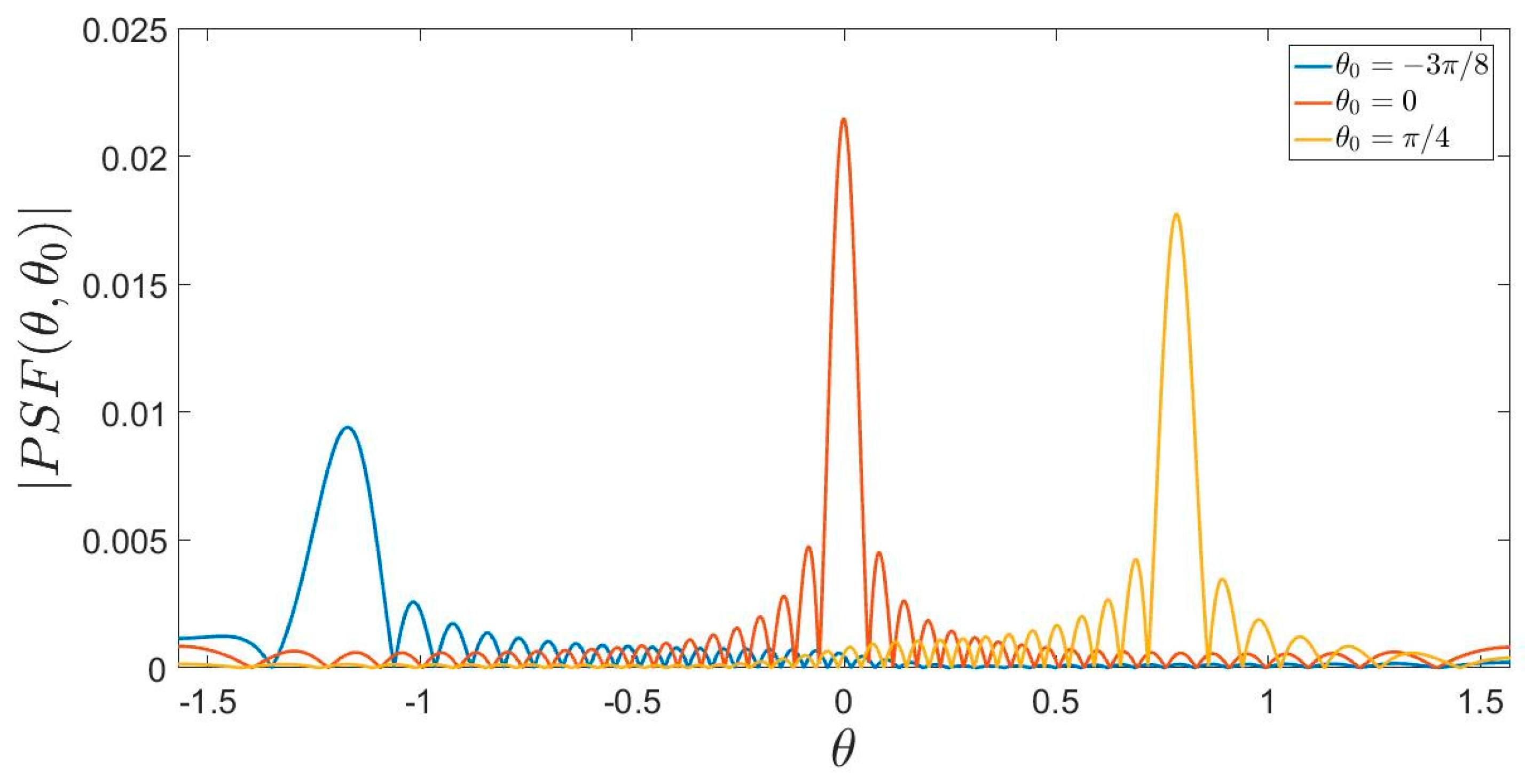
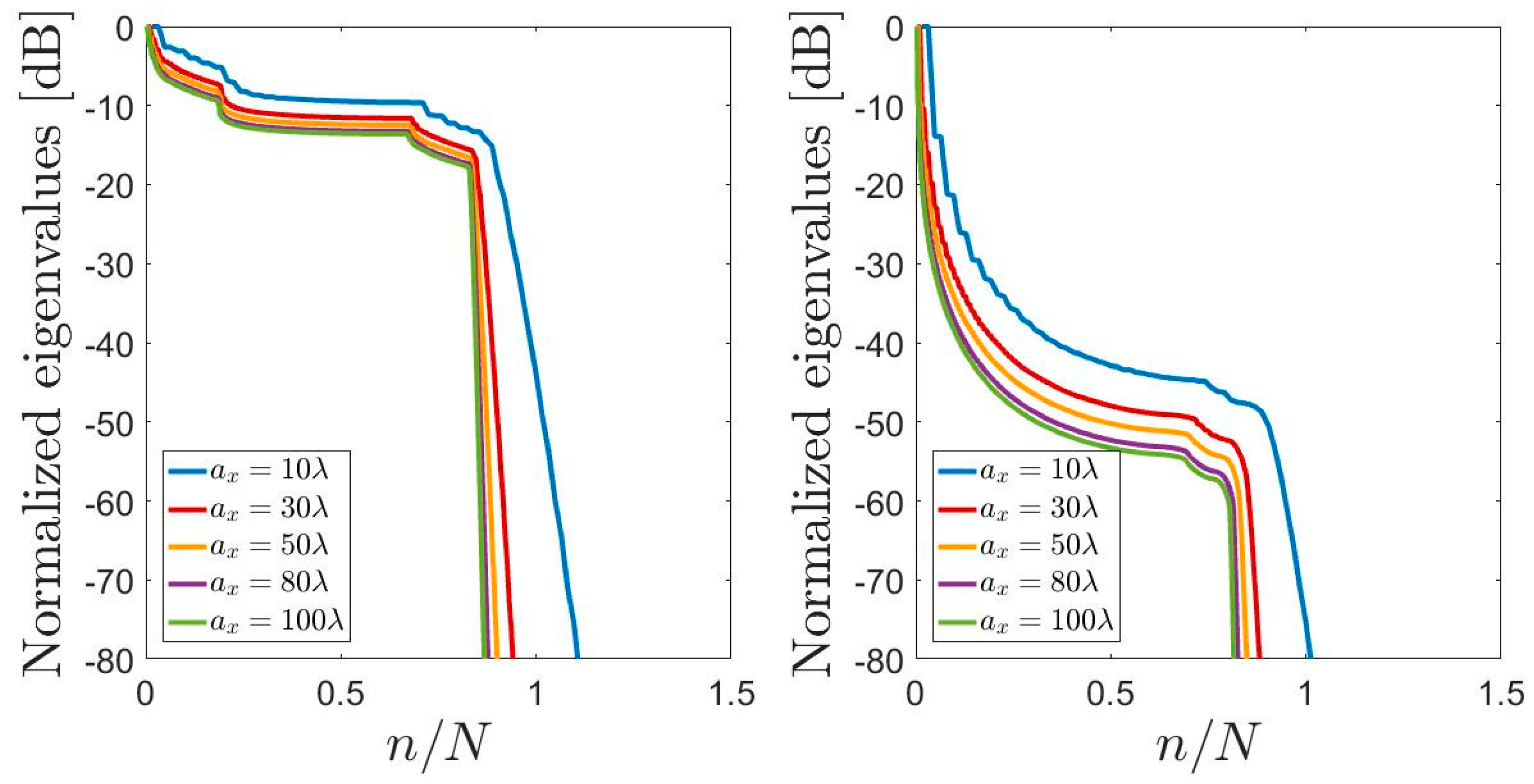
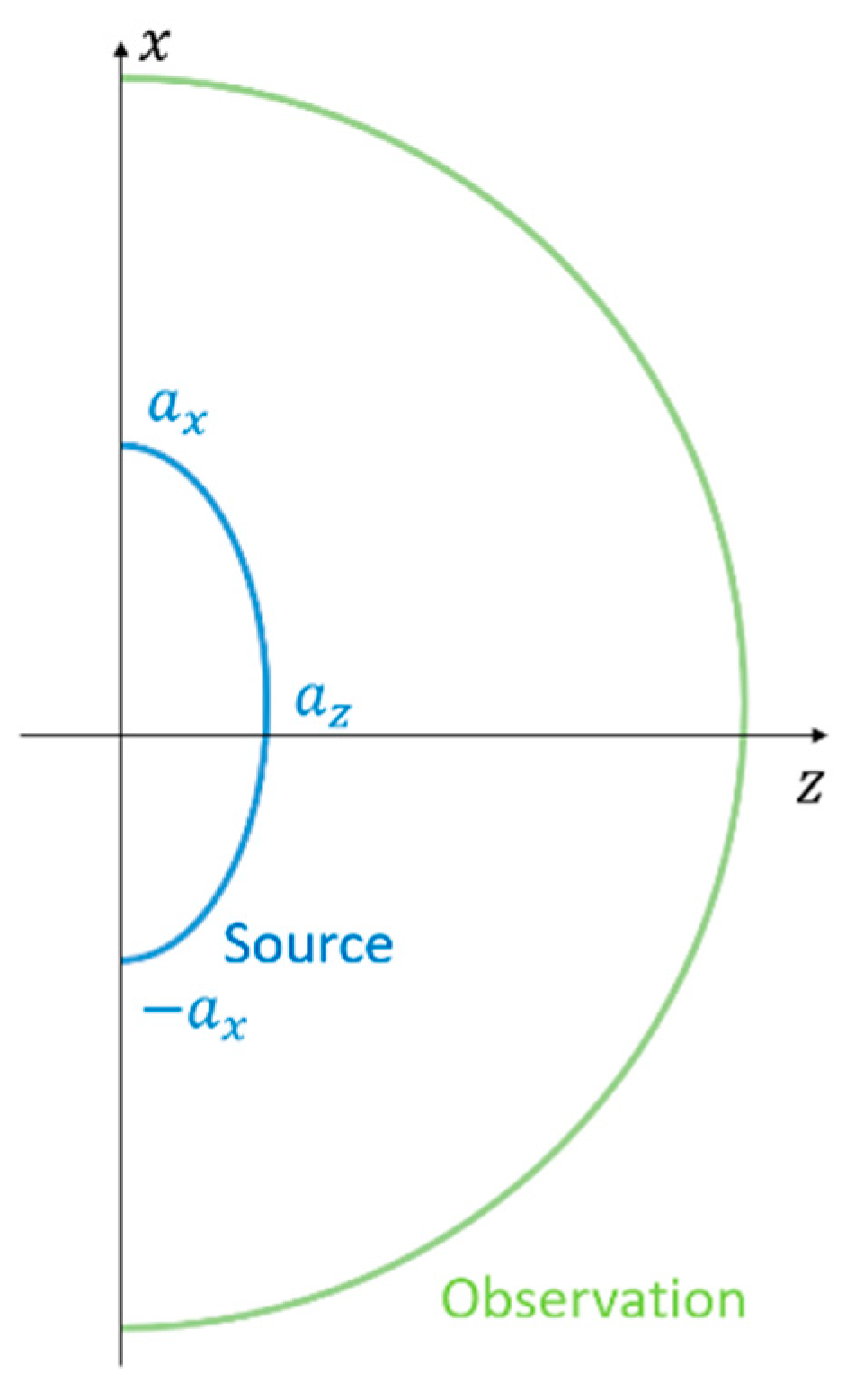
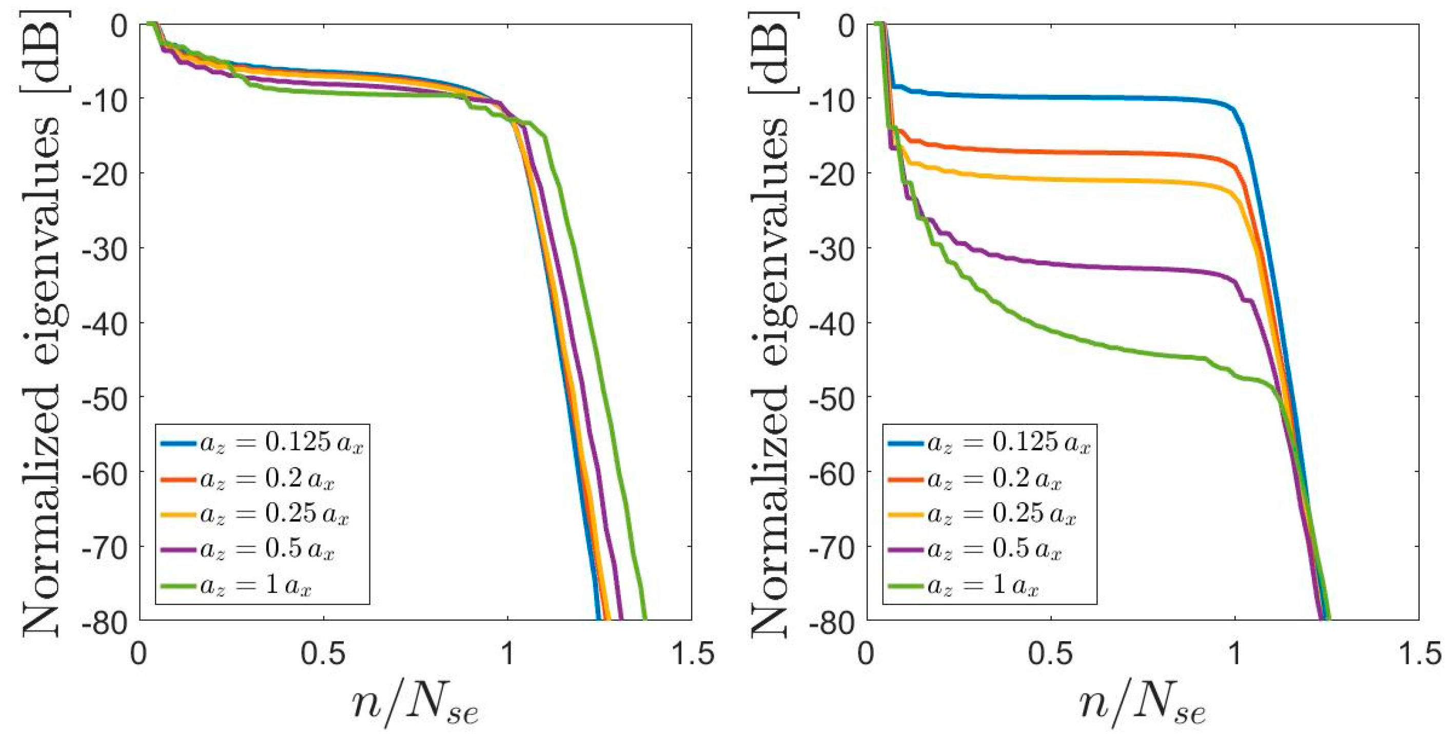
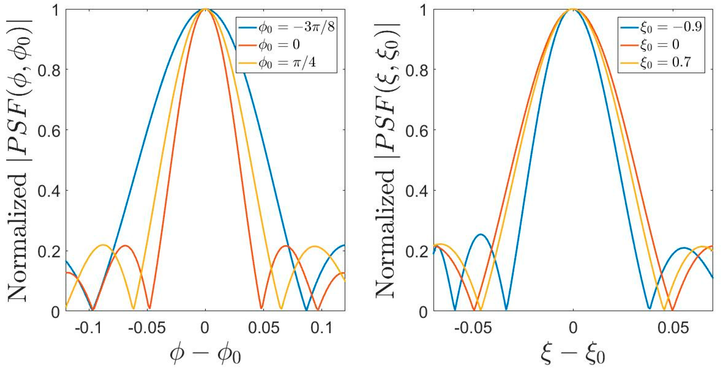
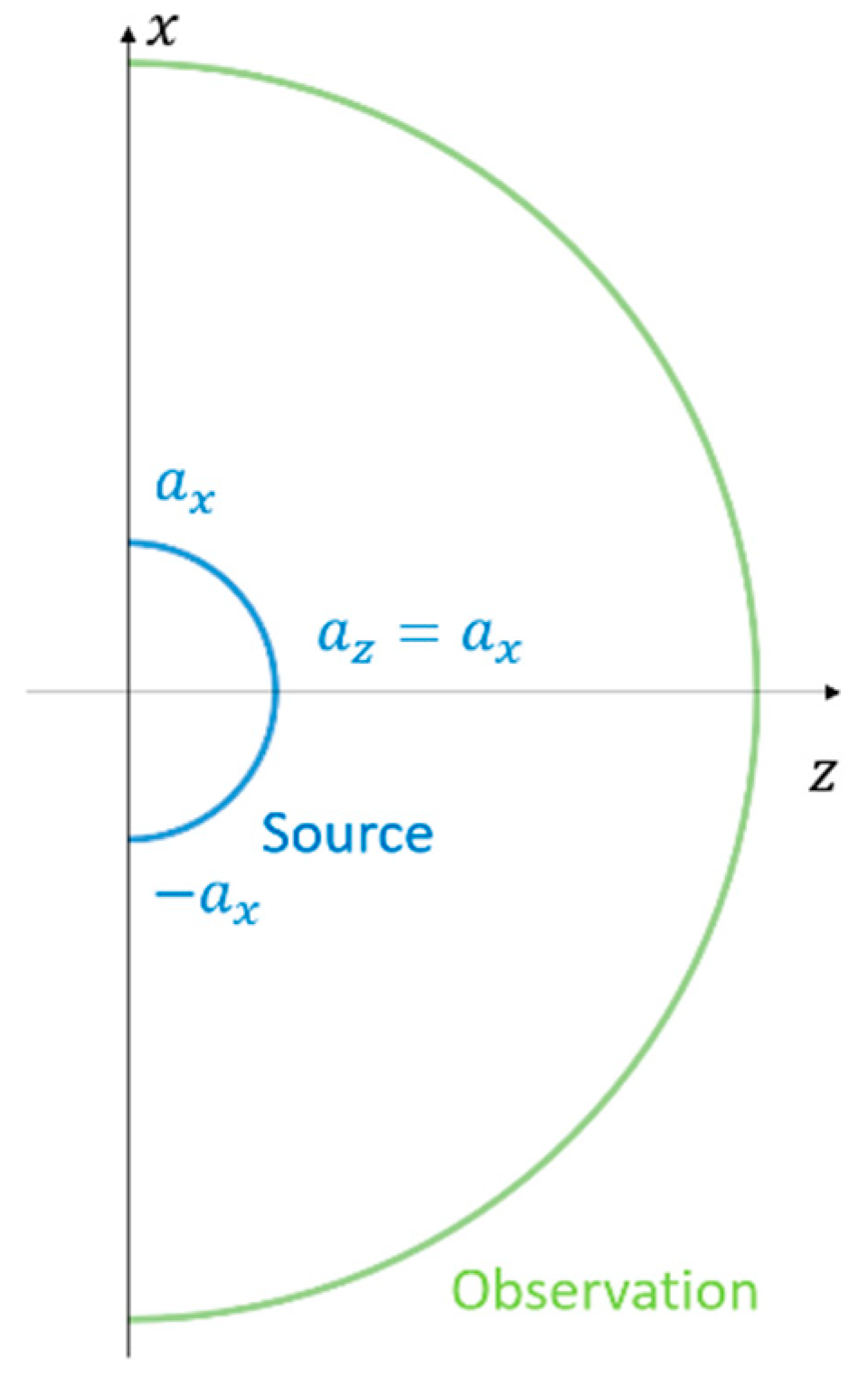
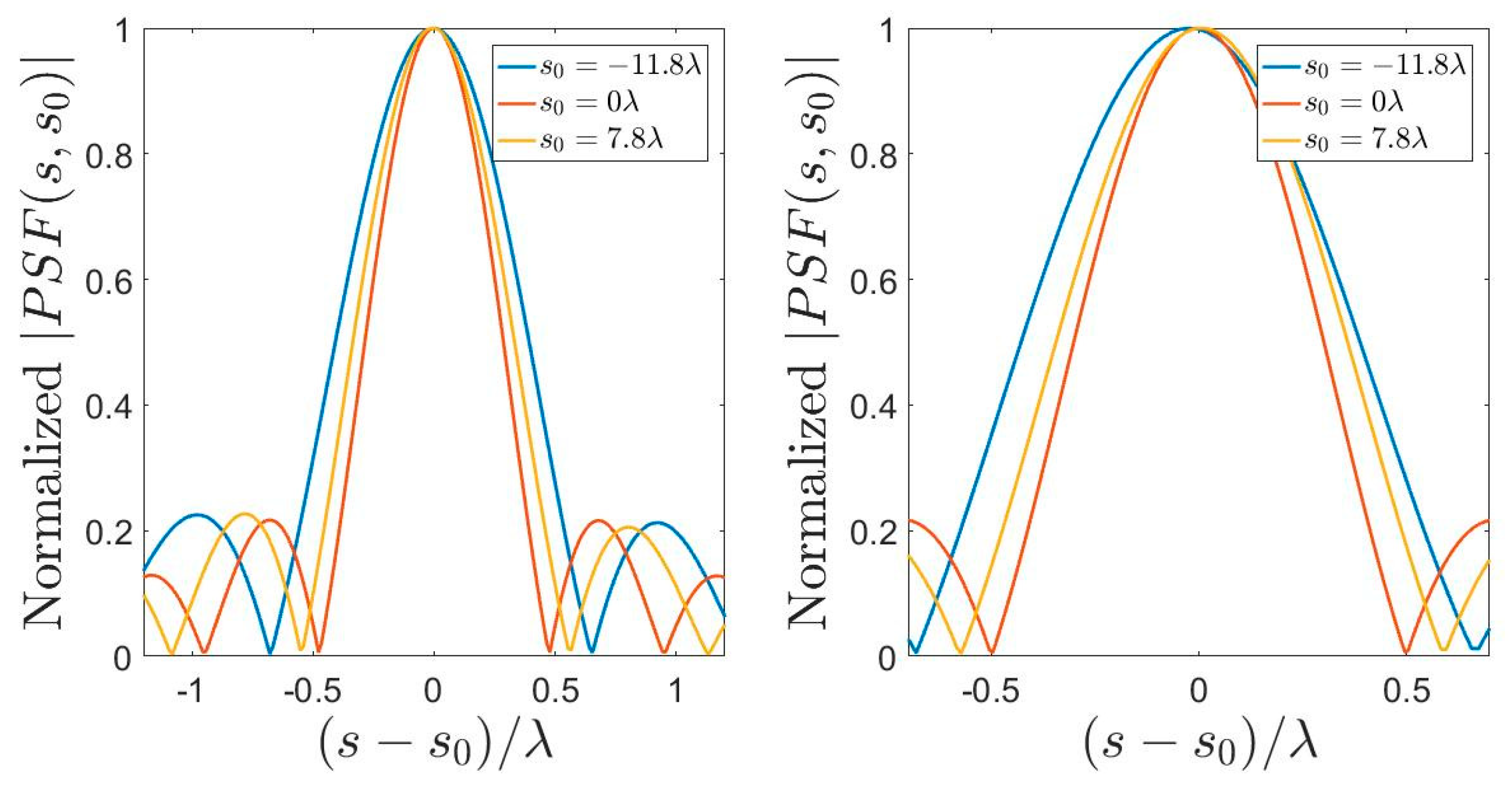
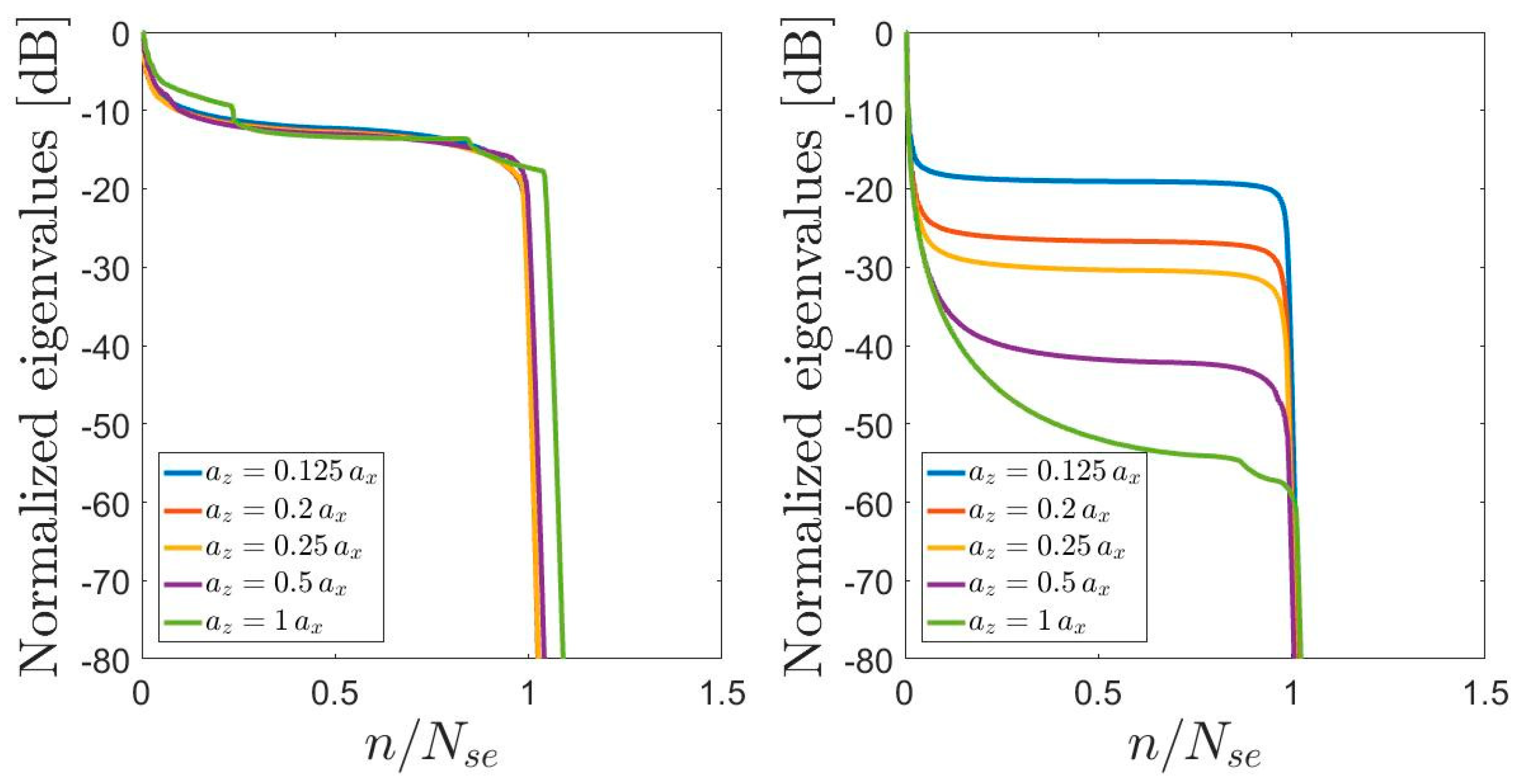
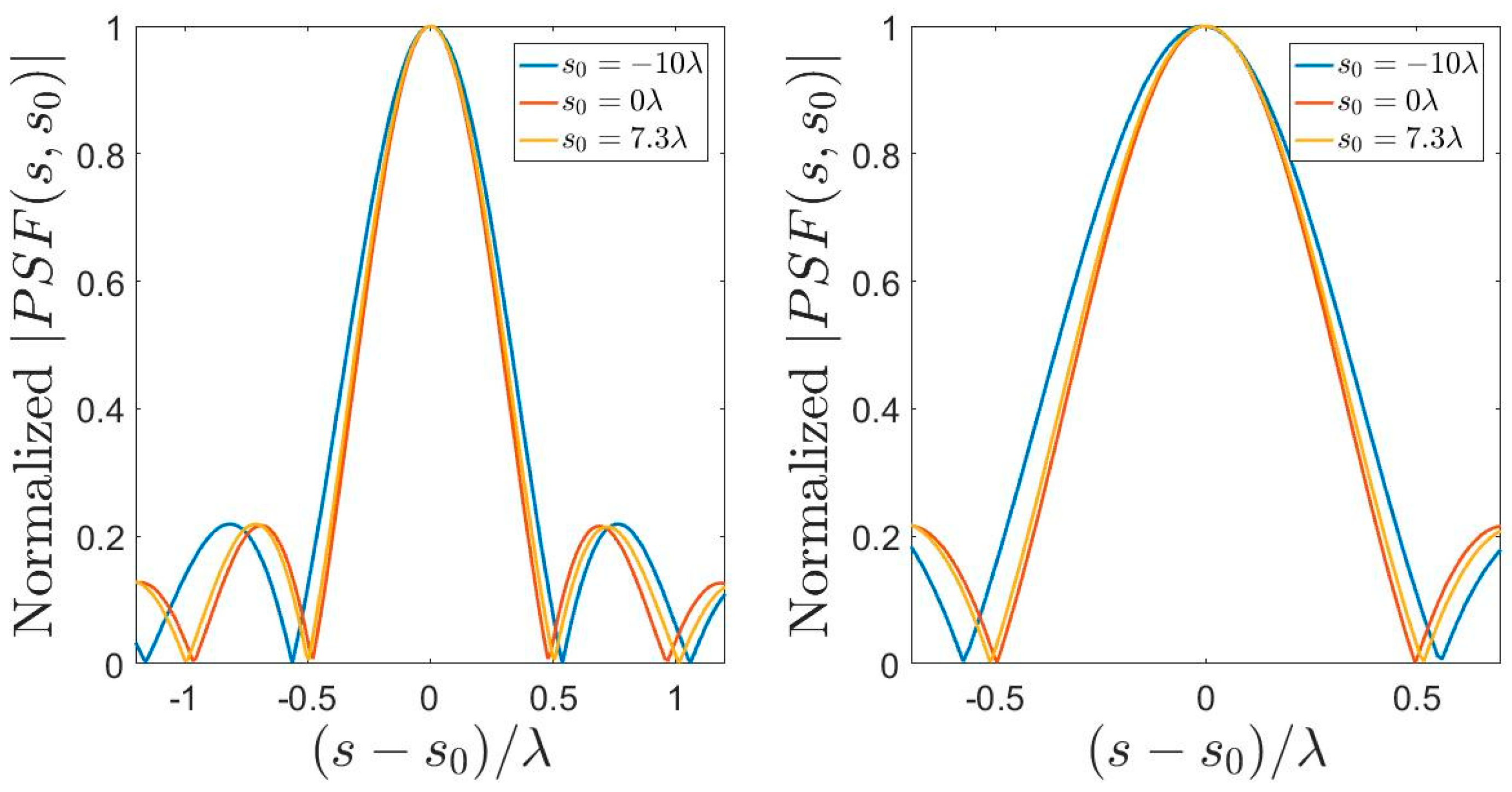
3.3. Semi-Elliptic Source

For a semi-elliptic source (Figure 8), the radiated field is given by

$$\mathrm{E}\left(\mathsf{\theta }\right)=\underset{-\mathsf{\pi }/2}{\overset{\mathsf{\pi }/2}{{\displaystyle \int }}}\mathrm{J}\left(\mathsf{\varphi }\right){\mathrm{e}}^{\mathrm{j}\mathsf{\beta }\left({\mathrm{a}}_{\mathrm{x}}\sin \mathsf{\varphi }\sin \mathsf{\theta }+{\mathrm{a}}_{\mathrm{z}}\cos \mathsf{\varphi }\cos \mathsf{\theta }\right)}\sqrt{{\mathrm{a}}_{\mathrm{x}}^2{\cos }^2\mathsf{\varphi }+{\mathrm{a}}_{\mathrm{z}}^2{\sin }^2\mathsf{\varphi }} \mathrm{d}\mathsf{\varphi }={ℒ}_{\mathsf{\theta }}\left(\mathrm{J}\right),$$

(15)

and

$$\mathrm{E}\left(\mathrm{u}\right)={\mathrm{a}}_{\mathrm{x}}\underset{-1}{\overset{1}{{\displaystyle \int }}}\mathrm{J}\left(\mathrm{x}\right){\mathrm{e}}^{\mathrm{j}\mathsf{\beta }\left[{\mathsf{\xi }\mathrm{a}}_{\mathrm{x}}\mathrm{u}+{\mathrm{a}}_{\mathrm{z}}\sqrt{1-{\mathsf{\xi }}^2} \sqrt{1-{\mathrm{u}}^2}\right]} \sqrt{1+\frac{{\mathrm{a}}_{\mathrm{z}}^2}{{\mathrm{a}}_{\mathrm{x}}^2}\frac{{\mathsf{\xi }}^2}{1-{\mathsf{\xi }}^2}}\mathrm{d}\mathsf{\xi }={ℒ}_{\mathrm{u}}\left(\mathrm{J}\right).$$

(16)

An extensive numerical analysis provides us an approximated estimation of the NDF as

$${\mathrm{N}}_{\mathrm{se}}\approx \left[\frac{4{\mathrm{a}}_{\mathrm{x}}}{\mathsf{\lambda }}+\frac{{\mathrm{a}}_{\mathrm{z}}}{\mathsf{\lambda }}\right],$$

(17)

as shown in Figure 9 and Figure 10, where the normalized eigenvalues are plotted with respect to indices normalized to ${\mathrm{N}}_{\mathrm{se}}$ for different choices of ${\mathrm{a}}_{\mathrm{x}}$ and aspect ratio ${\mathrm{a}}_{\mathrm{x}}/{\mathrm{a}}_{\mathrm{z}}$. We can appreciate from the figures that the introduced value ${\mathrm{N}}_{\mathrm{se}}$ approximately corresponds to the number of significant eigenvalues. (In Appendix A, we provide a rough analysis about the observed behavior (17)).

Thus, for a semi-elliptic source observed on a semi-circumference, the number of relevant eigenvalues may be connected to the source extension along both the x and z axes. In particular, the semi-axis ${\mathrm{a}}_{\mathrm{x}}$ contributes to the NDF as a linear source. In turn, the semi-axis ${\mathrm{a}}_{\mathrm{z}}$ acts as a linear source four times smaller for symmetry reasons: we are just considering a half ellipse, and this leads to a first reduction of the NDF to a half with respect to the case of a $2{\mathrm{a}}_{\mathrm{z}}$ long linear source. Moreover, the observation domain is symmetric with respect to the z-directed line source, further halving the contribution to the NDF.

Equation (17) reveals that the NDF increases by decreasing the aspect ratio of the source, implying that as soon as the source evolves from a line to a semi-circumference, the NDF increases.

From Figure 9 and Figure 10, it can be appreciated, first, how the step of the eigenvalue curve is close to the one predicted for the linear source as long as the aspect ratio of the semi-elliptic source is large, as expected. Moreover, as long as ${\mathrm{a}}_{\mathrm{z}}\le {\mathrm{a}}_{\mathrm{x}}$, Equation (17) still represents a useful upper bound for the number of significant eigenvalues, providing an estimate more accurate than (13) (if we consider the smallest circumference enclosing the source). For example, when ${\mathrm{a}}_{\mathrm{x}}=10\mathsf{\lambda }$ and ${\mathrm{a}}_{\mathrm{z}}=5\mathsf{\lambda }$, the step occurs for $\mathrm{n}=45,$ while the value returned by (13) is 62.

Finally, for ${\mathrm{a}}_{\mathrm{x}}={\mathrm{a}}_{\mathrm{z}}=10\mathsf{\lambda }$, i.e., for a semicircular source, the number foretold by Equation (17) is 50 against an upper bound of 62 predicted by Equation (13). Similarly, for ${\mathrm{a}}_{\mathrm{x}}={\mathrm{a}}_{\mathrm{z}}=100\mathsf{\lambda }$, Equation (17) returns 500, while Equation (13) returns 628. Therefore, in any case, by accounting for the source geometry, (17) provides a more accurate estimate of the NDF.

Another important point to be stressed is that the number of significant eigenvalues is approximately the same for both the operators ${ℒ}_{\mathrm{u}}$ and ${ℒ}_{\mathsf{\theta }}$, as it occurs for a linear source. This means that the NDF does not depend on the observation variable. However, the set of eigenfunctions may differ. A way to investigate this point requires the evaluation of the PSF.

Referring to the variables used in the definition of operators (15) and (16), for both of the variables choices, the PSF is not available in an analytic form, but results of numeric simulations can be discussed. Since the operators ${ℒ}_{\mathsf{\theta }}^{†}{ℒ}_{\mathsf{\theta }}$ and ${ℒ}_{\mathrm{u}}^{†}{ℒ}_{\mathrm{u}}$ have no convolutional kernels, we expect spatially variant PSFs.

In Figure 11, the PSFs for both the sets of variables are shown. We can see that the width of the main lobes is spatially variant, and accordingly, the resolution has the same behavior as above.

In order to make a comparison between the PSFs, we can again introduce the arc length defined as

$$\mathrm{s}\left(\mathsf{\varphi }\right)=\mathrm{s}\left(-\mathsf{\alpha }\right)+{{\displaystyle \int }}_{-\mathsf{\alpha }}^{\mathsf{\varphi }}||{\mathsf{\gamma }}^{\prime }\left(\mathrm{t}\right)||\mathrm{dt},$$

(18)

where $\mathrm{s}\left(-\mathsf{\alpha }\right)$ is chosen to be minus the semi-length of the source. Again, we can observe that once we plot the PSFs with respect to the arc length, the PSF in the source domain is more invariant.

Moreover, while in Figure 11 the choice of the source variable seems to imply a difference in the resolution (especially close to the end points), by adopting the representation in terms of the arc length variable, the previous difference disappears. The overlapped PSFs for the two operators are shown in Figure 12. We can note that, while at a first sight the resolution may appear spatially invariant, it changes slightly with the abscissa. This time, in contrast to the semi-circumference case, the link between the $\mathsf{\varphi }$ and $\mathrm{s}$ variables is not linear, implying a different behavior for the PSFs. For the displayed PSFs, we find that for the operator ${ℒ}_{\mathsf{\theta }},$ the percentage variation of the main lobe width normalized to the maximum value is about 48% in the $\mathsf{\varphi }$ variable and 13% in the $\mathrm{s}$ one. For the operator ${ℒ}_{\mathsf{\theta }}$, it is about 27% in the $\mathsf{\xi }$ variable and 13% in the $\mathrm{s}$ one. Once again, the arc length variable assures a more invariant resolution along the considered domain.

4. Discussion of the Results

The examined scenario of a semi-elliptic source observed in the far zone over a semi-circumference allows a discussion about how a changing aspect ratio of the current source and a different variables choice affect NDF and PSF behavior. Regarding the NDF, we can state that:

• For a fixed $x$ extension of the source, increasing the $z$ dimension leads to an increase of the NDF dictated by (17).
• The NDF does not depend on the choice of the variables considered in this study.
• Equation (17) returns a more accurate estimation for the NDF of a semi-circumference source with respect to the upper bound (13) provided by [27].

The main results about the PSF are the following:

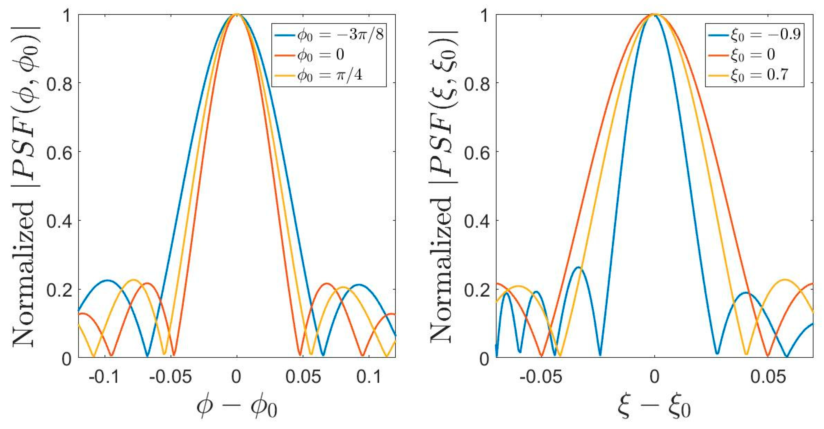
• Except for the limit case of a linear source that presents an invariant PSF for both the considered variable choices, increasing the $z$ dimension of the source leads to a variant PSF along the source domain, independent of the variables choice.
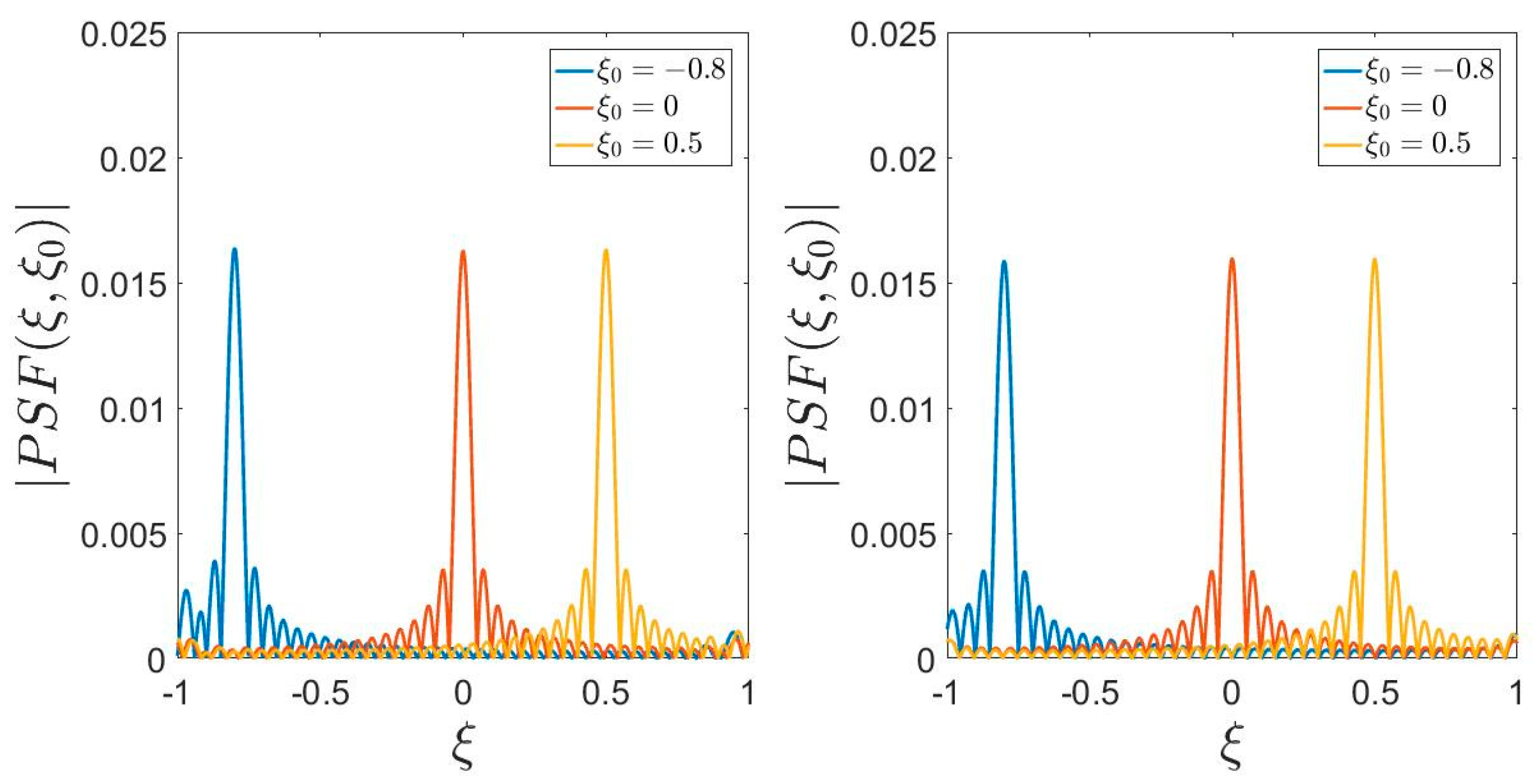
• The PSF is always variant along the observation domain, independent of the considered variables choice.
• Among all the possible variables choices discussed in this paper, the one ensuring a more invariant PSF is the arc length.

These results may be of large interest not only in source reconstruction for diagnostic purposes but also in reducing field measurements in antenna testing since the actual independence of the NDF from the choices of both source and observation variables reveals that a minimum number of measurement points can be introduced.

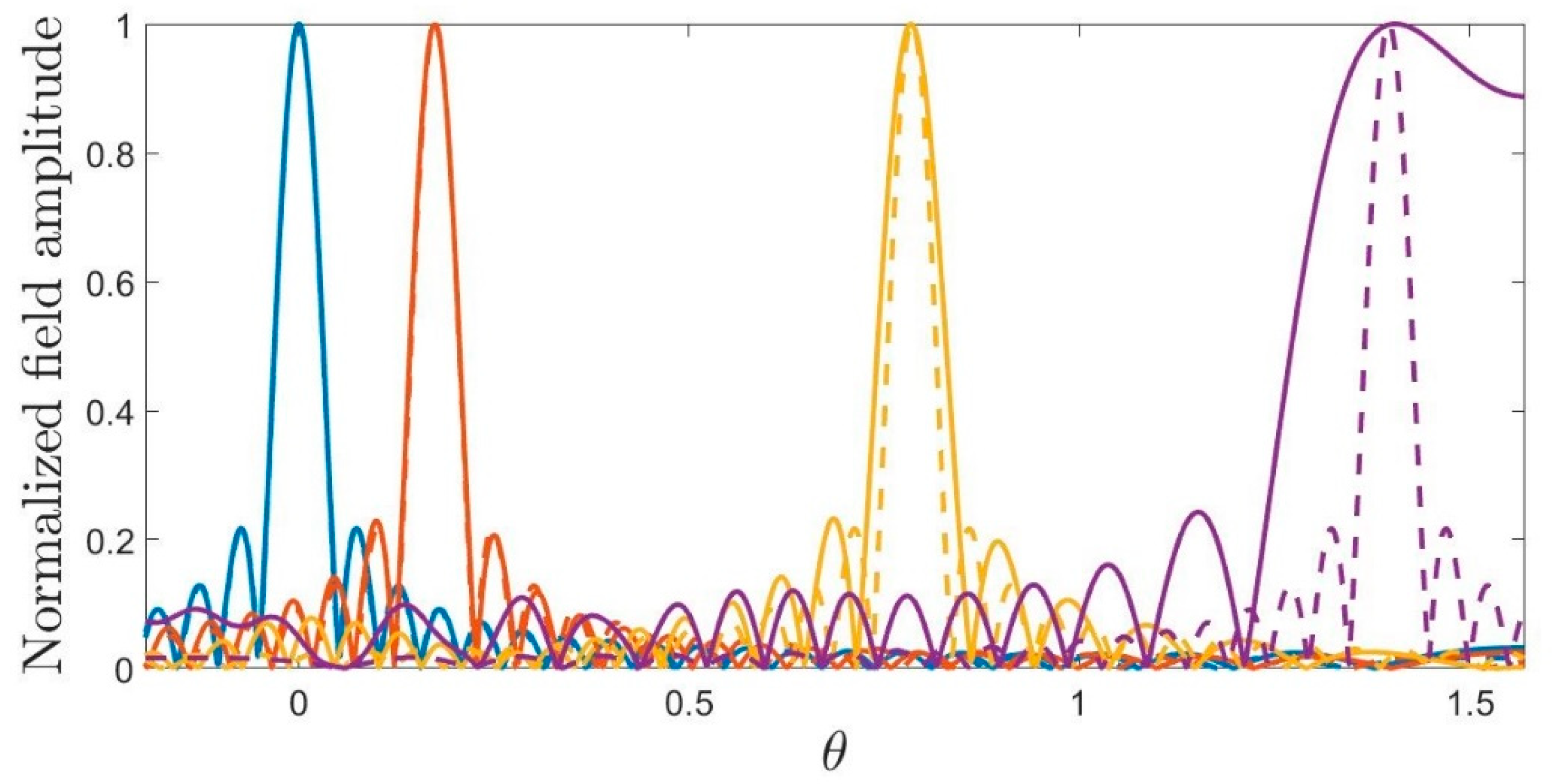
5. Examples of Antenna Applications

In the following sections, we point out the role of the source geometry in some antenna applications, with a focus on the NDF and the PSF of the relevant operators. In fact, the knowledge of their eigendecomposition may provide useful pieces of information about both the capacity of the source to radiate a prescribed set of radiation patterns and the kinds of sources that can be reconstructed with an assigned accuracy in the presence of uncertainties in data.

To show this, we deal with the reconstruction of the excitation of antenna array elements for diagnostic purposes (Section 5.1) and the capacity of the analyzed geometries to radiate an identical focusing pattern pointing at different directions to achieve a uniform coverage within a prescribed angular sector (Section 5.2).

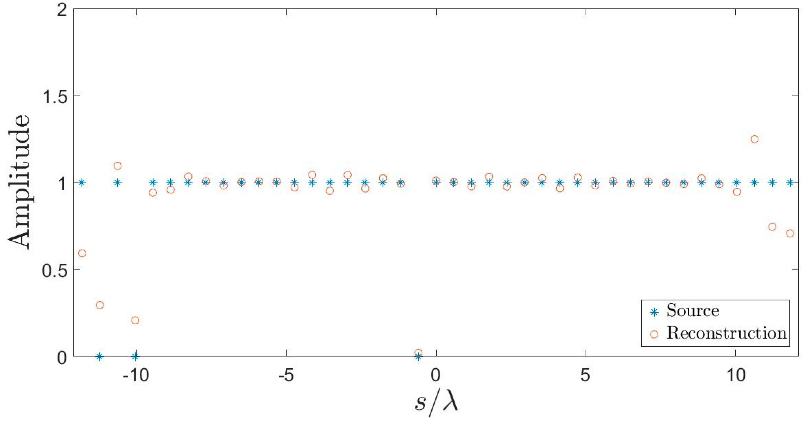
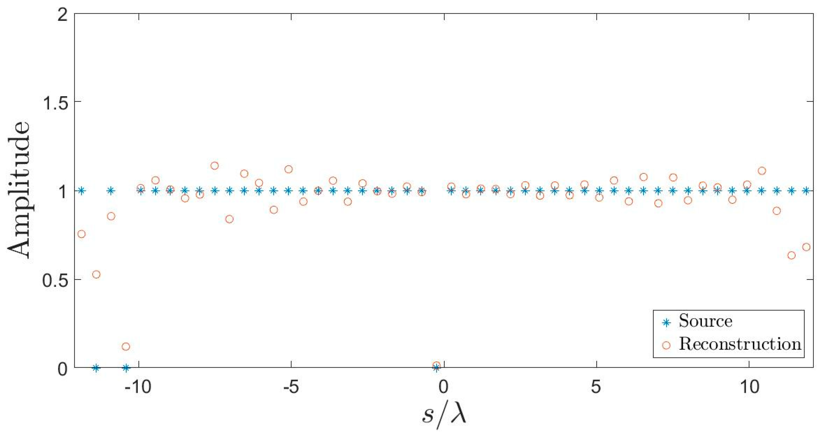
5.1. Array Diagnostics

The utility of knowing the NDF for a given current source can be well understood in application contexts such as array diagnostics. As discussed above, the NDF is related to the size of the functional space of the sources that can be stably reconstructed and therefore, can be connected to the practical need of reconstructing the excitations of an antennas array and possibly of identifying faulty elements.

In addition, the knowledge of the PSF’s behavior could be useful to predict the accuracy of the diagnostic results according to the considered source shape. In fact, if the PSF was invariant along the source domain, we would be able to reconstruct, with a fixed accuracy, a number of equally spaced sources equal or less than the NDF, independently of their position. On the contrary, as discussed in Section 3, when the PSF exhibits a space-variant behavior, reconstructions with different resolutions along the source domain can be expected. To fix the ideas, if we consider a semi-elliptic source geometry and the results in Figure 12 for operator ${ℒ}_{\mathsf{\theta }}$, we can see that the PSF main lobe becomes wider towards the end of the source domain. Hence, reconstructions of the excitations of two closer array elements located at the extremal side of the curve are expected to be worst, while it may be satisfactory when the elements are located towards the middle of the array source.

In order to numerically verify these points, let us suppose that the array elements are filamentary sources fed with unit amplitude currents. These elements are located along a semi-ellipse with ${\mathrm{a}}_{\mathrm{x}}=10\mathsf{\lambda }$ and ${\mathrm{a}}_{\mathrm{z}}=5\mathsf{\lambda }$, and uniformly spaced in the $\mathrm{s}$ arc length variable at $\mathsf{\Delta }\mathrm{s}$ step. The radiated field is collected with a sufficiently dense grid (let’s say twice the NDF) at uniform $\mathsf{\theta }$ step over a semi-circumference in the far zone. The field radiated by such a discrete source is provided by the following relationship:

$$\mathrm{E}\left(\mathsf{\theta }\right)={\displaystyle \sum }_{\mathrm{n}=1}^{\mathrm{N}}{\mathrm{a}}_{\mathrm{n}}{ \mathrm{e}}^{\mathrm{j}\mathsf{\beta }\left[\mathrm{x}\left(\mathrm{n}\mathsf{\Delta }\mathrm{s}\right)\sin \mathsf{\theta }+\mathrm{z}\left(\mathrm{n}\mathsf{\Delta }\mathrm{s}\right)\cos \mathsf{\theta }\right]},$$

(19)

where the ${\mathrm{a}}_{\mathrm{n}}$ coefficient is the excitation of the n-th source and $\mathrm{N}$ is the number of filamentary sources used in the examples.

From the left panel of Figure 12, if we assume the 0.5 level of the PSFs as the main lobe width, we expect that when the elements’ spacing is larger than it, the feeding currents of the elements may not be perfectly reconstructed. Moreover, this situation may occur when the number of array elements along the semi-ellipse is greater than the NDF.

Figure 13 refers to a 50-element array, i.e., larger than the NDF, and the reconstruction worsens for the lateral elements of the array so that diagnostics of the faulty elements can be wrong. In fact, the width of the PSFs at a 0.5 level for ${\mathrm{s}}_0=-10\mathsf{\lambda }$ and ${\mathrm{s}}_0=0$ is equal to $0.65\mathsf{\lambda }$ and $0.58\mathsf{\lambda },$ respectively, which is higher than $0.48\mathsf{\lambda }$, the spacing between two adjacent elements.

On the contrary, if the total number of array elements is lower than the estimated NDF of the source, the reconstruction algorithm works better (see Figure 14), especially at the center of the array where the PSF main lobe assumed width is lower than the distance between two adjacent elements, that is, $0.59\mathsf{\lambda }$.

For both reconstructions in Figure 13 and Figure 14, the truncated SVD algorithm is adopted for the inversion of operator (19) and we retain the singular functions corresponding to normalized singular values higher than −10 dB.

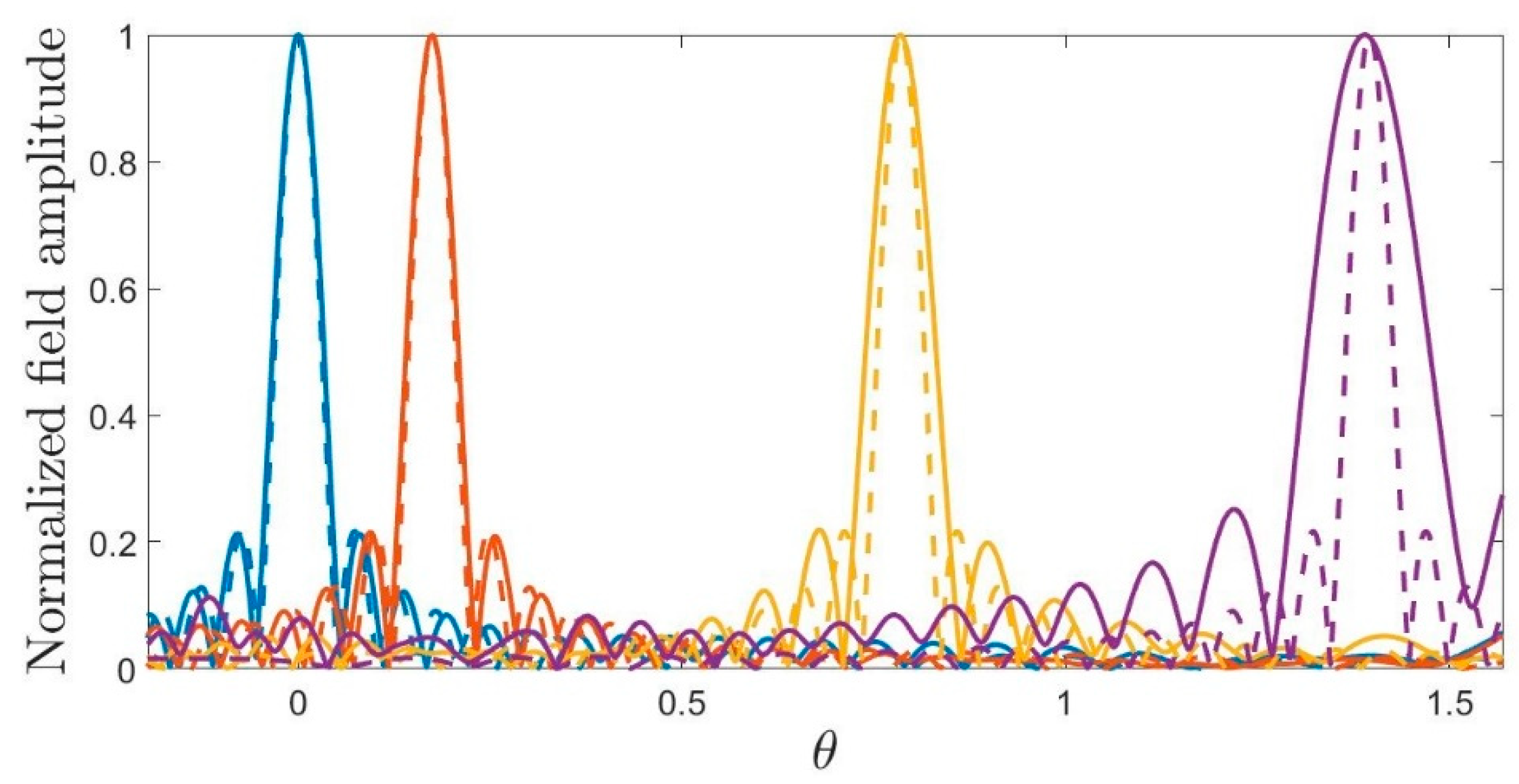
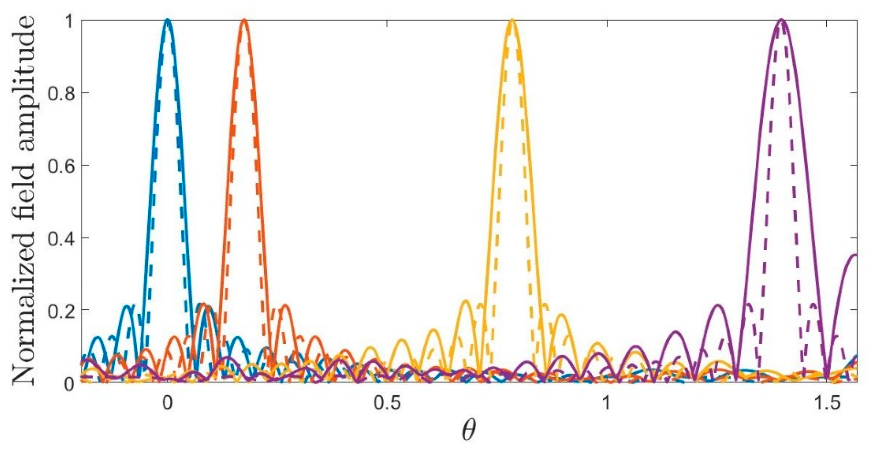
5.2. Pattern Synthesis

Some surveillance radar applications require the antenna system to radiate identical beams pointing at different directions within a prescribed angular range. Hereafter, we address this example by comparing three different 2D source geometries, i.e., a line, a semi-circumference, and a semi-ellipse, through the examination of the corresponding eigenfunctions spanning the observation domain. In particular, in order to get general information about them, we resort to a “spectral content” function defined as

$$\mathrm{SC}\left(\mathsf{\theta }\right)={\displaystyle \sum }_{\mathrm{i}=1}^{{\mathrm{N}}_{\mathrm{T}}}{|{\mathrm{v}}_{\mathrm{i}}\left(\mathsf{\theta }\right)|}^2,$$

(20)

where ${\mathrm{N}}_{\mathrm{T}}$ represents the number of retained eigenfunctions.

In order to make a fair comparison between the subspaces, the following discussion is performed by holding the same ${\mathrm{N}}_{\mathrm{T}}$, i.e., the subspace dimension (chosen as the eigenvalues index where the step occurs), for all the geometries, implying that, now, both the source extensions along the $\mathrm{x}$ and $\mathrm{z}$ axes may change from a linear source to a semi-circumference. Figure 15 reports the spectral content, $\mathrm{SC}\left(\mathsf{\theta }\right)$, functions for the operator ${ℒ}_{\mathsf{\theta }}$ in the observation domain $\mathsf{\theta }\in \left[-\mathsf{\pi }/2,\mathsf{\pi }/2\right]$.

It can be appreciated that the ratio between the maximum and minimum value of $\mathrm{SC}\left(\mathsf{\theta }\right)$ is smaller for a semi-circumference and higher for a linear source. Therefore, we can expect that the semi-circumference source would be able to radiate a given field along a wider observation domain than the others, on average.

Just to fix the ideas, we consider as the desired field the one radiated for small angles by a linear source with ${\mathrm{N}}_{\mathrm{T}}$ degrees of freedom, that is,

$$\mathrm{E}(\mathsf{\theta })=\sin \mathrm{c}({\mathsf{\beta }\mathrm{a}}_{\mathrm{x}}^{\prime }(\mathsf{\theta }-{\mathsf{\theta }}_0)),$$

(21)

where ${\mathsf{\theta }}_0$ is the maximum angle, and ${\mathrm{N}}_{\mathrm{T}}=[2{\mathsf{\beta }\mathrm{a}}_{\mathrm{x}}^{\prime }/\mathsf{\pi }]$. The best approximation of (21) in quadratic norm is provided by the projection onto the subspace of the significant eigenfunctions characterizing each geometry. Accordingly, the projected field $\tilde{\mathrm{E}}(\mathsf{\theta })$ is computed as

$$\tilde{\mathrm{E}}(\mathsf{\theta })={\displaystyle \sum }_{\mathrm{n}=1}^{{\mathrm{N}}_{\mathrm{T}}}{\mathrm{e}}_{\mathrm{n}}{\mathrm{v}}_{\mathrm{n}}(\mathsf{\theta }),$$

(22)

where the coefficients ${\mathrm{e}}_{\mathrm{n}}$ are given by the scalar product

$${\mathrm{e}}_{\mathrm{n}}={{\displaystyle \int }}_{-\mathsf{\pi }/2}^{\mathsf{\pi }/2}\mathrm{E}(\mathsf{\theta }) {\mathrm{v}}_{\mathrm{n}}^{*}(\mathsf{\theta })\hspace{0.17em}\mathrm{d}\mathsf{\theta }.$$

(23)

The projected fields $\tilde{\mathrm{E}}\left(\mathsf{\theta }\right)$ are reported in Figure 16, Figure 17 and Figure 18.

In order to compare the capability to radiate the pattern provided by (21) along different maximum directions, we adopt as figures of merit both the half power beam width (HPBW), that is, the angular interval where the magnitude of the radiation pattern decreases by 50% (or −3 dB) from the peak, and the achieved directivity

$$\mathrm{D}\left({\mathsf{\theta }}_0\right)=\frac{{|\tilde{\mathrm{E}}\left({\mathsf{\theta }}_0\right)|}^2}{\frac{1}{\mathsf{\pi }}{{\displaystyle \int }}_{-\mathsf{\pi }/2}^{\mathsf{\pi }/2}{|\tilde{\mathrm{E}}\left(\mathsf{\theta }\right)|}^2\hspace{0.17em}\mathrm{d}\mathsf{\theta }}.$$

(24)

Table 1. Half power beam width (HPBW) of the desired field and projected field for a linear, semi-elliptical, and semi-circumference source, varying the main beam angle ${\mathsf{\theta }}_0$.

HPBW	Linear source (rad)	Semi-ellipse (rad)	Semi-circumference (rad)	Assigned pattern (rad)
${\mathsf{\theta }}_0=0 \mathrm{rad}$	0.043	0.047	0.056	0.043
${\mathsf{\theta }}_0=0.17 \mathrm{rad}$	0.045	0.049	0.054	0.043
${\mathsf{\theta }}_0=0.78 \mathrm{rad}$	0.063	0.065	0.065	0.043
${\mathsf{\theta }}_0=1.4 \mathrm{rad}$	0.267	0.117	0.092	0.043

reports the HPBW for the considered geometries. From the numerical results, it is clear that the main lobe widens by moving from the center of the observation domain to the extremal points, as expected from Figure 15, where the $\mathrm{SC}\left(\mathsf{\theta }\right)$ functions, generally, decrease toward $\mathsf{\theta }=\pm \mathsf{\pi }/2$. Moreover, the linear source can match the assigned field better for lower ${\mathsf{\theta }}_0$ than for higher ones. In contrast, the main lobe widths enlarge to a lesser extent for the semi-ellipse and the semi-circumference geometries.

Table 2. Directivity in dB of the projected field for a linear, semi-elliptical, and semi-circumference sources, varying the main beam angle ${\mathsf{\theta }}_0$.

D	Linear source (dB)	Semi-ellipse (dB)	Semi-circumference (dB)	Assigned pattern (dB)
${\mathsf{\theta }}_0=0 \mathrm{rad}$	35.60	34.93	33.65	35.76
${\mathsf{\theta }}_0=0.17 \mathrm{rad}$	35.57	34.78	33.67	35.77
${\mathsf{\theta }}_0=0.78 \mathrm{rad}$	32.74	32.27	32.26	35.77
${\mathsf{\theta }}_0=1.4 \mathrm{rad}$	21.75	27.42	29.45	35.88

presents the dB values of the directivity for the three considered shapes. Consistent with the behavior of the $\mathrm{SC}\left(\mathsf{\theta }\right)$ function, we obtain a pretty high value of the maximum directivity within the interval ${\mathsf{\theta }}_0\in \left[-\mathsf{\pi }/4,\mathsf{\pi }/4\right]$ for all the geometries, while the directivity worsens towards the end point directions, especially for the linear source.

6. Conclusions

The role of the geometry in the inverse source reconstruction problem for far zone data has been examined by referring to a semi-elliptic source when the observation domain is a semi-circumference. A good estimation for the NDF is provided, while a PSF analysis shows that limited sources and observations make the PSFs variant along the domains, even if we use different representation variables.

The capacity to reconstruct point-like sources has been also considered in connection with the array antenna diagnostics problem. In fact, the PSF can define the minimum resolution in discriminating two close sources, as numerical examples about conformal array diagnostics reveal.

Finally, the role of the source geometry in an antenna synthesis problem is emphasized by comparing the radiation patterns radiated by three different sources when identical focusing beams are required along a wide angular domain.

References

1. Josefsson, L.; Persson, P. Conformal Array Antenna Theory and Design; John Wiley & Sons: Hoboken, NJ, USA, 2006. [Google Scholar]
2. Semkin, V.; Ferrero, F.; Bisognin, A.; Ala-Laurinaho, J.; Luxey, C.; Devillers, F.; Räisänen, A.V. Beam Switching Conformal Antenna Array for mm-Wave Communications. IEEE Antennas Wirel. Propag. Lett. 2016, 15, 28–31. [Google Scholar] [CrossRef]
3. Wang, Z.; Hall, P.S.; Kelly, J.R.; Gardner, P. Wideband Frequency-Domain and Space-Domain Pattern Reconfigurable Circular Antenna Array. IEEE Trans. Antennas Propag. 2017, 65, 5179–5189. [Google Scholar] [CrossRef]
4. Rodriguez-Gonzalez, J.A.; Ares-Pena, F.; Fernandez-Delgado, M.; Iglesias, R.; Barro, S. Rapid method for finding faulty elements in antenna arrays using far field pattern samples. IEEE Trans. Antennas Propag. 2009, 57, 1679–1683. [Google Scholar] [CrossRef]
5. Carlin, M.; Oliveri, G.; Massa, A. On the robustness to element failures of linear ADS-thinned arrays. IEEE Trans. Antennas Propag. 2011, 59, 4849–4853. [Google Scholar] [CrossRef]
6. Buonanno, A.; D’urso, M. On the diagnosis of arbitrary geometry fully active arrays. In Proceedings of the Fourth European Conference on Antennas and Propagation, Barcelona, Spain, 12–16 April 2010. [Google Scholar]
7. Cappellin, C.; Meincke, P.; Pivnenko, S.; Jorgensen, E. Array antenna diagnostics with the 3D reconstruction algorithm. In Proceedings of the 34th Annual Symposium of the Antenna Measurement Techniques Association, Bellevue, WA, USA, 21–26 October 2012. [Google Scholar]
8. Cheng, G.G.; Zhu, Y.; Grzesk, J. Exact solutions in antenna holography using planar spherical or cylindrical near-field data. In Proceedings of the 34th Annual Symposium of the Antenna Measurement Techniques Association, Bellevue, WA, USA, 21–26 October 2012. [Google Scholar]
9. Schnattinger, G.; Eibert, T.F. 3D image generation from arbitrary antenna measurement data by solving the full vectorial inverse source problem. In Proceedings of the 34th Annual Symposium of the Antenna Measurement Techniques Association, Bellevue, WA, USA, 21–26 October 2012. [Google Scholar]
10. Bucci, O.M.; Migliore, M.D.; Panariello, G.; Sgambato, P. Accurate diagnosis of conformal arrays from near-field data using the matrix method. IEEE Trans. Antennas Propag. 2005, 53, 1114–1120. [Google Scholar] [CrossRef]
11. Patnaik, A.; Choudhury, B.; Pradhan, P.; Mishra, R.K.; Christoulou, C. An ANN application for fault finding in antenna arrays. IEEE Trans. Antennas Propag. 2007, 55, 775–777. [Google Scholar] [CrossRef]
12. Brégains, J.C.; Ares, F. Matrix pseudo-inversion technique for the diagnostics of planar arrays. In Proceedings of the First European Conference on Antennas and Propagation, Nice, France, 6–10 November 2006. [Google Scholar]
13. Oliveri, G.; Rocca, P.; Massa, A. Reliable diagnosis of large linear arrays—A Bayesian compressive sensing approach. IEEE Trans. Antennas Propag. 2012, 60, 4627–4636. [Google Scholar] [CrossRef]
14. LaHaie, I.J.; Cossmann, S.M.; Blischke, M.A. A Model-Based Technique with ℓ 1 Minimization for Defect Detection and RCS Interpolation from Limited Data. Appl. Comput. Electromagn. Soc. J. 2013, 28, 1171–1178. [Google Scholar]
15. Di Francia, G.T. Degrees of freedom of an image. J. Opt. Soc. Am. 1969, 59, 799–804. [Google Scholar] [CrossRef]
16. Miller, D.A. Communicating with waves between volumes: Evaluating orthogonal spatial channels and limits on coupling strengths. Appl. Opt. 2000, 39, 1681–1699. [Google Scholar] [CrossRef]
17. Piestun, R.; Miller, D.A. Electromagnetic degrees of freedom of an optical system. J. Opt. Soc. Am. A 2000, 17, 892–902. [Google Scholar] [CrossRef]
18. Somaraju, R.; Trumpf, J. Degrees of freedom of a communication channel: Using DOF singular values. IEEE Trans. Inf. Theory 2010, 56, 1560–1573. [Google Scholar] [CrossRef]
19. Frazin, R.A.; Fischer, D.G.; Carney, P.S. Information content of the near field: Two-dimensional samples. J. Opt. Soc. Am. A 2004, 21, 1050–1057. [Google Scholar] [CrossRef]
20. Fischer, D.G.; Frazin, R.A.; Asipauskas, M.; Carney, P.S. Information content of the near field: Three-dimensional samples. J. Opt. Soc. Am. A 2011, 28, 296–306. [Google Scholar] [CrossRef]
21. Solimene, R.; Maisto, M.A.; Pierri, R. Information Content in Inverse Source with Symmetry and Support Priors. Prog. Electromagn. Res. 2018, 80, 39–54. [Google Scholar] [CrossRef]
22. Bertero, M.; Boccacci, P. Introduction to Inverse Problems in Imaging; IOP Publishing: Bristol, UK, 1998. [Google Scholar]
23. Newsam, G.; Barakat, R. Essential dimension as a well-defined number of degrees of freedom of finite-convolution operators appearing in optics. J. Opt. Soc. Am. A 1985, 2, 2040–2045. [Google Scholar] [CrossRef]
24. Den Dekker, A.J.; van den Bos, A. Resolution: A survey. J. Opt. Soc. Am. A 1997, 14, 547–557. [Google Scholar] [CrossRef]
25. Leone, G. Source Geometry Optimization for Hemispherical Radiation Pattern Coverage. IEEE Trans. Antennas Propag. 2016, 64, 2033–2038. [Google Scholar] [CrossRef]
26. Leone, G.; Maisto, M.A.; Pierri, R. “Application of Inverse Source Reconstruction to Conformal Antennas Synthesis. IEEE Trans. Antennas Propag. 2018, 66, 1436–1445. [Google Scholar] [CrossRef]
27. Leone, G.; Maisto, M.A.; Pierri, R. Inverse Source of Circumference Geometries: SVD Investigation based on Fourier Analysis. Prog. Electromagn. Res. 2018, 76, 217–230. [Google Scholar] [CrossRef]
28. Slepian, D.; Pollack, H.O. Prolate spheroidal wave functions, Fourier analysis, and uncertainty—I. Bell Syst. Techn. J. 1961, 40, 43–63. [Google Scholar] [CrossRef]
29. Landau, H.J.; Pollack, H.O. The eigenvalue distribution of time and frequency limiting. J. Math. Phys. 1980, 77, 469–481. [Google Scholar] [CrossRef]
Figure 1. Linear source geometry.
Electronics 08 00531 g001
Figure 2. The point spread functions (PSFs) of the operators ^ θ (left panel) and u (right panel) of a linear source with a x = 10   λ , for ξ 0 = 0.8 ,   0 ,   0.5 .
Electronics 08 00531 g002
Figure 3. The PSF in the observation domain of the operator ^ θ of a linear source with a x = 10 λ , for θ 0 = 3 π / 8 ,   0 ,   π / 4 .
Electronics 08 00531 g003
Figure 4. Semi-circumference source geometry.
Electronics 08 00531 g004
Figure 5. Normalized eigenvalues of the operators θ (left panel) and u (right panel) for a semi-circumference source varying the radius.
Electronics 08 00531 g005
Figure 6. Normalized and overlapped PSFs of θ (left panel) and u (right panel) operators   of a semi-circumference source with a x = 10 λ for ϕ 0 = 3 π / 8 ,   0 , π / 4 and for the corresponding values ξ 0 = 0.9 ,   0 ,   0.7 .
Electronics 08 00531 g006
Figure 7. Normalized and overlapped PSFs of θ (left panel) and u (right panel) operators   of a semi-circumference source with a x = 10 λ plotted in function of the arc length variable (the s 0 values are computed in correspondence to the ϕ 0 and ξ 0 used in Figure 6).
Electronics 08 00531 g007
Figure 8. Semi-elliptic source geometry.
Electronics 08 00531 g008
Figure 9. Normalized eigenvalue behaviors (reported in descending order) of θ (left panel) and u (right panel) operators for a semi-elliptic source when a x = 10 λ . Each line refers to a different aspect ratio a x / a z .
Electronics 08 00531 g009
Figure 10. Normalized eigenvalue behaviors (reported in descending order) of θ (left panel) and u (right panel) operators for a semi-elliptic source when a x = 100 λ . Each line refers to a different aspect ratio a x / a z .
Electronics 08 00531 g010
Figure 11. Normalized and overlapped PSFs of θ (left panel) and u (right panel) operators of a semi-elliptic source, with a x = 10 λ and a z = 5 λ , for ϕ 0 = 3 π / 8 ,   0 , π / 4 and for the corresponding values ξ 0 = 0.9 ,   0 ,   0.7 .
Electronics 08 00531 g011
Figure 12. The overlapped and normalized PSFs of θ (left panel) and u (right panel) operators of a semi-elliptic source with a x = 10 λ and a z = 5 λ , plotted in function of the arc length variable (the s 0 values are computed in correspondence to the ϕ 0 and ξ 0 used in Figure 11).
Electronics 08 00531 g012
Figure 13. Reconstruction of a 50-element array with two faulty elements. The number of array elements is larger than the one estimated by (17) as the source NDF (45).
Electronics 08 00531 g013
Figure 14. Reconstruction of a 41-element array with two faulty elements. The number of array elements is smaller than the one estimated by (17) as the source NDF (45).
Electronics 08 00531 g014
Figure 15. Spectral content functions SC ( θ ) for a linear source ( a x = 9.75   λ ), a semi-ellipse ( a x = 8.75   λ and a z = 5   λ ), and a semi-circumference ( a x = a z = 7.4   λ ) with the same number of significant eigenvalues ( N T = 40 ).
Electronics 08 00531 g015
Figure 16. Normalized field amplitude of the desired field E ( θ ) (dashed curves) and the projected field E ˜ ( θ ) (solid curves) for the linear source, varying the main beam angle θ 0 = 0 ,   0.17 ,   0.78 ,   1.4 . The panels only zoom into a portion of the observation domain.
Electronics 08 00531 g016
Figure 17. Normalized field amplitude of the desired field E ( θ ) (dashed curves) and the projected field E ˜ ( θ ) (solid curves) for the semi-elliptic source, varying the main beam angle θ 0 = 0 ,   0.17 ,   0.78 ,   1.4 . The panels only zoom into a portion of the observation domain.
Electronics 08 00531 g017
Figure 18. Normalized field amplitude of the desired field E ( θ ) (dashed curves) and the projected field E ˜ ( θ ) (solid curves) for the semi-circumference source, varying the main beam angle θ 0 = 0 ,   0.17 ,   0.78 ,   1.4 . The panels only zoom into a portion of the observation domain.
Electronics 08 00531 g018