Abstract
In classification and localization of mixed far-field and near-field sources, the unknown mutual coupling degrades the performance of most high-resolution algorithms. In practice, the assumption of an ideal receiving sensor array is rarely satisfied. This paper proposes an effective algorithm of mixed sources identification using uniform circular array under unknown mutual coupling. Firstly, according to rank reduction and joint space–time processing, the directions of arrival of far-field sources is estimated directly without mutual coupling elimination. Addition, the joint space–time processing can improve the estimation results in the case of low signal noise ratio of incoming signal sources and small number of snapshots. Then, these estimates are adopted to reconstruct the mutual coupling matrix. Finally, both direction and range parameters of near-field sources are obtained through spatial search after mutual coupling effects and far-field components elimination. The proposed algorithm is described in detail, and its behavior is illustrated by numerical examples.
1. Introduction
Source localization using the sensor array techniques has received considerable attention over the past decades. For far-field (FF) sources whose wave fronts is plane wave, only the direction of arrival (DOA) parameter is needed to be estimated. A large number of high-resolution algorithms have been proposed to deal with the DOA estimation problem of FF sources in the past decades, such as the estimation of signal parameters via rotational invariance technique (ESPRIT) [1,2], multiple signal classification (MUSIC) method [3,4], and so on. All aforementioned algorithms generally work based on the ideal receiving sensor array assumption without steering vectors mismatch, such as the unknown mutual coupling [5] and non-plane wave front effect [6].
However, in many practical applications, some incoming sources may locate in the Fresnel Region defined as the near-field (NF) of the array, and these sources would be defined as NF sources [7]. For an arbitrary NF source, both the direction and range are required to be estimated since the plane wave front assumption is no longer valid. Therefore, the traditional DOA estimation algorithms cannot deal with the localization problem of NF sources. In order to solve the problem of NF sources localization, various algorithms have been developed in the recent decades, such as the reduced rank (RERA) type methods [8,9,10,11], the covariance approximation (CA) type algorithms [12,13], the two dimensional (2D) MUSIC algorithm [5], and the weighted linear prediction method [14]. Although all the aforementioned algorithms focus on the pure FF or NF sources scenario, it is more realistic in many applications that FF and NF sources coexist [15], such as electronic surveillance, seismic exploration and speaker localization using microphone arrays. In the mixed NF and FF sources scenario, the above-mentioned algorithms may fail to deal with the mixed sources problem.
Recently, a large number of algorithms have been developed to deal with the problem of mixed sources classification and localization [16,17,18,19,20,21,22]. A two-stage MUSIC (TSMUSIC) algorithm has been proposed to solve the mixed sources issue by Liang, which has used the fourth order cumulant (FOC) technique [16]. TSMUSIC constructs a special FOC matrix to eliminate the range parameter in the steering vectors with high computational cost. In [17], an oblique projection MUSIC (OPMUSIC) algorithm has been presented by Zhi. Although this algorithm has low computational complexity, it produces a great loss of array aperture. According to the generalized ESPRIT algorithm in [11], a GESPRIT-like algorithm has been presented by Liu [21]. However, the GESPRIT algorithm would produce DOA ambiguity when the distance between adjacent sensors is greater than a quarter wavelength.
It must be noticed that all the mixed source algorithms, the inter-space is set as no greater than a quarter wavelength. In the case of small inter-space, the mutual coupling effect is no longer to be ignored. Hence, the performance of all above algorithms would degrade without array calibration. In order to deal with the problem, many mutual coupling modeling methods and DOA estimation algorithms of FF sources have been presented [23,24,25,26]. In [23,24,25], various middle sub-array methods are presented to estimate DOAs by setting auxiliary sensors, without calibration. However, these methods would suffer from a great aperture loss. In [26], a method has been presented to deal with the problem of aperture loss and it provided a reasonable simulation result. However, the above-mentioned algorithms only deal with FF sources DOAs. Fortunately, in [27], Xie proposes a method to deal with the mixed sources problem under mutual coupling.
It is worth noting that uniform circular array (UCA) is preferable over uniform linear array (ULA) because of its 360° azimuthal coverage and almost unchanged directional pattern [28]. In [29,30,31,32], various FF sources estimation algorithms with mutual coupling are presented. However, the algorithm in [29] is based on the root-MUSIC with a high computational cost. In [30], this algorithm produces many pseudo peaks in spectrum searching. And in [33,34], two mixed sources localization algorithms are presented. In [33], a TSMUSIC-like method is proposed, which is based on FOC. In [34], a covariance differencing-like (CD-like) algorithm is presented to reduce computational cost. However, both of the two algorithms deal with the problem without the mutual coupling compensation. Unfortunately, there is no algorithm dealing with the mixed sources under mutual coupling in UCA.
In this paper, an effective algorithm is presented to deal with mixed sources classification and localization under unknown mutual coupling. Firstly, according to space–time processing (STP) [35,36], we construct the space–time covariance matrix. And then, we model the mutual coupling matrix (MCM) based on its symmetric Toeplitz property, and a RERA estimating function is constructed to estimate the FF sources DOAs. The MCM can be reconstructed with the FF sources DOA estimates. After the mutual coupling effect elimination, another differencing covariance is formed to eliminate the FF components and noise. Based on the UCA rotational symmetry property, we construct a GESPRITE like function to estimate the NF sources DOAs. Finally, with estimating the DOAs of both NF and FF sources, a multiple MUSIC spectrum search in the DOA and range joint domain would be reduced to the one-dimensional (1D) spectrum search only in the range domain.
2. Signal Model
Consider that K (FF and NF) narrowband and independent sources impinge on a symmetric UCA, as shown in Figure 1. This uniform circular array is composed of L = 2M (M ∈ N+ and M > 1) omni-directional sensors with the radius being R. The authors assume that there are K1 NF incident sources in the Fresnel Region and the rest K2 incident sources are FF sources.
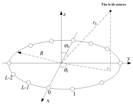
Figure 1.
The uniform circular array configuration.
We start with modeling the array received signal vector without unknown mutual coupling. Without loss of generality, all the sensors are located on the xy-plane and the UCA centre is set as the origin of the coordinate. At the same time, the FF source comes from (θk, φk) and the NF source comes from (θk,φk,rk), where θk∈[0,2π) denotes the azimuth angle measured counterclockwise from the x-axis and φk∈[0,π/2] denotes the elevation angle measured downward from the z-axis:
where, rk∈[0.62(D3/λ)1/2,2D2/λ) denotes the range of NF source, and rk∈[2D2/λ,∞) is the range of FF source, respectively. Therefore, rk∈[0.62(D3/λ)1/2,∞) denotes the range of mixed sources measured from the UCA center, where D = 2R represents the aperture of the array and λ symbolizes the incident sources wavelength. Consequently, the signal received by the l-th sensor can be modeled as:
where sk (t) is the k-th narrowband source, nl(t) is the additive Gaussian noise, and noises in different sensors are independent with the same variance σn2. Here, rl,k is the distance between the k-th source and the l-th sensor, which has the following form:
According to the Taylor series expansion, Formula (3) can be approximately given as follows
Consequently, Formula (1) can be expressed as
As a result, it is obvious that the FF source can be seen as a generalized NF source, the range parameter of which increases towards infinite.
According to the discussion in [5], the amplitude of mutual coupling coefficient (MCC) is in inverse proportion to the physical distance between each pair of sensors. In another word, the MCCs between neighboring sensors with a same adjacent space are almost equal to each other. Besides, the MCC would be approximately equal to zero when any two sensors are located enough far away. Consequently, we can model an L × L MCM of the UCA containing P + 1 (P ≤ M − 1) nonzero MCCs, and the symmetric Toeplitz matrix C is expressed as:
Therefore, the received signal vector under the unknown mutual coupling can be expressed in a matrix form:
where SN(t) and SF(t) denote the NF and FF signal vectors,
N(t) signifies L × 1 dimensional complex noise vector,
and AN and AF denote the steering vectors of NF source and FF source, respectively as
Throughout the paper, the following hypotheses are assumed to hold:
- The incoming source signals are statistically independent and zero-mean stationary random process;
- The sensor noise is the additive Gaussian one, which is independent from the source signals;
- The number of sources K1 and K2 are known as prior, and it satisfies K ≤ M.
3. Proposed Solution to Classification and Localization
In [27], the algorithm shows that the DOA estimation of FF sources is the precondition of MCM reconstruction. Therefore, improving the estimation accuracy of FF sources is helpful to improve the global estimation performance, including NF sources DOA and range estimations. In many practical applications, the algorithm must work against the situations of low signal noise ratio (SNR) and small number of snapshots. Fortunately, for a narrowband incoming source, we can use STP to improve the SNR of incoming sources based on its-self temporal coherence.
3.1. Space–Time Covariance Matrix
In practice, it is almost impossible to count an ideal covariance matrix. Hence, in algorithm execution process, covariance matrix must be estimated by a limited N snapshots sample, which is given as:
We assume that all the incoming signals are narrowband sources, therefore the following holds:
where m∈N, and z = exp(j2πfc/fs) is the time delay factor. Moreover, fs denotes the sampling pulse repetition frequency, and fc denotes the target carrier frequency. Here, we set Q time delay taps and only one sampling pulses between adjacent two time delay taps. The received data vector operated by STP can be written as:
where ⊗ is Kronecker product, IQ×Q denotes the Q × Q identity matrix and Z denotes the Q × 1matrix expressed as
According to the aforementioned assumptions, the received signal covariance matrix by STP can be calculated by:
where IQL×QL is the QL × QL identity matrix, and ∑N and ∑F are diagonal matrices,
3.2. FF Sources DOA and MCCs Estimation
By implementing eigenvalue decomposition (EVD) of RST, the following equation holds:
where, Λs is the diagonal matrix which contains the K largest eigenvalues. At the same time, Un is the QL × (QL − K) eigenvectors matrix which spans the noise subspace of RST, and Us is the QL × K signal eigenvectors matrix of RST which spans the signal subspace.
As the fact that the MCM is a column full rank Toeplitz matrix, the authors can construct a MUSIC spectrum search function to estimate DOAs and ranges parameters, which is expressed as:
From Formula (23), it is obvious that the computational cost of this equation is unbearable with the unknown C. Even if C is accurately estimated as a prior, it requires a 3D spectrum search to estimate and match the DOA and range parameters pair as well. In order to decrease the huge computational cost, the DOA estimation of FF sources must be decoupled from mixed sources estimates and MCM.
Referring to the discussion of mutual coupling problem with (ULA) in [5], Ca(θ, φ, r) in UCA could be reformulated as:
where c is the vector of P + 1 nonzero MCCs, which expressed as:
B(θ, φ, r) = B1 + B2 is composed of two L × (P + 1) matrices, and they are defined as:
where, {∙}p,q represents the element corresponding to the p-th row and q-th column of the matrix, [∙]p represents the element corresponding to p-th element of steering vector, and mod(p,q) denotes the modulus after dividing p by q.
It is obvious that Us and the combination of (IQ×Q⊗C)(Z⊗AN) and (IQ×Q⊗C)(Z⊗AF) can span the same signal subspace, and the signal subspace is orthogonal to the noise subspace spanned by Un. Therefore, the following equations hold:
Therefore, based on Formula (24)–(29), the FF sources’ DOAs can be estimated by the following spectrum search function:
where W(θ, φ) is defined as:
Note that c ≠ 0 and W(θ, φ) is a Hermite and nonnegative definite matrix. Based on the principle of RERA [29], cHW(θ, φ)c would be zero only when W(θ, φ) is a singular matrix. In other words, the determinant of W(θ, φ) would be equal to zero only when both parameters φ and θ are equal to any FF source’ DOA expressed by φk and θk (k = 1 + K1,…, K). Consequently, the FF sources’ DOAs could be estimated accurately by searching the K2 highest spectrum peaks through the following function:
where, det[∙] signifies the determinant of a matrix. From equation (32), it is easy seen that pF(θ, φ) is independently separated from equation (30). On the other hand, since the smallest eigenvalue of W(θ,φ) is also equal to zero when parameters φ and θ are equal to φk and θk (k = 1 + K1,…, K), the DOAs can also be estimated from the following spatial spectrum searching:
where, λmin[∙] denotes the smallest eigenvalue of a matrix. Therefore, the computational cost of estimating FF sources’ DOAs through (32) or (33) is effectively reduced compared with the multi-dimensional MUSIC spectrum search function. It is because of that, that only a 2D spectrum search process is required.
It is noteworthy that the proposed algorithm works in a similar way as that defined in [28,29]. However, the algorithm in [28] only solves the problem of pure FF signals, whereas the proposed algorithm aims to deal with the problem of mixed FF and NF signals. Moreover, the algorithm in [29] solves the mixed sources problem using a ULA. However, our work explicitly addresses the mixed sources problem under mutual coupling effect, using a UCA.
Substituting the estimated φk and θk (k = 1 + K1,…,K) and then perform eigendecomposition of W(θk,φk), we can obtain the smallest eigenvalue λmin and the corresponding eigenvector vmin, where vmin has been normalized by its first element. Finally, we can obtain the non-zero MCCs by:
According to the symmetric Toeplitz structure modeled as Formula (6), the MCM can be reconstructed after all MCCs have been calculated. Therefore, the reconstructed MCM could be used to eliminate the mutual coupling effects in the following signal processing process.
3.3. NF Sources DOA Estimation
This section begins with the discussion of MCM. It is noteworthy that the MCM of an UCA is different to that in an ULA, and it has some special properties based on its special array structure.
Remark 1:
The MCM C is a symmetric Toeplitz matrix, which holds:
and its inverse matrix is also a symmetric Toeplitz matrix, which holds:
Remark 2:
With C being a complex symmetric Toeplitz matrix, CCH is a real symmetric Toeplitz matrix (see Appendix A), which holds:
and the inverse matrix of CCH is also a real symmetric Toeplitz matrix, which holds:
As known, the estimation accuracy of NF sources will be improved as the SNR increases. If we can eliminate the noise, the SNR of NF will be approximately equal to infinity. Fortunately, the special properties of the MCM and array structure in UCA can be used to eliminate the noise and FF components effectively. Consequently, we can deal with the NF sources estimation problem only in a space domain with a high enough SNR.
According to Formula (17) and (19), the received signal covariance matrix only in space domain is expressed as:
After estimating and reconstructing mutual coupling matrix, the mutual coupling effects can be eliminated effectively. Therefore, we can get:
Based on the symmetric property of UCA configuration with an even number of sensors, the following holds:
Due to the fact that RF is a Hermitian matrix but RN only holds a Hermitian structure, we can obtain the following:
where J is the L × L particular transformational matrix which can be defined as:
where, IM×M denotes the M × M identity matrix. Consequently, the property differences between RF and RN can be utilized to implement the FF sources components elimination in the covariance matrix. Then, the differencing matrix can be expressed as:
where, AD is the virtual steering vectors expressed as:
Based on (13), (41) and (43), the following holds (see Appendix B)
where ⊙ denotes Hadamard product, and D is a rotation factor matrix defined as:
And then, by implementing the EVD of RD, the following holds:
where, Δs is a diagonal matrix which contains 2K1 non-zero eigenvalues, and γ0 is the zero eigenvalue, Vs is the L × 2K1 eigenvectors matrix spanning the signal subspace of RD, and Vn is the L × (L − 2K1) eigenvectors matrix spanning the noise subspace. It is obvious that the following holds:
Consequently, we can construct a diagonal matrix:
and the NF sources’ DOAs could be estimated accurately by searching the K1 highest spectrum peaks through the following function:
where Q denotes an arbitrary L × 2K1 full column rank matrix. The typical value of Q is set as that composed of arbitrary 2K1 columns of the L × L identity matrix. Conversely, since QH{JVs−Φ(θ,φ)Vs} contains zero eigenvalue only when φ and θ are equal to φk and θk (k = 1,…, K1), the DOAs can also be estimated from the following spatial spectrum searching:
In this subsection, the covariance differencing operation in UCA eliminate the FF components and noise effectively based on the structure differences between the NF and FF sources covariance matrices. As a conclusion, the proposed algorithm successfully avoids the 3D spectrum searching and sources classification processing with the help of covariance differencing.
3.4. NF Sources Range Estimation
After estimating the NF sources’ DOAs and replacing the unknown DOA variable pairs in the following equation by the estimated ones, the k-th NF source’ range parameter can be estimated by:
From the above equation, it shows that the estimation results of both DOA and range parameters would be paired together automatically without any parameters matching processing.
3.5. The Proposed Algorithm Summary
In order to show the specific execution process, the proposed algorithm can be summarized as following.
- STEP 1.
- Estimate the STP covariance matrix through Formula (19).
- STEP 2.
- Eigen decompose the STP covariance matrix to generate its noise subspace.
- STEP 3.
- Estimate the FF sources’ DOAs through the RERA estimator by Formula (32) or (33).
- STEP 4.
- Obtain the MCCs by Formula (34), and construct the MCM by Formula (6).
- STEP 5.
- Compensate the MCM and by Formula (40).
- STEP 6.
- Construct the differencing matrix by Formula (45).
- STEP 7.
- Eigen decompose the differencing matrix to generate its noise subspace.
- STEP 8.
- Estimate the DOAs of NF sources through Formula (52) or (53).
- STEP 9.
- Estimate the range parameter of NF sources through Formula (54).
4. Discussion
4.1. Number of Required Array Elements
In order to get the unique solution of (32) or (33), W(θ,φ) must be invertible at non-incident direction. Due to the fact that all the incident sources have the same carrier frequency, the extended freedom degree by time delay is invalid. Furthermore, the maximum rank of Z⊗B(θ, φ, ∞) maybe M, and the space domain freedom degree of UnUnH is L−K, they must satisfy:
consequently, the parameter identifiability condition of the algorithm is K ≤ M.
Moreover, in order to estimate the MCCs, [W(θ,φ)] must be equal to zero at least once. In the other word, at least one FF source is required to be used for MCCs estimation.
4.2. Contribution of STP
By eigenvalue decomposition, the covariance matrix RST can be decomposed as shown in (22), here Λs is the diagonal matrix which contains the K largest eigenvalues:
and the eigenvalues hold the following comparison expression:
In fact, eigenvalue composition is the unitized orthogonalization processing of steering vectors. Therefore, each eigenvalue is a linear combination of all signals and noise power, and the i-th eigenvalue can be expressed as:
where αi,k∈(0,1) is the power factor whose value depends on the projection of steering vectors and relative power ratios of all sources, and sk2 denotes the power of the k-th source. Compared with pure space domain processing, the eigenvalues are almost enlarged Q times. Thus, we define the power gain by STP as:
Consequently, it is equivalent to improving the SNR of incoming signals.
4.3. Computational Complexity
In order to compare computational complexity intuitively, TSMUSIC-like and CD-like and algorithms are set as comparison objects of the proposed algorithm. For all three algorithms, the major computation processes are calculating statistical matrices, eigenvalue decomposing and spectrum searching. It is defined that the search step of azimuth θ∈(0°,360°] is θΔ, the search step of elevation φ ∈(0°,90°] is φΔ, and the search step of r∈[0.62(D3/λ)1/2,2D2/λ] is rΔ for K1 NF sources. We assume that N is the number of snapshots.
For TSMUSIC-like algorithm, the major computations are to compute an L × L FOC matrix and an L × L second-order cumulant one, and to implement the EVDs of the two matrices for spatial searching twice. For CD-like algorithm the major computations are to form an L × L covariance matrix and an L × L noise subspace matrix, and to implement once EVD of the covariance matrix. After that, three times spatial searching are required to estimate the NF sources’ DOAs, the ranges of NF sources and the FF sources’ DOAs. The proposed algorithm constructs a second-order cumulant space–time matrix. The major computations are to implement the EVDs of the QL × QL covariance matrix and the L × L differencing matrix, and to perform three times spatial search for estimating DOA and range. Consequently, the computational complexity of the three algorithms is shown in Table 1.

Table 1.
Computational complexity comparison.
However, in order to ensure sufficient measuring precision, the search steps are usually set as very small values. Therefore, the computational burden of spectral search is huge, which is usually more than 90 percent of the total computational cost. In this case, the computational cost of proposed algorithm is approximately equal to that of CD-like, and almost twice as that of TSMUSIC-like.
4.4. Capacity for Mixed Sources Classification
From the above analysis, it is obvious that TSMUSIC-like algorithm cannot classify the mixed sources autonomously. Especially if the FF sources and the NF sources have the same DOA, the TSMUSIC-like algorithm would be invalid. Fortunately, the CD-like algorithm and proposed algorithm can eliminate FF component when estimating the NF sources. However, the CD-like algorithm ignores the mutual coupling effect.
4.5. DOA Ambiguity
In order to avoid DOA ambiguity in UCA, we must construct Φ(θ,φ) without ambiguity, i.e., the steering vector d(θ,φ) must be unique at different incident-directions. Therefore, the aperture of UCA dealing with mixed sources problem must be set as a half of that, solving pure FF sources estimation without ambiguity. For the similar question in ULA, the inter-space is usually set as a quarter of wavelength, half of the normal inter-space.
5. Simulation Results
Some simulations are conducted in this section to evaluate the proposed algorithm. A UCA of 10 elements with radius R = λ is taken into consideration. The input signal to noise ratio (SNR) of the k-th source is defined as 10 × log10(σk2/σn2), where σk2 denotes the power of the k-th source, and σn2 denotes the noise power. We assume that all the sources are with equal power. In the following experiments, the performance is measured by the root mean square error (RMSE) of 200 independent Monte Carlo experiments. It is noted that the estimation performance of the range parameters is only for the NF sources experiment. Hence, we do not give the estimation performance of the range parameters of FF sources.
5.1. Spectrums of DOA and Range Estimation
In the first simulation, the authors consider a scenario in where two NF sources and two FF sources coexist, and they are located at {θ1 = 43°, φ1 = 65°, r1 = 1.7λ}, {θ2 = 137°, φ2 = 65°, r2 = 2.6λ}, {θ3 = 197°, φ3 = 65°, r3 = ∞} and {θ4 = 261°, φ4 = 65°, r4 = ∞}. In order to show the intuitive comparison of different spatial spectrums, we set all sources with the same elevation. The number of snapshots is set as 400 and the SNR of all sources is set as 5 dB. And, the nonzero MCCs are set as [1, −0.0492 + 0.0129i, 0.0018 − 0.0098i]. The DOA and range spectrums of the three algorithms are shown in the following figures.
From Figure 2a, it shows that TSMUSIC-like generates four highest sharp spectrum peaks on the directions of NF and FF sources. However, there are other false peaks caused by the unknown mutual coupling, which would lead to false estimation. Compared with the DOA spectrum after MCM elimination, it obviously shows that this algorithm generates serious error in DOA estimation. Assuming that NF and FF sources have been classified, the range spectrum of NF sources by TSMUSIC-like is shown in Figure 2b. Similarly, this algorithm generates unreliable results in range estimation, without MCM elimination.
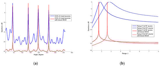
Figure 2.
(a) Azimuth spectrum of two stage multiple signal classification (TSMUSIC)-like at φ = 65°; (b) Range spectrum of TSMUSIC-like.
In Figure 3a, it shows that CD-like generates worse spectrums of NF and FF sources than that in Figure 2a. This is because that the structural properties of array steering vectors are invalid under unknown mutual coupling. In particular, there may be fatal errors in DOA estimation of NF sources, as shown in detail. In Figure 3b, due to the propagation error and model mismatching, this algorithm generates serious error in range estimation without MCM elimination.
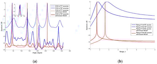
Figure 3.
(a) Azimuth spectrum of covariance differencing (CD)-like at φ = 65°; (b) Range spectrum of CD-like.
In Figure 4a, it shows that the proposed algorithm generates two sharp peaks in spectrum of NF sources and another two sharp peaks in that of FF sources, corresponding to the actual DOAs of mixed sources. The range estimation is shown in Figure 4b, it shows that the proposed algorithm can generate reliable range estimation results as well.
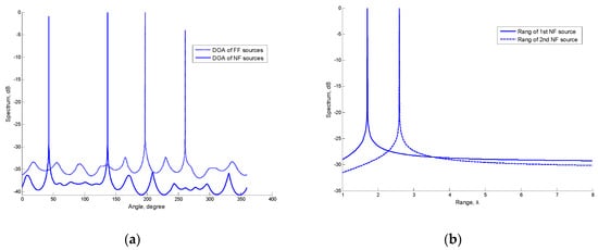
Figure 4.
(a) Azimuth spectrum of proposed at φ = 65°; (b) Range spectrum of proposed.
5.2. Performance versus Snapshot Number
In the second simulation, the authors consider a scenario in where one NF source and one FF sources coexist, and the location parameters are {θ5 = 77°, φ5 = 47°, r5 = 2.2λ} and {θ6 = 259°, φ6 = 58°, r6 = ∞}, with the SNR being set as 10 dB. And the time delay tap number of the proposed algorithm is set as Q = 3. The nonzero MCCs are set as the same as those in the first experiment and the number of snapshots varies from 100 to 1000.
The RMSEs of the DOA and range estimates, as the snapshot number changes, are shown in Figure 5 and Figure 6. It obviously shows that both the DOA and the range estimation RMSEs of the proposed algorithm decrease monotonically as the snapshot number increases. It is due to the fact that a larger sampling number will produce better estimate of the covariance matrix for stationary data. Compared with the proposed algorithm, the DOA RMSEs of the other two algorithms no longer decrease as the number of snapshots increases, shown in Figure 5a. It is because that steering mismatching caused by mutual coupling effect. Moreover, as shown in Figure 5b, TSMUSIC-like estimates the DOAs of mixed sources in the same search, hence the mixed sources have the similar RMSEs with known MCM. On the other hand, CD-like performances better results of NF sources than that of FF sources, due to the covariance differencing operation with known MCM. As known, in proposed algorithm, FF source DOA estimation is the precondition of NF source DOA estimation, hence the propagation error will degrade NF DOA estimation. In addition, the proposed algorithm produces the best performance because of STP. A similar result is also obtained in range estimation as shown in Figure 6.
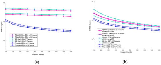
Figure 5.
(a) Root mean square error (RMSEs) of the direction of arrival (DOA) estimates versus snapshot number; (b) RMSEs of the DOA estimates versus snapshot number with known mutual coupling matrix (MCM).
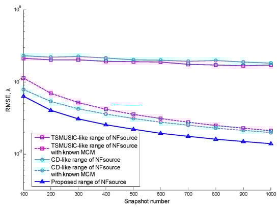
Figure 6.
RMSEs of the range estimates versus snapshot number.
5.3. Performance versus SNR
In the third simulation, almost all simulation conditions are adopted as the same as those in the second experiment, except that the number of snapshots is set as 400, and the SNR varies from −5 dB to 20 dB.
The RMSEs of the DOA and range estimates, as the changes of SNR, are shown from Figure 7 and Figure 8. Compared with the proposed algorithm, both the DOA and range RMSEs of the other two algorithms no longer decrease as the SNR increases due to mutual coupling effect. It shows that only the proposed algorithm can provide satisfactory DOA estimation performance of mixed sources in Figure 7a. Moreover, in Figure 7b, FF source DOA RMSEs by TSMUSIC-like are similar to NF ones by itself with known MCM. Respectively, CD-like produces better results of NF sources and worse results of FF sources than those by TSMUSIC-like. Additionally, in the proposed algorithm, the propagation error will degrade NF DOA estimation. As a result, the proposed algorithm outperforms the other two algorithms in both DOA and range estimation shown in Figure 8, because of STP.
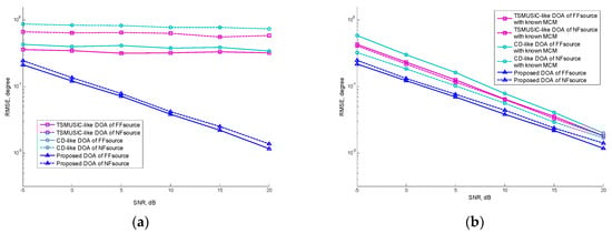
Figure 7.
(a) RMSEs of the DOA estimates versus signal noise ratio (SNR); (b) RMSEs of the DOA estimates versus SNR with known MCM.
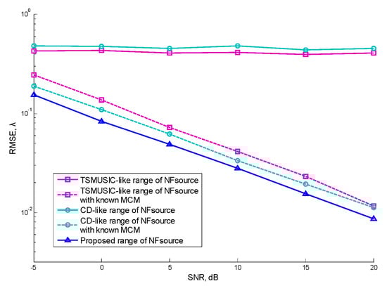
Figure 8.
RMSEs of the range estimates versus SNR.
6. Conclusions
In this paper, a high performance joint space–time classification and localization algorithm for mixed sources in the presence of unknown mutual coupling in UCA is proposed. Compared with the aforementioned algorithms, the proposed algorithm is effective in mixed sources classification and localization, and it can provide a better DOA and range estimation performance under the mutual coupling effect. In addition, for computational complexity, the proposed algorithm successfully avoids multi-dimensional spectrum search (including MCCs and range), parameter matching and high-order cumulant. Finally, many simulation results give forceful proof that the proposed algorithm is efficient for mixed sources classification and localization under unknown mutual coupling in UCA, especially in the case of low SNR and small snapshot number.
Author Contributions
Conceptualization, L.W. and Y.W.; Methodology, K.W. and J.X.; Writing—original draft preparation, K.W.; Writing—review and editing, Y.W.; Supervision, Z.Z.
Funding
This work is supported by the National Natural Science Foundation of China under Grant No. 61771404, No. 61601372 and No. 61801390. It is also funded by the Science, Technology and Innovation Commission of Shenzhen Municipality under Grant No. JCY20170306154016149, JCY20170815154325384.
Conflicts of Interest
The authors declare no conflict of interest.
Appendix A
Without loss of generality, we replace the zero coefficients with unknown complex ones, and C is an L × L symmetric Toeplitz matrix. We defined that:
When L is odd, i.e., L = 2P + 1, the MCM is constructed as:
it is clear that the elements in RC are expressed as:
and it clearly shows that there are P pairs of conjugate coefficients and a real one in each element, and the elements on each minor diagonal are same.
When L is even, i.e., L = 2P, the MCM is constructed as:
Therefore, the elements in RC are expressed as:
It noticeably shows that there are P pairs of conjugate coefficients in each element, and the elements on each minor diagonal are same. Consequently, RC is real symmetric Toeplitz matrix.
Appendix B
According to (41), the virtual steering vectors AD is expressed as:
It is clear that the followings holds:
therefore, AD satisfies:
References
- Roy, R.; Kailath, T. ESPRIT-estimation of signal parameters via rotational invariance techniques. IEEE Trans. Acoust. Speech Signal Process. 1989, 37, 984–995. [Google Scholar] [CrossRef]
- Cao, M.Y.; Huang, L.; Qian, C.; Xue, J.Y.; So, H.C. Underdetermined DOA estimation of quasi-stationary signals via Khatri–Rao structure for uniform circular array. Signal Process. 2015, 106, 41–48. [Google Scholar] [CrossRef]
- Schmidt, R. Multiple emitter location and signal parameter estimation. IEEE Trans. Antennas Propag. 1986, 34, 276–280. [Google Scholar] [CrossRef]
- Qian, C.; Huang, L.; SO, H.C. Computationally efficient ESPRIT algorithm for direction-of-arrival estimation based on Nyström method. Signal Process. 2014, 94, 74–80. [Google Scholar] [CrossRef]
- Wang, Y.; Trinkle, M.; NG, B.W.-H. DOA estimation under unknown mutual coupling and multipath with improved effective array aperture. Sensors 2015, 15, 30856–30869. [Google Scholar] [CrossRef]
- Huang, Y.; Barkat, M. Near-field multiple source localization by passive sensor array. IEEE Trans. Antennas Propag. 1991, 39, 968–975. [Google Scholar] [CrossRef]
- Zhi, W.; Chia, M.Y.W. Near-field source localization via symmetric subarrays. IEEE Signal Process. Lett. 2007, 14, 409–412. [Google Scholar] [CrossRef]
- He, J.; Ahmad, M.O.; Swamy, M. Near-field localization of partially polarized sources with a cross-dipole array. IEEE Trans. Aerosp. Electron. Syst. 2013, 49, 857–870. [Google Scholar] [CrossRef]
- Tao, J.; Liu, L.; Lin, Z. Joint DOA, range, and polarization estimation in the Fresnel region. IEEE Trans. Aerosp. Electron. Syst. 2011, 47, 2657–2672. [Google Scholar] [CrossRef]
- Xie, J.; Tao, H.; Rao, X.; Su, J. Efficient method of passive localization for near-field noncircular sources. IEEE Antennas Wirel. Propag. Lett. 2015, 14, 1223–1226. [Google Scholar] [CrossRef]
- Xie, J.; Tao, H.; Rao, X.; Su, J. Real-valued localisation algorithm for near-field non-circular sources. Electron. Lett. 2015, 51, 1330–1331. [Google Scholar] [CrossRef]
- Lee, J.; Chen, Y.; Yeh, C. Covariance approximation method for near-field direction-finding using a uniform linear array. IEEE Trans. Signal Process. 1995, 43, 1293–1298. [Google Scholar]
- Noh, H.; Lee, C.A. covariance approximation method for near-field coherent sources localization using uniform linear array. IEEE J. Ocean. Eng. 2015, 40, 187–195. [Google Scholar] [CrossRef]
- Grosicki, E.; Abed-Meraim, K.; Hua, Y. A weighted linear prediction method for near-field source localization. IEEE Trans. Signal Process. 2005, 53, 3651–3660. [Google Scholar] [CrossRef]
- Liang, J.; Liu, D. Passive localization of near-field sources using cumulant. IEEE Sens. J. 2009, 9, 953–960. [Google Scholar] [CrossRef]
- Liang, J.; Liu, D. Passive localization of mixed near-field and far-field sources using two-stage MUSIC algorithm. IEEE Trans. Signal Process. 2010, 58, 108–120. [Google Scholar] [CrossRef]
- He, J.; Swamy, M.N.S.; Ahmad, M.O. Efficient application of MUSIC algorithm under the coexistence of far-field and near-field sources. IEEE Trans. Signal Process. 2012, 60, 2066–2070. [Google Scholar] [CrossRef]
- Wang, B.; Liu, J.; Sun, X. Mixed sources localization based on sparse signal reconstruction. IEEE Signal Process. Lett. 2012, 19, 487–490. [Google Scholar] [CrossRef]
- Wang, B.; Zhao, Y.; Liu, J. Mixed-order MUSIC algorithm for localization of far-field and near-field sources. IEEE Signal Process. Lett. 2013, 20, 311–314. [Google Scholar] [CrossRef]
- Liu, G.; Sun, X. Two-stage matrix differencing algorithm for mixed far-field and near-field sources classification and localization. IEEE Sens. J. 2014, 14, 1957–1965. [Google Scholar]
- Liu, G.; Sun, X.; Liu, Y.; Qin, Y. Low-complexity estimation of signal parameters via rotational invariance techniques algorithm for mixed far-field and near-field cyclostationary sources localization. IET Signal Process. 2013, 7, 382–388. [Google Scholar] [CrossRef]
- Jiang, J.; Duan, F.; Chen, J.; Li, Y.; Hua, X. Mixed near-field and far-field sources localization using the uniform linear sensor array. IEEE Sens. J. 2013, 13, 3136–3143. [Google Scholar] [CrossRef]
- Ye, Z.; Dai, J.; Xu, X.; Wu, X. DOA estimation for uniform linear array with mutual coupling. IEEE Trans. Aerosp. Electron. Syst. 2009, 45, 280–288. [Google Scholar]
- Xu, X.; Ye, Z.; Zhang, Y. DOA estimation for mixed signals in the presence of mutual coupling. IEEE Trans. Signal Process. 2009, 57, 3523–3532. [Google Scholar] [CrossRef]
- Liu, C.; Ye, Z.; Zhang, Y. DOA estimation based on fourth-order cumulants with unknown mutual coupling. Signal Process. 2009, 89, 1819–1843. [Google Scholar] [CrossRef]
- Liao, B.; Zhang, Z.G.; Chan, S.C. DOA estimation and tracking of ULAs with mutual coupling. IEEE Trans. Aerosp. Electron. Syst. 2012, 48, 891–905. [Google Scholar] [CrossRef]
- Xie, J.; Tao, H.; Rao, X.; Su, J. Localization of mixed far-field and near-field sources under unknown mutual coupling. IEEE Trans. Signal Process. 2016, 50, 229–239. [Google Scholar] [CrossRef]
- Wu, Y.; So, H.C. Simple and accurate two dimensional angle estimation for a single source with uniform circular array. IEEE Antennas Wirel. Propag. Lett. 2008, 7, 78–80. [Google Scholar]
- Goossens, R.; Rogier, H. A hybrid UCA-RARE/Root-MUSIC approach for 2-D direction of arrival estimation in uniform circular arrays in the presence of mutual coupling. IEEE Trans. Antennas Propag. 2007, 55, 841–849. [Google Scholar] [CrossRef]
- Qi, C.; Wang, Y.; Zhang, Y.; Chen, H. DOA estimation and self-calibration algorithm for uniform circular array. Electron. Lett. 2009, 41, 1092–1094. [Google Scholar] [CrossRef]
- Lin, M.; Yang, L. Blind calibration and DOA estimation with uniform circular arrays in the presence of mutual coupling. IEEE Antennas Wirel. Propag. Lett. 2006, 5, 315–318. [Google Scholar] [CrossRef]
- Xiang, L.; Ye, Z.; Xu, X.; Chang, C.; Xu, W.; Hung, Y.S. Direction of arrival estimation for uniform circular array based on fourth-order cumulants in the presence of unknown mutual coupling. IET Microw. Antennas Propag. 2008, 2, 281–287. [Google Scholar] [CrossRef]
- Wu, Y.; Wang, H.; Zhang, Y.; Wang, Y. Multiple near-field source localisation with uniform circular array. Electron. Lett. 2013, 49, 1509–1510. [Google Scholar] [CrossRef]
- Xue, B.; Fang, G.; Ji, Y. Passive localisation of mixed far-field and near-field sources using uniform circular array. Electron. Lett. 2016, 52, 1690–1692. [Google Scholar] [CrossRef]
- Cristallini, D.; Burger, W. A Robust Direct Data Domain Approach for STAP. IEEE Trans. Signal Process. 2012, 60, 1283–1294. [Google Scholar] [CrossRef]
- Ahmadi, M.; Mohamed-pour, K. Robust space-time adaptive processing against Doppler and direction-of-arrival mismatches. In Proceedings of the Microwaves, Radar and Remote Sensing Symposium, Kiev, Ukraine, 25–27 August 2011; pp. 305–308. [Google Scholar]
© 2019 by the authors. Licensee MDPI, Basel, Switzerland. This article is an open access article distributed under the terms and conditions of the Creative Commons Attribution (CC BY) license (http://creativecommons.org/licenses/by/4.0/).